The Mixmaster Universe is Unambiguously Chaotic

The Mixmaster or Bianchi IX cosmological model has become one of the archetypal settings for studying gravitational dynamics. The past decade has seen a vigourous debate about whether or not the Mixmaster’s dynamics is chaotic. In this talk we review our recent work in uncovering a chaotic invariant set of orbits in the Mixmaster phase space, and how we used this discovery to prove the dynamics is chaotic.

1 The mixmaster universe

The mixmaster model$\!{}^{{\bf?},{\bf?}}$ describes a homogeneous but anisotropic closed cosmology of Bianchi type IX. The spatial sections have the geometry of a deformed three-sphere, evolving with three independent scale factors, $a(t),b(t),c(t)$. The vacuum field equations read:

$$(\ln a^{2})^{\prime\prime}=(b^{2}-c^{2})^{2}-a^{4}\quad{\it et\;cyc.\;}(a,b,c)\,.$$ (1)

Here a prime denotes $d/d\tau$ and $dt=abc\;d\tau$. When the right hand sides of the three equations (1) are all $\approx 0$, ie. when the minisuperspace potential

$$V=a^{4}+b^{4}+c^{4}-2(a^{2}b^{2}+a^{2}c^{2}+b^{2}c^{2})\approx 0\,,$$ (2)

the universe evolves in an approximate Kasner phase with $a\sim t^{p_{i}},\;b\sim t^{p_{j}},\;c\sim t^{p_{k}}$. The Kasner exponents satisfy $\sum_{i=1}^{3}p_{i}=\sum_{i=1}^{3}p_{i}^{2}=1$.

The dynamics of the model can be separated into the evolution of an overall scale factor $\Omega$, and two variables that measure the departure from isotropy$\!{}^{{\bf?}}$:

$$\Omega=\frac{1}{3}\ln(abc),\quad\beta_{+}=\frac{1}{3}\ln(bc/a^{2}),\quad\beta_{-}=\frac{1}{\sqrt{3}}\ln(b/c)\,.$$ (3)

Since it can be shown$\!{}^{{\bf?}}$ that the evolution of $\Omega$ describes a smooth overall expansion and contraction of the universe, any chaotic behaviour must be associated with motion in the anisotropy plane $(\beta_{+},\beta_{-})$.

Early work on the mixmaster dynamics focused on discrete maps$\!{}^{{\bf?}}$ that were used to approximate the continuum dynamics. The maps were shown to be chaotic$\!{}^{{\bf?},{\bf?}}$, and from this it was inferred that the full dynamics was also chaotic. The picture became clouded in the late eighties when numerical studies of the dynamics found that the principle Lyapunov exponent vanished$\!{}^{{\bf?}}$, indicating that the system was not chaotic. Subsequently, two possible causes for the discrepancy were isolated$\!{}^{{\bf?}}$: (1) the full dynamics might be integrable, but the approximate maps fail to preserve all the constants of motion; (2) the full dynamics is chaotic but the Lyapunov exponents vanish for certain choices of time coordinate. The second possibility raised the important issue of how to describe chaos in a coordinate invariant way. We address this question in our other contribution to this volume. In the remainder of this talk we describe how coordinate independent methods can be used to settle the mixmaster debate in favour of option (2). That is, the mixmaster universe is chaotic and the approximate maps do capture the essential features of the dynamics.

2 Uncovering the chaotic invariant set

The key to understanding the mixmaster dynamics can be found in the very first papers on the subject$\!{}^{{\bf?},{\bf?}}$. These papers identify three “attractors” for the dynamics corresponding to the three states of highly anisotropic expansion $a\sim b\sim{\rm const.},\;c\sim t$, $c\sim a\sim{\rm const.},\;b\sim t$ and $b\sim c\sim{\rm const.},\;a\sim t$. The $SO(3)$ symmetry of the spatial sections ensures that all three possibilities occur with equal probability. If these attractors corresponded to final outcomes, it would be a simple matter to decide if the dynamics was chaotic. All one would have to do is assign a colour to each outcome, then colour-code the space of initial conditions according to the outcomes. If the boundaries between the three outcomes are fractal, then the dynamics is chaotic.

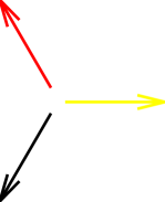
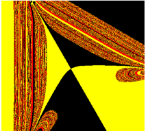
Figure 1: (i) The minisuperspace potential with exits cut in the corners and outcomes marked by arrows. (ii) Outcome basins and their fractal boundaries in the anisotropy plane.

Unfortunately, the procedure is not so simple as the attractors do not correspond to final outcomes. When viewed in the anisotropy plane, the attractors correspond to trajectories that go deep into one of the three corners of the minisuperspace potential (see Fig.(1.i)). After a long time, the trajectory returns to the scattering region close to the centre of the triangular potential before again scattering toward one of the three attractors.

We reasoned that if the mixmaster was chaotic, it must correspond to a non-compact billiard$\!{}^{{\bf?}}$. Moreover, there should be a chaotic invariant set of unstable periodic orbits in the centre of the scattering region. In order to uncover this set we set a threshold based on the relative rate of expansion of the three scale factors. When one axis was collapsing very much faster than the other two we stopped the evolution and assigned an outcome. This is equivalent to cutting pockets in the corners of the minisuperspace potential, as shown in Fig.(1.i). In effect we simplified the analysis by converting the mixmaster into a Hamiltonian exit system$\!{}^{{\bf?}}$. We can do this with confidence since a system with exits is always less chaotic than the corresponding system without exits.

With exits in place it is a simple matter to numerically plot the attractor basin boundaries. A representative slice through phase space is shown in Fig.(1.ii). The basin boundaries are clearly fractal, and were found to have an information dimension$\!{}^{{\bf?}}$ of $D_{1}=1.86\pm 0.02$. From this we can conclude in a coordinate independent way that the mixmaster universe is chaotic. Moreover, exactly the same procedure can be used to show that the Bianchi VIII cosmological model is chaotic.

Trajectories belonging to the boundaries of the attractor basins are future asymptotic to the unstable periodic orbits that comprise the mixmaster’s chaotic invariant set. (There are actually no truly periodic orbits in the $(\beta_{+},\beta_{-})$ plane since the overall anisotropy increases as a cosmological singularity is approached. The orbits are self-similar rather than periodic. However, rescaled coordinates can be found where the orbits are periodic). The complexity of the mixmaster system can be measured by introducing a symbolic coding for the periodic orbits. (A similar coding was introduced by Rugh$\!{}^{{\bf?}}$ for the aperiodic orbits). The most efficient way of coding an orbit is shown in Fig.(1.i). The symbol x, y, or z is recorded each time the trajectory passes through one of the three triangular regions bounded by the corners of the potential. The simplest periodic orbit, first found by Misner$\!{}^{{\bf?}}$, corresponds to the repeated sequence ${\bf xyz}$. All the periodic orbits can be similarly described, and it is easy to show that the number of orbits made from words of length $k$ grows as $N(k)\sim 2^{k}$. Since the number of orbits grows exponentially with length, the collection of periodic orbits has a non-zero topological entropy, in this case, $H_{T}=\ln 2$, which implies the dynamics is chaotic.

References

References

- [1] C. W. Misner, Phys. Rev. Lett. 22, 1071, (1969).
- [2] I. M. Khalatnikov & E. M. Lifshitz, Phys. Rev. Lett. 24, 76 (1970); V. A. Belinskii, I. M. Khalatnikov & E. M. Lifshitz, Adv. Phys. 19, 525 (1970); ibid 31, 639 (1982).
- [3] X. Lin & R. M. Wald, Phys. Rev. D41 2444 (1990).
- [4] J. D. Barrow, Phys. Rev. Lett. 46, 963 (1981); Phys. Rep. 85, 1 (1982).
- [5] G. Francisco & G. E. A. Matsas, Gen. Rel. Grav. 20, 1047 (1988).
- [6] Deterministic chaos in general relativity eds. D. Hobill, A. Burd & A. Coley, (Plenum Press, New York, 1994).
- [7] N. J. Cornish & J. J. Levin, Phys. Rev. Lett. 78, 998 (1997); Phys. Rev. D55 7489 (1997).
- [8] S. Bleher, C. Grebogi, E. Ott & R. Brown, Phys. Rev. A38, 930 (1988).