The extent of computation in Malament-Hogarth spacetimes

Abstract

We analyse the extent of possible computations following Hogarth [7] in Malament-Hogarth (MH) spacetimes, and Etesi and Németi [3] in the special subclass containing rotating Kerr black holes.  [7] had shown that any arithmetic statement could be resolved in a suitable MH spacetime. [3] had shown that some $\forall\exists$ relations on natural numbers which are neither universal nor co-universal, can be decided in Kerr spacetimes, and had asked specifically as to the extent of computational limits there. The purpose of this note is to address this question, and further show that MH spacetimes can compute far beyond the arithmetic: effectively Borel statements (so hyperarithmetic in second order number theory, or the structure of analysis) can likewise be resolved:

Theorem A. If $H$ is any hyperarithmetic predicate on integers, then there is an MH spacetime in which any query $?n\in H?$ can be computed.

In one sense this is best possible, as there is an upper bound to computational ability in any spacetime which is thus a universal constant of the space-time $\mathcal{M}$.

Theorem C. Assuming the (modest and standard) requirement that space-time manifolds be paracompact and Hausdorff, for any MH spacetime $\mathcal{M}$ there will be a countable ordinal upper bound, $w(\text{$\mathcal{M}$)}$, on the complexity of questions in the Borel hierarchy resolvable in it.

1 Introduction

Hogarth has shown that not only any universal statement, such as Goldbach’s Conjecture, but any arithmetical statement can be resolved in finite time, in a suitable Malament-Hogarth (MH) space-time (these are defined in 1.1 below).

Our main observations are twofold: firstly that there is no reason for Hogarth to stop at first order statements of arithmetic: effectively Borel statements (so hyperarithmetic in second order number theory, or the structure of analysis) can likewise be resolved (Section 2):

Theorem A. If $H$ is any hyperarithmetic predicate on integers, then there is an MH in which any query $?n\in H?$ can be computed.

In fact for any transfinite Borel statement about the integers one can define a MH spacetime in which the statement can be resolved.

In one sense this is best possible, as secondly, there is an upper bound to computational ability in any spacetime, which is thus a universal constant of the space-time $\mathcal{M}$ (Section 3). The following is merely an observation:

Theorem C. Assuming the (modest and standard) requirement that space-time manifolds be paracompact and Hausdorff, for any MH spacetime $\mathcal{M}$ there will be a countable ordinal upper bound, $w(\text{$\mathcal{M}$)}$, on the complexity of predicates in the Borel hierarchy resolvable in it.

Etesi and Németi noted in [3] that some $\forall\exists$ relations on natural numbers which are neither universal $(\forall)$ nor co-universal $(\exists)$, can be decided in certain MH spacetimes (instantiated by rotating Kerr black holes) and they ask specifically as to the extent of computational limits in such spacetimes.

Theorem B. The relations $R\subseteq\mathbbm{N}$ computable in the spacetimes of [3] form a subclass of the $\Delta_{2}$-relations on $\mathbbm{N}$; this is a proper subclass if and only if there is a fixed finite bound on the number of signals sent to the observer on the finite length path.

This is treated in Sect 2.2.

1.1 History and preliminaries

Pitowsky [9] gives an account of an attempt to define spacetimes in which supertasks can almost be completed - essentially they allow the result of infinitely many computations by one observer $O_{r}$ (he used the, as then unsolved, example of Fermat’s Last Theorem) performed on their infinite (i.e. endless in proper time) world line $\gamma_{1}$, to check whether there exists a triple of integers $x^{k}+y^{k}=z^{k}$ for some $k>2$ as a counterexample to the Theorem or not. If a counterexample was found a signal would be sent to another observer $O_{p}$ travelling along a world line $\gamma_{2}$. The difference being that the proper time along $\gamma_{2}$ was finite, and thus $O_{p}$ could know the truth or falsity of the Theorem in a (for them) finite time, depending on whether a signal was received or not. As Earman and Norton [1] mention, there are problems with this account not least that along $\gamma_{2}$ $O_{p}$ must undergo unbounded acceleration.

Malament and Hogarth alighted upon a different spacetime example. The following definition comes from [1]:

Definition 1

$\text{$\mathcal{M}$=}(M,g_{\operatorname{ab}})$ is a Malament-Hogarth (MH) spacetime just in case there is a time-like half-curve $\gamma_{1}\subset M$ and a point $p\in M$ such that $\int_{\gamma_{1}}d\tau=\infty$ and $\gamma_{1}\subset I^{-}(p)$.

(Here $\tau$ is proper time.) As they remark this makes no reference to the word-line of a receiver of messages $O_{p}$ travelling along a $\gamma_{2}$, but point out that there will be in any case such a future-directed timelike curve $\gamma_{2}$ from a point $q\in I^{-}(p)$ to $p$ such that $\int_{\gamma_{2}(q,p)}d\tau<\infty$, with $q$ chosen to lie in the causal future of the past endpoint of $\gamma_{2}$.  As Hogarth showed in [6] such spacetimes are not globally hyperbolic, thus ruling out many “standard” space-times (such as Minkowski space-time). Earman and Norton’s diagram of a “toy MH space-time” is Figure 1.1 below. Hogarth’s perhaps more succinct picture is on the right.

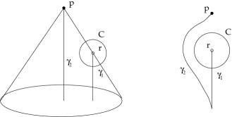
Figure 1:

To rerun (and update) the Pitowski argument: the proper time along $\gamma_{1}$ is infinite, thus a Turing machine can be programmed to look for counterexamples to the Goldbach Conjecture (or any other proposition involving a single universal quantifier over an unquantified matrix: $\forall nP(n)$) by checking $P(0),P(1),\ldots$ each of which in turn only takes a finite amount of time; if a counterexample is found a signal is sent out to the observer $\mathcal{O}_{p}$ travelling along the finite proper time curve $\gamma_{2}$. If no signal is received by the time $\mathcal{O}_{p}$ reaches $p$ then $\mathcal{O}_{p}$ knows that the Conjecture is true. Either way $\mathcal{O}_{p}$ is supposed to have discovered the truth by this point.

To obtain a spacetime as above, they take Minkowski spacetime $\mathcal{N}_{0}=(\mathbbm{R}^{4},\eta_{\operatorname{ab}})$ and choose a scalar field $\Omega$ which is everywhere equal to 1 outside of a compact set $C$, and which rapidly goes to $+\infty$ as the point $r$ is approached. The point $r$ is removed and the MH spacetime is then $\mathcal{N}=(\mathbbm{R}^{4}\backslash\{r\},g_{\operatorname{ab}})$, where $g_{\operatorname{ab}}=\Omega^{2}\eta_{\operatorname{ab}}$. $\Omega$ and $\gamma_{1}$ can be chosen so that $\gamma_{1}$ is a timelike geodesic.

Earman and Norton discuss at length the physical possibilities and difficulties of this scenario: Gödel spacetimes are MH, but are causally vicious; the toy spacetime above need not satisfy any energy conditions; anti-de Sitter spacetime is MH, but fails a strong energy condition; Reissner-Nordstrom spacetime meets this, but as in all MH spacetimes there is divergent blue-shift of the signal to $\mathcal{O}_{p}$; further, of the unbounded amplification of signals that $\mathcal{O}_{p}$ may have to receive, etc., etc.  It is not our aim here to add to this discussion on physical viabilities but to make some observations on the purely logico-mathematical possibilities and boundaries of this kind of arrangement.

Logicians accordingly calibrate the complexity of propositions in the language of arithmetic by the following hierarchy:

Definition 2

(Arithmetical Hierarchy) Call a predicate $P\subseteq\mathbbm{N}^{k}$ $\Sigma_{0}$ or $\Pi_{0}$ if $P$ is recursive;

$P\subseteq\mathbbm{N}^{k+1}$ is in $\Sigma_{n}$ iff $\mathbbm{N}^{k+1}\backslash P$ is in $\Pi_{n}$ ;

if $P\subseteq\mathbbm{N}^{k+1}$ is in $\Pi_{n}$ then $Q=\{(a_{1},\ldots,a_{k})|\exists b\in\mathbbm{N}(b,a_{1},\ldots,a_{k})\in P\}\subseteq\mathbbm{N}^{k}$ is in $\Sigma_{n+1}$.

A recursive predicate may be taken as one given by the extension of a quantifier free formula of the language of arithmetic. (We sometimes identify predicates, and their extensions, with their characteristic functions, and shall implicitly assume in the future that for each $k$there is a recursive bijection $r_{k}:\mathbbm{N}^{k}\longleftrightarrow\mathbbm{N}$.) Deciding whether $P(n)$ holds for a recursive predicate is then performable by a computer or Turing machine in finite time.

Hogarth in [7], (and in the later [8]) uses the right hand diagram of Fig.1.1 above as a kind of short-hand for a component of larger processes. He calls this a “$\operatorname{SAD}_{1}$ spacetime” or region. A segment of spacetime such as the above can be used to decide membership of any $\Pi_{1}$ or $\Sigma_{1}$ definable set of integers (just as the set of even integers which satisfy Goldbach’s conjecture is a $\Sigma_{0}$ set, so the statement of Goldbach’s conjecture forms a $\Pi_{1}$ sentence, whose extension is a truth value, i.e. is 0 or 1). If a spacetime contains a sequence $\vec{O}=\langle O_{j}|j\geq 0\rangle$ of non-intersecting open regions such that (1) for all $j\geq 0$ $O_{j}\subseteq I^{-}(O_{j+1})$  and (2) there is a point $p\in M$ such that $\forall j\geq 0$ $O_{j}\subseteq I^{-}(p)$ then $\vec{O}$ is said to form a past temporal string or just string. To decide membership in a $\Pi_{2}$-definable set of integers $P(n)\equiv\forall a\exists bQ(a,b,n)$ he then stacks up a string of $\operatorname{SAD}_{1}$ regions $O_{j}$ each looking like the component of Figure 1.1, with $O_{0}$ being used to decide $\exists bQ(0,b,n)$, if this fails a signal is sent out to $\mathcal{O}_{p}$; but if this is successful. a signal is sent to $O_{1}$ to start to decide $\exists bQ(1,b,n)$ etc. Ultimately, putting this all together, again $\mathcal{O}_{p}$ receives a signal if $\neg P(n)$, or else knows after a finite interval that it is true. It should be noted that

Assumption 1 The open regions $O_{j}$ are disjoint,

and that no observer or part of the machinery of the system has to send or receive infinitely many signals (“no swamping” - we shall call this Assumption 2). This whole region is then dubbed a “$\operatorname{SAD}_{2}$” spacetime.

A “$\operatorname{SAD}_{n+1}$” spacetime is defined accordingly as composed from an infinite string of (again disjoint) $\operatorname{SAD}_{n}$ regions $O_{n}$, again all in the past of some point $p$. (Earman and Norton [2] show that a $\operatorname{SAD}_{1}$ spacetime cannot decide $\Pi_{2}$ statements.  See the discussion in Section 2.2 for what can occur if an arbitrary but finite number of signals can be sent from the observer $\mathcal{O}_{r}$ to $p:$if the spacetime is $\operatorname{SAD}_{1}$ then $\Delta_{2}$ questions are resolvable.  Hogarth [8] followed up [2] with the generalisation that $\operatorname{SAD}_{j}$ cannot decide $\Pi_{j+1}$ statements.) In the figure below, if each $O_{n}$ is $\operatorname{SAD}_{j}$ then the diagram on the left is that of an $\operatorname{SAD}_{j+1}$ region. On the right is the underlying tree structure of a $\operatorname{SAD}_{3}$ region for computing queries of the form $?n\in A?$ for some $\Sigma_{3}$ set $A$.: each circle represents a $\operatorname{SAD}_{2}$ region which can be used for computing the answers to $\Sigma_{2}$ queries, and contains an infinite string of $\operatorname{SAD}_{1}$ components (pictured by the terminal nodes of the tree) which appeared above at (the right hand side of) Fig. 1.1.

Figure 2: A $\operatorname{SAD}_{3}$ region as a past temporal string of $\operatorname{SAD}_{2}$regions and its tree representation (right).

Definition 3

A spacetime $(M,g_{\operatorname{ab}})$ is an arithmetic deciding (AD) spacetime just when it admits a past temporal string of disjoint open regions $\vec{O}=\langle O_{j}|j\geq 0\rangle$ with each $O_{j}$a $\operatorname{SAD}_{j+1}$.

An AD spacetime is then a suitable manifold in which the truth of any arithmetical sentence, or statement concerning any integer $n$, can be determined.   Again the various regions are connected in such an inductive manner that no points receive infinitely many signals, and on [7] pp 131 following prima facie reasons of how the “hardware” fits in to the regions concerned are given. An initial Turing machine is thought of as “control” of the process, in that, for example, it signals to activate the appropriate $\operatorname{SAD}_{j}$ region to compute the answer when given as input a query whose complexity is $\Pi_{j}$. To actually define the AD spacetime, we may adapt the toy spacetime example above so every component of our SAD regions contains future directed half-lines approaching some “removed” point such as $r$ above. Hogarth actually takes a closed inertial line segment $\nu$ inside $C$, rather than a single point $r$; all the components of the $\operatorname{SAD}$ regions are appropriately arranged around $\nu$ so that they intersect it. Now $\Omega$ is chosen to rapidly approach $+\infty$ as $\nu$ is approached, and the segment $\nu$ is removed. The spacetime is then $\mathcal{M}_{\operatorname{AD}}=(\mathbbm{R}^{4}\backslash\nu,\Omega^{2}\eta_{\operatorname{ab}})$ (see [7] p133).

2 Hyperarithmetic computations in MH spacetimes

Our first remark is that this only scratches the surface of what is possible in such spacetimes. The question of how far one can proceed in the arithmetical hierarchy is also raised and discussed by Etesi & Németi in [3]. Our thesis is that one can decide questions far beyond arithmetic in suitable spacetimes (Theorem A).  However as we shall see, under the mild assumptions that spacetimes are modelled by Hausdorff and paracompact manifolds ([5] p.14), no one spacetime can decide all Borel questions (Theorem B).

2.1 Generalising $\operatorname{SAD}_{n}$ regions

First a definition: let $\widetilde{T}=\langle\widetilde{T},<_{\widetilde{T}}\rangle=\langle\mathbbm{N}^{<\mathbbm{N}},\supseteq\rangle$ be the tree of all finite sequences of natural numbers ordered by reverse inclusion (thus the empty sequence $\langle\rangle$ is the topmost element of this tree and we view it as growing downwards as sequences are extended). Members of $\widetilde{T}$ are thus finite functions: $v=\langle v(0),v(1),\ldots,v(k)\rangle$ with each $v(i)\in\mathbbm{N}$.

Definition 4

A finite path tree is any subtree $(T,<_{T}\rangle$ of $\widetilde{T}$where all branches under $<_{T}$ are of finite length.

We assign ordinal ranks to the nodes of a finite path tree (which we shall call just trees from now on) by induction: the terminal “leaves” at the end of the branches are given rank zero, and in general the rank of a node $u\in\mathbbm{N}^{<\mathbbm{N}}$ is the least strict upper bound of the ranks of the nodes $v$which extend the sequence $u$. The rank of T is then the rank of the empty sequence, $\langle\rangle$, the topmost node. The point is that the tree, although all branches are of finite length, is in general infinitely splitting (a given node $u$ may have infinitely many immediate one step extensions); hence ranks of nodes can in general be infinite, but of countable ordinal height (for an account of this and the following context, see e.g. [11] Sect.15.2).

We are less interested in the tree as being composed of finite sequences of natural numbers, but rather the graph of the tree, or what it looks like: the finite sequences simply give an informative way of indexing the nodes of the tree. We shall be affixing other labels to the nodes of such trees. Since an AD spacetime consists of an infinite string of regions $O_{j}$ where each is an $\operatorname{SAD}_{j+1}$ spacetime region, which itself (if $j>0)$ is a string of $\operatorname{SAD}_{j}$ spacetime regions, we can picture an AD spacetime by the finite path tree:

Figure 3: A finite path tree representation of an AD spacetime

Finite Path trees can be used to describe the construction of sets in the Borel Hierarchy of sets of reals numbers. By “the reals” here we mean infinite strings of integers from $\mathbbm{N}$, thus elements of Baire space $\mathbbm{N}^{\mathbbm{N}}$ topologised by the product topology on the discrete topology of $\mathbbm{N}$. A basic open neighbourhood in this topology is a set of the form $N_{s}=_{\operatorname{df}}\{x\in\mathbbm{N}^{\mathbbm{N}}|s\subset x\}$ where $s\in\mathbbm{N}^{<\mathbbm{N}}$ is a finite initial segment of $x$ (thus if $s$ is of length $k$, $s(i)=x(i)$ for $i<k).$ We define in marginally greater generality the Borel hierarchy in the space $\mathbbm{N}\times\mathbbm{N}^{\mathbbm{N}}$ where $\mathbbm{N}$ has the discrete topology and again the product topology is taken on this with the $\mathbbm{N}^{\mathbbm{N}}$. A basic open neighbourhood here can be taken as $N_{s}=_{\operatorname{df}}\{(n,x)\in\mathbbm{N}\times\mathbbm{N}^{\mathbbm{N}}|s(0)=n\wedge s(i+1)=x(i)\operatorname{for}i+1<\operatorname{lh}(s)\}$

Definition 5

(The Borel Hierarchy). (i) $X\subseteq\mathbbm{N}\times\mathbbm{N}^{\mathbbm{N}}$ is in $\Sigma_{0}$ and in $\Pi_{0}$ if it is a basic open set in the above topology; (ii) $X\in\Pi_{\xi}$iff $cX\in\Sigma_{\xi}$; (iii) $X\in\Sigma_{\xi}$ iff $X=\bigcup_{n}A_{n}$ where each $A_{n}\in\Pi_{\xi_{n}}$ for some $\xi_{n}<\xi$; a set $X$ is Borel if for some countable ordinal  $\xi$ $X\in\Sigma_{\xi}$.

(Here $cX$ is the complement of $X$.) It is well-known that such a hierarchy is a) proper, that is $\Sigma_{\xi}\neq\Pi_{\xi}$ for $\xi>0$, and with both $\Sigma_{\xi},\Pi_{\xi}\subsetneq\Sigma_{\xi+1}$ for all $\xi<\omega_{1}$, where the latter is the first uncountable cardinal number, and b) the hierarchy terminates at $\omega_{1}:\Sigma_{\omega_{1}+1}=\Sigma_{\omega_{1}}.$ It is easy to reason that for any set $X\subseteq\mathbbm{N}\times\mathbbm{N}^{\mathbbm{N}}$, if it is Borel, and let us suppose that $\xi$ is least with $X\in\Sigma_{\xi}$, then, as per (iii), there are infinitely many $A_{n}$ (possibly with repetition) so that $X=\bigcup_{n}A_{n}$. We may then grow a finite path tree with $X$ at the topmost node, then, infinitely splitting the tree below this node we have at the next level down, the sets $A_{0},A_{1},\ldots$ which occur at lower levels in the hierarchy. Each of these is in some $\Pi_{\xi_{n}}$ (with $\xi_{n}$ least) and below the node for $A_{n}$ either (i) we place a single node labelled with $cA_{n}$ if in fact $A_{n}\notin\Sigma_{\xi_{n}}$; or else (ii) $A_{n}\in\Sigma_{\xi_{n}}$ and the tree infinitely further splits with nodes below that of $A_{n}$ labelled for $B_{m}$ where $A_{n}=\bigcup_{m}B_{m}$ and each $B_{m}\in\Pi_{\zeta_{m}}$ for some $\zeta_{m}<\xi_{n}$. In this way we can consider Borel sets as built up according to a recipe, that can be described by a finite path tree (finite because the ordinals are wellfounded) where the determining labels are the (at most countably many) basic open sets attached to each of the end nodes of each branch (and the appropriately constructed sets labelling the nodes higher up, although of course the whole tree labelling is determined by the tree structure and the assignment of basic open sets at the terminal nodes).

As the reader can work out for his or herself, $\Sigma_{n+1}$ predicates $P$ of integers can be obtained by a process that can be given by a diagram that has the structure of a tree of rank $2n+1$ (the $\Sigma_{0}$ sets are at the bottom at rank 0, $\Sigma_{1}$ occupy the next layer up, $\Pi_{1}$ then occur at the rank 2 next level after that; then come $\Sigma_{2}$ sets having rank 3, and so on; the $\Sigma_{n+1}$ set $P$ occupies the node labelled by the empty sequence). The arithmetic sets are those that can be built up using basic open sets in a finite number of stages: they are those sets of finite rank: symbolically Arithmetic = $\bigcup_{n}\Sigma_{n}$.

Hogarth’s AD spacetime is thus needed to calculate answers to membership questions of the form $?n\in S$? where $S$ ranges over arithmetic sets. The reader can probably now surmise what is going to happen: one can form sets of integers $S\in\Sigma_{\omega}$ which are not arithmetic: they are countable unions of such but there is no finite bound on their definitional complexity. Such is represented by a tree with no finite bound on path length, but has infinite rank. Actually one construal of an AD spacetime is that it could answer questions of the form $?n\in S?$ for some $S\in\Sigma_{\omega}$: such an $S=\bigcup_{m}T_{m}$ where each $T_{m}$ is arithmetic. If we assume (by expanding the list $T_{n}$ if need be with dummy sets $T_{k}=\varnothing$) that each $T_{m}\in\Sigma_{m}$ we may query if $n\in T_{m}$ for each $m$ in turn, where the $m$’th component of the AD spacetime is charged with answering this question. Again if some $m$ is found for which $n\in T_{m}$ then a signal may be sent to the final observer… Notice that the tree structure of Fig.3 could equally well be used to describe the components of the AD spacetime and the compositional structure of the set $S$.

Why just some $\Sigma_{\omega}$ sets $S$ in the above? Because the sequence of sets $\langle T_{m}|m\in\mathbbm{N}\rangle$ may not be recursively, or effectively given to us. The description of this sequence may itself be beyond the computational powers of us or our spacetime-regions. Accordingly we first focus on a hierarchy of sets that can be given an effective or algorithmic description. This special class of sets of integers are wellknown and are called the hyperarithmetic sets (cf[11] 16.8 or [12]): these are formed by protocols that can be represented by finite path trees of recursive ordinal height, where the terminal nodes are labelled with a recursively given list of basic open sets. Alternatively put, the underlying recursive finite path trees $T$ are themselves the outputs of a subset of the class of all Turing machines. (We thus imagine the machine outputting an integer $k$ if, under some suitable computable coding, $k$codes the fact that $u<_{T}v$ where the sequence $v$ is an initial segment of the sequence $u$ in the tree $T$). In short, the hyperarithmetic sets are those where there is a recursive description of their construction via finite path trees.

We may imagine then, in analogy to an AD spacetime, for a given hyperarithmetic set $S$, a spacetime $\operatorname{SAD}_{S}$ which consists of a suitable piece of the manifold where there is a tree structure of computational components reflecting the construction of $S$ from recursive (in topological terms, basic open) sets. An initial “control” machine is given $n$ (the integer on which the query is based), together with $e$ the code of the machine which outputs the recursive tree structure $T_{S}$ of the set $S$ being queried. The spacetime has been chosen so that its open regions $O_{f}$ correspond to this recursive tree structure and so to the subqueries that arise, and these will be arranged as nested subregions in a way reflecting precisely the structure of $T_{S}$ (just as an $\operatorname{SAD}_{j}$ region is physically arranged or chosen so that it can answer $\Sigma_{j}$ or $\Pi_{j}$ queries). The adaptation of the toy spacetime construction for the case of an AD spacetime, is the same as for any $\operatorname{SAD}_{S}$ spacetime: it simply a matter of ensuring the line segment $\nu$ intersects each of the regions of the components appropriately.

We can be more specific in this regard: Hogarth needs a plentiful supply of points where the metric goes rapidly to $+\infty$. In defining a $\operatorname{SAD}_{2}$ region an $\omega$-sequence of points $\langle r_{i}|i<\omega\rangle$ is needed which will eventually be removed from the manifold, but towards each of which the metric goes to $+\infty$ and there is some $q_{i}$ with $I^{-}(q_{i})$ containing an endless half-line approaching $r_{i}$; for a $\operatorname{SAD}_{3}$ region each of the $\omega$-sequence of $\operatorname{SAD}_{1}$ regions is replaced by a $\operatorname{SAD}_{2}$ region (which in turn contains an $\omega$-sequence of removed points) ; thus a sequence of points of order type $\omega^{2}=\omega\times\omega$ where the metric goes to $+\infty$ is needed. Similarly a $\operatorname{SAD}_{j+1}$ region requires, according to the Hogarth construction, an $\omega^{j}$ sequence of such points, and an $\operatorname{AD}$ region a $\omega^{\omega}(=\sup_{j}\omega^{j})$ sequence. Now suppose $S$ is hyperarithmetic and $\langle T,<_{T}\rangle$ is the recursive subtree of $\langle\mathbbm{N}^{<\mathbbm{N}},\supseteq\rangle$ whose structure corresponds to the construction of $S$ once a recursive assignment of recursive sets has been attached to the terminal nodes. We may embed the tree in a (1-1)$<_{T}$-order preserving fashion, into the countable ordinals by some function $\pi:T\longrightarrow\operatorname{On}$ so that $u<_{T}v$ implies $\pi(u)<\pi(v)$. We may do this by using the Kleene-Brouwer ordering on $\langle\mathbbm{N}^{<\mathbbm{N}},\supseteq\rangle$: $u<_{\operatorname{KB}}v$ if for the least $i$ so that $u(i)\neq v(i)$ either $v(i)$ is undefined, or both $u(i),v(i)$ are defined and $u(i)<v(i)$. It is routine to check that if $T$ is a finite path tree, then the Kleene-Brouwer ordering restricted to $T$ is a wellordering, and hence is isomorphic to some countable ordinal $\theta=\theta(T)<\omega_{1}$. We map each node $u\in T$ via $<_{\operatorname{KB}}\upharpoonright T$ and the isomorphism just mentioned, to an ordinal $\pi(u)<\theta$. We may then recreate a spacetime with the tree structure of $T$ by using Hogarth’s method on a sequence of points $r_{\delta}$ $(\delta<\theta(T))$ which as approached, the metric will go off to $+\infty$. As  any countable ordinal can be embedded into a (finite) closed line segment this is unproblematic. This sequence of points will be eventually removed. If $\delta=\pi(u)$ and $u$ has infinitely many immediate tree $<_{T}$extensions $v$ of the form $v=u\frown\langle n\rangle$, then $\delta$ will be a limit ordinal and the local region we may be visualising, $O_{u}$, will contain at the next level down the infinitely many subregions $O_{v}$ for $v$ of the above form. Formally then we may regard the spacetime construction as one performed by induction on the $T$-rank of nodes $u\in T$ when defining the regions $O_{u}$. We attach a Turing machine to all nodes of rank 0, and if $\operatorname{rank}_{T}(u)=\alpha$, then we gather all immediate extensions of the form  $v=u\frown\langle n\rangle,$ (which have rank $<\alpha)$ and connect these region-components $O_{v}$ according to the KB-ordering on such $v:$in other words if $v_{i}=u\frown\langle n_{i}\rangle$ for $i\in\omega$ enumerate such, then we “connect”  the regions so that $O_{v_{i}}$ lies in $I^{-}(q_{v_{j}})$  iff $v_{i}<_{\operatorname{KB}}v_{j}$ (iff $n_{i}<n_{j}$) just as in the left hand part of Fig. 2, with the components approaching some point $r_{u}=_{\operatorname{df}}r_{\pi(u)}$ with the latter in $I^{-}(q_{u})$ where $q_{u}=_{\operatorname{df}}q_{\pi(u)}$ is some suitable point. In other words given the finite path tree structure, we may define the spacetime inductively from it.   We formally state this argument as:

Lemma 1

Let $(T,<_{T})$ be a finite path of $\operatorname{rank}\alpha$. Then there is a MH spacetime with regions $O_{u}$ for $u\in T$, with points $q_{u}$, so that

(i) if $v<_{T}v$ then $O_{v}\subset O_{u}$ and $O_{v}\subset I^{-}(q_{u})$ ;

(ii) if $v_{i}=u\frown\langle n_{i}\rangle$ $i\geq 0,$ enumerates the one-point extensions of $u$ with $u\frown\langle n_{i}\rangle\in T$, and $i<j\longrightarrow n_{i}<n_{j}$ then there is a past temporal string of regions $\vec{O}=\langle O_{v_{j}}|j\geq 0\rangle$ with distinguished points $q_{j}\in O_{v_{j}}$, and $q_{u}\in O_{u}$, with  $\{q_{v_{i}}\}\cup O_{v_{i}}\text{$\subset I^{-}(O_{v_{j}})$}$, and $O_{v_{i}}\text{$\subset I^{-}(q_{u})$}$ connected as in Fig. 2.

Proof: The Lemma may proven as an induction on $\alpha$. Let $v_{i}=\langle n_{i}\rangle$ enumerate those one point extensions of $\langle\rangle$ with $n_{i}$ in increasing order. For a given $i$ the restriction of $<_{T}$ to the subtree of nodes in $T$ extending $v_{i}$, $T_{v_{i}}$, is a subtree of rank less than $\alpha$. By induction we may construct suitable pieces of an MH spacetime corresponding to those subtrees; call these $O_{i}=O_{v_{i}}$. As Hogarth does for the AD spacetime, we may consider these constructions done so that the “removed points” $r_{v_{i}}$ lie along some closed line segment $\nu$ where the metric wll go off to $+\infty$, and then we string them together to form a past temporal string.  Alternatively the construction can proceed directly again by induction but along the Kleene-Brouwer ordering restricted to $T$.                                                                                                        QED (Lemma 1 and Theorem A)

Note, for a later discussion, that the construction does not require that the finite path tree $T$be recursive: we may define the connections and the regions by induction on the rank of nodes in any such $T.$

An alternative description of hyperarithmetic sets may prove helpful: suppose $B\subseteq\mathbbm{N}$. Let $\chi_{B}\in 2^{\mathbbm{N}}$ be its characteristic function. A code for $B$ is any function $f\in\mathbbm{N}^{\mathbbm{N}}$ so that either:

(i) $f(0)=0$ and $\forall n(f(n+1)=\chi_{B}(n))$; or

(ii) $f(0)=1$ and there is a code $g$ for $\mathbbm{N}\backslash B$,  and $\forall n(f(n+1)=g(n)])$; or

(iii) $f(0)=2$ and there is a sequence of sets $\langle C_{k}\rangle_{k\in\mathbbm{N}}$ and a sequence of reals $f_{k}\in\mathbbm{N}^{\mathbbm{N}}$ so that  $f_{k}$ is a code for $C_{k}$, with $\forall n\forall k(f(r_{2}(k,n)+1)=f_{k}(n))$, and lastly $B=\bigcup_{k}C_{k}$.

By (i) trivially any set has a code! However the hyperarithmetic sets can be characterised as precisely those sets $S$ which possess a recursive code. If $S$ is hyperarithmetic we may think of the recursive code $f$ as given by an index $e\in\mathbbm{N}$ for some Turing program $P_{e}.$ This latter program computes $f(0)$ and, to take the more interesting case, if it is 2, $P_{e}$ proceeds to compute values of the recursively given list of recursive functions $f_{k}$ - which we may think of themselves as given by their index numbers $e_{k}$. (Thus, inter alia, the sequence $\langle e_{k}\rangle_{k\in\mathbbm{N}}$ is itself a recursive list.)

Hence from $e$ we may envisage a control program indexed by some $\tilde{e}$ which takes a query $?n\in S_{e}?$and if $f(0)=2$ it computes the recursive list $\langle e_{k}\rangle_{k\in\mathbbm{N}}$ of indices of codes, passing $n$ and these indices to each in turn of an infinite list of machines at the next level down; these machines compute $f_{k}(0)$ in turn, and act according to the $0,1,2$ outcome. Eventually, as the terminal leaves in the tree are reached, the last code is that of a basic open set, and any such is recursive. We conclude:

Proposition 1

If $\langle e_{i}|i\in\mathbbm{N}\rangle$ enumerates those indices of Turing programs that “construct” in the above sense hyperarithmetic sets $S_{e_{i}}$, via recursive trees, we may define a single MH ‘hyperarithmetically deciding”, HYPD, spacetime region in which any query of the form $?n\in S_{e_{i}}?$ can be answered in finite time.

In the above, we may define the HYPD region by piecing together parts of spacetime that are “$S_{e_{1}}$-deciding” just as an AD region can be so defined: an overall control machine can take $\langle i,n\rangle$ as input and activate the $i$’th machine constructing $S_{e_{i}}$. It is worth emphasising that no machine in this tree array is itself performing “supertasks” (i.e. performing infinitely many actions in its own proper time), but if it issues a signal to another process, it does so only once after a finite amount of its own proper time. However a tree structure for such a region can no longer have recursive ordinal height, as it can be shown (again see [11]) that the ranks of finite path trees constructing hyperarithmetic sets exhaust all the recursive ordinals.  Thus a MH spacetime may be able to calculate “beyond” any hyperarithmetic set, but the spacetime structure is not realised by a recursive tree. Moreover as noted above, any finite path tree can be realised in a MH spacetime: thus there apparently is no a priori upper bound on computational complexity.

2.2 The complexity of questions decidable in Kerr spacetimes

Etesi and Németi consider a special class of MH spacetimes, Kerr spacetimes, which contain rotating blackholes. (The reasons, which we shall not discuss, of why they choose this particular spacetime, is that the physics of communication between the observer moving along an infinite $\gamma_{1}$ to that on $\gamma_{2}$ is less problematic.) Their Proposition 1 shows, just as [6] did, that any $\Sigma_{1}$ predicate can be decided in their arrangement. They also obey Assumption 2 that there is no swamping, and in fact, initially at least, the observer $\mathcal{O}_{r}$ travelling along $\gamma_{1}$ only sends a single signal to $p$ on $\gamma_{2}$. They further remark though (Prop. 2) that in fact the set-up allows for resolving of queries $?n\in R?$ for sets slightly more complicated: $R$ can be taken as a union of a $\Sigma_{1}$ and a $\Pi_{1}$ set - and thus need not be in either class. Indeed they indicate an argument at Prop.3, that if the observer $\mathcal{O}_{r}$ is allowed to send $k$ different signals, (they take $k=2)$ then any $k$-fold Boolean combination of $\Sigma_{1}$ and $\Pi_{1}$ sets $R=\bigcap_{i<k-1}(S^{i}\cup P^{i})$  (with $S^{i}\in\Sigma_{1}$ and $P^{i}\in\Pi_{1}$) can be decided. They ask how far in the arithmetical hierarchy this can kind of argument can be taken.

The classes of predicates just indicated all fall within $\Delta_{2}$ ($=_{\operatorname{df}}\Sigma_{2}\cap\Pi_{2})$. However, even allowing $k$ to go to $\infty$ will not exhaust this class. The class of $\Delta_{2}$ predicates can be characterised using Turing machines that may write to an output tape a single 0 or 1 digit, which the machine may however later change (this class was studied, and so characterised, by a number of persons, Davis, Gold [4], Putnam [10]).

Definition 6

(Putnam [10]) $R\subset\mathbbm{N}$ is a trial and error predicate if there are Turing machines $M_{0},M_{1}$ of this sort so that

(i) each of $M_{0,}M_{1}$ changes its mind about its output at most finitely many times, for any input $n$, and

(ii)  $n\in R\Longleftrightarrow$the eventual value of $M_{0}$’s output tape on input $n$ is 1

$n\notin R\Longleftrightarrow$the eventual value of $M_{1}$’s output tape on input $n$ is 0.

We then have that $R\subset\mathbbm{N}$ is $\Delta_{2}$ if and only if it is a trial and error predicate. Can Etesi and Németi’s analysis of Boolean combinations of universal and co-universal predicated be extended to trial and error predicates? The answer has to be no, if the machinery is required to only send a fixed number of signals to $p$ on $\gamma_{2}$: the observer $r$ on $\gamma_{1}$ may now run two Turing machines $M_{0},M_{1}$ of the above type, and may send a signal $S^{i}$ to $p$  each time $M_{i}$ changes its output digit, but crucially we do not know in advance how many times that will be. It is not that $p$ will or may receive infinitely many signals (so it is not “swamping” that is the problem), but that $p$ will have to be prepared to receive a potential infinity of signals of one type, if the arrangement is to resolve $\Delta_{2}$ predicates. It is not hard to show that there are $\Delta_{2}$ predicates $R$ so that for any representation in terms of machines of the type $M_{i}$ above, there will be no recursive functions $f_{i}$ so that $f_{i}(n)$ bounds the number of times that $M_{i}$ changes its mind about input $n$. (Hence for deciding $\Delta_{2}$-predicates, it is not just that we cannot do this if there is a fixed $k$ on the number of alternations which works for any $n$ as input; we cannot, given the input $n$ run some other initial recursive test on $n$ to determine in advance what the $k=k(n)$ should be for this particular $n$.

However if we relax this fixed bounding assumption on the number of signals that can be transmitted to $p$ (but still require the number to be finite so that Assumption 2 holds) then both these spacetimes (and also $\operatorname{SAD}_{1}$ spacetimes) can compute $\Delta_{2}$ (but not in general $\Sigma_{2}$) predicates. We summarise this discussion as:

Theorem B. The relations $R\subseteq\mathbbm{N}$ computable in such spacetimes form a subclass of the $\Delta_{2}$-relations on $\mathbbm{N}$; this is a proper subclass if and only if there is a fixed finite bound on the number of signals sent to the observer on the finite length path.

3 An upper bound on computational complexity for each MH spacetime

There are only countably many hyperarithmetic sets (as there are only countably many recursive trees) whilst there are uncountably many non-recursive finite path trees.

However Hogarth’s construction of AD spacetime regions, which we have extended to hyperarithmetic deciding regions, only depends on being able to take the “toy” spacetime construction at the beginning and reproduce that in a suffiently nested manner in order to create more and more complicated regions. It is possible that a piece of an MH spacetime has a region that reflects the structure of a finite path tree that is not recursive: given any finite path tree $T$ one can “construct” an MH spacetime $\mathcal{M}_{T}$ satisfying the requirement that its $\operatorname{SAD}$ components reflect the structure of $T$. The reader may very well have several objections at this point (if not well before): (i) that in general we may have no way of conceiving of a  “problem” or “calculation”  at an arbitrary level of complexity in this hierarchy; that (ii) if we could we would not be able to initiate, or “ control” the hardware for the problem (or even locate the relevant spacetime region in which it could be performed!).

Just to consider the objection (ii) first: I think this problem already arises for an AD spacetime: this contains an infinite string of Turing machines, that whilst acting independently to some extent in their own patches of spacetime $O_{j}$, and not swamping each other with messages, cannot conceivably be “set up” or initialised by finite beings in a finite time, to perform the task in our mind. Hogarth imagines the machinery all set up and ready to go: it is just waiting for our input and the switch to be thrown. However we can imagine that here too. For (i): we can readily conceive of, or think up, mathematical questions about $\Sigma_{\omega}$ or $\Sigma_{\omega+\omega}$ or $\Sigma_{\omega^{2}}\ldots$ for larger recursive ordinals the questions are more likely to be intimately related to those ordinals, rather than some general problem in number theory. Indeed it is not clear anyway what the class of hyperarithmetic sets is: for example, we are unable to enumerate them in any effective way: we may define them as those sets built up using those Turing machines $P_{e_{i}}$ which output codes of finite path trees, but in fact we have no effective or algorithmic way of knowing of a given index $e$ whether $P_{e}$ does or does not code a finite path tree. In general whether $P_{e}$ codes a (not necessarily finite) path tree is iself a $\Pi_{1}$ property of $e$ but that it codes a finite, that is, a wellfounded path tree is far even from arithmetic. Supposing we did actually have a part of our spacetime which was HYPD (and we could recognise it!) then given an integer $n$ we would not know in full and absolute generality, which indices $e$ it is suitable to even ask $?n\in S_{e}?$  However this is not really the point of the argument: we are looking at logico-mathematical boundaries to these kinds of spacetimes (and not anthropomorphic limitations).

Any set of integers $B\subseteq\mathbbm{N}$ whatsoever can be seen as resolvable by a $\operatorname{SAD}$ spacetime region containing a finite path tree structure $T$ with an assignment of basic open sets, i.e. recursive sets, to the terminal nodes: it is that we can cheat and hardwire the answers to queries concerning $B$ into the very structure of the tree $T$ beforehand (just as any set $B$ indeed has a code according to the definition above, but again for trivial reasons).

At least we shall not have uncountably many worries of this sort as the following arguments show.

Definition 7

Let $\mathcal{M}=(M,g_{\operatorname{ab}})$ be a spacetime. We define $w(\mathcal{M})$ to be the least ordinal $\eta$ so that $\mathcal{M}$ contains no $\operatorname{SAD}$ region whose underlying tree structure has ordinal rank $\eta$.

Note that $0\leq w(\mathcal{M})\leq\omega_{1}$ ($0=w(\mathcal{M})$ implies that $\mathcal{M}$ contains no SAD regions whatsoever, that is, is not MH; the upper bound is for the trivial reason that every finite path tree is a countable object and so cannot have uncountable ordinal rank).

Proposition 2

For any spacetime $\mathcal{M},$ w($\mathcal{M})<\omega_{1}$.

Proof: We here use our assumptions on our manifolds: Assumption (i) that for different $\eta$ the different $\operatorname{SAD}_{\eta}$ component occupy disjoint open regions $O_{\eta}$ of the manifold, and (ii) that the manifold is separable (which follows from paracompactness and being Hausdorff). Let $X\subset M$ be a countable dense subset of $M$. Then each open region $O_{\eta}$ of $M$ contains members of $X$. As disjoint regions contain differing members of $X$ there can only be countably many such regions $O_{\eta}\subset M,$ and therefore a countable bound.                        QED

(Of course this is only the generalisation of the argument that in $\mathbbm{R}$ there can only be countably many disjoint open intervals of the form $(a,b)$!). This Proposition is thus our Theorem B

Consequently, if our spacetime $\mathcal{M}_{0}$ happens to be MH, then for some countable universal constant of our universe, $w(\mathcal{M}_{0})$, the possible “calculations” theoretically performable all have complexity bounded by $w(\mathcal{M}_{0})$. Of course it may well be that the reader (like this author) believes instead that $\text{$w(\mathcal{M}_{0})$}=0!$

References

- [1] J. Earman and J.D. Norton. Forever is a day: Supertasks in Pitowsky and Malament-Hogarth spacetimes. Philosophy of Science, 60:22–42, 1993.
- [2] J. Earman and J.D. Norton. Infinite pains: the trouble with supertasks. In A. Morton and S. Stich, editors, Benacerraf and his critics, volume xi of Philosophers and their critics, page 271. Blackwell, Oxford, 1996.
- [3] G. Etesi and I. Németi. Non-Turing computations via Malament-Hogarth apece-times. International Journal of Theoretical Physics, 41(2):341–370, 2002.
- [4] E. Gold. Limiting recursion. Journal of Symbolic Logic, 30(1):28–48, Mar 1965.
- [5] S.W. Hawking and G.F.R.Ellis. The large scale structure of space-time. Cambridge University Press, 1973.
- [6] M. Hogarth. Does general relativity allow an observer to view an eternity in a finite time? Foundations of Physics Letters, 5(2):173–181, 1992.
- [7] M. Hogarth. Non-Turing computers and non-Turing computability. PSA: Proceedings of the Biennial Meeting of the Philosophy of Science Association Vol. 1, 1994:126–138, 1994.
- [8] M. Hogarth. Deciding arithmetic using SAD computers. British Journal for the Philosophy of Science, 55:681–691, 2004.
- [9] I. Pitowsky. The physical Church-Turing thesis and physical computational complexity. Iyyun, 39:81–99, 1990.
- [10] H. Putnam. Trial and error predicates and the solution to a problem of mostowski. Journal of Symbolic Logic, 30:49–57, 1965.
- [11] H. Rogers. Recursive Function Theory. Higher Mathematics. McGraw, 1967.
- [12] G.E. Sacks. Higher Recursion Theory. Perspectives in Mathematical Logic. Springer Verlag, 1990.