Abstract

Inhomogeneities are introduced in loop quantum cosmology using regular lattice states, with a kinematical arena similar to that in homogeneous models considered earlier. The framework is intended to encapsulate crucial features of background independent quantizations in a setting accessible to explicit calculations of perturbations on a cosmological background. It is used here only for qualitative insights but can be extended with further more detailed input. One can thus see how several parameters occuring in homogeneous models appear from an inhomogeneous point of view. Their physical roles in several cases then become much clearer, often making previously unnatural choices of values look more natural by providing alternative physical roles. This also illustrates general properties of symmetry reduction at the quantum level and the roles played by inhomogeneities. Moreover, the constructions suggest a picture for gravitons and other metric modes as collective excitations in a discrete theory, and lead to the possibility of quantum gravity corrections in large universes.

1 Introduction

Loop quantum gravity [1, 2, 3] is a candidate for a non-perturbative and background independent quantization of general relativity which by now has uncovered several crucial features relevant at small length scales. Most importantly, it unambiguously leads to discreteness of spatial geometry at the Planck scale [4, 5, 6] which has played crucial roles in physical pictures studied so far, such as cosmological and black hole singularities [7, 8, 9]. These applications, however, also require a significant amount of dynamical aspects which remain poorly understood and quite complex in a full setting. Many applications have therefore been formulated in symmetric models of loop quantum cosmology [10, 11], which is a reduction preserving crucial properties such as the very discreteness of the full theory but at the same time making calculations explicitly treatable. Results concerning new behavior at small scales then indeed follow at least qualitatively as direct consequences of such basic properties related to discreteness.

As homogeneous models in this framework are becoming studied in more and more detail, initially designed structures have to be refined. In particular, inhomogeneities are the crucial ingredient for most remaining open issues. While background independence is conceptually important and crucial for basic properties exploited in loop applications, it also makes more detailed derivations of physical properties complicated. A relation between quantum and classical geometry is needed for nearly every aspect considered in quantum gravity such as the singularity issue (where a relation to classical geometry is required in identifying states where a classical singularity would occur) or corrections to cosmological structure formation. While full quantum geometry as it occurs at a fundamental level provides many advanced techniques, a direct use usually comes with too much baggage for a given application. Additional specializations to pick the right regime are often required. Examples are symmetric states in considerations of singularities, or boundary conditions for black hole entropy calculations [12, 13] and in recent attempts to make contact with low energy scattering [14]. One is thus often led to introduce special states corresponding to the physical situation at hand, which allows one to make a detailed relation to classical properties. These states, in turn, provide useful background structures. As has been demonstrated by now in many investigations, characteristic properties of the background independent framework remain intact even when such additional structures are introduced to extract and focus on physical regimes of interest. Such a narrowing-down is a technical step to perform explicit calculations or to find suitable approximation schemes, rather than a conceptual part of the underlying theory. Given the complexity as well as incompleteness of the full framework, a systematic derivation of dynamics of such sectors from the full theory is currently difficult, but many qualitative and semi-quantitative aspects can be studied in carefully designed models. If such restrictions are not made, immense technical difficulties have to be faced. For cosmological perturbation theory for instance the averaging problem [15], which is even difficult in classical gravity, arises while difficulties relevant for the singularity problem have been described in [16]. The aim is certainly to arrive, at some point, at a complete relation to, if not a derivation from, a fully background independent theory. But such a derivation as well as the construction of the full theory itself will be much easier if likely properties are already known and have been evaluated in simpler situations.

An inclusion of inhomogeneous degrees of freedom in applications is currently under construction, and already available for midisuperspace models [18, 19, 20] and in perturbative form [21]. From these developments it is becoming clear that properties of inhomogeneous degrees of freedom have a bearing also on strictly homogeneous models. While the overall findings in the homogeneous case are confirmed, the inhomogeneous analysis suggests changes in constructions which one would not necessarily have considered from within those models. A relation between homogeneous and inhomogeneous models can in particular influence what is seen as natural or unnatural in the constructions, and which corrections should be expected to dominate.

We will discuss here basic properties of quantum variables used in loop models, and draw four conclusions regarding parameters of isotropic models when they are viewed as arising from inhomogeneous ones. The setting we mainly have in mind is that of perturbative inhomogeneities and thus refer particularly to the behavior of models when they describe larger universes rather than regimes close to classical singularities. Most of our observations, however, will be general and can be checked non-perturbatively in midi-superspace models, although they are justified by the specific formulation introduced here only in regimes of perturbative inhomogeneities. We will also discuss technical details of symmetry reductions, suggest a new picture for how metric modes on a background geometry such as gravitons arise effectively through collective quantum excitations, and indicate the possibility of quantum corrections to the universe evolution at large scales.

2 Isotropic loop quantum cosmology

A classical isotropic model is fully described by the scale factor $a(t)$ as a solution to the Friedmann equation once the matter content is specified. In Ashtekar variables [22, 23] on which loop quantum gravity is based the scale factor and its time derivative are expressed through a densitized triad component $\tilde{p}$ with $|\tilde{p}|=a^{2}$, determining an isotropic densitized triad $E^{a}_{i}=\tilde{p}\delta^{a}_{i}$, and a connection variable $\tilde{c}=\gamma\dot{a}$, determining an isotropic connection $A_{a}^{i}=\tilde{c}\delta_{a}^{i}$ [24] (with the Barbero–Immirzi parameter $\gamma$ [23, 25] relating the Ashtekar connection to extrinsic curvature). The densitized triad encodes spatial geometry as it is related to the spatial metric by $E^{a}_{i}E^{b}_{i}=q^{ab}\det q$. In particular, the spatial volume of a region $R$ is $V=\int_{R}{\mathrm{d}}^{3}x\sqrt{|\det E|}$ which for an isotropic triad reduces to $V=V_{0}|\tilde{p}|^{3/2}=:|p|^{3/2}$ where the coordinate volume $V_{0}$ is absorbed in $p$. The re-scaled variable $p$, and similarly $c=V_{0}^{1/3}\tilde{c}$, is then independent of coordinates in contrast to $\tilde{p}$ or the commonly used scale factor $a=\sqrt{|\tilde{p}|}$ [26]. It does, however, depend on the coordinate size $V_{0}$ of the region integrated over which can be fixed to be the total space in a closed model but needs to be chosen in open models where integrations have to be restricted to finite regions. The relation of basic variables to metric or connection components then depends on which choice is being made here. Nevertheless, $V_{0}$ will not appear explicitly when one restricts oneself to the variables $c$ and $p$ only, for instance the Poisson relations

$$\{\tilde{c},\tilde{p}\}=\frac{8\pi\gamma G}{3V_{0}}$$

become independent of $V_{0}$ after rescaling:

$$\{c,p\}=\frac{8\pi\gamma G}{3}\,.$$

Following the loop quantization, these basic objects are represented on a Hilbert space with an orthonormal basis $\{|\mu\rangle\}_{\mu\in{\mathbb{R}}}$ of states given as functions of the connection component by $\langle c|\mu\rangle=e^{i\mu c/2}$ [26]. Exponentials $e^{i\mu^{\prime}c/2}$, analogous to holonomies of the full theory, then act by multiplication,

$$\widehat{e^{i\mu^{\prime}c/2}}|\mu\rangle=|\mu+\mu^{\prime}\rangle$$ (1)

and the triad component $p$ by a derivative,

$$\hat{p}|\mu\rangle=\frac{1}{6}\gamma l_{\mathrm{P}}^{2}\mu|\mu\rangle\,.$$ (2)

This demonstrates how basic properties of the full theory are preserved: Only exponentials of $c$ are represented while it is not possible to obtain an operator for an individual component $c$ directly, and the triad operator $\hat{p}$ has a discrete spectrum since its eigenstates are normalizable. From $\hat{p}$ one directly obtains the volume operator $\hat{V}=|\hat{p}|^{3/2}$.

Using the basic operators one then has to construct more complicated ones relevant for dynamics. For matter Hamiltonians, inverse triad components such as $|\det E|^{-1/2}$ are required which cannot simply be obtained by taking an inverse operator of $\hat{p}$ because this inverse does not exist: $\hat{p}$ has a discrete spectrum containing zero. Nonetheless, one can construct operators corresponding to the classical inverse using Poisson identities such as [27]

$$\frac{1}{|p|}=\left|\frac{2i}{\mu_{0}l}e^{i\mu_{0}c/2}\{e^{-i\mu_{0}c/2},|p|^{l}\}\right|^{\frac{1}{1-l}}$$ (3)

for $0<l<1$ and some $\mu_{0}$. On the right hand side, only a positive power of $p$ is required which is easily available upon quantization. The Poisson bracket will then become a commutator, resulting in a well-defined and for isotropic models even bounded operator [28]. The main effect is that inverse powers of $p$ occuring in classical equations are replaced by regular functions, which can be read off from eigenvalues of the operators of the form

$$\left(\frac{1}{|p|}\right)_{\mu}\propto\left||\mu+\mu_{0}|^{l}-|\mu-\mu_{0}|^{l}\right)^{1/(1-l)}$$ (4)

and do not blow up at $p=0$. For instance, in a scalar matter Hamiltonian, $|p|^{-3/2}$ occurs in the kinetic term which is replaced by a regular function $d(p)=d_{l}(p/p_{*})$ where $l$ is the ambiguity parameter above and $p_{*}=\frac{1}{6}\gamma j\mu_{0}l_{\mathrm{P}}^{2}$ with a second parameter $j$ arising when one rewrites expressions in a form mimicking SU(2) holonomies of the full theory, where one can choose an irreducible representation for holonomies. Matrix elements in a representation $j$ will then be of the form of exponentials used above with exponents between $-j\mu_{0}c$ and $j\mu_{0}c$, the value in (3) corresponding to the fundamental representation $j=\frac{1}{2}$. This procedure results in an effective density of the form $d_{l}(p/p_{*})=|p|^{-3/2}p_{l}(p/p_{*})^{3/(2-2l)}$ with [29, 30]

$$p_{l}(q) = \frac{3}{2l}q^{1-l}\left((l+2)^{-1}\left((q+1)^{l+2}-|q-1|^{l+2}\right)\right.$$

$$\qquad-\left.(l+1)^{-1}q\left((q+1)^{l+1}-{\rm sgn}(q-1)|q-1|^{l+1}\right)\right)\,.$$

Similarly, the gravitational part of the Friedmann equation requires reformulations because it contains terms linear and quadratic in $c$ while only exponentials of $ic$, i.e. almost periodic functions of $c$, can be quantized. Thus, the classical expressions will be replaced by a function which reduces to the classical one for small $c$, i.e. small extrinsic curvature in a flat model, while giving corrections at larger curvature. This usually also involves free parameters as in the simplest case of choosing

$$\mu_{0}^{-2}\sin^{2}\mu_{0}c\sim c^{2}+O(c^{4}).$$ (6)

In parallel with full constructions [31, 32], this can be understood as arising from the trace of a holonomy of $A^{i}_{a}$ around a square loop whose edges are integral curves of symmetry generators $X_{I}$. The square loop holonomy for edges along directions $I$ and $J$ is of the form

$$h_{I}h_{J}h_{I}^{-1}h_{J}^{-1} = \cos^{4}({\textstyle\frac{1}{2}}\mu_{0}c)+2(1+2\epsilon_{IJ}{}^{K}\tau_{K})\sin^{2}({\textstyle\frac{1}{2}}\mu_{0}c)\cos^{2}({\textstyle\frac{1}{2}}\mu_{0}c)+(2\delta_{IJ}-1)\sin^{4}({\textstyle\frac{1}{2}}\mu_{0}c)$$

$$+4(\tau_{I}-\tau_{J})(1+\delta_{IJ})\sin^{3}({\textstyle\frac{1}{2}}\mu_{0}c)\cos({\textstyle\frac{1}{2}}\mu_{0}c)$$

which, when appearing in a suitable trace, gives rise to a single term $4\sin^{2}(\frac{1}{2}\mu_{0}c)\cos^{2}(\frac{1}{2}\mu_{0}c)=\sin^{2}\mu_{0}c$ [24]. The parameter $\mu_{0}$ then determines the ratio of the coordinate length of an edge of the loop to $V_{0}^{1/3}$, and it appears in the holonomy through $\int_{e}{\mathrm{d}}tA_{a}^{i}\dot{e}^{a}\tau_{i}$ which has matrix elements $\mu_{0}V_{0}^{1/3}\tilde{c}/2$ for an isotropic connection. On top of that, one can again choose non-fundamental representations for holonomies with the effect of multiplying $\mu_{0}$ with a spin label $j$ [33, 34].

In the Poisson brackets (3) as well as in replacements (6) for polynomials in $c$ we use holonomies such that it appears most natural to use the same value for $\mu_{0}$ here. Its value remains undetermined, but the order of magnitude has been estimated by relating it to the lowest eigenvalue of the full area operator, corresponding to the area of a square loop used in such a basic dynamical move [26]. The argument is, however, incomplete because the area operator is used to fix a parameter of the reduced constraint although it does not appear in the full one as it is formulated now. It seems against the general viewpoint of loop quantum cosmology, formulated e.g. in [11], to invoke the area operator to quantize curvature components in a model while it does not occur in the full constraint. Moreover, the coordinate area relevant for the loop in holonomies is different from the geometrical area quantized by the area operator.

These construction steps give rise to quantum corrections of different types to classical equations, and also to several parameters to choose which are ultimately to be related to the full theory. Open questions in this context concern the relative magnitude of correction terms, obtained through modifications such as those in (2) or (6) in effective equations [35, 36, 37, 38, 39, 40], with respect to each other, which is important to know for the construction of realistic scenarios, and natural ranges of the parameters. While these open issues can be avoided to some degree by sufficiently general arguments such as those for singularity removal [16] or phenomenology [41], there are additional problems some of which have become visible recently:

• The parameter $j$ labels an SU(2) representation that needs to be chosen for the construction of inverse triad operators and is sometimes taken to be significantly larger than $1/2$ which would be the lowest allowed value corresponding to the fundamental representation. This permits one to remain well in a semiclassical regime while still having sizable quantum effects. It also justifies, when used only in inverse power corrections (4), to ignore other correction terms coming from holonomies in (6) because they are much smaller in such regimes. It is thus meaningful for technical purposes to work with larger values of $j$ and analyze corresponding effects. But it looks “unnatural” that the representation label should be large, rather than just the value for the fundamental representation, or that different corrections should use different $j$. Moreover, there are arguments related to a type of quantum stability [34] or the physical inner product [42] which may indicate that the fundamental representation at least for holonomy corrections (6) is indeed preferred by internal consistency.

• In the construction of the dynamical equations one has to replace ploynomials in $c$ by functions depending on exponentials. This is justified when $c$ is small in a semiclassical situation, while close to classical singularities there can be strong differences between such functions which are indeed expected when classical gravity breaks down. However, the isotropic connection component $c$ can even become large in semiclassical regimes where one would not expect strong quantum effects. This is the case whenever there is a positive cosmological constant for which the connection component behaves as $\tilde{c}\sim\sqrt{\Lambda}a$. Thus, even if $\Lambda$ is small, $a$ will grow without bound and eventually lead to a large $\tilde{c}$ (see Sec. 4.3 of [24] and [43] for an early and a more recent discussion). Similar effects, depending on initial values, may occur in anisotropic models [44].

• In a flat model we have to choose a cell of coordinate size $V_{0}$, or a compactification to a torus of the same size. This is just auxiliary in flat models while its value is fixed in closed ones. However, this value appears in equations through $d(p)$ and in physical quantities such as the scale at which a bounce may occur [45, 46, 47]. This is because the rescaled variables $p$ and $c$, while they are not coordinate dependent, depend on the value of $V_{0}$ entering in the rescaling.

These effects have been recognized and in some cases ameliorated by amendments introduced in isotropic models. For instance, the issue in the presence of a cosmological constant can be resolved if one chooses $\mu_{0}$ not as a constant but as a $p$-dependent function $\bar{\mu}$ [48, 47]. If, e.g., $\bar{\mu}(p)\sim 1/\sqrt{|p|}$ at large scales, $c$ is always small in semiclassical regimes. Moreover, such a choice can remove the $V_{0}$-dependence from the bounce scale resulting from holonomy corrections [48]. However, while such a choice is not inconsistent with quantization procedures, homogeneous models cannot justify it convincingly. As with $\mu_{0}$, one is invoking the area operator although it does not appear in current versions of the full constraint. Moreover, the resulting operator for curvature components becomes triad-dependent which is not realized in the full theory either. We will demonstrate in what follows that the intuition behind those modifications is nonetheless borne out by lattice constructions.

In fact, isotropic loop quantum cosmology was originally developed for models which exhibit typical effects close to classical singularities in order to see how quantum corrections can lead to better classical behavior. In the meantime, the resulting singularity removal mechanism has been extended non-trivially to inhomogeneous models [9]. This was successful because for this aspect a single spatial patch is already quite typical and thus homogeneous models are reliable (while isotropy itself would be too special; see e.g. [16]). These models were not intended to be taken too seriously for quantitative aspects at larger scales. Although the universe is homogeneous on such scales to a high degree, the classical continuum picture requires space to be made of many “atoms” in a discrete world. Thus, at the quantum level one must not ignore inhomogeneities especially when the universe becomes large. Some of the above difficulties arise precisely from taking isotropic models literally at large scales. One can clearly see this for the cosmological constant, which implies a large integrated trace of extrinsic curvature just because space becomes large. This is the case even if the local curvature scale remains small in a semiclassical regime. While homogeneous models do not allow much choice in basic variables, which will include some form of the total extrinsic curvature, inhomogeneous models are built on more local objects. A better situation can then be expected if inhomogeneous models are used where basic variables remain small in semiclassical regimes.

3 Inhomogeneous effects

The full theory in current form has several different complications not all of which are related to inhomogeneities as they arise as modes on a background.

3.1 Aspects of loop quantum gravity

Configuration variables are holonomies associated with arbitary curves in space, whose values allow one to distinguish between all connections relevant for general relativity. Since the connection takes values in su(2), holonomies are elements of the group SU(2). Their matrix elements are multiplication operators in the basic representation of loop quantum gravity built on states which are gauge invariant products of holonomies associated with edges of arbitrary spatial graphs [49]. While these graphs visualize the discrete spatial structure of quantum geometry, they can be arbitrarily fine and no explicit short-scale cut-off is present in the theory. Graphs can also be of any topology (knotted or linked) and can have vertices of high valence. While holonomies implement the connection as basic operators, spatial geometry is given by triads, the conjugate momenta. They are quantized to flux operators, associated with 2-surfaces in space, which take non-zero contributions only from intersection points between the surface and edges of the graph acted on by the flux operator. Their spectra are discrete, further implementing the spatial discreteness of quantum geometry.

These basic operators appear in more complicated ones relevant for dynamics, such as matter Hamiltonians for which inverse triad operators are necessary and the gravitational Hamiltonian constraint. While such operators can be constructed in well-defined manners [32, 27], their actions are highly involved on arbitrary states. Moreover, in particular the gravitational constraint usually changes the graph underlying a state it acts on because holonomies around closed loops are used to quantize curvature components. Unless such loops are lying entirely on the original graph of a state, the action creates new edges and new vertices leading to a finer graph. It is a success, however, that such operators can be defined in a well-defined manner at all, considering that their analogs in quantum field theory on a curved background space-time would suffer from several infinities. This is one of the places where background independence and the quantum representation it leads to are crucial and imply characteristic properties of resulting theories. As noted before, there is no explicit short-scale cut-off in the theory. Finiteness rather results from the fact that Hamiltonian operators act on graph states, and each such graph implies a non-local representation of the classical fields.

In addition to the Hamiltonian constraint, there is the diffeomorphism constraint which is implemented as finite diffeomorphisms moving graphs in space. Solving it implies that invariant results are independent of the embedding of graphs in space. Most or all of this freedom needs to be fixed when calculations are to be done using a background geometry for a particular physical regime. In the full setting, this can be achieved by picking suitable semi-classical states peaked at a geometry corresponding to the desired background (see, e.g., [64]). In this way, the full background independent framework is used but special states are selected to pick a regime, making use of an additional (background) structure. In addition to the classical background, such states depend on typical quantum aspects such as the spread of a state or parameters describing the typical fineness of graphs used and thus encoding discrete spatial aspects.

Unfortunately, there are conceptual and technical difficulties in even defining suitable semiclassical states, and working with them at this level is highly involved. One of the difficulties is, for instance, that holonomies are SU(2)-valued which requires the use of lenghty re-coupling identities in doing explicit calculations. On the other hand, results are rarely sensitive to all aspects and can often be reproduced with a high level of accuracy in simpler constructions (compare, e.g., [65] with [66]). We will now devise a model which allows one to formulate a suitably explicit framework for perturbative inhomogeneities and other inhomogeneous regimes such as the BKL picture, maintaining the characteristic properties of a background independent quantization.

3.2 Lattice models

To capture significant inhomogeneous ingredients we introduce regular lattice states with spacing $\ell_{0}$ measured in background coordinates assumed to be flat. The motivation is to analyze implications of typical aspects of the full theory such as the fact that states are based on graphs and properties of Hamiltonian operators. This will allow one to read off characteristic modifications to classical expressions which can then be transferred to effective equations. Lattice links are parts of integral curves of a basis of symmetry generators of the background, which also provides an orientation of all edges. Although it is not necessary for inhomogeneous states, we assume this lattice to be in a cell of finite size $V_{0}$ for comparison with homogeneous models. The number of lattice blocks and vertices is then $N=V_{0}/\ell_{0}^{3}$. Lattices of this type are special cases of fundamental states, but we also make use of background structures to be introduced in the construction. This renders the usual floating lattice of a background independent fundamental description into a rigid one on a background, suitable, e.g., for cosmological considerations. By explicitly introducing a background in this manner we bypass more involved reformulations which would define a background through relational objects, akin to relational solutions of the problem of time.

Usually, spin network states are built on graphs, labeled by SU(2) representations on edges and contraction matrices in vertices in order to multiply all holonomies, evaluated in the labeling representation, to a gauge invariant function of the connection. This changes when the construction is used on a background, for instance a homogeneous one where integral curves of Killing vector fields define the lattice links. For a perturbative treatment of inhomogeneities classical variables of the form $E^{a}_{i}=\tilde{p}^{I}(x)\delta^{(i)}_{I}\delta^{a}_{i}$ and $A_{a}^{i}=\tilde{k}_{I}(x)\delta^{I}_{(i)}\delta_{a}^{i}+\psi_{I}(x)\epsilon^{Ii}_{a}$ are suitable where the densitized triad and the first part of the connection are diagonal. A diagonal densitized triad is obtained by a gauge choice (such as scalar modes in longitudinal gauge) making use of the background around which one perturbs. The connection cannot be completely diagonal, however, because this would violate the Gauss constraint in an inhomogeneous situation (see also [18, 19]). The non-diagonal part containing $\psi_{I}(x)$ comes from the spin connection which is determined completely in terms of $p^{I}(x)$, and possibly spatial derivatives of the shift vector if it is not zero in the chosen gauge. The independent degree of freedom $\tilde{k}_{I}(x)$ in the connection thus appears in diagonal form (in gauges where the shift vector vanishes this corresponds to extrinsic curvature; otherwise there is an additional contribution to the non-diagonal connection part). In fact, we have conjugate fields $\tilde{k}_{I}(x)$ and $\tilde{p}^{I}(x)$, with

$$\{\tilde{k}_{I}(x),\tilde{p}^{J}(y)\}=8\pi\gamma G\delta_{I}^{J}\delta(x,y)\,.$$ (7)

Taking only the diagonal part of $A_{a}^{i}$, holonomies along links are of the form $\exp(\ell_{0}\tilde{k}_{I}\tau_{I})$ in direction $I$. The diagonal form of basic variables implies that not all the freedom of an SU(2) theory has to be dealt with, effectively Abelianizing the framework as in homogeneous models [50, 51, 16]. Nevertheless, we can consider higher representations of SU(2) such that, in the $j$-representation, a holonomy has matrix elements $\exp(ij\ell_{0}\tilde{k}_{I})$ and lower powers. Independent functions on the space of lattice connections are thus labeled by integers $\mu_{I,v}$ where $v$ denotes the vertex position and $I=1,2,3$ the direction of the link starting from the vertex using the orientation of symmetry generators as tangent vectors to links. Such functions are then of the form $\exp(i\mu_{I,v}\ell_{0}\tilde{k}_{I}/2)$. In homogeneous models, one uses real labels $\mu$ for representations of the Bohr compactification of the real line, which can be seen as arising from a degeneracy between representation labels and edge length [26]. The functions $\exp(i\mu c/2)$ are then used in isotropic models, which separate the space of isotropic connections. Using integer labels on a fixed lattice states does not allow us to separate all classical connections, but this is not required because choosing a lattice means that only functions of a certain scale are being probed.

At this point, we have assumed diagonal metrics also at the inhomogeneous level which effectively Abelianizes the theory: instead of SU(2) calculations we simply work with U(1), i.e. we can replace complicated SU(2) recoupling relations by multiplications of phases. This is the reason why we do not need to introduce vertex labels because Abelian holonomies are uniquely multiplied to gauge-invariant functions. Although the diagonalization is a truncation of the classical theory, it allows full access to perturbative inhomogeneous degrees of freedom realized classically. This is also the key reason for simplifications that makes it possible to do explicit calculations.

Since this corresponds to a field theory for classical variables $\tilde{p}^{I}(x)$ and $\tilde{k}_{I}(x)$, we have many more basic operators which are nevertheless constructed very similarly to those of isotropic models. Holonomies along lattice links $e_{I,v}$ are of the form

$$h_{I,v}=\exp(i\smallint_{e_{I,v}}{\mathrm{d}}t\tilde{k}_{I}/2)\approx\exp(i\ell_{0}\tilde{k}_{I}(v)/2)=\exp(ik_{I}(v)/2)$$

absorbing $\ell_{0}$ in $k_{I}:=\ell_{0}\tilde{k}_{I}$, and fluxes through lattice sites $S_{I,v}$ perpendicular to an edge $e_{I,v}$ as in Fig. 1 are given by $F_{I,v}=\int_{S_{I,v}}\tilde{p}^{I}(y){\mathrm{d}}^{2}y=\ell_{0}^{2}\tilde{p}^{I}(v)=:p^{I}(v)$. Compared to isotropic models, $V_{0}^{1/3}$ is thus replaced by $\ell_{0}$ and the lattice spacing takes over the role of the cell size. Now all expressions are dependent on $\ell_{0}$, but this has meaning as the lattice size, although it is just the size measured in background coordinates. Nonetheless, $\ell_{0}$ is not just an auxiliary quantity because it is thought of as arising from a fundamental state after re-introducing a background rather than being introduced to discretize a theory by hand.

Poisson relations between holonomies and fluxes introduced here follow, e.g., from a mode decomposition

$$\tilde{k}_{I}(x) = \sum_{\kappa}\tilde{k}_{I}(\kappa)e^{i\kappa\cdot x}$$

$$\tilde{p}^{J}(x) = \sum_{\kappa}\tilde{p}^{J}(\kappa)e^{i\kappa\cdot x}$$

of the fields $\tilde{k}_{I}(x)$ and $\tilde{p}^{J}(x)$ on a symmetric background which we still assume to be flat for simplicity. With our box of size $V_{0}$, all components of the wave numbers $\kappa$ summed over are $\kappa_{I}=2\pi V_{0}^{-1/3}n$ with positive integers $n$. From

$$\int\dot{\tilde{k}}_{I}(x)\tilde{p}^{I}(x){\mathrm{d}}^{3}x=\sum_{\kappa,\kappa^{\prime}}\dot{\tilde{k}}_{I}(\kappa)\tilde{p}^{I}(\kappa^{\prime})\int e^{i(\kappa+\kappa^{\prime})\cdot x}{\mathrm{d}}^{3}x=V_{0}\sum_{\kappa}\dot{\tilde{k}}_{I}(\kappa)\tilde{p}^{I}(-\kappa)$$

we obtain Poisson brackets

$$\{\tilde{k}_{I}(\kappa),\tilde{p}^{J}(\kappa^{\prime})\}=8\pi\gamma GV_{0}^{-1}\delta_{I}^{J}\delta_{\kappa,-\kappa^{\prime}}$$

between the modes. Link integrals of the connection and fluxes then become

$${\cal I}_{I}(v) := \int_{e_{I,v}}{\mathrm{d}}t\tilde{k}_{I}(e(t))=\int_{e_{I,v}}{\mathrm{d}}t\sum_{\kappa}\tilde{k}_{I}(\kappa)e^{i\kappa\cdot e(t)}=\sum_{\kappa}\tilde{k}_{I}(\kappa)e^{i\kappa\cdot v}\int_{0}^{\ell_{0}}e^{i\kappa_{I}t}{\mathrm{d}}t$$

$$= 2\sum_{\kappa}\tilde{k}_{I}(\kappa)e^{i\kappa\cdot v}e^{i\kappa_{I}\ell_{0}/2}\sin(\kappa_{I}\ell_{0}/2)/\kappa_{I}$$

and

$$F_{J,v^{\prime}} = \int_{S_{J,v^{\prime}}}{\mathrm{d}}^{2}y\sum_{\kappa}\tilde{p}^{J}(\kappa)e^{i\kappa\cdot y}=\sum_{\kappa}\tilde{p}^{J}(\kappa)e^{i\kappa\cdot v^{\prime}}e^{i\kappa_{J}\ell_{0}/2}\int_{-\ell_{0}/2}^{\ell_{0}/2}e^{i\kappa_{K}t}{\mathrm{d}}t\int_{-\ell_{0}/2}^{\ell_{0}/2}e^{i\kappa_{L}t}{\mathrm{d}}t$$

$$= 4\sum_{\kappa}\tilde{p}^{J}(\kappa)e^{i\kappa\cdot v^{\prime}}e^{i\kappa_{J}\ell_{0}/2}\sin(\kappa_{K}\ell_{0}/2)\sin(\kappa_{L}\ell_{0}/2)/\kappa_{K}\kappa_{L}$$

where the values of indices $K$ and $L$ are defined such that $\epsilon_{JKL}=1$. Thus,

$$\{{\cal I}_{I,v},F_{J,v^{\prime}}\} = 64\pi\gamma GV_{0}^{-1}\delta_{I}^{J}\sum_{\kappa}e^{i\kappa\cdot(v-v^{\prime})}\sin(\kappa_{I}\ell_{0}/2)\sin(\kappa_{K}\ell_{0}/2)\sin(\kappa_{L}\ell_{0}/2)/(\kappa_{I}\kappa_{K}\kappa_{L})$$ (8)

$$= 8\pi\gamma G\delta_{I}^{J}\chi_{\ell_{0}}(v-v^{\prime})=8\pi\gamma G\delta_{I}^{J}\delta_{v,v^{\prime}}\,.$$

Using Fourier series leads to the appearance of characteristic functions $\chi_{\ell_{0}}(x)$ centered at $x$ of width $\ell_{0}$. Restricted to vertices on a lattice of spacing $\ell_{0}$, this is identical to $\delta_{x,0}$.

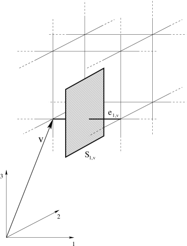
Figure 1: Lattice with elementary edge and surface.

When quantized, holonomies will again become multiplication operators

$$\hat{h}_{I,v}|\ldots,\mu_{I,v},\ldots\rangle=|\ldots,\mu_{I,v}+1,\ldots\rangle$$ (9)

and change the link labels when acting on a state. Note that we do not use a parameter like $\mu_{0}$ since edges of the link size are distinguished and multiplying with holonomies for edges not integer multiples of lattice links does not preserve the lattice structure. The parameter $\mu_{0}$ is thus an integer, simply corresponding to the choice of representation of holonomies. For basic holonomies, $\mu_{0}=1$.

Flux operators

$$\hat{F}_{I,v}|\ldots,\mu_{I,v},\ldots\rangle=\frac{1}{2}\gamma l_{\mathrm{P}}^{2}\mu_{I,v}|\ldots,\mu_{I,v},\ldots\rangle$$ (10)

corresponding to a lattice site orthogonal to an edge in direction $I$ have eigenvalues proportional to $\mu_{I,v}$ or, when we take a surface intersected by the vertex $v$, proportional to the average of labels of neighboring edges,

$$\hat{{\cal F}}_{I,v}|\ldots,\mu_{I,v},\ldots\rangle=\frac{1}{4}\gamma l_{\mathrm{P}}^{2}(\mu_{I,v+e_{I,v}}+\mu_{I,v})|\ldots,\mu_{I,v},\ldots\rangle\,.$$ (11)

In this notation, $v+e_{I,v}$ denotes the vertex next to $v$ along the edge $e_{I,v}$, i.e. the endpoint of $e_{I,v}$ other than $v$. These labels then determine the volume eigenvalues. From

$$V=\int{\mathrm{d}}^{3}x\sqrt{|\tilde{p}^{1}\tilde{p}^{2}\tilde{p}^{3}|}\approx\sum_{v}\ell_{0}^{3}\sqrt{|\tilde{p}^{1}(v)\tilde{p}^{2}(v)\tilde{p}^{3}(v)|}=\sum_{v}\sqrt{|p^{1}(v)p^{2}(v)p^{3}(v)|}$$

the volume operator is defined as $\hat{V}=\sum_{v}\prod_{I=1}^{3}\sqrt{|\hat{\cal F}_{I,v}|}$ with eigenvalues

$$V(\{\mu_{I,v}\})=\left(\frac{\gamma l_{\mathrm{P}}^{2}}{4}\right)^{3/2}\sum_{v}\prod_{I=1}^{3}\sqrt{|\mu_{I,v}+\mu_{I,v+e_{I,v}}|}\,.$$ (12)

Also as in isotropic models, we can construct composite operators such as those for inverse triad components. The only difference is that we construct local versions of such operators localized at vertices, for which we use neighboring link holonomies. Eigenvalues of such commutators will then look similar to those in the isotropic case, except that we have a sum over vertex contributions where single link labels change by $\pm 1$ in the form $V_{v}(\mu_{I,v}+1)-V_{v}(\mu_{I,v}-1)$, rather than one global contribution as in (4). Also, as noted before these functions do not contain $\mu_{0}$ since the link size is fixed. By the same calculations used to derive $d(p)$ in the isotropic case, such functions have peaks at values $\mu_{*}\approx 1$, or $\mu_{*}\approx j$ for an arbitrary irreducible representation, corresponding to $p_{*}\approx\frac{1}{6}\gamma jl_{\mathrm{P}}^{2}$. This is similar to the isotropic case, but now $p_{*}$ distinguishes different regimes according to $\ell_{0}^{2}\tilde{p}>p_{*}$ or $\ell_{0}^{2}\tilde{p}<p_{*}$ rather than inequalities for the isotropic $p=V_{0}^{1/3}\tilde{p}$. So also here, $V_{0}$ has been replaced by the smaller $\ell_{0}$.

4 Basic observations

Having reviewed isotropic basic variables and introduced analogous ones for inhomogeneous lattice states we can draw conclusions regarding their relation. Most of these effects are qualitatively true for any inhomogeneities, but are made explicit in lattice models introduced here.

4.1 Rescaling freedom

As noted before, coordinate background structures to define homogeneity or the choice of lattices in inhomogeneous states introduce parameters such as the cell volume $V_{0}$ or the lattice spacing $\ell_{0}$. The parameters then occur in derived expressions, and such expressions change when other choices for the parameters are made. Since the parameters are related to coordinates or the embedding of structures in space, it is not always guaranteed that such a rescaling freedom makes physical sense. Indeed, for $V_{0}$ this is not the case which is one of the difficulties in purely homogeneous models. Ratios such as $\mu/\mu_{*}=p/p_{*}=V_{0}^{2/3}\tilde{p}/p_{*}$ which demarcate classical from quantum behavior, where $\mu_{*}$ is a characteristic scale appearing in the construction of operators and $\mu$ a state label, depend on $V_{0}$ through $p$. (Factors of $V_{0}$ do not cancel since $p_{*}$ is defined independently of $V_{0}$.)

The situation is, however, different for $\ell_{0}$ which replaces $V_{0}$ in elementary expressions when lattice states are used. Although $V_{0}$ is still present, it always appears in combination with $\ell_{0}$ through $N$. Then, ratios as before take the form $\mu/\mu_{*}=p/p_{*}=\ell_{0}^{2}\tilde{p}/p_{*}$ which is $\ell_{0}$-dependent. But unlike $V_{0}$, changing $\ell_{0}$ has physical meaning because we then change the scale on which we probe space by the lattice. If we choose a bigger lattice spacing, i.e. enlarge $\ell_{0}$, $\tilde{p}$ will have to drop to even smaller values for quantum corrections to become noticeable. Since both $\ell_{0}$ and $\tilde{p}$ are coordinate dependent, this statement about the relation between changing $\ell_{0}$ and corresponding changes in $\tilde{p}$ is invariant under rescaling of coordinates. This happens in such a way that the change of $\ell_{0}$ implies physical properties that are expected. Isotropic models show similar technical features, but due to additional backgrounds involved they are not as physically convincing.

These observations also indicate that the triad scale at which quantum effects become important in inverse powers does not only depend on a representation label chosen for the quantization of inverse triad operators but also on the lattice size. In fact, choosing finer lattices has the same effect as choosing higher representations on a lattice of unchanged size. The importance of such effects is determined by ratios $p/p_{*}$ where $p$ is a flux value and $p_{*}$ is proportional to $j$. Technically, this ratio can be made small by choosing larger $j$, or by making the relevant fluxes take on smaller values in the same situation. In homogeneous settings one only has the first option, while inhomogeneous ones easily allow the second one by choosing smaller surfaces for integrating fluxes.

In fact, if the geometry is nearly isotropic, we can use the average value $p=V_{0}^{2/3}\tilde{p}$ to make contact with isotorpic variables. Now, as discussed at the end of the preceding section, quantum corrections start to become noticeable when $\ell_{0}^{2}\tilde{p}\approx p_{*}$, or $p=V_{0}^{2/3}\tilde{p}=N^{2/3}\ell_{0}^{2}\tilde{p}\approx N^{2/3}p_{*}$ which is enhanced by a factor depending on the number of vertices. Note that we did not use higher representations for holonomies in commutators, by which one can achieve a similar effect if $j\sim N^{2/3}$. The enhancement comes just from the fact that for individual links it is the local value of $\tilde{p}$ rather than the total one which is relevant.

4.2 Higher spin representations

This observation brings us to the next point, which is the naturalness or unnaturalness, or even consistency, of using higher representations of holonomies to construct operators. As we have seen, in inhomogeneous systems one can achieve the same effect by using finer lattices which is certainly a legitimate way to change parameters. While this is not available in homogeneous models, using higher spins there may simply be seen as a way to mimic inhomogeneous behavior in such a setting. There is no direct relation between all features of homogeneous models to the full theory because of degeneracies: changing very different ingredients of an inhomogeneous situation can result in the same change in a homogeneous model. The higher spin compared to the lattice size is one such example, where in earlier papers only the direct relation identifying a higher representation in a homogeneous model with a higher representation in the full theory has been made. If this is the only way to relate higher spins to properties of the full theory, it certainly makes higher spins in homogeneous models look unnatural. The relation to the lattice spacing, overlooked so far, makes using higher representations much more natural in homogeneous models, while inhomogeneous ones can still be formulated by restricting oneself to the fundamental representation in composite operators.

Along similar lines one can justify using different spins for gravitational and matter parts in a Hamiltonian constraint as effective means to include inhomogeneous features. Even if we use higher spins in homogeneous models, one may still question why one should use different ones in holonomies in a matter Hamiltonian compared to the gravitational part of the constraint. Such different spins are often helpful to bring out matter corrections as the dominant ones since they are most easy to derive and to work with. The relation to lattice spacing suggests a reason for higher spins in matter terms compared to gravitational ones: it simply means that for matter terms we use longer range “interactions” based on holonomies which extend through several vertices rather than just one basic lattice link. This is an option one clearly has in any lattice model, for which loop quantum gravity is one example. If one accepts such longer range interactions, one is led directly to the behavior also resulting from higher spins in a homogeneous model.

4.3 Cosmological constant

In addition to ratios $p/p_{*}$ relevant for inverse triad operators, connection components entering holonomies are the second variable which determines where quantum corrections become noticeable. In isotropic models, $\mu_{0}c$ has to be small compared to one for the classical constraint as a polynomial in $c$ to be a good approximation of functions of exponentials $\exp(i\mu_{0}c/2)=\exp(i\mu_{0}V_{0}^{1/3}\tilde{c}/2)$ used for the quantization. As noted before, however, in the presence of a cosmological constant $c$ can become arbitrarily large even in classical regimes (while $\mu_{0}$ has been argued to be of order one by comparing with the lowest area eigenvalue [26]).

In inhomogeneous lattice models, holonomies appearing in composite operators are associated with links and of the form $\exp(i\ell_{0}\tilde{c}/2)=\exp(iN^{-1/3}c/2)$ where we introduced the isotropic $c=V_{0}^{1/3}\tilde{c}$ for comparison. What has to be small is thus not $\mu_{0}c$ but $N^{-1/3}c$ which can be achieved by having a large number of vertices even if $c$ does not become small. A large number of vertices is in fact what one expects if a universe grows to larger size because the fundamental Hamiltonian of loop quantum gravity most likely creates new vertices in its action [31, 32]. The creation of new vertices is not easily incorporated in a regular lattice model, although it is possible, but one can view regular lattices as a coarse-grained, effective description of the fundamental one. For this, no explicit mechanism is required: for effective equations we can compute expansion coefficients locally on a given lattice with $N$ vertices. In those coefficients, metric values appear depending on $N$. Parametrically, $N$ can then be assumed to be a function of the total volume or scale factor whose precise behavior is to be determined by a more detailed formulation. This is analogous to a mean field approximation where “fast” modes are treated only effectively by correction terms. Here, vertices are created at each step of the action of the constraint operator implying Planck-size changes in the local geometry. This degree of freedom is thus much faster than semiclassical effects we are mainly interested in here, i.e. it happens on much smaller time scales (measured in terms of the global geometry).

Then, as the total volume increases one should also adapt the lattice size and increase $N$. This is in particular the case when one has a positive cosmological constant because the universe grows without bound. As the scale factor $a$ increases and $\tilde{c}\propto\sqrt{\Lambda}a$ increases, also $N$ has to increase. For a well-behaved semiclassical state this has to happen in such a way that $c/N^{1/3}$, the argument of holonomies, remains small which is easily achieved in an inhomogeneous model. The validity of a homogeneous model, on the other hand, will break down at a certain volume, which is one example where homogeneous approximations are good on small scales but not at large ones.

We can draw one further conclusion related to this observation. In link holonomies we have the quantity $N^{-1/3}c$ compared to the isotropic $\mu_{0}c$ with a constant $\mu_{0}$. In inhomogeneous situations, $\mu_{0}$ does not appear at all, and there is thus no indication for the makeshift argument relating $\mu_{0}$ to the area spectrum used in the absence of a relation to inhomogeneity. This agrees with the fact that the full constraint operator does not contain the area operator. Curvature components of the constraint are rather quantized directly through holonomies, which is also realized here with natural loops provided by the lattice. Moreover, if $N^{1/3}$ is not treated as a constant, we can resolve problems at large scales. This can be modeled in a purely isotropic situation by letting $\mu_{0}$ be scale-dependent in a form $\bar{\mu}(p)\sim|p|^{-1/2}$ at large scales, corresponding to the number of vertices growing linearly with volume, $N\propto|p|^{3/2}$. This is exactly the behavior which has been proposed within isotropic models to counter large scale and other problems [48, 47]. While one might question a non-constant $\mu_{0}$ in isotropic models on the grounds that holonomies would have to depend on triad variables, the relation to the number of vertices in inhomogeneous states clearly provides convincing justification for it. In general, however, the behavior may differ from $N\propto|p|^{3/2}$ which is to be checked in detailed models implementing the subdivision. There are also conceptual differences between the arguments for $\bar{\mu}(p)$ in isotropic models and those presented here: while in isotropic models the parameter arises at the operator level and leads to holonomies in the constraint depending on triad components, lattice models implement a volume dependence through states. This is closer to the full theory where it is the state-dependent regularization of the Hamiltonian constraint that determines how new edges and vertices are created. Nevertheless, it is promising and encouraging for other constructions in models that independent considerations in homogeneous and inhomogeneous settings lead to the same qualitative conclusions.

4.4 Relative size of quantum corrections

Finally, we discuss the relative size of different quantum corrections arising from quantum Hamiltonians. The main corrections are from inverse triad operators, where the size of $p$ is relevant, and holonomies where $c$ is relevant. While $p$ has to be sufficiently small for inverse triad corrections to become large, $c$ has to be large for large holonomy corrections. For evaluations of effective equations [35, 38, 39, 52, 40, 53] it is then helpful to know if there is any correction which dominates, or if all of them have to be taken together which would make the analysis more complicated. In any model, an answer to this question depends on which regime one is looking at, and the situation in homogeneous models is undecided. Irrespective of what the answer in a particular homogeneous scenario is, however, the situation is different in inhomogeneous models. As before, inhomogeneity implies that for local operators appearing in composite ones connections are integrated only over small links and triads only over lattice sites rather than all of space. Thus, the connection values relevant for holonomies and the triad values for fluxes are both significantly reduced compared to the values that appear in homogenous operators. As a consequence, inverse triad corrections will become more prominent while holonomy corrections will be less so. Main effects are then to be expected from inverse triad corrections of quantum geometry, as they have been studied several times in homogeneous models (see, e.g., [35, 54, 55, 56, 57, 58, 59, 60]).

5 Further applications

Besides these technical observations we can also draw more general conclusions.

5.1 Symmetry reduction: from inhomogeneity to homogeneous models

Symmetric states are obtained by restricting full states to a subset of invariant connections relevant for a symmetric model [10]. Such states are necessarily distributional in the less symmetric situation, and general operators will not leave the space of such states invariant. Nevertheless, one can derive all basic operators given by holonomies and fluxes of the symmetric model from corresponding ones in the full theory. This is sufficient to derive the quantum representation of models from the unique one in the full theory [61, 62]. Since many properties of loop quantizations, including those discussed here, follow already from basic aspects the derivation of the basic representation is a crucial step. Explicit examples for such constructions can be found for reducing an anisotropic model to an isotropic one in [63] and for obtaining the spherically symmetric representation from the full one in [18]. A more general discussion is given in [11].

We can use the constructions presented here to shed more light on the role of inhomogeneities in these reductions. A general lattice state is of the form

$$\psi_{\{\mu_{I,v}\}}[h_{I,v}]=\prod_{I,v}h_{I,v}^{\mu_{I,v}}=\langle k_{J}(x)|\ldots,\mu_{I,v},\ldots\rangle$$

with $k_{I}(x)=\ell_{0}\tilde{k}_{I}(x)$ and $h_{I,v}\approx\exp(i\mu_{I,v}k_{I}(v)/2)$. This corresponds to an isotropic connection $\tilde{c}$ if $\tilde{k}_{I}(x)=\tilde{c}$, or $k_{I}(x)=\ell_{0}V_{0}^{-1/3}c=N^{-1/3}c$, for all $I$ and $x$. The restriction of the state then becomes the isotropic state

$$\psi_{\mu}(c)=\exp(i\mu c/2)=:\langle c|\mu\rangle\quad\mbox{with}\quad\mu=N^{-1/3}\sum_{I,v}\mu_{I,v}\,.$$ (13)

Following the general procedure, there is a map $\sigma$ taking an isotropic state of the reduced model to a distributional state $(\mu|=\sigma(|\mu\rangle)$ in the inhomogeneous setting such that

$$(\mu|\ldots,\mu_{I,v},\ldots\rangle=\langle\mu|\ldots,\mu_{I,v},\ldots\rangle|_{\tilde{k}_{I}(x)=\tilde{c}}\quad\mbox{for all}\quad|\ldots,\mu_{I,v},\ldots\rangle$$ (14)

where the inner product on the right hand side is taken in the isotropic Hilbert space, using the restricted state $|\ldots,\mu_{I,v},\ldots\rangle|_{\tilde{k}_{I}(x)=\tilde{c}}$ as an isotropic state (13).

Link holonomies as multiplication operators simply reduce to multiplication operators on isotropic states. Fluxes for lattice sites, however, do not map isotropic states to other isotropic ones. This can easily be seen using $(\mu|\hat{F}_{J,v^{\prime}}|\ldots,\mu_{I,v},\ldots\rangle=\frac{1}{2}\gamma\ell_{\rm P}^{2}\mu_{J,v^{\prime}}|\ldots,\mu_{I,v},\ldots\rangle$ on states

$$|\psi_{I,v}\rangle:=|0,\ldots,0,1,0,\ldots,0\rangle$$

which have non-zero labels only on one lattice link $e_{I,v}$. We then have

$$(\mu|\hat{F}_{I,v}|\psi_{I,v}\rangle=\frac{1}{2}\gamma\ell_{\rm P}^{2}\mu_{I,v}\delta_{\mu,1}\quad\mbox{and}\quad(\mu|\hat{F}_{I,v}|\psi_{I,v+e_{I,v}}\rangle=0$$

since the flux surface and the non-trivial link do not intersect in the second case. However, $(\nu|\psi_{I,v}\rangle=(\nu|\psi_{I,v+e_{I}}\rangle$ for any isotropic state $(\nu|$. Thus, $(\mu|\hat{F}_{I,v}$ cannot be a superposition of isotropic distributional states, and flux operators associated with a single link do not map the space of isotropic states to itself. (The above formulas show that $(1|$ cannot be contained in a decomposition of $(\mu|\hat{F}_{I,v}$ in basis states, but we can repeat the arguments with arbitrary values for the non-zero label in $|\psi_{I,v}\rangle$.)

Instead, one can use extended fluxes which are closer to homogeneous expressions. First, we extend a lattice site flux $\hat{F}_{I,v}$ to span through a whole plane in the lattice, leading to $\sum_{v^{\prime}:v^{\prime}_{I}=v_{I}}\hat{F}_{I,v^{\prime}}$.

This corresponds to a homogeneous flux in the box of size $V_{0}$ but is still not translationally invariant because the plane $\{v^{\prime}:v^{\prime}_{I}=v_{I}\}$ is distinguished. We can make it homogeneous on the lattice by averaging along the direction $I$ transversal to the plane. This leads to a sum over all lattice vertices in

$$\hat{p}^{I}:=N^{-1/3}\sum_{v}\hat{F}_{I,v}$$

including a factor $N^{-1/3}$ from averaging in one direction. Finally, we take the directional average

$$\hat{p}=\frac{1}{3}\sum_{I}\hat{p}^{I}=\frac{1}{3N^{1/3}}\sum_{I,v}\hat{F}_{I,v}$$

to define the isotropic flux operator.

Now, to find the action of this operator on a distributional state $(\nu|$ we compute

$$(\nu|\hat{p}|\ldots,\mu_{I,v},\ldots\rangle=\frac{\gamma\ell_{\rm P}^{2}}{6N^{1/3}}\sum_{J,v^{\prime}}\mu_{J,v^{\prime}}(\nu|\ldots,\mu_{I,v},\ldots\rangle=\frac{1}{6}\gamma\ell_{\rm P}^{2}\mu\delta_{\nu,\mu}$$

where $\mu$ is defined in terms of $\mu_{I,v}$ as in (13). This agrees with the isotropic flux operator defined in isotropic models,

$$\hat{p}\sigma(|\mu\rangle)=\sigma(\hat{p}|\mu\rangle)\,,$$ (15)

and shows in particular that $\hat{p}$, unlike $\hat{p}_{I,v}$, maps an isotropic distribution to another such state. Thus, the isotropic representation in loop quantum cosmology follows from the inhomogeneous one along the lines of a symmetry reduction at the quantum level. Notice that this leads directly to an operator for $p$ rather than $\tilde{p}$ without explicitly introducing the cell size $V_{0}$. We just extend fluxes over the whole lattice in order to make them homogeneous, such that the combination $V_{0}^{2/3}\tilde{p}=p$ automatically arises.

5.2 Gravitons as collective excitations

On inhomogeneous lattice states we can look for representations of inhomogeneous excitations of geometry. Classically, such excitations are given by modes of a metric perturbation $q_{ab}=\bar{q}_{ab}+h_{ab}$ on a background $\bar{q}_{ab}$. In a perturbative quantization on that background, $h_{ab}$ would thus be the basic field to be quantized, leading to the expectation of one-particle states called gravitons corresponding to transverse-traceless modes of $h_{ab}$.

In loop quantum gravity, the situation is different because its basic formulation is background independent. Having formulated here a lattice description as a sector which re-introduces a metric background, we can see how such metric perturbations are realized. Simplifications due to Abelianization used here also occur in constructions of explicit states in linearized gravity [67]. As in the full theory, basic excitations of the loop quantization are given by dynamical moves which change the labels $\mu_{I,v}$ locally at a vertex to $\mu_{I,v}\pm 1$. This changes the local labels, corresponding to inhomogeneous modes, but also the total volume corresponding to the background volume of $\bar{q}_{ab}$. A quantum analog of the mode can be defined as the difference

$$\delta p_{I,v}=p_{I,v}-\bar{p}=\frac{1}{2}\gamma\ell_{\rm P}^{2}\mu_{I,v}-(V(\{\mu_{I,v}\})/N)^{2/3}$$

between local labels and the average volume which captures properties of the classical modes even at the level of effective dynamics [21].

The quantum picture of these excitation is then very different from the classical one: $\delta p_{I,v}$ arises non-locally since we have to sum over the whole lattice to subtract off the background. Basic dynamical moves of the quantum theory change the local quantum excitation as well as the background, leading to a mode change also in a non-local way. In this picture, metric modes such as gravitons arise as collective excitations out of the underlying lattice formulation: many basic quantum modes combine to give classical excitations.

5.3 Quantum gravity corrections for large universes

Quantum expressions differing from their classical analogs give rise to corrections to classical equations. This usually occurs on small length or large curvature scales as they are realized in the very early universe. But subdivision in a lattice also makes relevant local length scales smaller, and indeed we already noticed that inverse power corrections as functions of $p^{I}(v)$ become dominant over holonomy corrections because the flux values are reduced on lattice links if the lattice becomes finer. This opens the possibility for small corrections on single lattice sites to add up to sizeable corrections on the whole lattice, which can influence the evolution of modes [21] or even of the whole universe.

6 Conclusions

Models of loop quantum gravity are being investigated actively regarding their phenomenological properties, and perturbative inhomogeneities are currently being included. This brings us closer to reliable computations of potentially observable properties such as those of structure formation. It is then important to check all intrinsic details of such models and see how faithfully they incorporate features of the full theory. As we discussed, qualitative effects are realized in homogeneous as well as inhomogeneous lattice models in the same way. We introduced inhomogeneous lattice constructions in a way which allows for a relation to a homogeneous background. The relation to isotropic models is then clear, which provides a new step toward relating isotropic models to the full theory. Although the lattice construction is analogous to that of isotropic models, quantitative aspects can change which has a bearing on which ranges of parameters one considers as natural or unnatural. It also plays a role for which correction terms will be dominant in different regimes which is the most important aspect for phenomenological investigations.

The lattices used here are not intended as fundamental descriptions since they are not background independent. They are rather to be thought of as effective lattice models which result if some degrees of freedom of the full theory are interpreted as providing a background for other degrees of freedom. This simplifies the more irregular fundamental behavior. It is this feature which helps to illustrate and clarify some puzzling properties realized in isotropic models. There are also further applications such as explicit constructions of quantum field theories on a quantum spacetime as suggested in [68, 66], more general models for field propagation with quantum corrections based on [65], or cosmological perturbations [21]. Such lattice models are more accessible for a relation to the full theory and can thus be used to suggest relevant properties which one wants to ensure in future constructions and specifications of the full theory at a basic level.

For now, the construction already presents several applications. They all rely on the re-introduction of a background which is necessary to interpret computational results. We focused here on kinematical aspects, but an inclusion of characteristic dynamical ones is in progress. For a detailed description of all effects expected in fully inhomogeneous settings, remaining difficulties are an explicit treatment of subdivision and the inclusion of non-Abelian properties. But this is not required explicitly for effective perturbations where the lattice description discussed here is sufficient. It allows one to derive perturbation equations for metric modes around the background, to be used for instance for cosmological structure formation, or to understand the emergence of graviton states conceptually.

Note added: After this paper had been submitted to the journal General Relativity and Gravitation, the preprint gr-qc/0607100 by Kristina Giesel and Thomas Thiemann was posted. Although the conceptual setup is quite different from the approach followed here, it is clear that there is a convergence of different ideas pursued recently in loop quantum gravity. Especially in combination with the results of Sec. 5.1, there is now close contact between the full theory (understood as a general framework to set up background independent quantum kinematics and dynamics without symmetry assumptions) and loop quantum cosmology.

References

- [1] C. Rovelli, Quantum Gravity, Cambridge University Press, Cambridge, UK, 2004
- [2] A. Ashtekar and J. Lewandowski, Background independent quantum gravity: A status report, Class. Quantum Grav. 21 (2004) R53–R152, [gr-qc/0404018]
- [3] T. Thiemann, Introduction to Modern Canonical Quantum General Relativity, [gr-qc/0110034]
- [4] C. Rovelli and L. Smolin, Discreteness of Area and Volume in Quantum Gravity, Nucl. Phys. B 442 (1995) 593–619, [gr-qc/9411005], Erratum: Nucl. Phys. B 456 (1995) 753
- [5] A. Ashtekar and J. Lewandowski, Quantum Theory of Geometry I: Area Operators, Class. Quantum Grav. 14 (1997) A55–A82, [gr-qc/9602046]
- [6] A. Ashtekar and J. Lewandowski, Quantum Theory of Geometry II: Volume Operators, Adv. Theor. Math. Phys. 1 (1997) 388–429, [gr-qc/9711031]
- [7] M. Bojowald, Absence of a Singularity in Loop Quantum Cosmology, Phys. Rev. Lett. 86 (2001) 5227–5230, [gr-qc/0102069]
- [8] A. Ashtekar and M. Bojowald, Quantum Geometry and the Schwarzschild Singularity, Class. Quantum Grav. 23 (2006) 391–411, [gr-qc/0509075]
- [9] M. Bojowald, Non-singular black holes and degrees of freedom in quantum gravity, Phys. Rev. Lett. 95 (2005) 061301, [gr-qc/0506128]
- [10] M. Bojowald and H. A. Kastrup, Symmetry Reduction for Quantized Diffeomorphism Invariant Theories of Connections, Class. Quantum Grav. 17 (2000) 3009–3043, [hep-th/9907042]
- [11] M. Bojowald, Loop Quantum Cosmology, Living Rev. Relativity 8 (2005) 11, [gr-qc/0601085], http://relativity.livingreviews.org/Articles/lrr-2005-11/
- [12] A. Ashtekar, J. C. Baez, A. Corichi, and K. Krasnov, Quantum Geometry and Black Hole Entropy, Phys. Rev. Lett. 80 (1998) 904–907, [gr-qc/9710007]
- [13] A. Ashtekar, J. C. Baez, and K. Krasnov, Quantum Geometry of Isolated Horizons and Black Hole Entropy, Adv. Theor. Math. Phys. 4 (2000) 1–94, [gr-qc/0005126]
- [14] C. Rovelli, Graviton propagator from background-independent quantum gravity, [gr-qc/0508124]
- [15] G. Ellis, Relativistic cosmology: its nature, aims and problems, In: General Relativity and Gravitation, Ed.: Bertotti, B. et al., pp. 215–288, Reidel, 1984
- [16] M. Bojowald, Degenerate Configurations, Singularities and the Non-Abelian Nature of Loop Quantum Gravity, Class. Quantum Grav. 23 (2006) 987–1008, [gr-qc/0508118]
- [17] A. S. Eddington, The Philosophy of Physical Science, The Macmillan company, Cambridge, 1939 (translated back from the German edition)
- [18] M. Bojowald, Spherically Symmetric Quantum Geometry: States and Basic Operators, Class. Quantum Grav. 21 (2004) 3733–3753, [gr-qc/0407017]
- [19] M. Bojowald and R. Swiderski, The Volume Operator in Spherically Symmetric Quantum Geometry, Class. Quantum Grav. 21 (2004) 4881–4900, [gr-qc/0407018]
- [20] M. Bojowald and R. Swiderski, Spherically Symmetric Quantum Geometry: Hamiltonian Constraint, Class. Quantum Grav. 23 (2006) 2129–2154, [gr-qc/0511108]
- [21] M. Bojowald, H. Hernández, M. Kagan, P. Singh, and A. Skirzewski, to appear
- [22] A. Ashtekar, New Hamiltonian Formulation of General Relativity, Phys. Rev. D 36 (1987) 1587–1602
- [23] J. F. Barbero G., Real Ashtekar Variables for Lorentzian Signature Space-Times, Phys. Rev. D 51 (1995) 5507–5510, [gr-qc/9410014]
- [24] M. Bojowald, Isotropic Loop Quantum Cosmology, Class. Quantum Grav. 19 (2002) 2717–2741, [gr-qc/0202077]
- [25] G. Immirzi, Real and Complex Connections for Canonical Gravity, Class. Quantum Grav. 14 (1997) L177–L181
- [26] A. Ashtekar, M. Bojowald, and J. Lewandowski, Mathematical structure of loop quantum cosmology, Adv. Theor. Math. Phys. 7 (2003) 233–268, [gr-qc/0304074]
- [27] T. Thiemann, QSD V: Quantum Gravity as the Natural Regulator of Matter Quantum Field Theories, Class. Quantum Grav. 15 (1998) 1281–1314, [gr-qc/9705019]
- [28] M. Bojowald, Inverse Scale Factor in Isotropic Quantum Geometry, Phys. Rev. D 64 (2001) 084018, [gr-qc/0105067]
- [29] M. Bojowald, Quantization ambiguities in isotropic quantum geometry, Class. Quantum Grav. 19 (2002) 5113–5130, [gr-qc/0206053]
- [30] M. Bojowald, Loop Quantum Cosmology: Recent Progress, In Proceedings of the International Conference on Gravitation and Cosmology (ICGC 2004), Cochin, India, Pramana 63 (2004) 765–776, [gr-qc/0402053]
- [31] C. Rovelli and L. Smolin, The physical Hamiltonian in nonperturbative quantum gravity, Phys. Rev. Lett. 72 (1994) 446–449, [gr-qc/9308002]
- [32] T. Thiemann, Quantum Spin Dynamics (QSD), Class. Quantum Grav. 15 (1998) 839–873, [gr-qc/9606089]
- [33] M. Gaul and C. Rovelli, A generalized Hamiltonian Constraint Operator in Loop Quantum Gravity and its simplest Euclidean Matrix Elements, Class. Quantum Grav. 18 (2001) 1593–1624, [gr-qc/0011106]
- [34] K. Vandersloot, On the Hamiltonian Constraint of Loop Quantum Cosmology, Phys. Rev. D 71 (2005) 103506, [gr-qc/0502082]
- [35] M. Bojowald, Inflation from quantum geometry, Phys. Rev. Lett. 89 (2002) 261301, [gr-qc/0206054]
- [36] M. Bojowald and K. Vandersloot, Loop quantum cosmology, boundary proposals, and inflation, Phys. Rev. D 67 (2003) 124023, [gr-qc/0303072]
- [37] P. Singh and K. Vandersloot, Semi-classical States, Effective Dynamics and Classical Emergence in Loop Quantum Cosmology, Phys. Rev. D 72 (2005) 084004, [gr-qc/0507029]
- [38] K. Banerjee and G. Date, Discreteness Corrections to the Effective Hamiltonian of Isotropic Loop Quantum Cosmology, Class. Quant. Grav. 22 (2005) 2017–2033, [gr-qc/0501102]
- [39] J. Willis, On the Low-Energy Ramifications and a Mathematical Extension of Loop Quantum Gravity, PhD thesis, The Pennsylvania State University, 2004
- [40] M. Bojowald and A. Skirzewski, Quantum Gravity and Higher Curvature Actions, In Current Mathematical Topics in Gravitation and Cosmology (42nd Karpacz Winter School of Theoretical Physics), [hep-th/0606232]
- [41] M. Bojowald, J. E. Lidsey, D. J. Mulryne, P. Singh, and R. Tavakol, Inflationary Cosmology and Quantization Ambiguities in Semi-Classical Loop Quantum Gravity, Phys. Rev. D 70 (2004) 043530, [gr-qc/0403106]
- [42] A. Perez, On the regularization ambiguities in loop quantum gravity, Phys. Rev. D 73 (2006) 044007, [gr-qc/0509118]
- [43] M. Bojowald and A. Rej, Asymptotic Properties of Difference Equations for Isotropic Loop Quantum Cosmology, Class. Quantum Grav. 22 (2005) 3399–3420, [gr-qc/0504100]
- [44] J. Rosen, J.-H. Jung and G. Khanna, Instabilities in numerical loop quantum cosmology, [gr-qc/0607044]
- [45] G. Date and G. M. Hossain, Effective Hamiltonian for Isotropic Loop Quantum Cosmology, Class. Quantum Grav. 21 (2004) 4941–4953, [gr-qc/0407073]
- [46] G. Date and G. M. Hossain, Genericity of Big Bounce in isotropic loop quantum cosmology, Phys. Rev. Lett. 94 (2005) 011302, [gr-qc/0407074]
- [47] A. Ashtekar, T. Pawlowski, and P. Singh, Quantum Nature of the Big Bang: Improved dynamics, [gr-qc/0607039]
- [48] P. Singh, Loop cosmological dynamics and dualities with Randall-Sundrum braneworlds, Phys. Rev. D 73 (2006) 063508, [gr-qc/0603043]
- [49] A. Ashtekar, J. Lewandowski, D. Marolf, J. Mourão, and T. Thiemann, Quantization of Diffeomorphism Invariant Theories of Connections with Local Degrees of Freedom, J. Math. Phys. 36 (1995) 6456–6493, [gr-qc/9504018]
- [50] M. Bojowald, Loop Quantum Cosmology: I. Kinematics, Class. Quantum Grav. 17 (2000) 1489–1508, [gr-qc/9910103]
- [51] M. Bojowald, Loop Quantum Cosmology: II. Volume Operators, Class. Quantum Grav. 17 (2000) 1509–1526, [gr-qc/9910104]
- [52] M. Bojowald and A. Skirzewski, Effective Equations of Motion for Quantum Systems, Rev. Math. Phys., to appear, [math–ph/0511043]
- [53] A. Ashtekar, M. Bojowald, and J. Willis, in preparation
- [54] P. Singh and A. Toporensky, Big Crunch Avoidance in Semi-Classical Loop Quantum Cosmology, Phys. Rev. D 69 (2004) 104008, [gr-qc/0312110]
- [55] G. V. Vereshchagin, Qualitative Approach to Semi-Classical Loop Quantum Cosmology, JCAP 07 (2004) 013, [gr-qc/0406108]
- [56] J. E. Lidsey, D. J. Mulryne, N. J. Nunes, and R. Tavakol, Oscillatory Universes in Loop Quantum Cosmology and Initial Conditions for Inflation, Phys. Rev. D 70 (2004) 063521, [gr-qc/0406042]
- [57] N. J. Nunes, Inflation: A graceful entrance from Loop Quantum Cosmology, Phys. Rev. D 72 (2005) 103510, [astro-ph/0507683]
- [58] M. Bojowald and G. Date, Quantum suppression of the generic chaotic behavior close to cosmological singularities, Phys. Rev. Lett. 92 (2004) 071302, [gr-qc/0311003]
- [59] M. Bojowald, R. Maartens, and P. Singh, Loop Quantum Gravity and the Cyclic Universe, Phys. Rev. D 70 (2004) 083517, [hep-th/0407115]
- [60] M. Bojowald, R. Goswami, R. Maartens, and P. Singh, A black hole mass threshold from non-singular quantum gravitational collapse, Phys. Rev. Lett. 95 (2005) 091302, [gr-qc/0503041]
- [61] J. Lewandowski, A. Okołów, H. Sahlmann, and T. Thieman, Uniqueness of diffeomorphism invariant states on holonomy-flux algebras, [gr-qc/0504147]
- [62] C. Fleischhack, Representations of the Weyl Algebra in Quantum Geometry, [math-ph/0407006]
- [63] M. Bojowald, H. H. Hernández, and H. A. Morales-Técotl, Perturbative degrees of freedom in loop quantum gravity: Anisotropies, Class. Quantum Grav. 23 (2006) 3491–3516, [gr-qc/0511058]
- [64] H. Sahlmann, T. Thiemann and O. Winkler, Coherent States for Canonical Quantum General Relativity and the Infinite Tensor Product Extension, Nucl. Phys. B 606 (2001) 401–440, [gr-qc/0102038]
- [65] M. Bojowald, H. Morales-Técotl, and H. Sahlmann, On Loop Quantum Gravity Phenomenology and the Issue of Lorentz Invariance, Phys. Rev. D 71 (2005) 084012, [gr-qc/0411101]
- [66] H. Sahlmann and T. Thiemann, Towards the QFT on Curved Spacetime Limit of QGR. II: A Concrete Implementation, Class. Quantum Grav. 23 (2006) 909–954, [gr-qc/0207031]
- [67] M. Varadarajan, Gravitons from a loop representation of linearised gravity, Phys. Rev. D 66 (2002) 024017, [gr-qc/0204067]
- [68] H. Sahlmann and T. Thiemann, Towards the QFT on Curved Spacetime Limit of QGR. I: A General Scheme, Class. Quantum Grav. 23 (2006) 867–908, [gr-qc/0207030]