Quasinormal modes for the Vaidya metric

Abstract

We consider here scalar and electromagnetic perturbations for the Vaidya metric in double-null coordinates. Such an approach allows one to go a step further in the analysis of quasinormal modes for time-dependent spacetimes. Some recent results are refined, and a new non-stationary behavior corresponding to some sort of inertia for quasinormal modes is identified. Our conclusions can enlighten some aspects of the wave scattering by black holes undergoing some mass accretion processes.

I Introduction

The quasinormal modes analysis is a paradigm for the study of gravitational excitations of black holes. For a comprehensive review on the vast previous literature, see Nellert-99 ; Kokkotas-99 . We stress that the quasinormal modes (QNM) of black holes are also experimentally relevant since they could, in principle, be detected in gravitational waves detector such as LISA (see, for instance, berti05 and references therein). The robustness of QNM analysis has been established by considering several kinds of generalizations, as, for instance, relaxing the asymptotic flatness conditionBrady-97 ; Molina-04 ; Du-04 or considering time-dependent situationsHod-02 ; Xue-04 ; Cheng-04 . The case of asymptotic Anti-de-Sitter black holes has deserved special attention due to its relevance to the AdS/CFT conjectureChan-97 ; Cardoso-124015 ; Horowitz-00 ; Wang-00 ; Wang-01 ; Cardoso-084017 ; Berti-03 ; Konoplya-02 ; Birmingham-02 ; Zhu-01 ; Musiri-03 ; Cardoso-084020 ; Cardoso-03 .

The analysis of QNM for time-dependent situations is of special physical interest since it is expect that a black hole can enlarge its mass by some accretion process, or even lose mass by some other process, including Hawking radiation. The late time tail for a Klein Gordon field under a time-dependent potential was first considered in Hod-02 , where some influence of the temporal dependence of the potential over the characteristic decaying tails was reported. Such a kind of time-dependent potential arises naturally when the Vaidya metric is consideredXue-04 ; Cheng-04 . The Vaidya metric, which in radiation coordinates $(w,r,\theta,\phi)$ has the form

$$ds^{2}=-\left(1-\frac{2m(w)}{r}\right)dw^{2}+2cdrdw+r^{2}d\Omega^{2},$$ (1)

where $d\Omega^{2}=d\theta^{2}+\sin^{2}\theta d\phi^{2}$, $c=\pm 1$, is a solution of Einstein’s equations with spherical symmetry in the eikonal approximation to a radial flow of unpolarized radiation. For the case of an ingoing radial flow, $c=1$ and $m(w)$ is a monotone increasing mass function in the advanced time $w$, while $c=-1$ corresponds to an outgoing radial flow, with $m(w)$ being in this case a monotone decreasing mass function in the retarded time $w$. The metric (1) is the starting point for the QNM analysis of varying mass black-holes.

In Cheng-04 , massless scalar fields were studied on an electrically charged version of the Vaidya metric. Basically, two kinds of continuously varying mass functions were considered:

$$m(w)=\left\{{{\begin{array}[]{l l}{m_{1}}&{w\leq w_{1}},\\ {m_{1}}f(w)&{w_{1}\leq w\leq w_{2}},\\ {m_{2}}&{w\geq w_{2}},\\ \end{array}}}\right.\\$$ (2)

with $f(w)=(1-\lambda w)$ and $f(w)=\exp{(-\alpha w)}$, called, respectively, linear and exponential models. Generalized tortoise coordinates were introduced, and a standard numerical analysis was done. The conclusion was that, as a first approximation, the QNM for a stationary Reissner-Nordström black hole with mass $m(w)$ and charge $q(w)=q_{0}m(w)$ are still valid, as if some stationary adiabatic regime was indeed governing the QNM dynamics for time-dependent spacetimes. In principle, one should not expect such stationary behavior for very rapid varying mass functions, however the analysis of Cheng-04 was not able to identify any breaking of such an adiabatic regime. We notice also that both linear and exponential models, inspired by some known exact solutionsWL for which generalized tortoise coordinates could be explicitly constructed, would hardly correspond to physically realistic cases. Both cases have $C^{0}$-class mass functions, implying the existence of some infinitesimal shell distributions of matters for $w=w_{0}$ and $w=w_{1}$ whose interpretation and role are still unclear.

We attack here the QNM problem by considering the Vaidya metric in double-null coordinatesGS . The main advantage of such an approach is the possibility of considering any (monotone) mass function, allowing, for instance, the analysis of smooth mass functions that could correspond to physically more relevant situations, free of obscure infinitesimal matter shells. Furthermore, the use of double-null coordinates has improved considerably the overall precision of the numerical analysis, allowing us to identify the breakdown of the adiabatic regime, characterized by the appearing of a non-stationary inertial effect for the QNM in the case of rapid varying mass functions. Once the stationary regime is reached, the standard QNM results hold, reinforcing, once more, the robustness of the QNM analysis. Our results can be used as a first approximation to describe the propagation of small perturbations around astrophysically realistic situations where black holes undergo some mass accretion processes. We notice that the non-stationary inertial effect presented here is in perfect agreement with the non-linear analysis preformed in Zlochower:2003yh , which reported extra redshift effects on the QNM frequencies due to the growth of the effective black hole mass.

We organize this paper as follows. The next section is devoted to a brief introduction to the semi-analytical approachGS for the Vaidya metric in double-null coordinates. Section III presents the main issues and results of our numerical analysis. The last section is left to some closing remarks.

II The Vaidya metric in double-null coordinates

Double-null coordinates are specially suitable for time-evolution problems as the QNM analysis. However, the difficulties of constructing double-null coordinates for non-stationary spacetime are well known. The Vaidya metric is a typical example (see GS and references therein). Indeed, it is known that the problem of constructing double-null coordinates for generic mass functions is not analytical soluble in generalWL . The semi-analytical approach proposed in GS is the starting point for our analysis here. It consists, basically, in considering the Vaidya metric in double-null coordinates ab initio, avoiding the need of constructing any coordinate transformation. The spherically symmetric line element in double-null coordinates is

$$ds^{2}=-2f(u,v)du\,dv+r^{2}(u,v)d\Omega^{2},$$ (3)

where $f(u,v)$ and $r(u,v)$ are smooth non vanishing functions. The energy-momentum tensor of a unidirectional radial flow of unpolarized radiation in the eikonal approximation is given by

$$T_{ab}=\frac{1}{8\pi}h(u,v)k_{a}k_{b},$$ (4)

where $k_{a}$ is a radial null vector. The Einstein’s equations for the case of a flow in the $v$-direction can then be reduced to the following set of equationsWL ; GS

$$f(u,v) = 2B(v)\partial_{u}r(u,v),$$ (5)

$$\partial_{v}r(u,v) = -B(v)\left(1-\frac{2m(v)}{r(u,v)}\right),$$ (6)

$$h(u,v) = -4\frac{B(v)m^{\prime}(v)}{r^{2}(u,v)},$$ (7)

where $B(v)$ and $m(v)$ are arbitrary functions obeying, according to the weak energy condition,

$$B(v)m^{\prime}(v)\leq 0,$$ (8)

where the prime denotes the derivative with respect to $v$. The solution of (5)-(7) will correspond to the Vaidya metric in double-null coordinates, as one can interpret from (3) and (4). For $m^{\prime}(v)\neq 0$, the choice

$$B=-\frac{1}{2}{\rm sign}(m^{\prime})$$ (9)

allows one to interpret $m(v)$ as the mass of the solution and $v$ as the proper time as measured in the rest frame at infinity for the asymptotically flat caseWL ; GS . Note that if the weak energy condition (8) holds, the function $m(v)$ is monotone, implying that the radial flow must be ingoing or outgoing for all $v$. It is not possible, for instance, to have “oscillating” mass functions $m(v)$.

The semi-analytical approach of GS consists in a strategy to construct numerically the functions $f(u,v)$, $r(u,v)$ and $h(u,v)$ from the Eq. (5)-(7), and to infer the underlying causal structure. Eq. (6) along $u$ constant is a first order ordinary differential equation in $v$. One can evaluate the function $r(u,v)$ in any point by solving the $v$-initial value problem knowing $r(u,v_{0})$. The trivial example of Minkowski spacetime ($m=0$), for instance, can be obtainedGS by choosing $r(u,0)=u/2$. Once we have $r(u,v)$, we can evaluate $f(u,v)$ and $h(u,v)$ from (5) and (7). Further details of the method can be found in GS . We consider here the following smooth mass function

$$m(v)=m_{1}+\frac{m_{2}-m_{1}}{2}\left[1+\tanh\rho(v-v_{1})\right]$$ (10)

where $\rho$ and $v_{1}$ are also constant parameters. For sake of comparison with the results of Cheng-04 , we also consider a linear model. Fig. 1 depicts the causal structure corresponding to the hyperbolic mass

Figure 1: Lines of constant $u$ for the solution of (6) with the hyperbolic mass function (10), with $m_{2}>m_{1}$ and $\rho>0$. All solutions in the region below the line $r=2m(v)$ (the apparent horizon) have $r^{\prime}<0$, where the prime denotes the derivative with respect to $v$. Any solution that enters into this region will reach the singularity at $r=0$ with finite $v$. On the other hand, solutions confined to the $r^{\prime}>0$ region always escape from the singularity and reach ${\cal I^{+}}$. In the present case, there exists an event horizon (the dashed line on the inserted conformal diagram) close to the solutions $r_{\rm H}(v)$.

function (10) obtained from the semi-analytical approach. For positive $\rho$ and $m_{2}>m_{1}$, for instance, it represents a black hole with mass $m_{1}$ receiving a radial flux of radiation and, consequently, enlarging continuously its mass until reaching $m_{2}$. The choice of the initial condition for solving (6) is a rather subtle issueGS . For our purposes here, we note only that demanding $\partial_{u}r(u,v_{0})\neq 0$ is sufficient to guarantee that, for any $m(v)$, the underlying spacetime causal structure does not depend on the initial condition $r(u,v_{0})$. For constant $m$ and $B=-1/2$, Eq. (6) can be easily integrated, leading to

$$r(u,v)+2m\ln|r(u,v)-2m|-\frac{v}{2}=P(u),$$ (11)

where $P(u)$ is an arbitrary function of $u$. It is also possible to solve Eq. (6) analytically for the linear and exponential mass functionsWL . Eq. (11) is our reference to choose the initial conditions $r(u,v_{0})$.

III Scalar and electromagnetic perturbations

In the coordinate system (3), for any desired form of the mass function $m(v)$, the equations for scalar and electromagnetic perturbations can be easily put in the formKokkotas-99

$$\frac{\partial^{2}\psi}{\partial u\partial v}+V(u,v)f(u,v)\psi=0,$$ (12)

where the potential $V(u,v)$ is given by

$$V(u,v)=\frac{\ell(\ell+1)}{2r^{2}(u,v)}+\sigma\frac{m(v)}{r^{3}(u,v)},$$ (13)

where $\sigma=1$ and $\sigma=0$ correspond, respectively, to the scalar and to the electromagnetic cases. For a given mass function $m(v)$, one first evaluates the function $f(u,v)$ and $r(u,v)$ with the semi-analytical approach of the previous section, and then the characteristic problem corresponding to (12) can be solved with the usual second order characteristic algorithmKokkotas-99 , where the initial data are specified along the two null surfaces $u=u_{0}$ and $v=v_{0}$. Since the basic aspects of the field decay are independent of the initial conditions (this fact is confirmed by our simulations), we use the Gaussian initial condition

$$\psi(u=u_{0},v)=\exp\left[-\frac{(v-v_{c})^{2}}{2\sigma^{2}}\right]\ ,$$ (14)

and $\psi(u,v=v_{0})=\rm const$. Our typical numerical grid is large enough to assure that we can set effectively this last constant to zero. After the integration is completed, the values $\psi(u_{max},v)$ are extracted, where $u_{max}$ is the maximum value of $u$ on the numerical grid. Taking sufficiently large $u_{max}$, we have good

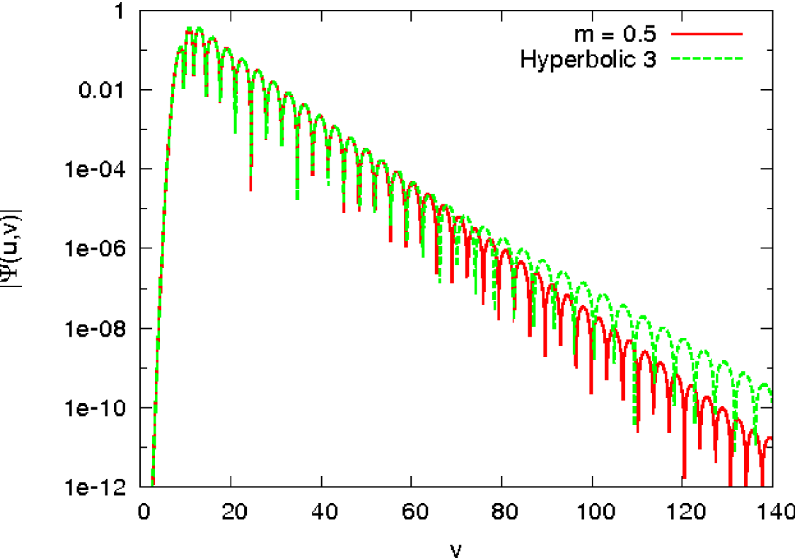
Figure 2: Values of the electromagnetic perturbations $\psi(u_{max},v)$ with $\ell=2$ for a Schwarzschild black hole with mass $m=0.5$ and for the Vaidya metric with the hyperbolic mass function (10), where $v_{1}=75$, $\rho=0.08$, $m_{1}=0.5$, and $m_{2}=0.65$ (Hyperbolic 3). One can clearly appreciate, for the time-dependent case, the slowing down of the oscillation frequency and damping taking place after $v_{1}$.

approximations for the wave function at the event horizon. Figure 2 presents an example of $\psi(u_{max},v)$ data for a hyperbolic increasing mass function and its comparison with the case of a Schwarzschild black hole. Similar results hold if we extract the data for other values of $u$. All the analysis presented here corresponds to the data extracted on the horizon $u_{max}$. Note that the choice of $u_{max}$ is a matter of numerical convenience. Since the QNM corresponds to eigenstates of an effective Schroedinger equationKokkotas-99 , the associated complex eigenvalues can be read out anywhere once the asymptotic regime is attained.

From the function $\psi(u_{max},v)$, one can infer the characteristic frequencies $\omega$ of the damped oscillating modes. Since the frequencies $\omega$ are themselves time-dependent (see Fig. 2), for a given $v$, $\omega(v)$ is determined locally by a non-linear $\chi^{2}$-fitting by using some damped cycles of $\psi$ around $v$.

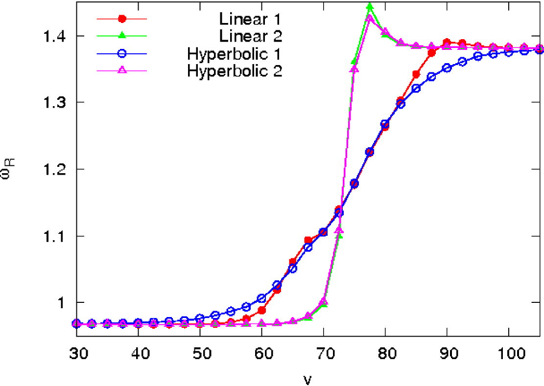
Figure 3: The real ($\omega_{\rm R}$) part of the frequency for scalar perturbations with $\ell=2$ as function of $v$ for decreasing linear and hyperbolic mass functions. For all the cases, $m_{1}=0.5$ and $m_{2}=0.35$. Linear 1: $v_{1}=60$, $v_{2}=90$. Linear 2: $v_{1}=74.5$, $v_{2}=75.5$. Hyperbolic 1: $v_{1}=75$, $\rho=0.08$. Hyperbolic 2: $v_{1}=75$, $\rho=0.8$. The imaginary part $\omega_{\rm I}$ has similar behavior as for the increasing mass case (Fig. 4), see the text.

We perform an exhaustive numerical analysis for many different mass functions $m(v)$. Figures 3 and 4 present the real ($\omega_{\rm R}$) and imaginary ($\omega_{\rm I}$) part of the frequencies of the perturbations as function of $v$. They correspond, respectively, to some decreasing and increasing mass functions, and are typical for all values of $\ell$, all kinds of perturbations (scalar and electromagnetic) and different initial conditions. The imaginary part $\omega_{\rm I}$ exhibits similar time-dependence, although its values are typically known with lower precision than $\omega_{\rm R}$. This is not, however, due to numerical errors in the integration procedure. In fact, the convergence of the second order characteristic algorithm is quite good. For instance, the differences in the calculated frequencies of Fig. 3 and 4 obtained by using as integration steps $\Delta u=\Delta v=0.2,0.1,$ and 0.05, are smaller than the size of the points used in the figures, and no difference is detected for even smaller steps. We credit the irregularities observed for $\omega_{\rm I}$ to the local $\chi^{2}$-fitting described above. For subcritical damped oscillations as the QNM considered here, the oscillation frequencies $\omega_{\rm R}$ can be easily determined from a few damped cycles, while for the damping term $\omega_{\rm I}$ one typically needs many more cycles in order to get a similar precision. By taking a large number of cycles we will tend to smear the calculated frequencies, leading to some kind of average and not to the desired instantaneous values. We opt, then, to take as few as possible cycles, paying the price of having some irregularities for $\omega_{\rm I}$.

Let us take for a close analysis, for instance, the case of decreasing $m(v)$ (Fig. 3). For the rapid varying cases (Linear 2 and Hyperbolic 2), one clearly sees the inertial effect for $\omega_{\rm R}$ near $v=75$. The function $\omega_{\rm R}(v)$ does not follow the track corresponding to $m^{-1}(v)$, as one would expect for a stationary adiabatic regime, and as it really does for the Hyperbolic 1 case. After the rapid increasing phase, $\omega_{\rm R}$ acts as it would have some intrinsic inertia, reaching a maximum value that is bigger than $\omega_{\rm R}(\infty)$, implying the relaxation corresponding to the region with $\omega^{\prime}_{\rm R}(v)<0$ for $v>75$. We also notice that, for the rapid varying case, one could not detect sensible differences between the smooth hyperbolic case and the $C^{0}$ linear one. Nevertheless, one can see that the slower linear case (Linear 1) exhibits some inertial effects close the the second matching point of $m(v)$. In all other regions, it follows the track corresponding to $m^{-1}(v)$. No appreciable difference in the transients of scalar and electromagnetic perturbations was detected. As we have already mentioned, such transient inertial behavior passed unnoticed by the QNM analysis in radiation coordinates performed in Cheng-04 . Analogous conclusions hold for the case of increasing $m(v)$ (Fig. 4).

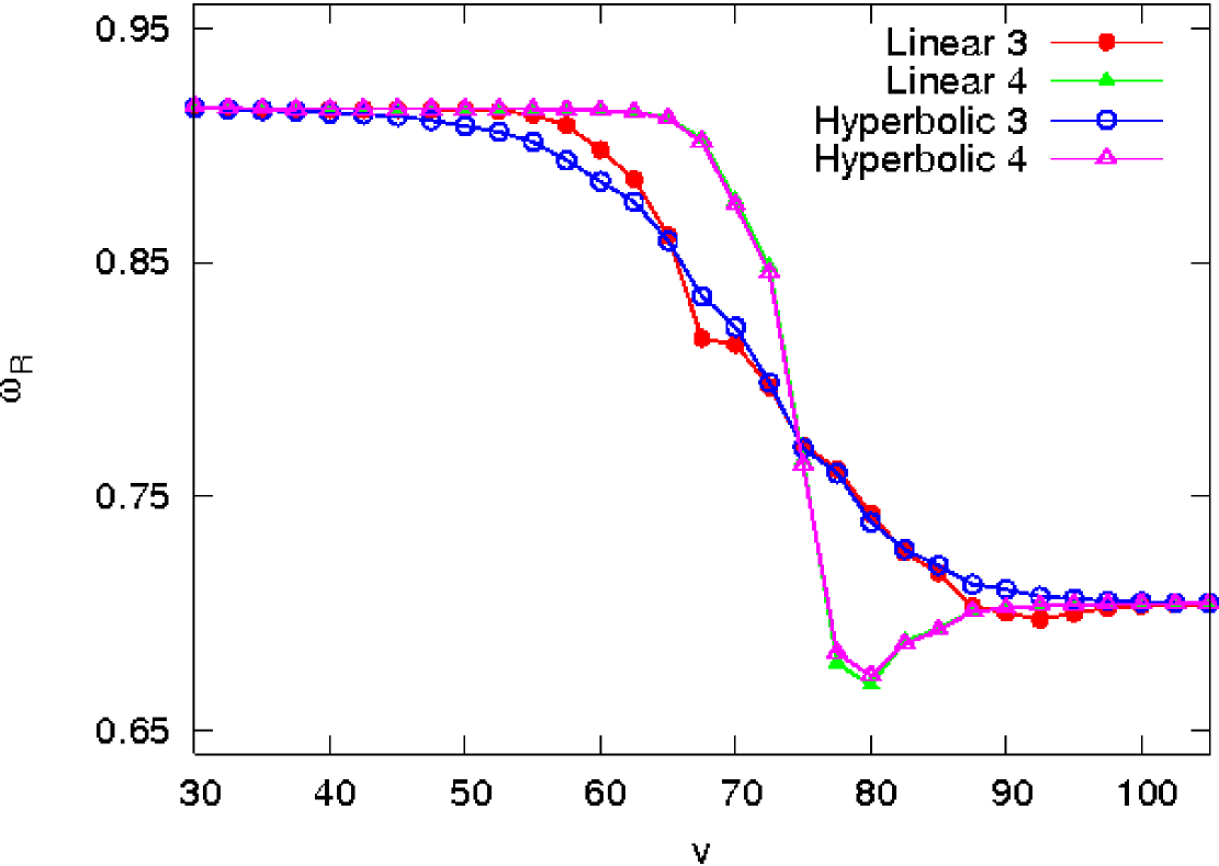
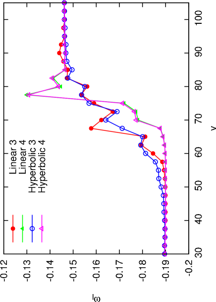
Figure 4: The real ($\omega_{\rm R}$) and imaginary ($\omega_{\rm I}$) part of the frequency for electromagnetic perturbations with $\ell=2$ as function of $v$ for increasing linear and hyperbolic mass functions. For all the cases, $m_{1}=0.5$ and $m_{2}=0.65$. Linear 3: $v_{1}=60$, $v_{2}=90$. Linear 4: $v_{1}=74.5$, $v_{2}=75.5$. Hyperbolic 3: $v_{1}=75$, $\rho=0.08$. Hyperbolic 4: $v_{1}=75$, $\rho=0.8$.

In fact, since the increasing mass functions considered here can be obtained from the decreasing ones by a time-reversal $m(v)\rightarrow m(-v)$, the underlying causal structures are equivalentGS , and the corresponding QNM are also related. Under a time-reversal, the graph of $\omega_{\rm R}$ (and of $\omega_{\rm I}$) must be reflected on a horizontal axis.

We could infer from our numerical simulations the situation corresponding to the onset of the QNM non-stationary inertial behavior. The deviation from the stationary regime is measured by the second derivative of the mass function $m^{\prime\prime}(v)$. Heuristically, one should expect the appearing of non-stationary behavior when $|1/m^{\prime\prime}|$ is smaller than a certain characteristic time of the system, what should prevent the system to relax into an adiabatic regime. There are two characteristic times associated to the QNM of black holes: the oscillation period $2\pi/\omega_{\rm R}$ and the damping time $|1/\omega_{\rm I}|$. The onset of the inertial behavior is associated to the second one. We verify appreciable deviations from the stationary regime whenever $|m^{\prime\prime}(v)|$ is of the same order (or larger) than $|\omega_{\rm I}|$. For instance, for Hyperbolic 2 and Hyperbolic 4 data set (corresponding to the inertial behavior depicted in Figs. 3 and 4) we have $|m^{\prime\prime}_{\rm max}/\omega_{\rm I}^{\rm final}|\approx 25\%$, while for Hyperbolic 1 and Hyperbolic 3 (the stationary behavior) such ratio is 100 times smaller. Estimating the magnitude of the inertial effect from our numerical simulations without an approximated analytical model seems to be much harder. Again heuristically, one expects that the magnitude of the effect be proportional to $|m^{\prime\prime}|\tau$, where $\tau$ is the time interval along which $|m^{\prime\prime}|\gtrapprox|\omega_{\rm I}|$. We could check that the relative variations in frequencies during the inertial behavior for the smooth case are always limited by the ratio $|m^{\prime\prime}/\omega_{\rm I}|$. Further analytical work is certainly necessary to enlighten this point. We finish by noticing that for the $C^{0}$ linear case, $|m^{\prime\prime}_{\rm max}|$ is always large, increasing indeed with $1/\Delta v$, and hence non-stationary inertial behavior is reported in all simulations using $C^{0}$ linear data set. Since $\tau$ is very small in such cases (of the same order of $\Delta v$), the magnitude of the inertial effects are also typically small.

IV Final remarks

All situations we considered in the present work involve mass functions corresponding to an initial black hole with mass $m_{1}$ undergoing some accretion/losing mass process and ending with a mass $m_{2}$. Such an “asymptotic Schwarzschild” choice assures us that the spacetime has the usual black hole causal structure for $v\rightarrow\pm\infty$ and, consequently, that QNM can be defined in the usual way and that the corresponding frequencies can be properly compared. For all the cases considered, the inertial transients dissipate away and $\omega(v)$ tends to follow the track of $m^{-1}(v)$ rather quickly, rendering the robustness of the numerical QNM analysis. The integration in double-null coordinates has turned out to be much more efficient than the integration in radiation coordinatesCheng-04 , allowing us to reach the precision necessary to unveil the reported non-stationary behavior with quite modest computational resources. Despite the radiation coordinates are known to be defective at the horizonradhorizon , we believe that numerical analysis as those one presented in Cheng-04 are still confident since the QNM analysis is always concerned to the exterior region of the black hole. However, as confirmed by the present calculations, algorithms based on the characteristic integration are typically by far more efficient.

An interesting extension of this work would be analysis of the highly damped QNM (overtones, $n>0$). Since for such overtones the ratio $|\omega_{\rm I}/\omega_{\rm R}|$ is always larger than for the $n=0$ QNM considered here, including, for sufficient large $n$, cases for which $|\omega_{\rm I}/\omega_{\rm R}|>1$, it would be interesting to check if the non-stationary inertial behavior could somehow be attenuated for $n>0$. We notice that the numerical analysis presented here cannot be extended directly to the $n>0$ case since one cannot identify the $n>0$ frequencies with sufficient accuracy. We believe this could be attained, in principle, by means of the WKB approximation.

Although the typical astrophysical situations of mass accretion for black holes will hardly keep spherical symmetry intact during intermediate stages, our results can be used as a first approximation for the scattering by this sources since, as it is well known, after the transient phases, the system should accommodate itself in a stationary spherical symmetric configuration. One must, however, keep in mind that non-stationary inertial behavior in the QNM frequencies is expected to take place whenever $|m^{\prime\prime}|\gtrapprox|\omega_{\rm I}|$, rendering the analysis of the rapid variating situations a subtler task.

The evaporation by Hawking radiation could indeed be considered as a physically genuine process where the black hole mass decreases and spherical symmetry is maintained. Our approach can be applied for this case, with some crucial remarks about the causal structure of the spacetime left behind after the evaporationACS .

We finish by noticing, as it is well known, that the damped oscillations correspond to an intermediate phase in the wave scattering by asymptotic flat black holes. The very last final phase corresponds, indeed, to a power law decay. In the problems considered here, the power law tail typically appears for large values of $v$ for which the QNM already settled down in the stationary phase, with no trace from the transients. We do not detect, in this case, any influence of the time-dependence of the potential in these tails. There is no contradiction with the results reported in Hod-02 . This is a consequence of our choice of “asymptotic Schwarzschild” mass functions, for which the corresponding potential has no resemblance with those ones considered in Hod-02 .

- (1) H.P. Nollert, Class. Quantum Grav. 16, R159 (1999).
- (2) K.D. Kokkotas and B.G. Schmidt, Living Rev. Rel. 2, 2 (1999), [arXiv:gr-qc/9909058].
- (3) E. Berti, V. Cardoso and C. M. Will, Phys. Rev. D73, 064030 (2006), [arXiv:gr-qc/0512160].
- (4) P.R. Brady, C.M. Chambers, W. Krivan, and P. Laguna, Phys. Rev. D55, 7538(1997), [arXiv:gr-qc/9611056]; P.R. Brady, C.M. Chambers, W.G. Laarakkers and E. Poisson, Phys. Rev. D60, 064003 (1999), [arXiv:gr-qc/9902010].
- (5) C. Molina, D. Giugno E. Abdalla and A. Saa, Phys. Rev. D69, 104013 (2004), [arXiv:gr-qc/0309079].
- (6) D.P. Du, B. Wang and R.K. Su, Phys. Rev. D70, 064024 (2004), [arXiv:hep-th/0404047]; E. Abdalla, B. Wang, A. Lima-Santos and W.G. Qiu, Phys. Lett. 538B, 435 (2000), [arXiv:hep-th/0204030]; E. Abdalla, K.H.C. Castello-Branco and A. Lima-Santos, Phys. Rev. D66, 104018 (2002), [arXiv:hep-th/0208065].
- (7) S. Hod, Phys. Rev. D66, 024001 (2002), [arXiv:gr-qc/0201017].
- (8) L.H. Xue, Z.X. Shen, B. Wang and R.K. Su, Mod. Phys. Lett. A19, 239 (2004), [arXiv:gr-qc/0304109].
- (9) C.G. Shao, B. Wang, E. Abdalla, and R.K. Su, Phys. Rev. D71, 044003 (2005), [arXiv:gr-qc/0410025].
- (10) J.S.F. Chan and R.B. Mann, Phys. Rev. D55, 7546 (1997), [arXiv:gr-qc/9612026]; Phys. Rev. D59, 064025 (1999).
- (11) V. Cardoso and J.P.S. Lemos, Phys. Rev. D63, 124015 (2001), [arXiv:gr-qc/0101052].
- (12) G.T. Horowitz and V.E. Hubeny, Phys. Rev. D62, 024027 (2000), [arXiv:hep-th/9909056].
- (13) B. Wang, C.Y. Lin and E. Abdalla, Phys. Lett. 481B, 79 (2000), [arXiv:hep-th/0003295].
- (14) B. Wang, C. Molina and E. Abdalla, Phys. Rev. D63, 084001 (2001), [arXiv:hep-th/0005143].
- (15) V. Cardoso and J.P.S. Lemos, Phys. Rev. D64, 084017 (2001), [arXiv:gr-qc/0105103]; Class. Quantum. Grav. 18, 5257 (2001), [arXiv:gr-qc/0107098].
- (16) E. Berti and K.D. Kokkotas, Phys. Rev. D67, 064020 (2003), [arXiv:gr-qc/0301052].
- (17) R.A. Konoplya, Phys. Rev. D66, 044009 (2002), [arXiv:hep-th/0205142].
- (18) D. Birmingham, I. Sachs, S.N. Solodukhin, Phys. Rev. Lett. 88, 151301 (2002), [arXiv:hep-th/0112055]; D. Birmingham, Phys. Rev. D64, 064024 (2001), [arXiv:hep-th/0101194].
- (19) J.M. Zhu, B. Wang and E. Abdalla, Phys. Rev. D63, 124004 (2001), [arXiv:hep-th/0101133]; B. Wang, E. Abdalla and R.B. Mann, Phys. Rev. D65, 084006 (2002), [arXiv:hep-th/0107243]; B. Wang, C.Y. Lin and C. Molina, Phys. Rev. D70, 064025 (2004), [arXiv:hep-th/0407024].
- (20) S. Musiri and G. Siopsis, Phys. Lett. 576B, 309 (2003), [arXiv:hep-th/0308196]; R. Aros, C. Martinez, R. Troncoso and J. Zanelli, Phys. Rev. D67, 044014 (2003), [arXiv:hep-th/0211024]; A. Nunez and A.O. Starinets, Phys. Rev. D67, 124013 (2003), [arXiv:hep-th/0302026]; E. Winstanley, Phys. Rev. D64, 104010 (2001), [arXiv:gr-qc/0106032].
- (21) V. Cardoso and J.P.S. Lemos, Phys. Rev. D67, 084020 (2003), [arXiv:gr-qc/0301078].
- (22) V. Cardoso, R. Konoplya and and J.P.S. Lemos, Phys. Rev. D68, 044024 (2003), [arXiv:gr-qc/0305037].
- (23) B. Waugh and K. Lake, Phys. Rev. D34, 2978 (1986).
- (24) F. Girotto and A. Saa, Phys. Rev. D70, 084014 (2004), [arXiv:gr-qc/0406067].
- (25) Y. Zlochower, R. Gomez, S. Husa, L. Lehner and J. Winicour, Phys. Rev. D68, 084014 (2003), [arXiv:gr-qc/0306098].
- (26) R. Lindquist, R. Schwartz, and C. Misner, Phys. Rev. 137, B1364 (1965).
- (27) E. Abdalla, C. B. M. H. Chirenti, and A. Saa, to appear.