Spectroscopy of Cosmic topology

Abstract

Einstein’s theory of gravitation that governs the geometry of space-time, coupled with spectacular advance in cosmological observations, promises to deliver a ‘standard model’ of cosmology in the near future. However, local geometry of space constrains, but does not dictate the topology of the cosmos. hence, Cosmic topology has remained an enigmatic aspect of the ‘standard model’ of cosmology. Recent advance in the quantity and quality of observations has brought this issue within the realm of observational query. The breakdown of statistical homogeneity and isotropy of cosmic perturbations is a generic consequence of non trivial cosmic topology arising from to the imposed ‘crystallographic’ periodicity on the eigenstates of the Laplacian. The sky maps of Cosmic Microwave Background (CMB) anisotropy and polarization most promising observations that would carry signatures of a violation of statistical isotropy and homogeneity. Hence, a measurable spectroscopy of cosmic topology is made possible using the Bipolar power spectrum (BiPS) of the temperature and polarization that quantifies violation of statistical isotropy.

Inter-University Centre for Astronomy and Astrophysics,
Post Bag 4, Ganeshkhind, Pune 411007, India
E-mail:tarun@iucaa.ernet.in

I Introduction

I feel honored to be invited to contribute to this volume honoring the memory of Professor Amal Kumar Raychaudhuri (fondly known as AKR) – a great scientist and teacher. The Raychaudhuri equations describing the evolution of anisotropic universe models are the footprints of homegrown Indian science in the field of cosmology. Though the background universe is observationally consistent with homogeneous and isotropic Friedmann models, the Raychaudhuri equations appears in the evolution of inhomogeneities that led to the formation of large scale structures in the universe. It is fair to say much of the recent progress in cosmology has come from the interplay between refinement of the theories of structure formation and the improvement of the observations. Hence, the Raychaudhuri equations have remained as relevant and ingrained in contemporary cosmology as when first put forward by AKR. This article describing our ongoing research determine the topology of the universe from the exquisite measurements of anisotropy in the Cosmic Microwave background is a humble tribute to the doyen of Indian science.

The realization that a universe with the same local geometry has many different choices of global topology has been a theoretical curiosity as old as modern cosmology. De Sitter was quick to point out that the first modern model of the cosmos, Einstein’s closed ($S^{3}$, spherical geometry and static) universe model, could equally well correspond to the multiply connected ‘Elliptical’ universe where antipodal point of $S^{3}$ are topologically identified ($S^{3}/Z_{2}$). Fig. 1 depicts the prevalent modern view within the concept of inflation, that this relatively smooth ‘Hubble volume’ that we observe is perhaps a tiny patch of an extremely inhomogeneous and complex spatial manifold. The complexity could involve non-trivial topology (multiple connectivity) on these ultra-large scales. Given the observational support for a homogeneous Hubble volume around us, the diverse possibility of global structure reduces to the tractable study limited to spaces of uniform curvature (locally homogeneous and isotropic FLRW models) but with non-trivial cosmic topology. For example, in Fig. 1, observers in the ‘handle’ regions would perceive an open (hyperbolic geometry ) universe, and those in the ‘bulb’ region observe a closed (spherical geometry) universe. Although, in a generic manifold, sectors with exact Euclidean geometry are rare, an epoch of inflation in the early universe inflate any region to a nearly flat, Euclidean geometry.

The motivation for non-trivial topology and the quest to determine size and the shape of our universe has a rich and diverse history in modern cosmology ell71 ; sok_shv74 ; got80 ; lac_lum95 ; stark98 . Spatially compact universe models have both deep theoretical and philosophical appeal – eg., the quantum creation of finite sized universe from vacuum is a theoretical motivation linde , and a philosophical abhorrence of any ‘infinity’ in nature would argue against an infinite sized universe lev02 . A compact universe, with the exception of the three sphere, $S^{3}$ implies a multiply connected universe (i.e., nontrivial cosmic topology).

The photons of the cosmic microwave background(CMB) propagate freely over distances comparable to the cosmic horizon. The CMB anisotropy and its polarization are the most promising observational probes of the global spatial structure of the universe on length scales near to and even somewhat beyond the ‘horizon’ scale ($\sim cH_{0}^{-1}$). A generic consequence   of cosmic topology is the breaking of statistical isotropy in characteristic patterns determined by the photon geodesic structure of the manifold bps98 . The increasingly exquisite measurements of CMB anisotropy have brought cosmic topology from the realm of theoretical possibility to within the grasp of observations and has received considerable attention over the past few years staro ; stark98 ; levin98 ; bps98 ; bps00a ; bps00b ; angelwmap ; coles-graca . CMB polarization not only augments the CMB temperature anisotropy observations but is expected to allow a more incisive study of cosmic topology since it arises only at the surface of last scattering (SLS). The recent full sky measurements of CMB polarization maps by WMAP has opened the door to this new arena pag06 .

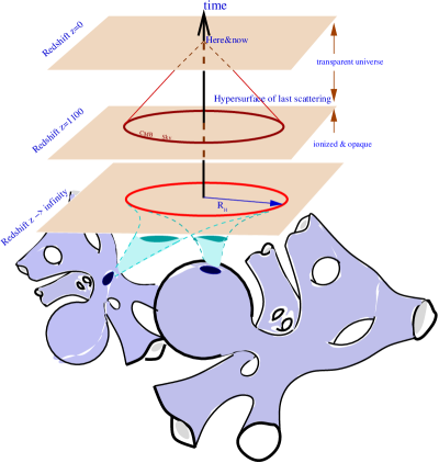
Figure 1: A cartoon depicting a prevalent view within the inflationary paradigm. The observable universe corresponds to a small patch of a very complicated manifold that has been blown to cosmological scales during an inflationary epoch. Ultra-large scale structure could be observable if the the size of this patch is not much smaller that the scales of inhomogeneity and non-trivial topology.

Any multiply-connected space is equivalent to a simply connected space (universal cover) that is tiled by Dirichlet domains (DD) under a free acting subgroup, $\Gamma$ of the isotropy group, $G^{u}$ of universal cover. Hence, even the most complicated cosmic topology reduces to a study of standard FLRW models with periodic boundary conditions on the appropriate DD. A simple example being the 3-torus $T^{3}$, that is equivalent to the study of a universe in a box with periodic boundary conditions – a routine approximation in numerical simulations of large scale structure in the universe. More formally, the $T^{3}$ is obtained by tiling 3-D Euclidean space under the isometry subgroup of discrete translations in three directions. In cosmology, the Dirichlet domain constructed around the observer represents the universe as ‘seen’ by the observer. The SI breakdown is apparent in the principal axes present in the shape of the DD constructed with the observer located at the base-point us_prl . Equivalently, the fields defining perturbations are built of the subset of eigenstates of Laplacian that invariant under $\Gamma$. The correlations of CMB fluctuations in the sky would have patterns that are no longer invariant under rotations.

In a cosmological model with trivial topology, the CMB anisotropy signal is expected to be statistically isotropic, i.e., statistical expectation values of the temperature fluctuations $\Delta T(\hat{q})$ are preserved under rotations of the sky. In particular, the angular correlation function $C(\hat{q},\,\hat{q}^{\prime})\equiv\langle\Delta T(\hat{q})\Delta T(\hat{q}^{\prime})\rangle$ is rotationally invariant for Gaussian fields, i.e., $C(\hat{q},\,\hat{q}^{\prime})\equiv C(\hat{q}\cdot\hat{q}^{\prime})$. In spherical harmonic space, where $\Delta T(\hat{q})=\sum_{lm}a_{lm}Y_{lm}(\hat{q})$, the condition of statistical isotropy (SI) translates to a diagonal $\langle a_{lm}a^{*}_{l^{\prime}m^{\prime}}\rangle=C_{l}\delta_{ll^{\prime}}\delta_{mm^{\prime}}$ where $C_{l}$, the widely used angular power spectrum of CMB anisotropy. The correlation patterns in the CMB anisotropy that lead to violation of SI implies that imply $\langle\hat{a}_{lm}\hat{a}^{*}_{lm}\rangle$ has off-diagonal elements. Figure 2 taken from  bps00b shows the off-diagonal elements in the CMB correlation for two compact universe models.

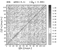
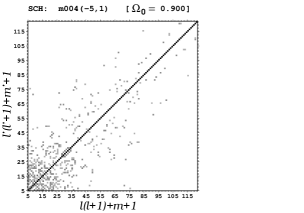
Figure 2: The figure taken from bps00b illustrates the non-diagonal nature of the expectation values of $a_{\ell m}$ pair products when the CMB anisotropy violates SI in two model compact universe. The radical violation in the model on the left corresponds to a small compact universe where CMB photons have traversed across multiple times. The model on the left with mild violation of SI corresponds to a universe of size comparable to the observable horizon. For more details, see bps00b

The observed CMB sky $\widetilde{\Delta T}(\hat{n})$ is a single realization of the underlying correlation, hence the detection of SI violation or correlation patterns pose a great observational challenge . For statistically isotropic CMB sky, the correlation function

$$C(\hat{n}_{1},\hat{n}_{2})\equiv C(\hat{n}_{1}\cdot\hat{n}_{2})=\frac{1}{8\pi^{2}}\int d{\mathcal{R}}\,\,C({\mathcal{R}}\hat{n}_{1},\,{\mathcal{R}}\hat{n}_{2}),$$ (1)

where ${\mathcal{R}}\hat{n}$ denotes the direction obtained under the action of a rotation ${\mathcal{R}}$ on $\hat{n}$, and $d{\mathcal{R}}$ is a volume element of the three-dimensional rotation group. The invariance of the underlying statistics under rotation allows the estimation of $C(\hat{n}_{1}\cdot\hat{n}_{2})$ using the average of the temperature product $\widetilde{\Delta T}(\hat{n})\widetilde{\Delta T}(\hat{n}^{\prime})$ between all pairs of pixels with the angular separation $\theta$. In the absence of statistical isotropy, $C(\hat{n},\hat{n}^{\prime})$ is estimated by a single product $\widetilde{\Delta T}(\hat{n})\widetilde{\Delta T}(\hat{n}^{\prime})$ and, hence, is poorly determined from a single realization.

Although it is not possible to estimate each element of the full correlation function $C(\hat{n},\hat{n}^{\prime})$, some measures of statistical anisotropy of the CMB map can be estimated through suitably weighted angular averages of $\widetilde{\Delta T}(\hat{n})\widetilde{\Delta T}(\hat{n}^{\prime})$. The angular averaging procedure should be such that the measure involves averaging over sufficient number of independent ‘measurements’, but should ensure that the averaging does not erase all the signature of statistical anisotropy. Recently, we proposed the Bipolar Power spectrum (BiPS) $\kappa_{\ell}$ ($\ell=1,2,3,\ldots$) of the CMB map as a statistical tool of detecting and measuring departure from SI us_apjl . The BiPS is formally defined as

$$\kappa^{\ell}\,=\,(2l+1)^{2}\int d\Omega_{n_{1}}\int d\Omega_{n_{2}}\,[\frac{1}{8\pi^{2}}\int d{\mathcal{R}}\chi^{\ell}({\mathcal{R}})\,C({\mathcal{R}}\hat{n}_{1},\,{\mathcal{R}}\hat{n}_{2})]^{2}.$$ (2)

In the above expression, $C({\mathcal{R}}\hat{n}_{1},\,{\mathcal{R}}\hat{n}_{2})$ is the two point correlation at ${\mathcal{R}}\hat{n}_{1}\,$ and ${\mathcal{R}}\hat{n}_{2}$ which are the coordinates of the two pixels $\hat{n}_{1}\,$ and $\hat{n}_{2}$ after rotating the coordinate system by element ${\mathcal{R}}$ of the rotation group.

$\chi^{\ell}({\mathcal{R}})$ is the trace of the finite rotation matrix in the $\ell M$-representation

$$\chi^{\ell}({\mathcal{R}})\,=\,\sum_{M=-\ell}^{\ell}D_{MM}^{\ell}({\mathcal{R}}),$$ (3)

which is called the characteristic function, or the character of the irreducible representation of rank $\ell$. It is invariant under rotations of the coordinate systems. in eq.(2) $d{\mathcal{R}}$ is the volume element of the three-dimensional rotation group. For a statistically isotropic model $C(\hat{n}_{1},\,\hat{n}_{2})$ is invariant under rotation, and therefore $C({\mathcal{R}}\hat{n}_{1},\,{\mathcal{R}}\hat{n}_{2})\,=\,C(\hat{n}_{1},\,\hat{n}_{2})$ and the orthonormality of $\chi^{\ell}(\omega)$, we will recover the condition for SI,

$$\kappa^{\ell}\,=\,\kappa^{0}\delta_{\ell 0}.$$ (4)

The Bipolar power spectrum gets it name from its interpretation in the harmonic space. The two point correlation of CMB anisotropies, $C(\hat{n}_{1},\,\hat{n}_{2})$, is a two point function on $S^{2}\times S^{2}$, and hence can be expanded as

$$C(\hat{n}_{1},\,\hat{n}_{2})\,=\,\sum_{l_{1},l_{2},L,M}A_{l_{1}l_{2}}^{\ell M}\,\,\{Y_{l_{1}}(\hat{n}_{1})\otimes Y_{l_{2}}(\hat{n}_{2})\}_{\ell M},$$ (5)

where $A_{l_{1}l_{2}}^{\ell M}$ are coefficients of the expansion (here after BipoSH coefficients) and $\{Y_{l_{1}}(\hat{n}_{1})\otimes Y_{l_{2}}(\hat{n}_{2})\}_{\ell M}$ are the Bipolar spherical harmonics which transform as a spherical harmonic with $\ell,\,M$ with respect to rotations Var given by

$$\{Y_{l_{1}}(\hat{n}_{1})\otimes Y_{l_{2}}(\hat{n}_{2})\}_{\ell M}\,=\,\sum_{m_{1}m_{2}}{\mathcal{C}}_{l_{1}m_{1}l_{2}m_{2}}^{\ell M}Y_{l_{1}m_{1}}(\hat{n}_{2})Y_{l_{2}m_{2}}(\hat{n}_{2}),$$ (6)

in which ${\mathcal{C}}_{l_{1}m_{1}l_{2}m_{2}}^{\ell M}$ are Clebsch-Gordan coefficients. We can inverse-transform $C(\hat{n}_{1},\,\hat{n}_{2})$ to get the $A_{l_{1}l_{2}}^{\ell M}$ by multiplying both sides of eq.(5) by $\{Y_{l^{\prime}_{1}}(\hat{n}_{1})\otimes Y_{l^{\prime}_{2}}(\hat{n}_{2})\}_{\ell^{\prime}M^{\prime}}^{*}$ and integrating over all angles, then the orthonormality of bipolar harmonics implies that

$$A_{l_{1}l_{2}}^{\ell M}\,=\,\int d\Omega_{\hat{n}_{1}}\int d\Omega_{\hat{n}_{2}}\,C(\hat{n}_{1},\,\hat{n}_{2})\,\{Y_{l_{1}}(\hat{n}_{1})\otimes Y_{l_{2}}(\hat{n}_{2})\}_{\ell M}^{*}.$$ (7)

The above expression and the fact that $C(\hat{n}_{1},\,\hat{n}_{2})$ is symmetric under the exchange of $\hat{n}_{1}$ and $\hat{n}_{2}$ lead to the following symmetries of $A_{l_{1}l_{2}}^{\ell M}$

$$A_{l_{2}l_{1}}^{\ell M}\, = \,(-1)^{(l_{1}+l_{2}-L)}A_{l_{1}l_{2}}^{\ell M},$$ (8)

$$A_{ll}^{\ell M}\, = \,A_{ll}^{\ell M}\,\,\delta_{\ell,2k},\,\,\,\,\,\,\,\,\,\,\,\,\,\,\,\,\,\,\,\,\,k=0,\,1,\,2,\,\cdots.$$

The Bipolar Spherical Harmonic (BipoSH) coefficients, $A_{l_{1}l_{2}}^{\ell M}$, are linear combinations of off-diagonal elements of the harmonic space covariance matrix,

$$A^{\ell M}_{l_{1}l_{2}}\,=\,\sum_{m_{1}m_{2}}\langle a_{l_{1}m_{1}}a^{*}_{l_{2}m_{2}}\rangle(-1)^{m_{2}}C^{\ell M}_{l_{1}m_{1}l_{2}-m_{2}}.$$ (9)

This means that $A^{\ell M}_{l_{1}l_{2}}$ completely represent the information of the covariance matrix in harmonic space $\langle a_{l_{1}m_{1}}a^{*}_{l_{2}m_{2}}\rangle$. When SI holds, the harmonic space covariance matrix is diagonal and hence

$$A_{ll^{\prime}}^{\ell M}\, = \,(-1)^{l}C_{l}(2l+1)^{1/2}\,\delta_{ll^{\prime}}\,\delta_{\ell 0}\,\delta_{M0},$$ (10)

$$A^{00}_{l_{1}l_{2}}\, = \,(-1)^{l_{1}}\sqrt{2l_{1}+1}\,C_{l_{1}}\,\delta_{l_{1}l_{2}}.$$

BipoSH expansion is the most general representation of the two point correlation functions of CMB anisotropy. The well known angular power spectrum, $C_{l}$ is a subspace of BipoSH coefficients corresponding to the $A_{ll}^{00}$ that represent the statistically isotropic part of a general correlation function. When SI holds, $A_{ll}^{00}$ or equivalently $C_{l}$ have all the information of the field. But when SI breaks down, $A_{ll}^{00}$ are not adequate for describing the field, and one needs to take the other terms into account. The Bipolar power spectrum (BiPS) is defined as a rotationally invariant contraction of the BipoSH coefficients

$$\kappa_{\ell}\,=\,\sum_{l,l^{\prime},M}|A_{ll^{\prime}}^{\ell M}|^{2}\geq 0.$$ (11)

This definition is identical to the real space expression in eq. (2). More importantly, BiPS is measurable from a single CMB map since averages over many independent modes and reduces the cosmic variance  us_apjl . The BiPS of the CMB anisotropy maps measured by WMAP has been computedus_apjl2 . Preliminary BiPS results on the CMB polarization maps from the three year of WMAP data have also emerged in past few months bas06 ; uci_si06 .

The BiPS is sensitive to structures and patterns in the underlying total two-point correlation function us_apjl ; us_pascos . The BiPS is particularly sensitive to real space correlation patterns (preferred directions, etc.) on characteristic angular scales. In harmonic space, the BiPS at multipole $\ell$ sums power in off-diagonal elements of the covariance matrix, $\langle a_{lm}a_{l^{\prime}m^{\prime}}\rangle$, in the same way that the ‘angular momentum’ addition of states $lm$, $l^{\prime}m^{\prime}$ have non-zero overlap with a state with angular momentum $|l-l^{\prime}|<\ell<l+l^{\prime}$. Signatures, like $a_{lm}$ and $a_{l+nm}$ being correlated over a significant range $l$ are ideal targets for BiPS. These are typical of SI violation due to cosmic topology and the predicted BiPS in these models have a strong spectral signature in the bipolar multipole $\ell$ space us_prl . The orientation independence of BiPS is an advantage since one can obtain constraints on cosmic topology that do not depend on the unknown (but specific) orientation of the pattern (e.g., preferred directions of DD relative to the sky).

Spaces of constant curvature have been completely classified wol94vin93 ; thur79 . For Euclidean geometry, there are known to be six possible topologies that lead to orientable spaces. The simple flat torus, ${\cal M}=T^{3}$, is obtained by identifying the universal cover ${\cal M}^{u}={\cal E}^{3}$ under a discrete group of translations along three non-degenerate axes, ${\mathbf{s}_{1},\mathbf{s}_{2},\mathbf{s}_{3}}$: ${\mathbf{s}_{i}}\to{\mathbf{s}_{i}}+{\mathbf{n}}L_{i}$, where $L_{i}$ is the identification length of the torus along $s_{i}$ and ${\bf n}$ is a vector with integer components. In the most general form, the fundamental domain (FD) is a parallelepiped defined by three sides $L_{i}$ and the three angles $\alpha_{i}$ between the axes (‘squeezed torus’). If ${\mathbf{s}_{i}}$ are orthogonal then one gets cuboid FD, which for equal $L_{i}$ reduces to the cubic torus. The cuboid and squeezed spaces which can be obtained by a linear coordinate transformation ${\cal L}$ on cubic torus can have distinctly different global symmetry .

Study of the BiPS signature of cosmic topology has already been undertaken and ongoing us_prl ; us_big ; us_dodeca . The correlation function $C({\hat{q},\hat{q}^{\prime}})$ for CMB anisotropy in a multiply-connected universe such as the torus space can be computed using the regularized method of imagesbps00a . Fig. 3 plots the predicted $\kappa_{\ell}$ spectrum for a number of cubic, cuboid and squeezed torus spaces us_prl . Similar results for Poincaré Dodecahedron show a characteristic BiPS with a dominant peak at $\kappa_{6}$ over a range of value of curvature radius (including integrated Sachs-Wolfe effect). This relates to the angular separation of the directions to faces of the extremely symmetric DD of Poincaré dodecahedral space. Fig. 3 shows that $\kappa_{\ell}$ is zero for odd $\ell$. This is intimately related to the symmetries of the Dirichlet domain, which in turn is dictated by the properties of the subgroup of isometries $\Gamma$. The BiPS is zero at odd bipolar multipoles if DD has $2n$-fold symmetry about an axis and reflection symmetry in an orthogonal plane. It can be proved that all Euclidean and all spherical spaces generated by single action $\Gamma$ satisfy this condition. Remarkably enough, compact hyperbolic spaces do not satisfy these condition, and are generically expected to have non-zero BiPS at odd value bipolar multipoles $\ell$ him06 . This provides a measurable classification of cosmic topology based on CMB anisotropy and polarization, i.e., a spectroscopy of cosmic topology.

A simple working example is the BiPS signature of a non-trivial topology can be given for a $T^{3}$ universe, where the correlation function is given by

$$C({\hat{q},\hat{q}^{\prime}})=L^{-3}\sum_{{\bf n}}P_{\Phi}(k_{\bf n})\,\,{\mathrm{e}}^{-i\pi(\epsilon_{\hat{q}}{\bf n}\cdot{\hat{q}}-\epsilon_{\hat{q}^{\prime}}{\bf n}\cdot{\hat{q}}^{\prime})},$$ (12)

in which, ${\bf n}$ is 3-tuple of integers (in order to avoid confusion, we use $\hat{q}$ to represent the direction instead of $\hat{n}$), the small parameter $\epsilon_{\hat{q}}\leq 1$ is the physical distance to the SLS along $\hat{q}$ in units of $L/2$ (more generally, $\bar{L}/2$ where $\bar{L}=(L_{1}L_{2}L_{3})^{1/3}$) and $L$ is the size of the Dirichlet domain (DD). When $\epsilon$ is a small constant, the leading order terms in the correlation function eq. (12) can be readily obtained in power series expansion in powers of $\epsilon$. For the lowest wave numbers $|{\mathbf{n}}|^{2}=1$ in a cuboid torus us_prl

$$C({\hat{q},\hat{q}^{\prime}}) \approx 2\sum_{i}P_{\Phi}({2\pi}/{L_{i}})\cos(\pi\epsilon\beta_{i}\Delta q_{i})$$

$$\approx C_{0}\left[1-\epsilon^{2}\,|{\mathbf{\Delta}q}|^{2}+3\,\epsilon^{4}\,\sum_{i=1}^{3}(\Delta q_{i})^{4}\right],$$

where $\Delta q_{i}$ are the components of ${\mathbf{\Delta}q}=\hat{q}-\hat{q}^{\prime}$ along the three axes of the torus and $\beta_{i}=\bar{L}/L_{i}$. From this, the non-zero $\kappa_{\ell}$ can be analytically computed to be

$$\frac{\kappa_{0}}{C_{0}^{2}}\, = \,\pi^{2}(1-4\epsilon^{2}+\frac{368}{15}\epsilon^{4}-\frac{288}{5}\epsilon^{6}+\frac{20736}{125}\epsilon^{8})$$

$$\frac{\kappa_{4}}{C_{0}^{2}}\, = \,\frac{12288\pi^{2}}{875}\epsilon^{8}\,\,.$$ (14)

$\kappa_{4}$ has the information of the relative size of the Dirichlet domain and one can use it to constrain the topology of the universe.

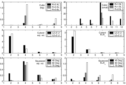
Figure 3: The figure taken from us_prl shows the BiPS $\kappa_{\ell}$ spectra for flat tori models . The top row panels are for cubic tori spaces. The left panel shows spaces of volume, $V_{\cal M}$, larger than the volume $V_{*}$ contained in the sphere of last scattering (SLS) with $V_{\cal M}/V_{*}=3.7,1.9,1.1$, respectively. The right panel shows small spaces with $V_{\cal M}/V_{*}=0.24,0.07,0.03$, respectively. Note that $\kappa_{2}=0$ for cubic tori. The middle panels consider cuboid tori with $1:5$ and $1:2$ ratio of identification lengths. The bottom panels show $\kappa_{\ell}$ for equal-sided squeezed tori with $\alpha=45^{\circ},60^{\circ}$ and $75^{\circ}$. In the middle and bottom rows, the right panels show the case when radius of SLS, $R_{*}=R_{<}$ the in-radius of the space. Here, the SLS just touches its nearest images which is at the threshold where CMB anisotropy is multiply imaged for larger $R_{*}$. The cases in the left panels of lower two rows have $V_{\cal M}/V_{*}=1$ and are at the divide between large and small spaces.

The results of WMAP are a milestone in CMB anisotropy measurements since it combines high angular resolution, high sensitivity, with ‘full’ sky coverage allowed by a space mission. The Wilkinson Microwave Anisotropy Probe (WMAP) observations are consistent with the predictions of the concordance $\Lambda$CDM model with scale-invariant and adiabatic fluctuations which have been generated during the inflationary epoch ben_wmap03 ; hin_wmap06 ; sper_wmap06 . After the first year of WMAP data, the SI of the CMB anisotropy (i.e. rotational invariance of n-point correlations) has attracted considerable attention. Tantalizing evidence of SI breakdown (albeit, in very different guises) that mounted in the WMAP first year sky maps, using a variety of different statistics are expected to persist in the three persist in three year data (see uci_si06 for discussion and references.).

The CMB anisotropy map based on the WMAP data are ideal for testing for statistical isotropy. Preferred directions and statistically anisotropic CMB anisotropy have been discussed in literature earlier fer_mag97 ; bun_scot00 . A number of direct searches for signature of cosmic topology have been proposed and carried out on early CMB data from COBE-DMR. Full Bayesian likelihood comparison to the data of specific cosmic topology models is another approach that has applied to COBE-DMR data bps98 ; bps00a ; bps00b . The generic features of $\kappa_{\ell}$ spectrum are related to the symmetries of correlation pattern. For cosmic topology, $\kappa_{\ell}$ are sensitive to SI violation even when CMB is not multiply imaged. The orientation independence of BiPS is an advantage for constraining patterns (preferred directions) with unspecified orientation in the CMB sky such as that arising due to cosmic topology or, anisotropic cosmology Ghosh et al. (2006). Extension of BiPS analysis to CMB polarization maps has been studied recently bas06 ; uci_si06 adds a new dimension to the spectroscopy of cosmic topology.

In summary, there are strong theoretical and philosophical motivations for a non-trivial cosmic topology. The breakdown of statistical homogeneity and isotropy of cosmic perturbations is a generic feature of non trivial cosmic topology. A promising observational approach is to hunt for SI violation in the CMB anisotropy. The underlying correlation patterns in the CMB anisotropy and polarization in a multiply connected universe is related to the symmetry of the Dirichlet domain. BiPS has the advantage of being independent of the overall orientation of the Dirichlet domain with respect to the sky. The pattern of SI violation of a cosmic topology leads to a measurable, characteristic Bipolar power spectrum related to the principle directions in the Dirichlet domain and symmetries of the two point correlation function. The Bipolar power spectroscopy of cosmic topology presents itself as promising pursuit for current and upcoming measurements of CMB anisotropy and polarization.

The author acknowledges years of very fruitful collaboration with Dick Bond and Dmitry Pogosyan. Amir Hajian devoted most of his doctoral thesis to this effort and the results mentioned here were jointly obtained with him The article also includes recent and ongoing work done with Himan Mukhopadhyay and Soumen Basak.

References

- (1) G. F. R. Ellis, Gen. Rel. Grav. 2, 7 (1971).
- (2) D. D. Sokolov and V. F. Shvartsman (1974) Zh. Eksp. Theor. Fiz. 66, 412 [JETP, 39, 196 (1974)].
- (3) J. R. Gott, Mon. Not. R. Astr. Soc. 193, 153 (1980).
- (4) M. Lachieze-Rey and J. -P. Luminet, Phys. Rep. 25, 136, (1995).
- (5) G. Starkman, Class., Quantum Grav. 15, 2529 (1998).
- (6) A. Linde JCAP 0410, 004, (2004)
- (7) J. Levin, Phys. Rep. 365, 251, (2002).
- (8) T. Souradeep, in ‘The Universe’, eds. Dadhich, N. & Kembhavi, A., (Kluwer 2000).
- (9) J. R. Bond, D. Pogosyan & T. Souradeep, Class. Quant. Grav. 15, 2671 (1998).
- (10) A. de Oliveira-Costa, G. F. Smoot, A. A. Starobinsky, , ApJ 468, 457 (1996)
- (11) J. Levin, E. Scannapieco, J. Silk , Class.Quant.Grav. 15, 2689, (1998).
- (12) J. R. Bond, D. Pogosyan & T. Souradeep, Phys. Rev. D 62,043005 (2000).
- (13) J. R. Bond, D. Pogosyan & T. Souradeep, Phys. Rev. D 62,043006 (2000).
- (14) A. de Oliveira-Costa, M. Tegmark, M. Zaldarriaga, & A. Hamilton, 2004, Phys. Rev.D69, 063516.
- (15) P. Dineen, G. Rocha, P. Coles, Mon.Not.Roy.Astron.Soc. 358, 1285 (2005)
- (16) C. J. Copi, D. Huterer and G. D. Starkman, Phys. Rev. D 70, 043515 (2004)
- (17) L. Page et al., preprint 2006.
- (18) A. Hajian, & T. Souradeep, preprint (astro-ph/0301590).
- (19) A. Hajian and T. Souradeep ApJ Lett. 597, L5 (2003).
- (20) D. A. Varshalovich, A. N.Moskalev, V. K.Khersonskii, Quantum Theory of Angular Momentum (World Scientific, 1988).
- (21) A. Hajian & T. Souradeep & N. Cornish, Astrophys. J. Lett. 618, L63 (2005).
- (22) S. Basak, A. Hajian & T. Souradeep, Phys. Rev. D 74, 021301(R) (2006).
- (23) T. Souradeep, A. Hajian and S. Basak, preprint Proc. of ‘Fundamental Physics With CMB workshop’, UC Irvine, March 23-25, 2006, to be published in New Astronomy Reviews (astro-ph/0607577).
- (24) T. Souradeep, and A. Hajian Pramana, 62, 793, (2004).
- (25) J. A. Wolf, Space of Constant Curvature (5th ed.), (Publish or Perish, Inc., 1994); E. B. Vinberg, Geometry II – Spaces of constant curvature,
- (26) W. P. Thurston, The Geometry of 3-Manifolds,lecture notes, (Princeton University 1979).
- (27) A. Hajian, & T. Souradeep, preprint (astro-ph/0501001)
- (28) A.Hajian, D. Pogosyan, T. Souradeep, C.Contaldi, J. R. Bond, in preparation; Proc. 20th IAP Colloquium on Cosmic Microwave Background physics and observation, 2004.
- (29) H. Mukhopadhyay and T. Souradeep, in preparation.
- (30) C. L. Bennett et al., Astrophys.J.Suppl. 148, 1, (2003).
- (31) G. Hinshaw et al., preprint , (astro-ph/0603451).
- (32) D. Spergel et al., preprint, (astro-ph/0603449).
- (33) P. G. Ferreira & J. Magueijo, Phys. Rev. D56, 4578, (1997).
- (34) E. Bunn & D. Scott, M.N.R.A.S., 313, 331, (2000).
- Ghosh et al. (2006) T. Ghosh, A. Hajian and T. Souradeep,preprint [arXiv:astro-ph/0604279].