The recollapse problem of closed isotropic models in second order gravity theory

Abstract

We study the closed universe recollapse conjecture for positively curved Friedmann-Robertson-Walker (FRW) models in the Jordan frame of the second order gravity theory. We analyse the late time evolution of the model with the methods of the dynamical systems. We find that an initially expanding closed FRW universe, starting close to the Minkowski spacetime, may exhibit oscillatory behaviour.

1 Introduction

Since the discovery that general relativity (GR) can been derived from an action principle, many nonlinear Lagrangians have been used for the construction of a metric theory of gravity. The reasons for considering higher order generalisations of the Einstein-Hilbert action are multiple. Firstly, there is no a priori physical reason to restrict the gravitational Lagrangian to a linear function of the scalar curvature $R.$ Secondly it is hoped that higher order Lagrangians would create a first approximation to an as yet unknown theory of quantum gravity. Thirdly one expects that, on approach to a spacetime singularity, curvature invariants of all orders ought to play an important dynamical role. Far from the singularity, when higher order corrections become negligible, one should recover general relativity.

An other important motivation for considering generalised theories of gravity is the hope that these theories might exhibit better behaviour near singularities. General relativity leads to singularities in the spacetimes of all known cosmological models with ordinary matter. Higher order curvature corrections in the gravitational action may rectify the problem and lead to cosmological models free from such pathologies, at the cost of diverging from a FRW behavior at late times [1]. There is a resurgence of interest in such theories which naturally arise in string-theoretic considerations (cf. brane models with Gauss-Bonett terms [2]). These theories are considered as alternatives to general relativity in an effort to explain the accelerating expansion of the universe [3] (for a pedagogical review see [4]).

This talk is about the late evolution of a closed FRW universe in vacuum in the context of the quadratic gravity theory. Section 2 is a short exposition of the field equations obtained from a Lagrangian which is a function of the Ricci curvature. The conformal equivalence of these theories with the Einstein equations having a scalar field as a matter source is discussed. In section 3 we investigate the structure of the four-dimensional dynamical system describing the evolution of a closed FRW universe in quadratic gravity. We find that periodic solutions may prevent this universe from recollapse.

2 Jordan versus Einstein frame

We consider higher order gravity theories (HOG) in vacuum derived from Lagrangians of the form

$$L=f\left(R\right)\sqrt{-g},$$ (1)

where $f$ is an arbitrary smooth function and $R$ is the Ricci curvature. By varying $L$ with respect to the metric tensor, we obtain the vacuum fourth-order field equations

$$f^{\prime}\left(R\right)R_{\mu\nu}-\frac{1}{2}f\left(R\right)g_{\mu\nu}-\nabla_{\mu}\nabla_{\nu}f^{\prime}\left(R\right)+g_{\mu\nu}\square f^{\prime}\left(R\right)=0,$$ (2)

where $\square=g^{\mu\nu}\nabla_{\mu}\nabla_{\nu}$ and a prime (^′) denotes differentiation with respect to $R.$ It is well known (see [5]), that under the conformal transformation

$$\widetilde{g}_{\mu\nu}=f^{\prime}\left(R\right)g_{\mu\nu},$$ (3)

the field equations reduce to the Einstein field equations with a scalar field as a matter source, namely

$$\widetilde{G}_{\mu\nu}=T_{\mu\nu}\left(\widetilde{g},\phi\right),$$

where

$$T_{\mu\nu}\left(\widetilde{g},\phi\right)=\partial_{\mu}\phi\partial_{\nu}\phi-\frac{1}{2}\widetilde{g}_{\mu\nu}\left[\left(\partial\phi\right)^{2}-2V\left(\phi\right)\right],$$

and

$$\phi=\sqrt{\frac{3}{2}}\ln f^{\prime}\left(R\right).$$ (4)

Assuming that (4) can be solved for $R$ to obtain a function $R\left(\phi\right),$ the potential of the scalar field is given by

$$V=\frac{1}{2\left(f^{\prime}\right)^{2}}\left(Rf^{\prime}-f\right).$$ (5)

The conformal equivalence between higher order gravity and general relativity is sometimes expressed formally as “HOG = GR + scalar field”. However this “equation” is an oversimplification of the picture. The two frames are mathematically equivalent, but physically they provide different theories. In the Jordan frame, gravity is described entirely by the metric $g_{\mu\nu}.$ In the Einstein frame, the scalar field exhibits a “non-metric” aspect of the gravitational interaction, reflecting the additional degree of freedom due to the higher order of the field equations in the Jordan frame.

If matter fields, collectively denoted by $\Psi,$ are present in the Jordan frame, the corresponding field equations become

$$f^{\prime}R_{\mu\nu}-\frac{1}{2}fg_{\mu\nu}-\nabla_{\mu}\nabla_{\nu}f^{\prime}+g_{\mu\nu}\square f^{\prime}=T_{\mu\nu}\left(g,\Psi\right).$$ (6)

The generalised Bianchi identities imply that

$$\nabla^{\mu}T_{\mu\nu}\left(g,\Psi\right)=0$$

Therefore, free particles move on geodesics in the Jordan frame. We pass to the Einstein frame by conformally transforming (6) to obtain

$$\widetilde{G}_{\mu\nu}=T_{\mu\nu}\left(\widetilde{g},\phi\right)+\widetilde{T}_{\mu\nu}\left(g,\widetilde{g},\Psi\right).$$ (7)

Now the Bianchi identities imply that

$$\widetilde{\nabla}^{\mu}\widetilde{T}_{\mu\nu}\left(g,\widetilde{g},\Psi\right)\neq 0,\ \ \ \ \widetilde{\nabla}^{\mu}T_{\mu\nu}\left(\widetilde{g},\phi\right)\neq 0.$$

Therefore, equations (7) are formally the Einstein equations, but this theory is not physically equivalent to GR. Of course one could firstly conformally transform the vacuum Lagrangian (1) into the Einstein frame to obtain

$$\widetilde{L}=\sqrt{-\widetilde{g}}\left(\widetilde{R}-\widetilde{g}^{\mu\nu}\partial_{\mu}\phi\partial_{\nu}\phi-2V\left(\phi\right)\right),$$

and then add the matter Lagrangian $L_{m}\left(\widetilde{g},\Psi\right)$ with minimal coupling. In that case, the stress-energy tensors of both fields $\phi$ and $\Psi$ are separately conserved,

$$\widetilde{\nabla}^{\mu}T_{\mu\nu}\left(\widetilde{g},\Psi\right)=0,\ \ \ \ \widetilde{\nabla}^{\mu}T_{\mu\nu}\left(\widetilde{g},\phi\right)=0.$$

This discussion raises the question: which is the physical metric? There is no universally acceptable answer to this question in the literature (see [6, 7] for a thorough presentation of different views).

There is another subtle issue, rarely discussed. The conformal transformation (3) preserves the causal structure of the two frames only if $f^{\prime}\left(R\right)$ is non-negative on the whole spacetime. A weaker assumption is that $f^{\prime}$ has the same sign on a connected open subset of the spacetime. However, both assumptions rely on the knowledge of the function $R,$ and this is possible only after the field equations have been solved. In any case, the conformal transformation (3) may fail to be regular at all points of the spacetime.

3 Cosmological considerations

Since it is easier to tackle a problem in the context of general relativity than using the fourth-order equations (2), the conformal equivalence theorem allows certain results valid in general relativity to be transferred in HOG. If a problem can been solved in the Jordan frame it should be interesting to compare this result with the solution of the same problem obtained in the Einstein frame.

We investigate the closed-universe recollapse conjecture for the $f\left(R\right)=R+\beta R^{2}$ theory. This conjecture states roughly that a closed universe cannot expand for ever, provided that the matter content satisfies some energy conditions and has non-negative pressures. For homogeneous and isotropic spacetimes in the Einstein frame this conjecture was found to be true for vacuum models [8] and for models with a perfect fluid with equation of state $p=(\gamma-1)\rho,$ $2/3<\gamma<2$ [9]. More precisely it was shown that, an initially expanding closed FRW universe, starting close to the Minkowski spacetime cannot avoid recollapse. For the $R+\beta R^{2}$ theory in the Einstein frame in vacuum, the state of the system is defined by $\left(a,\dot{a},\phi,\dot{\phi}\right)\in\mathbb{R}^{4}$ and one has a problem of scalar-field cosmology with a potential (cf. equation (5))

$$V\left(\phi\right)=\frac{1}{8\beta}\left(1-e^{-\sqrt{2/3}\,\phi}\right)^{2}.$$

From the general field equations (2) we obtain the trace equation

$$\ddot{R}+3H\dot{R}+\frac{1}{6\beta}R=0,$$

and the $0-0$ equation

$$\dot{R}=\frac{R^{2}}{12H}-RH-\frac{H}{2\beta}-\frac{Rk}{Ha^{2}}-\frac{k}{2\beta Ha^{2}}$$

in vacuum. Setting $x=1/a$ our dynamical system in vacuum is

$$\dot{R} =v,$$

$$\dot{v} =-3Hv-\frac{1}{6\beta}R,$$ (8)

$$\dot{x} =-xH,$$

$$\dot{H} =\frac{1}{6}R-2H^{2}-kx^{2},$$

subject to the constraint

$$\left(1+2\beta R\right)\left(H^{2}+kx^{2}\right)+2\beta Hv=\frac{\beta}{6}R^{2}.$$ (9)

Since we are interested only for the closed, $k=+1,$ models, from now on we omit $k$ from the formulas.

The only equilibrium point is the origin $\left(0,0,0,0\right)$. Linearisation shows that the eigenvalues of the Jacobian matrix at the origin are $\pm i/\sqrt{6\beta},0,0.$ For nonhyperbolic equilibria the Hartman-Grobman Theorem does not give any information regarding their stability and therefore, we shall try to find the normal form of the system. Let $T$ be the matrix which transforms the linear part of the vector field into Jordan canonical form. We write (8) in vector notation as

$$\mathbf{\dot{z}}=A\mathbf{z}+\mathbf{F}\left(\mathbf{z}\right),$$ (10)

where $A$ is the linear part of the vector field and $\mathbf{F}\left(\mathbf{0}\right)=\mathbf{0}$. Using the matrix $T$, we define new variables, $\left(u,w,y,x\right)\equiv\mathbf{x}$, by the equations

$$R=\sqrt{\frac{6}{\beta}}u,\ \ v=-\frac{w}{\beta},\ \ H=w+y,\ \ \ x=x,$$ (11)

or in vector notation $\mathbf{z}=T\mathbf{x},$ so that (10) becomes

$$\mathbf{\dot{x}}=T^{-1}AT\mathbf{x}+T^{-1}\mathbf{F}\left(T\mathbf{x}\right).$$

Denoting the canonical form of $A$ by $B$ we finally obtain the system

$$\mathbf{\dot{x}}=B\mathbf{x}+\mathbf{f}\left(\mathbf{x}\right),$$ (12)

where $\mathbf{f}\left(\mathbf{x}\right):=T^{-1}\mathbf{F}\left(T\mathbf{x}\right).$ In components system (12) is

$$\dot{u} =-\frac{1}{\sqrt{6\beta}}w,$$

$$\dot{w} =\frac{1}{\sqrt{6\beta}}u-3w^{2}-3wy,$$ (13)

$$\dot{y} =w^{2}-wy-2y^{2}-x^{2},$$

$$\dot{x} =-wx-yx.$$

Under the non-linear change of variables

$$u \rightarrow u+2\sqrt{6\beta}u^{2}+\sqrt{6\beta}w^{2}+\frac{3}{4}\sqrt{6\beta}wy,$$

$$w \rightarrow w+2\sqrt{6\beta}uw+\frac{3}{4}\sqrt{6\beta}uy,$$

$$y \rightarrow y-\frac{\sqrt{6\beta}}{2}uw+\sqrt{6\beta}uy,$$ (14)

$$x \rightarrow x+\sqrt{6\beta}ux,$$

and keeping only terms up to second order, the system (13) transforms to

$$\dot{u} =-\frac{1}{\sqrt{6\beta}}w-\frac{3}{2}yu,$$

$$\dot{w} =\frac{1}{\sqrt{6\beta}}u-\frac{3}{2}yw,$$

$$\dot{y} =\frac{1}{2}\left(u^{2}+w^{2}\right)-2y^{2}-x^{2},$$ (15)

$$\dot{x} =-yx.$$

Remark. The results of the normal form theory are valid only near the origin. Furthermore, the system (8) is not an arbitrary “free” four-dimensional system. In view of the $0-0$ equation, the variables have to satisfy the constraint (9). The nonlinear coordinate transformation (14) is valid in a neighbourhood of the origin, small enough to ensure that the new variables still respect the constraint (9).

Defining cylindrical coordinates $\left(u=r\cos\theta,w=r\sin\theta,y=y,x=x\right),$ we obtain

$$\dot{r} =-\frac{3}{2}ry,$$

$$\dot{\theta} =\frac{1}{\sqrt{6\beta}},$$

$$\dot{y} =\frac{1}{2}r^{2}-2y^{2}-x^{2},$$ (16)

$$\dot{x} =-yx.$$

We note that the $\theta$ dependence of the vector field has been eliminated, so that we can study the system in the $(r,y,x)$ space. The second equation of (16) implies that the trajectory in the $u-w$ plane spirals with angular velocity $1/\sqrt{6\beta}.$ We write the first and fourth of (16) as a differential equation

$$\frac{dr}{dx}=\frac{3}{2}\frac{r}{x},$$

which has the general solution

$$r=Ax^{3/2},\ \ A>0.$$ (17)

We substitute (17) into the third equation of (16) and we obtain the projection of the forth-dimensional system on the $x-y$ plane, namely

$$\dot{x} =-yx,$$

$$\dot{y} =bx^{3}-2y^{2}-x^{2},\ \ \ b>0.$$ (18)

Some general comments about the trajectories of the system (18) follow by inspection. Firstly, (18) is invariant under the transformation $t\rightarrow-t,$ $y\rightarrow-y,$ which implies that all trajectories are symmetric with respect to the $x$ axis. Secondly, the line $x=0$ is invariant and therefore, a trajectory starting at the half plane $x>0$ remains there for all $t>0.$ Note that $y$ is decreasing along the orbits in the strip $0<x<1/b$ while $x$ is decreasing in the first quadrant. On any orbit starting in the first quadrant with $x<1/b,$ $y$ becomes zero at some time and the trajectory crosses vertically the $x-$axis. Once the trajectory enters the second quadrant, $x$ increases and $y$ decreases. System (18) has two equilibrium points, the origin $\left(0,0\right)$ and and $\left(1/b,0\right)$ on the $x-$axis. Computation of the Jacobian matrix at the equilibrium $\left(1/b,0\right)$ shows that this point is a center for the linearised system. Hopefully (18) has a first integral, viz.

$$\phi\left(x,y\right)=-\frac{2b}{x}+\frac{1}{x^{2}}+\frac{y^{2}}{x^{4}}.$$

In fact, writing (18) as

$$\frac{dy}{dx}=\frac{bx^{3}-2y^{2}-x^{2}}{-yx},$$

and setting $y^{2}=z,$ we obtain a linear differential equation for $z$ which is easily integrable. The level curves of $\phi$ are the trajectories of the system.

We shall show for the system (18) that (i) there are no solution curves asymptotically approaching the origin (ii) there exist periodic solutions and (iii) the basin of attraction of every periodic trajectory is the set $y^{2}+x^{2}-2bx^{3}<0.$

Proof. The function $\phi$ has a local isolated minimum at $\left(1/b,0\right)$ and therefore its level curves near this point are closed. For $\phi\left(x,y\right)=C$ we have

$$y^{2}=x^{2}\left(-1+2bx+Cx^{2}\right),$$

which implies that $-1+2bx+Cx^{2}$ must be non-negative. It follows that for $C>0$ any orbit starting in the first quadrant satisfies

$$x\geq\frac{1}{C}\left(-b+\sqrt{b^{2}+C}\right)>0,$$

i.e., there are no solutions approaching $\left(0,0\right).$ For $C\in\left(-b^{2},0\right)$ an orbit of (18) starting in the first quadrant crosses the $x-$axis at $\left(-b-\sqrt{b^{2}+C}\right)/C$ and re-enters in the first quadrant crossing the $x-$axis at $\left(-b+\sqrt{b^{2}+C}\right)/C,$ i.e. it is a closed curve and represents a periodic solution. The curve corresponding to $C=0$ separates the phase space into two disjoint regions I and II. In region I every initially expanding universe eventually recollapses. In region II, ($C<0$), every trajectory corresponds to a periodic solution and we conclude that the basin of attraction of every periodic trajectory is the set $y^{2}+x^{2}-2bx^{3}<0.$    

The phase portrait is shown in Figure 1.

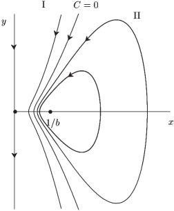
Figure 1: Phase portrait of (18)

4 Discussion

The periodic solutions of (18) induce periodicity to the full four-dimensional system (16) or (15). In fact, if $x\left(t\right)$ and $y\left(t\right)$ are periodic solutions, then (17) implies that the functions

$$u\left(t\right)=r\left(t\right)\cos\left(\tfrac{1}{\sqrt{6\beta}}t\right),\ \ \ w=r\left(t\right)\sin\left(\tfrac{1}{\sqrt{6\beta}}t\right)$$

oscillate in the $u-w$ plane with a periodic amplitude $r(t).$ Obviously one cannot assign a physical meaning to the new variables $\left(u,w,x,y\right)$ since the transformations (11) and (14) have “mixed” the original variables of (8) in a nontrivial way. However, the periodic character of the solutions of (15) whatever the physical meaning of the variables be, has the following interpretation. Close to the equilibrium of the original system (8), there exist periodic solutions for all variables. This implies that an initially expanding closed universe can avoid recollapse through an infinite sequence of successive expansions and contractions. This interesting result was not revealed in the Einstein frame [9]. Since the basin of attraction of all periodic trajectories of (18) is an open subset of the phase space, there is enough room in the set of initial data of (8) which lead to an oscillating scale factor. It should be interesting to investigate the late time evolution of closed FRW models in the Jordan frame by including matter satisfying some plausible energy conditions. This issue will be presented elsewhere.

References

- [1] A.A. Ruzmaikin and T.V. Ruzmaikina, Sov. Phys. Lett. JETP 30, 372 (1970).
- [2] J.E. Lidsey, S. Nojiri and S.D. Odintsov, JHEP 0206, 026 (2002); C. Charmousis and J.F. Dufaux, Class. Quant. Grav. 19, 4671 (2002); S. Mukohyama, Phys. Rev. D65, 084036 (2002); B. Abdesselam and N. Mohammedi, Phys. Rev. D65, 084018 (2002).
- [3] S. Carroll, V. Duvvuri, M. Trodden and M. Turner Phys. Rev. D70, 043528 (2004); T. Chiba Phys. Lett. B575, 1 (2003).
- [4] S. Carroll, Preprint astro-ph/0310342 (2003).
- [5] J.D. Barrow and S. Cotsakis, Phys. Lett. B214, 515 (1988); K. Maeda, Phys. Rev. D37, 858 (1988); S. Gottlöber, V. Müller, H. Schmidt and A. Starobinsky, Int. J. Mod. Phys. D2, 257 (1992).
- [6] G. Magnano and L.M. Sokolowski, Phys. Rev. D50, 5039 (1994).
- [7] V. Faraoni, E. Gunzig and P. Nardone, Fund. Cosmic Phys. 20, 121 (1999); S. Cotsakis, Preprint gr-qc/0408095 (2004).
- [8] J. Miritzis, J. Math. Phys. 44, 3900 (2003).
- [9] J. Miritzis, J. Math. Phys. 46, 082502 (2005).