A Measurement of Newton’s Gravitational Constant

Abstract

A precision measurement of the gravitational constant $G$ has been made using a beam balance. Special attention has been given to determining the calibration, the effect of a possible nonlinearity of the balance and the zero-point variation of the balance. The equipment, the measurements and the analysis are described in detail. The value obtained for $G$ is 6.674252(109)(54) $\times 10^{-11}$ $\mbox{m}^{3}\;\mbox{kg}^{-1}\;\mbox{s}^{-2}$. The relative statistical and systematic uncertainties of this result are 16.3$\times 10^{-6}$ and 8.1 $\times 10^{-6}$, respectively.

I Introduction

The gravitational constant $G$ has proved to be a very difficult quantity for experimenters to measure accurately. In 1998, the Committee on Data Science and Technology (CODATA) recommended a value of $6.673(10)\times 10^{-11}\;\mbox{m}^{3}\;\mbox{kg}^{-1}\;\mbox{s}^{-2}$. Surprisingly, the uncertainty, 1,500 parts per million (ppm), had been increased by a factor of 12 over the previously adjusted value of 1986. This was due to the fact that no explanation had been found for the large differences obtained in the presumably more accurate measurements carried out since 1986. Obviously, the differences were due to very large systematic errors. The most recent revision Mo05 of the CODATA Task Group gives for the 2002 recommended value $G=6.6742(10)\times 10^{-11}\;\mbox{m}^{3}\;\mbox{kg}^{-1}\;\mbox{s}^{-2}$. The uncertainty (150 ppm) has been reduced by a factor of 10 from the 1998 value, but the agreement among the measured values considered in this compilation is still somewhat worse than quoted uncertainties.

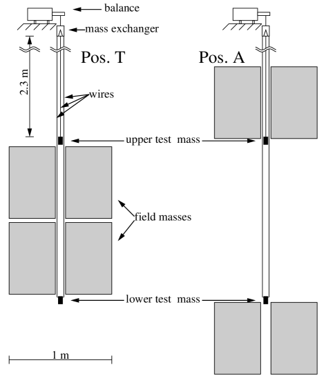
Figure 1: Principle of the measurement. The FM’s are shown in the position together (Pos. T) and the position apart (Pos. A).

Initial interest in the gravitational constant at our institute had been motivated by reports Fi86 suggesting the existence of a “fifth” force which was thought to be important at large distances. This prompted measurements at a Swiss storage lake in which the water level varied by 44 m. The experiment involved weighing two test masses (TM’s) suspended next to the lake at different heights. No evidence Co94 ; Hu95 was found for the proposed “fifth” force, but, considering the large distances involved, a reasonably accurate value (750 ppm) was obtained for $G$. It was realized that the same type of measurement could be made in the laboratory with much better accuracy with the lake being replaced by the well defined geometry of a vessel containing a dense liquid such as mercury. Equipment for this purpose was designed and constructed in which two 1.1 kg TM’s were alternately weighed in the presence of two moveable field masses (FM’s) each with a mass of 7.5 t. A first series of measurements Sa98 ; Sb98 ; No98 ; No99 ; Sa99 with this equipment resulted in a value for $G$ with an uncertainty of 220 ppm due primarily to a possible nonlinearity of the balance response function. A second series of measurements was undertaken to eliminate this problem. A brief report of this latter series of measurements has been given in ref. Sa02 and a more detailed description in a thesis Sb02 . Since terminating the measurements, the following four years have been spent in improving the analysis and checking for possible systematic errors.

Following a brief overview of the experiment, the measurement and the analysis of the data are presented in Secs. III entitled Measurement of the Gravitational Signal and Sec. IV entitled Determination of the Mass-Integration Constant. In Sec. V, the present result is discussed and compared with other recent measurements of the gravitational constant.

II General Considerations

The design goal of this experiment was that the uncertainty in the measured value of $G$ should be less than about 20 ppm. This is comparable to the quoted accuracy of recent $G$ measurements made with a torsion balance. It is, however, several orders of magnitude better than previous measurements of the gravitational constant (made after 1898) employing a beam balance Hu95 ; Mo88 ; Sp87 .

The experimental setup is illustrated in Fig. 1. Two nearly identical 1.1 kg TM’s hanging on long wires are alternately weighed on a beam balance in the presence of the two movable FM’s weighing 7.5 t each. The position of the FM’s relative to the TM’s influence the measured weights. The geometry is such that when the FM are in the position labelled ”together”, the weight of the upper TM is increased and that of the lower TM is decreased. The opposite change in the TM weights occurs when the FM are in the position labelled ”apart”. One measures the difference of TM weights first with one position of the FM’s and then with the other. The difference between the TM weight differences for the two FM positions is the gravitational signal.

The use of two TM’s and two FM’s has several advantages over a single TM and a single movable FM. Comparing two nearly equivalent TM’s tends to cancel slow variations such as zero-point drift of the balance and the effect of tidal variations. Using the difference of the two TM weights doubles the signal. In addition, it causes the influence of the FM motion on the counter weight of the balance to be completely cancelled. Use of two FM’s with equal and opposite motion reduces the power required to that of overcoming friction. This also simplified somewhat the mechanical construction.

The geometry has been designed such that the TM being weighed is positioned at (or near) an extremum of the vertical force field in both the vertical and horizontal directions for both positions of the FM’s. The extremum is a maximum for the vertical position and a minimum for the horizontal position. This double extremum greatly reduces the positional accuracy required in the present experiment.

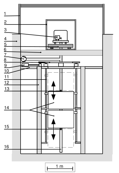
Figure 2: A side view of the experiment. Legend: 1=measuring room enclosure, 2=thermally insulated chamber, 3=balance, 4=concrete walls of the pit, 5=granite plate, 6=steel girder, 7=vacuum pumps, 8=gear drive, 9=motor, 10=working platform, 11=spindle, 12=steel girder of the main support, 13=upper TM, 14=FM’s, 15=lower TM, 16=vacuum tube.

The measurement took place at the Paul Scherrer Institut (PSI) in Villigen. The apparatus was installed in a pit with thick concrete walls which provided good thermal stability and isolation from vibrations. The arrangement of the equipment is shown in Fig. 2. The system involving the FM’s was supported by a rigid steel structure mounted on the floor of the pit. Steel girders fastened to the walls of the pit supported the balance, the massive (200 kg) granite plate employed to reduce high frequency vibrations and the vacuum system enclosing the balance and the TM’s. A vacuum of better than $10^{-4}$ Pa was produced by a turbomolecular pump located at a distance of 2 m from the balance.

The pit was divided into an upper and a lower room separated by a working platform 3.5 m above the floor of the pit. All heat producing electrical equipment was located in the upper measuring room. Both rooms had their own separate temperature stabilizing systems. The long term temperature stability in both rooms was better than $0.1^{\circ}$ C. No one was allowed in either room during the measurements in order to avoid perturbing effects.

The equipment was fully automated. Measurements lasting up to 7 weeks were essentially unattended. The experiment was controlled from our Zurich office via the internet with data transfer occurring once a day.

III Measurement of the Gravitational Signal

We begin this section with a description of the devices employed in determining the gravitational signal. Following the descriptions of these devices, the detailed schedule of the various weighings and their analysis are given. Balance weighings will be expressed in mass units rather than force units. The value of local gravity was determined for us by E. E. Klingelé of the geology department of the Swiss Federal Institute. The measurement was made near the balance on Sept. 11, 1996 using a commercial gravimeter (model G #317 made by the company LaCoste-Romberg). The value found was $9.8072335(6)\;\mbox{m}\mbox{s}^{-2}$. This value was used to convert the balance readings into force units.

III.1 The Balance

The beam balance was a modified commercial mass comparator of the type AT1006 produced by the Mettler-Toledo company. The mass being measured is compensated by a counter weight and a small magnetic force between a permanent magnet and the current flowing in a coil mounted on the balance arm. An opto-electrical feedback system controlling the coil current maintains the balance arm in essentially a fixed position independent of the mass being weighed. The digitized coil current is used as the output reading of the balance.

The balance arm is supported by two flexure strips which act as the pivot. The pan of the balance is supported by a parallelogram guide attached to the balance frame. This guide allows only vertical motion of the pan to be coupled to the arm of the balance. Horizontal forces produced by the load are transmitted to the frame and have almost no influence on the arm.

As supplied by the manufacturer, the balance had a measuring range of 24 g above the 1 kg offset determined by the counter weight. The original readout resolution was 1 $\mu$g and the specified reproducibility was 2 $\mu$g. The balance was designed especially for weighing a 1 kg standard mass such as is maintained in many national metrology institutes.

In the present experiment, the balance was modified by removing some nonessential parts of the balance pan which resulted in its weighing range being centered on 1.1 kg instead of the 1 kg of a standard mass. Therefore, 1.1 kg TM’s were employed. In order to obtain higher sensitivity required for measuring the approximately 0.8 mg difference between TM weighings, the number of turns on the coil was reduced by a factor of 6, thus reducing the range to 4 g for the same maximum coil current. The balance was operated at an output value near 0.6 g which gave a good signal-to-noise ratio with low internal heating. For the present measurements, a mass range of only 0.2 g was required. The full readout resolution of the analog to digital converter (ADC) measuring the coil current was employed which resulted in a readout-mass resolution of 12.5 ng.

An 8th order low-pass, digital filter with various time constants was available on the balance. Due to the many weighings required by the procedure employed to cancel nonlinearity (see Sec. III.4), it was advantageous to make the time taken for each weighing as short as possible. Therefore, the shortest filter time constant (approximately 7.8 s) was employed and output readings were taken at the maximum repetition rate allowed by the balance (about 0.38 s between readings).

Pendulum oscillations were excited by the TM exchanges. Small oscillation amplitudes (less than 0.2 mm) of the TM’s corresponding to one and two times the frequency for pendulum oscillations (approximately 0.26 Hz for the lower TM and 0.33 Hz for the upper TM’s) were observed. They were essentially undamped with decay times of several days. The unwanted output amplitudes of these pendulum oscillation were not strongly attenuated by the filter (half-power frequency of 0.13 Hz) and therefore had to be taken into account in determining the equilibrium value of a weighing.

The equilibrium value of a weighing was determined in an on-line, 5-parameter, linear least-squares fit made to 103 consecutive readings of the balance starting 40 s after a load change. The parameters of the fit were 2 sine amplitudes, 2 cosine amplitudes and the average weight. The pendulum frequencies were known from other measurements and were not parameters of the on-line fit. The 40 s delay before beginning data taking was required in order to allow the balance to reach its equilibrium value (except for oscillations) after a load change. This procedure (including the 40 s wait) is what we call a ”weighing”. A weighing thus required about 80 s.

Data of a typical weighing and the fit function used to describe their time distribution are shown in the upper part of Fig. 3. The residuals $\delta$ divided by a normalization constant $\sigma$ are shown in the lower part of this figure. The normalization constant has been chosen such that the rms value of the residuals is 1. Since the balance readings are correlated due to the action of the digital filter, the value of $\sigma$ does not represent the uncertainty of the readings. It is seen that the residuals show only rather wide peaks. These peaks are probably due to very short random bursts of electronic noise which have been widened by the digital filter. With the sensitivity of our modified balance, they represent a sizable contribution to the statistical variations of the weighings. They are of no importance for the normal use of the AT1006 balance.

Figure 3: Shown in the upper plot are the balance readings for a typical weighing illustrating the oscillatory signal due to pendulum oscillations. The output is the uncalibrated balance reading corresponding to approximately 1.1 kg with a magnetic compensation of 0.6 g. The amplitude of the oscillatory signal corresponds to about 1.5 $\mu$g. The lower plot shows the normalized residuals. The normalization has been chosen such that their rms value is 1.

A direct calibration of the balance in the range of the 780 $\mu$g gravitation signal can not be made with the accuracy required in the present experiment ($<20$ ppm) since calibration masses of this size are not available with an absolute accuracy of better than about 300 ppm. Instead, we have employed a method in which an accurate, coarse grain calibration was made using two 0.1 g calibration masses (CM’s). The CM’s were each known with an absolute accuracy of 4 ppm. A number of auxiliary masses (AM’s) having approximate weights of either 783 $\mu g$ or $16\times 783=12,528$ $\mu$g were weighed along with each TM in steps of 783 $\mu$g covering the 0.2 g range of the CM. Although the AM’s were known with an absolute accuracy of only 800 ng (relative uncertainty 1,000 ppm), the method allowed balance nonlinearity effects to be almost entirely cancelled. Thus, the effective calibration accuracy for the average of the TM difference measurements was essentially that of the CM’s. A detailed description of this method is given in Sec. III.10.

In our measurements, the balance was operated in vacuum. The balance proved to be extremely temperature sensitive which was exacerbated by the lack of convection cooling in vacuum. The measured zero-point drift was 5.5 mg/${}^{\circ}\mbox{C}$. The sensitivity of the balance changed by 220 ppm$/^{\circ}\mbox{C}$. To reduce these effects, the air temperature of the room was stabilized to about 0.1 ${}^{\circ}\mbox{C}$. A second stabilized region near the balance was maintained at a constant temperature to 0.01 ${}^{\circ}\mbox{C}$. Inside the vacuum, the balance was surrounded by a massive (45 kg) copper box which resulted in a temperature stability of about 1 mK. Although zero-point drift under constant load for a 1 mK temperature change was only 5.5 $\mu$g , the effects of self heating of the balance due to load changes during the measurement of the gravitational signal were much larger. Details of this effect and how they were corrected are described in Sec.III.7.

III.2 The Test Masses

One series of measurements was made using copper TM’s and two with tantalum TM’s. Various problems with the mass handler occurred during the measurements with the tantalum TM’s which resulted in large systematic errors. Although the tantalum results were consistent with the measurements with the copper TM’s, the large systematic errors resulted in large total errors. The tantalum measurements were included in our first publication, but we now believe that better accuracy is obtained overall with the copper measurements alone. We therefore describe only the measurements made with the copper TM’s in the present work.

A drawing of a copper TM is shown in Fig. 4. The 45 mm diameter, 77 mm high copper cylinders were plated with a 10 $\mu$m gold layer to avoid oxidation. The gold plating was made without the use of nickel in order to avoid magnetic effects. Near the top of each TM on opposite sides of the cylinder were two short horizontal posts. The posts were made of Cu-Be (Berylco 25). The tungsten wires used to attach the TM’s to the balance were looped around these posts in grooves provided for this purpose. The wires had a diameter of 0.1 mm and lengths of 2.3 m for the upper TM and 3.7 m for the lower. The loop was made by crimping the tungsten wire together in a thin copper tube. A thin, accurately machined, copper washer was placed in a cylindrical indentation on the top surface of the lower TM in order to trim its weight (including suspension) to within about 400 $\mu$g of that of the upper TM and suspension.

Figure 4: Drawing of TM inside the vacuum tube. Dimensions are given in mm.

Measurement of the TM’s dimensions was made with an accuracy of 5 $\mu$m using the coordinate measuring machine (CMM) at PSI. The weight of the gold plating was determined from the specified thickness of the layer. The weight of the tungsten wires was determined from the dimensions and the density of tungsten. The thin tubing used to crimp the tungsten wires was weighed directly. The weight of the complete TM’s was determined at the Mettler-Toledo laboratory with an accuracy of 25 $\mu$g (0.022 ppm) before and after the gravitational measurement. It was found that the mass of both TM’s had increased by a negligible amount (0.5 ppm) during the measurement.

An estimate of possible density gradients in the TM’s was determined by measuring the density of copper samples bordering the material used for making the TM’s. It was found that the variation of the relative density gradients over the dimensions of either TM was less than $2\times 10^{-4}$ in both the longitudinal and the radial directions.

III.3 TM Exchanger

In weighing the TM’s, it was necessary to remove the suspension supporting one TM from the balance and replace it by the other supporting the other TM. The exchange was accomplished by a step-motor driven hydraulic systems to raise the suspension of one TM while lowering the other. A piezo-electric transducer mounted above the pan of the balance was used to keep the load on the balance during the exchange as constant as possible. This was done in order to avoid excessive heating due to the coil current and to reduce anelastic effects in the flexure strips supporting the balance arm. The output excursions were typically less than 0.1 g. The exchange of the TM’s required about 4 min.

The TM suspension rested on a thin metal arm designed to bend through 0.6 mm when loaded with 1.1 kg. Therefore, the transfer of TM’s was accomplished with a vertical movement of typically 2 mm (0.6 mm bending of the spring plus an additional 1.4 mm to avoid electrostatic forces). The metal arm was attached to a parallelogram guide (similar to that of the balance) to assure only vertical motion.

Although the parallelogram reduced the error resulting from the positioning of the load, it was nevertheless important to have the TM load always suspended from the same point on the balance pan. This was accomplished by means of a kinematic coupling Sl88 ; Fu81 . The coupling consisted of three pointed titanium pins attached to each TM suspension which would come to rest in three titanium V grooves mounted on the balance pan. The reproducibility of this positioning was 10 $\mu$m. The pieces of the coupling were coated with tungsten carbide to avoid electrical charging and reduce friction.

III.4 Auxiliary Masses

In order to correct for any nonlinearity of the balance in the range of the signal, use was made of many auxiliary masses (AM’s) spanning the 200 mg range of the CM’s in steps of approximately 783 $\mu$g. Although the AM’s could not be measured with sufficient accuracy to calibrate the balance absolutely, they were accurate enough to correct the measured gravitational signal for a possible nonlinearity of the balance. Each TM was weighed along with various combinations of AM’s. One essentially averaged the nonlinearity over the 200 mg range of the CM’s in 256 load steps of 200 mg/256=783 $\mu$g. A weighing of both 100 mg CM’s was then used to determine the absolute calibration of the balance which is valid for the TM weighings averaged over this range. The effect of any nonlinearity essentially cancels due to the averaging process. The accuracy of the nonlinearity correction is described in Sec. III.10.

The 256 load steps were accomplished using 15 AM’s with a mass of approximately 783 $\mu$g called AM1’s and 15 AM’s with 16 times this mass (12,528 $\mu$g) called AM16’s. They were made from short pieces of stainless steel wire with diameters of 0.1 mm and 0.3 mm. The wires were bent through about $70^{\circ}$ on both ends leaving a straight middle section of about 6 mm. The mass of the AM’s were electrochemically etched to obtain as closely as possible the desired masses. The RMS deviation was 1.5 $\mu$g for the AM1’s and 2.3 $\mu$g  for the AM16’s.

By weighing a TM together with various AM combinations, one obtains the value of the TM weight simultaneously with the linearity information. The only additional time required for this procedure over that of weighing only the TM’s is the time necessary to change an AM combination (10 to 30 s).

III.5 Mass Handler

The mass handler is the device which placed the AM’s and the CM’s on the balance or removed them from the balance. The mass handler was designed by the firm Metrotec AG. The operation of this device is illustrated in the somewhat simplified drawing of Fig. 5 showing how the AM1’s and the CM1 are placed on the metal strip attached to the balance pan. Only 6 of the 14 steps are shown in this illustration for clarity. The portion of the handler used for the AM’16 and the CM2 (not shown) is similar except that the AM’16 are placed on a metal strip located below the one used for the AM1’s. All of the AM1’s pictured in Fig. 5 are lying on the steps of a pair of parallel double staircases. The staircases are separated by 6 mm which is the width of the AM’s between the bent regions on both ends. The spacing between the staircases is such that they could pass on either side of the horizontal metal strip fastened to the balance pan as the staircases were moved up or down. The motion of each staircase pair was constrained to the vertical direction by a parallelogram (similar to those of the balance) fastened to the frame of the mass handler. The staircases for AM1’s and AM16’s were moved by two separate step motors located outside the vacuum system. The step motors were surrounded by mu metal shielding to reduce the magnetic field in the neighborhood of the balance. Moving the staircases down deposited one AM after another onto the metal strip. Moving the staircases up removed the AM’s lying on the strip. The steps of the staircase had hand filed, saddle shaped indentations to facilitate the positioning of the AM’s. The heights of the steps were 2 mm and the steps on the left side of the double staircase were displaced in height by 1 mm from those on the right. Thus, the AM1’s were alternately placed on the balance to the left and to the right of the center of the main pan in order to minimize the torque which they produced on the balance.

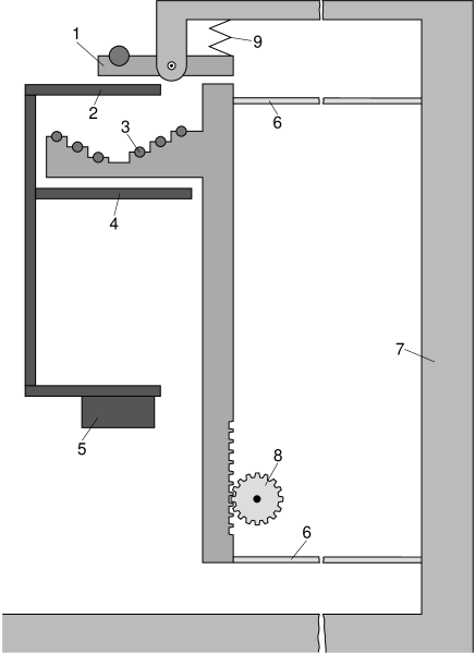
Figure 5: Simplified drawing of the mass handler illustrating the principle of operation. Legend: 1=pivoted lever pair holding a CM, 2=narrow strip to receive the CM, 3=double stair case pair holding AM’s, 4=narrow strip to receive AM’s, 5=balance pan, 6 flat spring, 7=frame, 8=stepmotor driven cogwheel, and 9=coil spring. The pivoted-lever pair and the double-staircase pair are spaced such that they can pass on either side of the narrow strips 2 and 4 fastened to the balance pan. The two flat springs 6 form two sides of a parallelogram which assures vertical motion of the double stair case pair.

Raising the staircase structure above the position shown in the figure caused a rod to push against a pivoted lever holding CM1. With this operation, CM1 was placed on the upper strip attached to the balance. Reversing the operation allowed the spring to move the lever in the opposite direction and remove CM1 from the balance.

Due to the very small mass of the AM1’s, difficulty was occasionally experienced with the AM1’s sticking to one side of the staircase or the other. The staircases were made of aluminum and were coated with a conductive layer of tungsten carbide to reduce the sticking probability. Sticking nevertheless did occur. The sticking would cause an AM1 to rest partly on the staircase and partly on the pan, thus giving a false balance reading. In extreme cases, the AM1 would fall from the holder and therefore be lost for the rest of the measurement. No problem was experienced with the heavier AM16’s and the CM’s.

III.6 Weighing Schedule

The experiment was planned so that the zero-point (ZP) drift and the linearity of the balance could be determined while weighing a TM. In principle one needs just 4 weighings (upper and lower TM with FM’s together and apart) to determine the signal for each AM placed on the balance. Repeating these 4 weighings allows one to determine how much the zero point has changed and thereby correct for the drift. Since there are 256 AM values required to correct the nonlinearity of the balance, a minimum of 2048 weighings is needed for a complete determination of the signal corrected for ZP drift and linearity. One also wishes to make a number of calibration measurements during the series of measurements.

The order in which the measurements are performed influences greatly the ZP drift correction of measurements. Changing AM’s requires only 6 to 30 s, while exchanging TM on the balance takes about 230 s and moving the FM from one position to the other requires about 600 s. These times are to be compared with the 80 s required for a weighing and about 1 hr for a complete calibration measurement (see Sec. III.9). One therefore wishes to measure a number of AM values before exchanging TM, and repeat these measurements for the other TM before changing the FM positions or making a calibration.

The schedule of weighing adopted is based on several basic series for the weighing of the different TM’s with different FM positions. The series are defined as follows:

1. An S4 series is defined as the weighing of four successive AM values with a particular TM and with all weighing made for the same FM positions.

2. An S12 series involves three S4 series all with the same four AM values and the same FM positions. The S4 series are measured first for one TM, then the other TM and finally with the original TM.

3. An S96 is eight S12 series, all made with the same FM positions and with the AM values incremented by four units between each S12 series. A TM exchange is also made between each S12 series. An S96 series represents the weighings with 32 successive AM values for both TM all with the same FM positions.

4. An S288 series is three S96 series, first with one FM position, then the other and finally with the original FM position. A calibration measurement is made at the beginning of each S288 series. Thus, the S288 series represents the weighings with 32 successive AM values for both TM’s and both FM positions and includes its own calibration.

5. An S2304 series is made up of eight S288 series with the AM values incremented by 32 between each S288 series. An S2304 series completes the full 256 AM values with weighings of both TM’s and both FM positions.

A total of eight valid S2304 series was made over a period of 43 days. Alternate S2304 series were intended to be made with increasing and decreasing AM values. Unfortunately, the restart after a malfunction of the temperature stabilization in the measuring room was made with the wrong incrementing sign. This resulted in five S2304 series being made with increasing AM values and three with decreasing.

III.7 Analysis of the Weighings

In ref. Sa02 ; Sb02 , the so called ABA method was used to analyze the data obtained from the balance and thereby obtain the difference between the mass of the A and B TM. This method assumes a linear time dependence of the weight that would be obtained for the A TM at the time when the B TM was measured based on the weights measured for A at an earlier and a later time. However, a careful examination of the data showed that the curvature of the ZP drift was quite large and was influenced by the previous load history of the balance. This indicated that the linear approximation was not a particularly good approximation. We have therefore reanalyzed the data using a fitting procedure to determine a continuous ZP function of time for each S96 series. The data and fit function for a typical S96 series starting with a calibration measurement is shown in Fig. 6. The procedure used to determine the ZP data and fit are described in the following. The criterion for a valid weighing is described in Sec. III.8.

The data of Fig. 6 show a slow rise during the first hour after the calibration measurement followed by a continuous decrease with a time constant of several hours. These slow variations are attributed to thermal variations resulting principally from the different loading of the balance during the calibration measurement. Superposed on the slow variations are rapid variations which are synchronous with the exchange of the TM’s. The rapid variations peak immediately after the TM exchange and decrease thereafter with a typical slope of 0.3  $\mu$g /hr. The cause of the rapid variations is unknown.

The data employed in the ZP determination were the weighings of the upper and lower TM’s for the S96 series. The known AM load for each weighing was first subtracted to obtain a net weight for either TM plus the unknown zero-point function at the time of each weighing. A series of Legendre polynomials was used to describe the slow variations of the zero-point function. A separate $P_{0}$ coefficient was employed for each TM. The rapid variations were described by a sawtooth function starting at the time of each TM exchange. The fit parameters were the coefficient of the Legendre polynomials and the amplitude of the sawtooth function. The sawtooth amplitude was assumed to be the same for all rapid peaks of an S96 series. The sawtooth function was used principally to reduce the $\chi^{2}$ of the fit and had almost no effect on the results obtained when using the ZP function. All parameters are linear parameters so that no iteration is required. The actual ZP function is the sawtooth function and the polynomial series exclusive of the time independent terms (i.e. the sum of the coefficients times $P_{n}(0)$ for even $n$).

Figure 6: The zero-point variation as a function of time for a typical S96 series including calibration is shown in the upper part of this figure. The solid curve is the fit function starting after the last dummy weighing. The fit function for this S96 series has 76 degrees of freedom. The normalized residuals $\delta/\sigma$ are shown in the lower plot. The normalization of the residuals has been chosen such that their rms value is 1.

Such calculations were made for various numbers of Legendre coefficients in the ZP function. It was found that the gravitational signal was essentially constant for a maximum order of Legendre polynomials between 8 and 36. In this range of polynomials, the minimum calculated signal was 784.8976(91) $\mu$g for a maximum order equal to 22 and a maximum signal of 784.9025(93) $\mu$g for a maximum order equal to 36 (i.e. a very small difference). In all following results, we shall use the signal 784.8994(91) $\mu$g obtained with a maximum polynomial order of 15.

It has been implicitly assumed in the above ZP determination that the AM load values were known with much better accuracy than the reproducibility of the balance producing the data used in the ZP fit. Although the AM values were sufficiently accurate for determining the general shape of the ZP function, their relative uncertainties were comparable to the uncertainties of the balance data used in the fit. The $P_{0}$ mass parameters of the TM’s obtained from the fit were therefore not used for the TM differences at the two FM positions which are needed in order to determine the gravitational signal. Instead, the value of the ZP function was subtracted from each weighing, and an ABA mass difference was determined for each triplet of weighings having the same AM load. Since the mass of the AM’s do not occur in this TM difference, they do not influence the calculation. The ABA calculation is valid for this purpose since the ZP corrected weighings have essentially no curvature. Such TM differences determined for the apart-together positions of the FM’s are then used to calculate the gravitational signal.

The TM differences for the apart-together positions of the FM’s as a function of time are shown for a ZP corrected S288 series in Fig. 7. Individual data points are resolved in the magnified insert of this figure. Each data point is the B member of a TM difference obtained from an ABA triplet in which all weighings have the same load value.

Figure 7: The measured weight difference in $\mu g$ between TM’s obtained from an S288 series. The magnified insert shows the individual TM differences which are not resolved in the main part of the figure.

All of the TM differences (ZP corrected) for the entire experiment are shown in Fig. 8. The data labelled apart have been shifted by 782 $\mu$g in order to allow both data sets to be presented in the same figure. A slow variation of 2.5 $\mu$g in both TM differences occurred during the 43 day measurement. Also seen in this figure is a 0.7 $\mu$g jump which occurred in the data for both the apart and together positions of the FM’s on day 222. The slow variation is probably due to sorption-effect differences of the upper and lower TM’s. The jump was caused by the loss or gain of a small particle such as a dust particle by one of the TM’s. In order to determine the gravitational signal, an ABA difference was calculated for apart-together values having the same AM load. The slow variation seen in Fig. 8 is sufficiently linear so that essentially no error results from the use of the ABA method. The jump in the apart-together differences caused no variation of the gravitational signal.

Figure 8: The measured weight difference in $\mu g$ between TM’s for the FM’s positions apart and together. The measured values for the FM apart have been displaced 782 $\mu g$ in order to show both types of data in the same figure.

In Fig. 9 is shown a plot of the binned difference between the FM apart-together positions for all valid data (see Sec. III.8. The differences were determined using the ABA method applied to weighings made with the same AM loads. Also shown in the figure is a Gaussian function fit to the data. The data are seen to agree well with the Gaussian shape which is a good test for the quality of experimental data. The root-mean-square (RMS) width of the data is 1.03 time the width of the Gaussian function. The true resolution for these weighings may be somewhat different than shown in Fig. 9 due to the fact that the data have not been corrected for nonlinearity of the balance (see Sec. III.10) and for correlations due to the common ZP function . Nevertheless, these effects would not be expected to influence the general Gaussian form of the distribution.

Figure 9: Binned data for the FM apart-together weight differences (points) and a fitted Gaussian function (curve) shown as a deviation from the mean difference. Poisson statistics were used to determine the uncertainties.

A plot of the signal obtained for the S2304 series with increasing and decreasing load is shown in Fig. 10. The average signal for increasing load is 784.9121(125) $\mu$g and the average for decreasing load is 784.8850(133) $\mu$g. The common average for both is 784.8994(91) $\mu$g. The averages for increasing load and for decreasing load lie within the uncertainty of the combined average. This shows that the direction of load incrementing did not appreciably influence the result.

Figure 10: The average signal for each of the eight S2304 series. Series with increasing load are shown as circles. Series with decreasing load are shown as squares. The dashed line is the average of all eight series.

Although the weighings making up an S96 series are correlated due to the common ZP function determined for each S96 series, the results of each S96 series, in particular the TM parameter, are independent. The 32 signal values obtained from the three S96 series making each S288 series are also independent. However, since the nonlinearity correction (see Sec. III.10) being employed is applicable only to an entire S2304 series (not to individual S288 series), it is only the eight S2304 series which should be compared with one another. This restricts the way in which the average signal is to be calculated for the entire measurement, namely the way in which the data are to be weighted.

We have investigated two weighting procedures. In the first, each S2304 series average was weighted by the number of valid triplets in that series. This assumes that the weighings measured in all S2304 series have the same a priori accuracy. In the second method, it was assumed that the accuracy for each weighing in a series was the same but might be different for different series. We believe the second method is the better method since it takes into account changes that occur during the long, 43 day measurement (e.g. the not completely compensated effects of vibration, tidal forces and temperature). The averages obtained with the two methods differ by approximately 6 ng with the second method giving the smaller average signal. This is a rather large effect. It is only slightly smaller than the statistical uncertainty of 9 to 10 ng obtained for either method. In the rest of this work, we shall discus only the results obtained with the second method.

III.8 Criterion for Valid Data

Two tests were used to determine whether a measured weighing was valid. An on-line test checked whether the $\chi^{2}$ value of the fit to the pendulum oscillations was reasonable. A large value caused a repeat of the weighing. After two repeats with large $\chi^{2}$, the measurement for this AM value was aborted. An aborted weighing usually indicated that the AM was resting on the mass handler and on the balance pan in an unstable way.

A more frequent occurrence was that of an AM which rested on both the mass handler and the balance was almost stable thereby giving a reasonable $\chi^{2}$. In order to reject such weighings, an off-line calculation was made to check whether the measured weight was within 10 $\mu$g of the expected weight. The statistical noise of a valid weighing was typically about 0.15 $\mu$g (see Fig. 9 showing ABA difference involving 3 weighings). Excursions of more than 10 $\mu$g were thus a clear indication of a malfunction.

This off-line test is somewhat more restrictive than the off-line test employed in our original analysis. In the original analysis, a check was made only to see that the weight difference between the TM’s for equal AM loadings was reasonable. The more restrictive test used in the present analysis resulted in the rejection of the S2304 series at the time when the room temperature stabilizer was just beginning to fail. It was also the reason for not including the tantalum TM-measurements in the present analysis. In the eight S2304 series accepted for the determination of the gravitational constant, approximately 8% of the expected zero-point values could not be determined due to at least one of the three weighings at each load value being rejected by the test for valid weighings.

III.9 Calibration Measurements

A coarse calibration of the balance was made periodically during the gravitational measurement (before each S288 series) using two calibration masses each with a weight of approximately 100 mg. A correction to the coarse calibration constant due to the nonlinearity of the balance will be discussed in Sec. III.10. The two CM’s used for the coarse calibration were short sections of stainless steel wire. The diameter of CM1 was 0.50(1) mm and that of CM2 was 0.96(1) mm. The surface area of CM1 was approximately 1 cm² and that of CM2 was 0.5 cm². The CM’s were electrochemically etched to the desired mass and then cleaned in an ethanol ultrasonic bath. The mass of each CM was determined at METAS (Metrology and Accreditation Switzerland) in air with an absolute accuracy of 0.4 $\mu$g  or a relative uncertainty of 4 ppm. The absolute determinations of the CM masses were made before and after the gravitational measurement with copper TM’s and after the second measurement with tantalum TM’s. Only the first measurement was used to evaluate the coarse calibration constant employed in the measurement with copper TM’s. As will be discussed below, the second and third measurement were used for the measurement with copper TM’s only to check the stability of the CM’s.

A calibration measurement involved either TM and one of following seven additional loads: (1) CM1 alone, (2) CM2 alone, (3) again CM1 alone, (4) empty balance, (5) CM1+CM2, (6) empty balance and (7) CM1+CM2 and nine so called dummy weighings. These measurements were made with no AM’s on the balance. After the seventh weighing, a series of nine dummy weighings alternating between upper and lower TM’s were made with the AM load set to the value for the next TM weighing. The dummy weighings were made in order to allow the balance to recover from the large load variations experienced during the calibration measurement and thereby come to an approximate equilibrium value before the next TM weighing. Calibrations were made alternately with the upper and lower TM’s as load. Calibration measurements were made about twice a day. Including the dummy weighings, each calibration required about 50 min.

A three-parameter least squares fit was made to the calibration weighings labelled 4,5,6 and 7 above. The fit thereby determined best values for the balance ZP, the slope of the ZP and a parameter representing the effective ZP corrected reading of the balance for the load CM1+CM2. This third parameter is of particular interest since the coarse calibration constant is determined from the known mass of CM1+CM2 (measured by METAS) divided by this parameter. Therefore, the results of the least-squares fit to each set of calibration data gave a value for the coarse calibration constant which then was used to convert the balance output of the S288 series to approximate mass values. An ABA analysis of the first three weighings of each set of calibration data was also made in order to determine the difference in mass between CM1 and CM2.

The absolute masses obtained for CM1 and CM2 as determined by METAS are given in columns 2 and 3 of Table 1. Also shown in Table 1 (column 4) are the mass difference between CM1 and CM2 as obtained from the METAS measurement in air and the average of our CM measurement in vacuum. The mass differences between CM1 and CM2 measured in vacuum are particularly useful in checking for any mass variation of the CM’s.

Table 1: The mass of the CM’s as measured by METAS and the CM1-CM2 mass differences measured in air at METAS and in vacuum during the gravitational measurements at PSI. All values are given in $\mu g$.

Date	CM1	CM2	Difference
Feb 6, 01	100,270.30(40)	100,263.90(40)	6.40(60)
Jul. - Sep., 01	in vacuum		5.853(19)
Nov. 29, 01	100,270.20(35)	100,262.90(35)	7.30(50)
Jan. - Mar., 02	in vacuum		7.269(29)
Apr. - May, 02	in vacuum		7.496(25)
May 27, 02	100,270.01(35)	100,262.97(35)	7.04(50)

It is seen that CM2 mass decreased by 1.00(53) $\mu$g between the first and second METAS measurements while the mass of CM1 was essentially the same in all three measurements. From the mass difference values in air and vacuum it is clear that the change occurred after the measurements with copper TM’s ended in Sept. 2001 and before the weighing at METAS in Nov. 2001 which preceded the start of the tantalum measurements. We ascribe this change of CM2 to either the loss of a dust particle or perhaps a piece of the wire itself. The loss of a piece of the wire was possible since the wire used for the CM’s had been cut with a wire cutter and there could have been a small broken piece that was not bound tightly to the wire. For this reason only the values given for the first weighing of the CM’s were used to determine the coarse calibration constant used for the measurement with copper TM’s.

A plot of the relative change of the effective ZP corrected balance reading corresponding to the load CM1+CM2 is shown in Fig. 11. It is seen that it changed by only a few ppm over the 43 days of the measurement. A linear fit made to these data results in a slope equal to -0.044(6) ppm/day which is equivalent to a mass rate variation of -0.0088(12) $\mu$g cm^-2  d^-1. The uncertainty was obtained by normalizing $\chi^{2}$ of the fit to the degrees of freedom (DOF).

Figure 11: The change of the effective balance reading for the load CM1+CM2 as a function of time relative to its value on the first day. No valid measurements were made between day 229 and 235.

The slow variation of the effective balance reading for the load CM1+CM2 seen in Fig. 11 could be due either to a change of the balance sensitivity, to a decrease in the mass of CM1+CM2 due to the removal of a contaminant layer from the CM’s in vacuum or to a combination of both causes. A variation of the balance sensitivity would have essentially no effect on the analysis of the weighing for the gravitational measurement as the coarse calibration constant used for the analysis was determined from the balance parameter for each S288 series. However, a variation of the mass of CM1+CM2 would result in an error in the analysis since the mass would not be the value measured by METAS shown in Table 1.

In order to investigate this problem, we have examined the difference between the balance readings for CM1 and CM2. This difference is proportional to the surface areas of CM1 and CM2 which differ by approximately a factor of 2 (CM1 area=1 cm² and CM2 area=0.5 cm²). The balance reading difference is only slightly dependent upon the coarse calibration constant so that it represents essentially the mass difference itself. In Fig 12 is shown the measured mass difference as a function of time during the gravitational measurement. Also shown is a linear function fit to these data. The slope parameter of the fit results in a rate of increase per area equal to 0.0021(18) $\mu$g cm^-2  d^-1. The uncertainty has been determined by normalizing $\chi^{2}$ to the DOF. The sign of the slope is such that the CM with the larger area has the larger rate of increase. A mass difference variation (CM1-CM2) would require a slope of -0.0088(12) $\mu$g cm^-2  d^-1. The measured slope of the effective balance reading for the load CM1+CM2 clearly excludes such a large negative slope as assumed for a mass variation. We therefore conclude that the variation of this parameter is due primarily to the sensitivity variation of the balance.

We note that Schwartz Sch94b has also found a mass increase for stainless steel samples in a vacuum system involving a rotary pump, a turbomolecular pump and a liquid nitrogen cold trap. His samples were 1 kg masses with surface areas differing by a factor of 1.8. He measured the thickness of a contaminant layer using ellipsometry as well as the increase in weight of the sample during pumping periods of 1.2 d and 0.36 d. The rate of mass increase per area which he reports is approximately a factor of 5 larger than the value we find. No explanation for this difference can be made without a detailed knowledge of the partial pressures of the various contaminant gases in the two systems and the surface properties of the samples employed.

Figure 12: The mass difference of the CM’s as a function of time and the linear fit function.

There still remains the possibility that a rapid removal of an adsorbed layer such as water might have occurred between the absolute determination of the CM masses in air at METAS and the gravitational measurement in vacuum (i.e. during the pump down of the system). Schwartz Sch94a has measured the mass variation per unit area of 1 kg stainless steel objects in air with relative humidity between 3% and 77%. He Sch94b also has measured the additional mass variation per area due to pumping the system from atmospheric pressure at 3% relative humidity down to $5\times 10^{-3}$ Pa. His samples were first cleaned by wiping them with a linen cloth soaked in ethanol and diethylether and then ultrasonic cleaning in ethanol. After cleaning, they were dried in a vacuum oven at 50 ^∘C. For these cleaned samples, the weight change found for 3% to 50% humidity variation was 11.5 ng  cm^-2 with an additional change of 29 ng  cm^-2 in going from 3% relative humidity in air to vacuum (total change of 40.5 ng cm^-2). Similar measurements with ”uncleaned” samples gave a total change of 80 ng cm^-2. The variation due to the cleanliness of the samples was much larger than the difference found for the two types of stainless steel investigated and the effect of improving the surface smoothness (average peak-to-valley height equal to 0.1 $\mu$m  and 0.024 $\mu$m). Since the cleaning procedure used for our CM’s and their smoothness were different than the samples used by Schwartz, we have employed the average of Schwartz’s ”cleaned” and ”uncleaned” objects for estimating the mass change of our CM’s. Based on these data, the relative mass difference found for both CM’s together as measured in air having 50% humidity and in vacuum was 0.5 ppm. We assign a relative systematic uncertainty of this correction equal to the correction itself.

III.10 Nonlinearity Correction

By nonlinearity of the balance, one is referring to the variation of the balance response function with load, that is, the degree to which the balance output is not a linear function of the load. The nonlinearity of a mass comparator similar to the one employed in the present work has been investigated Re00 by the firm Mettler-Toledo. It was found that besides nonlinearity effects in 10 g load intervals, there was also a fine structure of the nonlinearity in the 0.1 mg load interval which would be important for the accuracy of the present measurement. It is the nonlinearity of our mass comparator in the particular load interval less than 0.2 g involved in the present experiment that we wish to determine.

One expects the nonlinearity of the balance used in this experiment to be small; however, it should be realized that a 200 mg test mass (two 100 mg CM’s) required for having an accurately known test mass for calibration purposes is over 250 times the size of the gravitational signal that one wishes to determine. In addition, the statistical accuracy of the measured gravitational signal is some 30 times better than the specified accuracy (2 $\mu$g) of the unmodified commercial balance. One therefore has no reason to expect the nonlinearity of the balance to be negligible with this precision. In Sec. III.1 we have presented the general idea that the measurements with 256 AM values tends to average out the effect of any nonlinearity. We wish now to give a more detailed analysis of this problem.

Figure 13: The $\chi^{2}$ probability as a function of the number of parameters.

The correction for nonlinearity makes use of an arbitrary response as a function of the load. Since the two TM’s are essentially equal ($<400$ $\mu$g  difference), the variation of the response function can be thought of as being a function of the additional load due to the AM’s. Although a power series or any polynomial series would suffice for this function, we have for convenience used a series of Legendre polynomials

$$f(u)=\sum_{\ell=0}^{Lmax}a_{\ell}P_{\ell}(2u/u_{max}-1).$$

The coefficients of $P_{\ell}$ are chosen subject to the two conditions that (1) $f(u)=0$ for no load and (2) $f(u)=C$ for $u=C$ where $C$ is the weight of the two CM’s together. These two conditions represent the sensitivity of the balance over the 0.2 g range of the calibration (i.e. the coarse calibration). The value of the maximum load $u_{max}$ in the present measurements was very nearly $C$. Substituting the above conditions into the response function, one obtains for the lowest two coefficients the expressions

$$a_{0}=C/2-\sum_{even\;\ell=2}^{Lmax}a_{\ell}$$

and

$$a_{1}=C/2-\sum_{odd\;\ell=3}^{Lmax}a_{\ell}.$$

One can then minimize

$$\chi^{2}=\sum_{n=1}^{N}\left[f(u_{n}+s)-f(u_{n})-y_{n}\right]^{2}\sigma_{n}^{-2}$$

and thereby determine best values for the parameters $s$ and $a_{\ell}$ for $\ell=1$ to $Lmax$. The $y_{n}$ are the measured balance signal for the load values $u_{n}$, $s$ is the load independent signal and $N$ is the number of different loads with valid measurements. The error $\sigma_{n}$ for the load value $u_{n}$ is the load-independent intrinsic noise of the balance $\sigma_{0}$ for a single weighing divided by the square root of the number of weighings for the load $u_{n}$. The value of $Lmax$ must be chosen large enough to describe the response function accurately. All of the parameters in the fit are linear parameters with the exception of $s$. Thus, there is no difficulty in extending the fit to a large number of parameters since only the nonlinear parameter must be determined by a search method.

In order to determine $Lmax$, we calculate the $\chi^{2}$ probability Ba89 (often referred to as confidence level) as a function of $Lmax$. This requires an approximate value for the intrinsic noise of the balance $\sigma_{0}$. The value of $\sigma_{0}$ sets the scale of the $\chi^{2}$ probability but does not change the general shape of the function. One can obtain a reasonable approximation for $\sigma_{0}$ by setting $\chi^{2}$ equal to the DOF obtained for a large number of parameter. We have arbitrarily set $\chi^{2}$ equal to the DOF for 61 parameters. The $\chi^{2}$ probability as a function of the maximum number of parameters is shown in Fig. 13. It is seen that the $\chi^{2}$ probability reaches a plateau near this maximum number of parameters.

Starting from a low value of $10^{-4}$ for one parameter, the $\chi^{2}$ probability rises rapidly to a value of 0.05 for three parameters. It remains approximately constant at this value up to 57 parameters where it rises sharply to reach a plateau of approximately 0.5 at 60 parameters and above. The fit parameter representing the signal corrected for nonlinearity of the balance was essentially constant over the entire range of parameters with a variation of less than $\pm 1.3$ ng. The signal for one parameter representing complete linearity was 784.8994 $\mu$g. The signal of the plateau region from 60 to 67 parameters was 784.9005 $\mu$g with a statistical uncertainty of 5.5 ng. In this region the signal varied by less than 0.2 ng. We therefore take the nonlinearity correction of the measured signal to be 1.1(5.5) ng (i.e. the difference between the signal using one parameter as would be obtained with no correction and the average value obtained for 60 to 67 parameters).

Figure 14: Signal and fit function employing 60 parameters as a function of load. The data are shown as a stepped line. The fit is the smooth curve. The lower plot shows the normalized residuals. Residuals were divided by the relative uncertainty of each point. The normalization has been chosen such that the rms value of the residuals is 1.

The nonlinear signal and fit as a function of load determined for 60 parameter is shown in Fig. 14. The function shows many narrow peaks with widths of 3 to 10 load steps and with amplitudes of roughly 0.1 $\mu$g. In principle one could use this response function to correct the individual weighings with various loads; however, we prefer to use the signal as corrected for nonlinearity over the entire range of measurements as described above. The variation of the response function indicates that a measurement made at an arbitrary load value could be in error by as much as $\pm 130$ ng assuming the response to be linear. This is to be compared with the assumed uncertainty in ref. Sb98 due to nonlinearity of $\pm 200$ ng.

III.11 Correction of the TM-Sorption Effect

Moving the FM’s changed slightly the temperature of the vacuum tube surrounding the TM’s. These temperature variations were due to changes in the air circulation in the region of the vacuum tube as obstructed by the FM’s. An increase of the wall temperature of the tube caused adsorbed gases to be released which were then condensed onto the TM. Since the temperature variation was different in the regions near the upper and lower TM’s, this resulted in a variation of the weight difference between the upper and lower TM’s (i.e. a ”false” gravitational signal).

Figure 15: Temperatures of the vacuum tube measured at the position of the TM’s. The upper curve is the temperature at the position of the upper TM. The square wave in the middle section of the plot indicates the FM motion. The data (crosses) for the lower TM and fit function (solid line) are shown in the lowest section of the figure.

The temperature variation at the positions of the upper and lower TM’s during one day of the gravitational measurement is shown in Fig. 15 along with a curve representing the FM motion. The peak-to-peak temperature variation was approximately $0.04^{\circ}\mbox{C}$ at the upper position and $0.01^{\circ}\mbox{C}$ at the lower position. The shape of the temperature variation at the upper position was used as a fit function (employing an offset and an amplitude parameter) to obtain a better determination of the temperature variation at the lower position. There were 32 one-day measurements of the temperature variations during the gravitational measurement. The average amplitude at the lower position determined from these 32 measurements was $0.0138(2)^{\circ}\mbox{C}$.

The signal produced by these temperature variations was small and therefore not directly measurable with the balance in a reasonable length of time. The procedure that was employed to determine this temperature dependent signal was to use four electrical heater bands to produce a variation of the temperature distribution along the vacuum tube that was a factor of approximately seven larger than the variation resulting from the motion of the FM’s. The bands were positioned 30 cm above and below the positions of the upper and lower TM’s. The heater windings were bifilar to avoid magnetic effects. The heater power (less than 3 W total) was turned off and on with the same 8-hour period as the FM motion and produced essentially no change in the average temperature of the vacuum tube in the day-long measurement. The FM’s were not moved during the measurements with heaters. The signal (TM weight difference as determined with the balance) obtained during a one day measurement with heaters is shown in Fig. 16. The shape of the fit function (employing an offset and an amplitude parameter) shown in this figure was obtained from the variation of the temperature difference at the upper and lower positions of the TM’s. The signal obtained from the fitting procedure was 0.114(40) $\mu$g.

Figure 16: Weight difference between TM’s as a function of time for a temperature variation roughly 10 times that of the gravitational measurement. The solid curve is the best fit of the temperature variation difference at upper and lower TM positions. For the purpose of this plot, an arbitrary offset of the weight difference between upper and lower TM has been employed.

In order to scale the heater produced signal to that resulting from the FM motion during the gravitational measurement, we make the simplifying assumption that the signal variation is proportional to the temperature variation at the upper TM position minus the temperature variation at the lower TM position. The term variation in this statement refers to the variation about its mean value. One uses the temperature difference since the signal is defined as the difference between TM weighings.

With just four heater bands it was not possible to obtain a variation of the temperature distribution along the vacuum tube that was exactly a constant factor times that of the FM motion. For the best adjustment that we were able to obtain, the ratio of the heater produced temperature variation to the FM produced variation was 7.1 at the upper position and 9.2 at the lower. The ratio for the variation of the temperature difference at the upper and lower positions relative to the gravitational values was 6.8. These ratios are based on the peak-to-peak amplitudes obtained for the fitted functions. The scaling factor for the temperature difference ratio is the reciprocal of the temperature difference ratio or 0.147. This results in a scaled signal of 0.0168(58) $\mu$g where the uncertainty is the statistical uncertainties of the measured signal and the scaling factor. The scaled signal (”false” signal) is to be subtracted from the total signal measured in the gravitational experiment.

In order to check our assumption regarding the scaling factor, we have made four additional one-day measurements in which the temperature variations were very different from that produced by the FM motion. The object of these measurements was to determine whether the scaled signals obtained with the heaters were consistent with one another when calculated with the assumed scaling factors. The most extreme distribution involved a temperature variation of the lower TM which was even larger (factor of 4) than that of the upper TM. The signals obtained in all of the test measurements were consistent with each other within their statistical uncertainties (relative uncertainties of approximately 30 %). We therefore conclude that the assumption used for scaling the signals was sufficiently accurate for the present purpose. Nevertheless, we assign a systematic uncertainty to the scaled signal equal to its statistical uncertainty of 5.8 ng (relative systematic uncertainty of the ”false” signal is 35 %).

III.12 Magnetic Forces on the Test Masses

In the absence of a permanent magnetization, the $z$ component of force on the TM due to a magnetic field can be calculated from

$$F_{z}=-\mu_{0}\chi_{m}VH\frac{\partial H}{\partial z}$$

where $V$ denotes the volume of the TM, $\chi_{m}$ is its magnetic susceptibility and $H$ is the magnetic field intensity. The magnetic properties of the TM’s were measured by METAS. No permanent magnetization was found ($<0.08$ A/m). The magnetic susceptibility was $4\times 10^{-6}$ for the copper TM’s. The magnetic field intensity for both positions of the FM’s was measured at cm intervals along the axis of the vacuum tube at the positions occupied by the TM’s using a flux gate magnetometer. The difference of $F_{z}$ for the FM positions obtained from these data was 0.01 ng which is a negligible correction to the measured gravitational signal.

III.13 Tilt Angle of Balance

Since the weight of the TM’s and the weight of the CM’s both produce forces on the balance arm in the vertical direction, a small angle between the balance weighing direction and the vertical produces no error in the weighing of the TM’s. However, if the balance weighing direction is correlated with the motion of the FM’s, a systematic error in the measured gravitational signal will result. Sensitive angle monitors were mounted on the base of the balance. No angle variation correlated with the motion of the FM’s was found with a sensitivity of 100 nrad. Since the sensitivity of the balance varies with the cosine of the angle (near 0 rad), this limit is completely negligible. For a balance misalignment of 0.01 rad relative to vertical and a correlated variation of 100 nrad with respect to this angle due to the FM motion, the relative signal variation is approximately 0.001 ppm.

IV Determination of the Mass-Integration Constant

One must relate the gravitational constant to the measured gravitation signal. This involves integrating an inverse square force over the mass distribution of the TM’s and FM’s. The gravitational force $F_{z}$ in the z (vertical) direction on a single TM produced by both FM’s is given by

$$F_{z}=G\int\int\frac{\bf{e_{z}}\cdot(\bf{r_{2}-r_{1}})\;\it{dm_{1}dm_{2}}}{|\bf{r_{2}-r_{1}}|^{\it 3}}$$ (1)

where $\bf{e_{z}}$ is a unit vector in the $z$ direction, $\bf{r_{1}}$ and $\bf{r_{2}}$ are vectors from the origin to the mass elements $dm_{1}$ of the TM and $dm_{2}$ of the FM’s and $G$ is the gravitational constant to be determined. The mass-integration constant is the double integral in Eq. (1) multiplying $G$. Actually, the mass-integration constant for the present experiment is composed of four different mass-integration constants, namely those for the upper TM and lower TM with the FM’s together and apart. We shall use as mass-integration constant the actual constant multiplied by the 1986 CODATA value of $G$ ($6.67259~{}\mbox{m}^{3}\;\mbox{kg}^{-1}\;\mbox{s}^{-2}$ and give the result in dimensions of grams ”force” (i.e. the same dimensions as used for the weighings).

The objects contributing most to $F_{z}$ (TM’s, FM tanks and the mercury) have very nearly axial symmetry which greatly simplifies the integration. Parts which do not have axial symmetry were represented by single point masses for small parts and multiple point masses for larger parts. For axial symmetric objects, we employ the standard method of electrostatics for determining the off-axis potential in terms of the potential and its derivatives on axis (see e.g.Gl56 ). The force on a cylindrical TM in the $z$ direction produced by an axially symmetric FM can be conveniently expressed as (see Eq. 10, Sec. VII)

$$F_{z}=2M_{TM}\times$$

$$\sum_{n=0}^{\infty}V_{0}^{(2n+1)}\sum_{i=0}^{n}\frac{1}{\left(-4\right)^{i}}\frac{1}{i!\left(i+1\right)!}\frac{1}{\left(2n-2i+1\right)!}b^{2n-2i}r^{2i}\$$ (2)

where $M_{TM}$ is the mass of a cylindrical TM with radius r and height b, and $V_{0}^{(2n+1)}$ is the $2n+1$st derivative of the gravitational potential with respect to $z$ evaluated at the center of mass of the TM ($r=0$, $z=z_{0}$).

The potential $V(r=0,z)$ of the various FM components having axial symmetry was determined analytically for three types of axially symmetric bodies, namely a hollow ring with rectangular cross section, one with triangular cross section and one with circular cross section. This allows one to calculate the gravitation potential of the tank walls and the mercury content of the tank as a sum of such bodies. For example, the region between measured heights on the top plate and $z=0$ at two values of the radius was represented by a cylindrical shell composed of a right triangular torus and a rectangular torus (i.e. a linear interpolation between the points describing the cross section of the rings). O-rings were calculated employing the equation for rings with circular cross sections. A total of nearly 1200 objects (point masses and rings of various shapes) were required to describe the two FM’s.

The derivatives of the potential were evaluated using a numerical method called “automatic differentiation” (see e.g. Ra81 ). For the geometry of the present experiment, the terms in the summation over $n$ decrease rapidly so that 8 terms were sufficient for an accuracy of 0.02 ppm in the mass-integration constant.

IV.1 Positions of TM’s and FM’s

In order to carry out the mass integration, one needs accurate weight and dimension measurements of the TM’s and FM’s as well as distances defining their relative positions. The dimension and weight measurements for TM’s were described in Sec. III.2. The measurement of the TM positions shown in Fig. 17 will now be addressed.

Figure 17: Drawing showing the measured vertical distances to TM and FM surfaces for the two FM positions (T=Together and A=Apart).

A special tool was made to adjust the length of the tungsten wires under tension. Each wire made a single loop around the post on either side of the TM and a thin tube was crimped onto the wires to hold them together thereby forming the loop (see Fig. 4). The position of the TM could only be measured with the vacuum tube vented. The vacuum tube was removed below a flange located at a point just above the upper TM. The TM hanging from the balance was then viewed through the telescope of an optical measuring device to determine its position.

The vertical position of the TM’s and FM’s was measured relative to a surveyor’s rod which was adjusted to be vertical. The bottom of the surveyor’s rod was positioned to just touch a special marker mounted on the floor of the pit. The surveyor’s rod had accurate markings every cm along its length. A precision levelling device in which the optical axis of the telescope could be displaced by somewhat more than a cm was then used to compare the position of the upper surface of a TM with a mark on the surveyor’s rod. Similar measurements were made for the FM’s. These measurements were made before and after each of the three gravitational measurement(Cu, Ta 1 and Ta 2 TM’s). Although the measuring device including the surveyor’s rod was removed from the pit after each of these measurements, the reproducibility of each position measurement was found to be better than 35 $\mu m$. The accuracy of the average of the two sets of position measurement for each type of TM including systematic uncertainty was 35 $\mu$m.

A small vertical displacement of the TM’s occurred when the system was evacuated. This was measured during the evacuation of the system by observing the TM’s through the windows on the side of the vacuum tube using the levelling device that was also used for measuring the TM position in air. The vertical displacement was measured several times and found to be 0.10(3) mm. This displacement is shown as $\varepsilon$ in Fig. 17).

The angle of the TM axis relative to the vertical direction was also determined with the same precision levelling instruments by measuring the height on the top surface of the TM at two opposite points near the outer radius of the TM. This was done for each TM from a viewing direction almost perpendicular to the plane of the supporting wires. The angle of the axis relative to the vertical was found to be less than $1^{\circ}$ for both TM’s.

The horizontal positions of the TM’s were determined using a theodolite. The left and right sides of the TM were viewed through the telescope of the theodolite relative to an arbitrary zero angle. The horizontal position of the central tube was determined relative to the same zero angle. These measurements were made for each TM and FM from two nearly perpendicular viewing angles. The measurements were made before and after each gravitational measurement. The radial positions of the upper and lower TM’s relative to the common axis of the FM’s were found to be 0.45 mm and 0.50 mm, respectively. The overall accuracy of the radial positions of the TM’s from these measurements was 0.1 mm. This uncertainty results in only a small uncertainty in the value of G determined in this experiment due to the extremum of the force field in the radial direction. No problem was experience with pendulum oscillation during these measurements as the amplitudes were strongly damped in air.

IV.2 Dimensions and Weight of the FM’s

The individual parts of the FM’s were weighed at METAS with an accuracy of 1 g. The weights were corrected for buoyancy to obtain the masses.

The narrow confines of the pit made measurement of the FM’s deformed by the mercury load difficult. Although measurements of the individual pieces before assembly were in principle more accurate, the loading and temperature difference between dimension measurements and gravitational measurement reduced the accuracy of these measurements. In addition, it is known that long term loading can release tensions in the material which result in inelastic deformation of the material. Therefore, the measurements made with mercury load were always used in the analysis when available.

The uncertainty in the height of the central piece proved to be very important in determining the uncertainty of the mass-integration constant. Due to the various types of measurements for this dimension with different systematic effects, we decided that the best value would be an equally weighted average of the four available measurements with the uncertainty being determined from the rms (root-mean-square) deviation from the mean. The measurements employed were the following: (1) a Coordinate Measuring Machine (CMM) measurement before the tanks were assembled, (2) a Laser Tracker (LT) measurement with mercury loading during the experiment, (3) a LT measurement in the machine shop with no loading after completion of the experiment and (4) a CMM measurement after the tanks had been disassembled at the end of the experiment. The two CMM measurements were independent in that they were made with different CMM devices and with different temperature sensors. The uncertainty in the height as determined from the rms deviation was 19 $\mu$m for the upper tank and 9 $\mu$m for the lower tank.

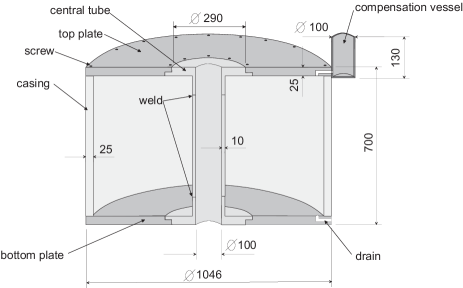
figure

Figure 18: Drawing of the field mass. All dimensions are given in mm.

A cut-away drawing of a FM tank is shown in Fig.18. All pieces were made from stainless steel type No. 1.4301 which is resistant to mercury and has a low magnetic susceptibility. The pieces were sealed to one another with mercury resistant Perbunan O-rings. The top and bottom plates were fastened to the central piece with 12 screws. The top and bottom plates were screwed to the outer casing with 24 screws.

Due to the nearness of the central piece to the TM’s, especially close tolerances were specified for this piece. The central piece was annealed before machining to remove tensions which could deform the piece during machining. A surface roughness value of $<1$ $\mu m$ was obtained by grinding the surface after machining. The roughness value is defined as the average height of the peaks times the area of peaks relative to the total area of the surface.

The top and bottom plates were less critical than the central piece. A surface roughness value of 6 to 10 $\mu$m was specified for the machining of the inner surface of these pieces. The inner surface of the casing was even less critical and a surface roughness value of 15 $\mu$m was specified for it.

Since the mercury was filled into the tanks under vacuum conditions, it filled more or less the exact surface profile (i.e. the region between the grooves caused by machining). The mercury in the filled tank was under positive pressure on all surfaces including the top plate. The over pressure ranged from about 0.1 bar on the top plates (due to the height of mercury in the compensation vessel shown in Fig. 18) and 1 bar on the bottom plates. The bulging of the central cylinder and the outer casing due to the mercury pressure was calculated using the equations for thin cylindrical shells Ti87 . The inward bulging of the central tube was found to have a maximum value of 0.17 $\mu$m which is completely negligible for the present experiment. The maximum outward bulging of the outer casing was approximately 4 $\mu$m and resulted in a small (8 ppm) correction of the volume. The loading of the tanks produced a 2 $\mu$m elongation of the outer casing corresponding to a relative volume increase of 1 ppm.

Before the tanks were assembled, measurements of the individual pieces were made with a coordinate measuring machine (CMM). The inner diameters of the central tube were checked with a special dial gauge and found to agree with the CMM values. The wall thickness of the outer casing, top and bottom plates were measured with a wide jaw micrometer having a dial gauge readout.

Figure 19: Data and fit for the upper surface of the lower tank as a function of radius. The solid curve is the fit function based on the theory of circular plates. The offset has been chosen such that the z-value is 0 mm at a radius of 60 mm.

After the tanks were filled with mercury, measurements of the outer surface of the top and bottom plates were made with a laser-tracker (LT). It was not possible to measure the outer surface of the casing due to the close confines of the pit. The LT measurements were made in the dynamic mode in which the retro reflector is moved on the surface and readings are taken as fast as possible (1000 per s). An example of these data for the top surface of the lower tank is shown in Fig. 19. The data for the other plates are similar. The force due to the mercury loading which tended to stretch the central tube, and to a lesser extent the outer casing, could be determined from these data using equations based on thin axial symmetric plates and shells Ti87 . The force on the central tube was calculated to be ($17\pm 8$ kN) which resulted in an elongation of 15 $\mu$m.

Finally, after the mercury had been removed from the tanks, additional LT measurements were made of the outside height of the central tube in order to clear up a discrepancy of this dimension as measured with the CMM and LT.

The form of the central tube and outer casing as determined by the analysis of the measurements was very nearly circular; however, the deviation from perfect roundness was larger than the expected accuracy of the measurements. For the purpose of determining the actual accuracy of the measurements, a least-squares fit was made to the data employing a number of Fourier terms. The uncertainty of the measured data was then determined by setting the $\chi^{2}$ of this fit equal to the DOF.

For the purpose of determining the uncertainty of the volume and the mass-integration constant, we have employed effective dimensions describing a hollow, right circular cylinder. The effective value of the small radius $r$ and height $h$ of the central piece were assigned the approximate values of 60 mm and 650 mm, respectively. The effective inner radius $R$ of the casing was then determined such that the inside volume of the tank was the value determined from measurements.

Besides the accuracy of the directly measured dimensions, one has also to consider the effect of the expansion coefficient of the stainless steel times the temperature difference between measurement of the piece and the temperature during the gravitational measurement, accuracy of the surface roughness and the deformation due to the load. The accuracy of the temperature, roughness and deformations effects are assumed to be one half of the change caused by these effects. An estimate of these accuracies for the inside effective dimensions of the tanks is given in Table 2.

Table 2: Estimated uncertainty in $\mu m$ of the effective values for the radius $r$ of the central tube, the radius $R$ of the outer casing and the height $h$ of the central tube due to various effects. The uncertainties apply to the inside dimensions of the tank.

Description	$\sigma_{r}$	$\sigma_{R}$	$\sigma_{h}$
measurement	1.0	5	20
thickness	-	-	5
temperature	0.3	4	6
elongation	-	-	7
bulge	0	2	-
roughness	0	6	7
Total	1.1	9	24

IV.3 Weighing the Mercury

After a preliminary measurement in which the tanks were filled with water, the water was drained from the tanks and they were ventilated with warm dry air. The tanks were then evacuated to a pressure of $10^{-2}$ mbar using a rotary pump with an oil filter to prevent back streaming in preparation for being filled with mercury.

Since the tanks were to be filled with mercury only once, every effort was made to weigh the mercury as accurately as possible during the filling. The mercury (specified purity 99.99%) was purchased in 395 flasks each weighing 36.5 kg and containing 34.5 kg of mercury. The general procedure for filling each tank was as follows. The outer surface of the flasks were first cleaned with ethanol. Half of the flasks were brought into a measuring room near the experiment and allowed to come into equilibrium with the room atmosphere for a few days. These flasks were then weighed over a period of one week. Then, one after another, the flasks were attached to the transfer device. Most of the mercury in a flask was transferred via compressed nitrogen, first into an intermediate vessel used as a vacuum lock and then into the evacuated tank. A small amount of mercury was intentionally left in each flask in order not to transfer any of the thin oxide layer floating on the surface. The filling of a tank required one week. After completion of the filling, the flasks with their small remaining mercury content were weighed again. The entire process was then repeated for the second tank.

Various precautions and test measurements were undertaken to insure the accuracy of the weighings. The balance employed for these measurements was type SR 30002 made by Mettler-Toledo. The balance was operated in the differential mode with accurately known (5 mg) standards for weights less than 2 kg (for empty flasks) and a stainless steel mass of approximately 36.6 kg made in our machine shop (for full flasks). The mass of the 36.6 kg weight was calibrated several times at METAS and remained constant within the 18 mg (the certified accuracy of the weighings) during the weighing of the mercury. The reproducibility of the weighing of an almost empty flask or full flask was 20 mg. The average of three weighings was made for empty and full flasks with the balance output transferred directly to a computer via an RS232 interface. The balance was checked for nonlinearity and none was found within the accuracy of the standard weights. A centering table was used which allowed the flasks to be off center by as much as 2 cm without influencing the measurement. Atmospheric data used for buoyancy corrections were taken several times a day. A 10 kg calibration test was made once a day and the balance zero was checked every hour. It was found that the flasks were magnetized along their symmetry axis. Rotating the flask on the balance did not change the measured weight but inverting the flask resulted in a 100 mg difference. Since weighings were always made with the flasks in an upright position, no magnetization error occurred in the difference between full and empty flasks. The variation of the weight for 12 flasks was monitored over a period of 8 weeks. The variation was similar for all 12 flasks and amounted to about 20 mg per flask during the 3 weeks required to weigh the flasks and fill the tank. Mercury droplets which had not reached the tanks and small flakes of paint which had accidentally been removed from the outer surface of the flasks during the transfer process were collected and weighed.

The total uncertainty in the approximately 6760 kg of mercury in each tank was 12 g for the upper tank and 15 g for the lower tank which gives a relative accuracy of 2.2 ppm for the mass of mercury in the tanks. A listing of the various weighing uncertainties is given in Table 3. An estimate of the mercury and flask residue that had not been collected (and the uncertainty of the amount collected) was assumed to be 20% of the amount collected. The pressurizing of the flasks with nitrogen during transfer resulted in a buoyancy correction of the almost empty flasks due to the difference in density between air and nitrogen. The flasks were sealed after use, but air gradually replaced the nitrogen. The assumption of a constant density (approximate equation) for the gas left in each empty flask during the time of the measurement amounted to an uncertainty of 7 and 8 g for the upper and lower tanks, respectively. The change in mass of the flasks during the three week measurements gave an uncertainty of 4 g for each tank. The accuracy of the standard masses caused an uncertainty of 3.7 g for each tank. Air buoyancy uncertainties resulted in an uncertainty of 1.2 g for each tank. The statistical uncertainty due to reproducibility of the balance was 0.4 g for each tank.

Table 3: A listing of the weighing uncertainties for the upper and lower tanks. All uncertainties except that of the standard masses are independent for each tank. The total mass of mercury in each tank was approximately 6760 kg.

Type of Uncertainty	Upper	Lower
	Tank[g]	Tank[g]
loss of mercury and residue from flasks	8	11
approximate equation	7	8
mass variation of flasks	4	4
uncertainty of standard masses	3.7	3.7
buoyancy correction	1.2	1.2
weighing statistics	0.4	0.4
total uncertainty	12	15

IV.4 Mass Distribution of the Central Piece

Although the principle mass making up the FM’s was mercury and therefore had only a negligible density variation due to its pressure gradient, the density variation of the walls of the tanks was important in determining the mass-integration constant. In particular, the two central pieces which were very near to the TM’s and which were composed of three different pieces of stainless steel welded together were critical for this determination. Therefore after the gravitational measurements had been completed, the central pieces were cut into a number of rings in order to determine the density of these rings and thus the mass distribution of the central pieces.

As shown in Fig. 18, each central piece was composed of upper and lower flanges and a central tube. The material of the flanges extended about 40 mm beyond the surface of the flanges in the form of the central tube. In order to determine the vertical mass distribution in the flanges, three rings of 10 mm height were cut from each of these 40 mm sections with the last ring straddling the weld between flange and central tube. The weight and dimensions of the various pieces (12 rings, 4 flanges and two central sections of the tube) were used to determine the densities of these pieces. The densities of the flanges were found to be between 7.9138 to 7.9147 g cm^-3 and the densities of the central section of tubes were 7.9062 and 7.9101 g cm^-3. The accuracy of the absolute-density determinations was somewhat better than 0.001 g cm^-3. The density of the weld regions did not differ significantly from that of the flanges. The variation of the flange densities over the 65 mm of the flange and adjoining section of the tube was found to be less than 0.005 g cm^-3. From these measurements, it was not possible to determine a radial density gradient of the flanges. For calculating the effect of a radial gradient on the mass-integration constant, we shall make the assumption that the radial density variation was less than 0.005 g cm^-3 over the radial dimension of the flange (160 mm). The vertical density gradients of the central tubes were not important since their effects on the gravitational signal are almost completely cancelled due to the symmetry of central tube relative to the apart-together measurements with the FM’s.

IV.5 Using the Measured Dimensions

The first step in calculating the mass-integration constant was to enter the measured dimensions and masses of the various pieces in a computer program. For pieces that had essentially axial symmetry such as the central tube and the outer casing, an average radius was determined from the data measured at each height and used in further calculations. For horizontal surfaces which were nearly planar such as the top and bottom plates, an average height was determined from the data at each measured radius and used in further calculations. Since the original data were normally available only in Cartesian coordinates, it was necessary to determine the symmetry axis and make the conversion to cylindrical coordinates. For data without axial symmetry such as screws, screw holes and linear objects, single or multiple point masses were used. With this reduced set of dimensions, approximately 580 data elements were necessary to describe each tank.

As a preliminary calculation related to the mass-integration constant, the volume of the individual pieces and the inside volume of the tanks were calculated from the reduced dimensions. Using the known weight of the piece, the calculated volume allowed the density of the material to be determined. This was a valuable test to check whether the input data for the piece was reasonable.

The volume for pieces with axial symmetry was determined by making a linear interpolation between the points of the reduced data. The volume of a piece was thus composed of a sum of cylindrical rings with rectangular and right triangular form. A cylindrical ring with circular cross section was used for the volume of O-rings. The accuracy of the linear approximation in the volume determination was checked relative to a quadratic approximation of the surface. The linear approximation was found to be sufficient for all calculations.

The original CMM measurements had been made for 12 $\varphi$ angles at 14 heights on the central tube, at 4 radii on the horizontal surfaces of the central flange, at 11 radii on the horizontal surfaces of the top and bottom plates and at 7 heights on the outer casing. Although many more points of the horizontal surfaces were measured with the LT, they were reduced to the original CMM points for the purpose of volume integration and mass integration by fitting functions to the LT data. Only outside surfaces were measured with the LT. Inside dimensions were obtained from the LT data by subtracting the micrometer-thickness values. The only measurements of the casing radius were the CMM measurements of the inner radius. The outer surface of the casing was determined from the CMM values combined with the micrometer data.

IV.6 Density Constraint

Since the mercury represented roughly 90% of the total tank mass, special attention was given to its contribution to the signal. The density of mercury samples from each tank was measured at the Physikalisch-Technische Bundesanstalt, Braunschweig with an accuracy of 3 ppm. One can use this density and mass measurements of the mercury (see Sec. IV.3) to obtain better values for the effective tank dimensions and thus for the mass-integration constant. This results in a correlation among the effective parameters, $r,R,h,m$. The method employed to determine the best parameters representing the effective values (determined from measurements as described in the previous section) is based on minimizing a $\chi^{2}$ function of the form

$$\chi^{2}= \left(\frac{r-r_{0}}{\sigma_{r}}\right)^{2}+\left(\frac{R-R_{0}}{\sigma_{R}}\right)^{2}+\left(\frac{h-h_{0}}{\sigma_{h}}\right)^{2}$$

$$+\left(\frac{m-m_{0}}{\sigma_{m}}\right)^{2}+\left(\frac{\varrho-\varrho_{0}}{\sigma_{\varrho}}\right)^{2}$$ (3)

subject to the density constraint

$$\varrho=\frac{m}{\pi(R^{2}-r^{2})h}.$$ (4)

After substituting $\varrho$ from Eq. (4) in Eq. (3), $\chi^{2}$ becomes a function of the four parameters $r$, $R$, $h$, $m$, the five measured quantities $r_{0}$, $R_{0}$, $h_{0}$, $m_{0}$, $\varrho_{0}$ and their uncertainties (see Table 4 for the uncertainties of the effective values). The simplex method was used to minimize $\chi^{2}$ and thereby obtain best values for the fit parameters. Although $\varrho$ is not explicitly one of the fit parameters, a best value for $\varrho$ can be obtained by substituting best fit parameters in Eq. (4).

The difference between best fit parameters and the measured values are shown in Table 4 along with the resulting minimum $\chi^{2}$. It is seen that the difference between parameters and measured values is less than the error in all cases and that $\chi^{2}$ is consistent with the expected $\chi^{2}$ for a least-squares fit with one DOF.

Table 4: The correlated measured values, their uncertainties and the difference between the best fit parameters and the measured values for upper and lower tanks labelled 1 and 2. Only approximate values are shown for the measured quantities.

	Measured		Uncertainty		Difference 1		Difference 2
$r_{0}$	60	mm	1.1	$\mu\mbox{m}$	0.007	$\mu\mbox{m}$	0.013	$\mu\mbox{m}$
$R_{0}$	498	mm	9.0	$\mu\mbox{m}$	-3.5	$\mu\mbox{m}$	-7.1	$\mu\mbox{m}$
$h_{0}$	650	mm	24.0	$\mu\mbox{m}$	-9.5	$\mu\mbox{m}$	-19.0	$\mu\mbox{m}$
$m_{0}$	6760	kg	14.8	g	0.3	g	0.7	g
$\varrho_{0}$	13.54	g/cm3	40.6	$\mu\mbox{g/cm}^{3}$	-1.3	$\mu\mbox{g/cm}^{3}$	-2.5	$\mu\mbox{g/cm}^{3}$
$\chi^{2}$					0.27		1.18

In order to obtain the uncertainty of the mass-integration signal one needs the parameter-error matrix involving $r$, $R$, $h$, $m$ and $\varrho$ multiplied by partial derivatives of the signal with respect to the these quantities. The partial derivative with respect to $\varrho$ is zero since it does not occur explicitly in the expression for the signal. The error of the signal $S$ is given by

$$\sigma_{S}=\left(\sum_{i,j}\frac{\partial S}{\partial x_{i}}\frac{\partial S}{\partial x_{j}}\textrm{err}(x_{i},x_{j})\right)^{1/2}$$

where the $x_{i}$ and $x_{j}$ are any pair of the measured quantities and err$(x_{i},x_{j})$ is the 5 by 5 parameter-error matrix. Assuming that, for small variations about the measured values, the fit parameters represented by the 5-dimension vector $\overline{y}$ can be expressed as a linear function of the measured values $\overline{x}$ of the form $\overline{y}=T\overline{x}+\overline{a}$. The parameter-error matrix can be written as

$$\textrm{err}(y_{i},y_{j})=TVT^{t}$$

where T is the Jacobi derivative of $y$ with respect to $x$, $T^{t}$ is its transpose, $V$ is the 5 by 5 matrix covariance matrix (i.e. $V_{i,j}=err(y_{i},y_{j})$) with all zero elements except along its diagonal and $\overline{a}$ is a constant vector. The elements of the matrix $T$ and the vector $\overline{a}$ were determined numerically by solving a system of linear equations in which the fit parameters were determined for measured values incremented by small amounts ($\sigma_{x}$).

The partial derivatives were also determined numerically by calculating the signal for measured values with small increments ($\sigma_{x}$). The signal was calculated using actual dimensions of the deformed tanks corrected by factors relating the $r,R,h$ parameters to the effective dimensions $r_{0},R_{0},h_{0}$. The resulting covariance matrix representing the square of the uncertainty in the calculated mass-integration signal is shown in Table 5. It is seen that the elements involving $R$ and $h$ are much larger than those for $r$ and $m$. For the upper tank (tank 1), the relative uncertainty of the calculated mass-integration constant due to the correlated dimensions is 2.14 ppm. For tank 2, it is 2.41 ppm. The large cancellation occurring in the sum of the elements results in the uncertainty for these constrained parameters being approximately a factor of seven smaller than the uncertainty that would be obtained without the density information.

Table 5: The covariance matrix involving $r,R,h,m$ for the uncertainty of the calculated signal. Values are given in units of ng². Only the upper part of the symmetric matrix is shown. The sum of all element in the full matrix is 2.84 $\mbox{ng}^{2}$. The sum of a similar diagonal matrix for uncorrelated $r,R,h,m$ values (not shown) is 175 $\mbox{ng}^{2}$.

	r	R	h	m
r	$0.52$	$0.04$	$0.05$	$0.0003$
R		$35.77$	$-42.52$	$-0.20$
h			$51.62$	$-0.25$
m				$0.66$

IV.7 The Effect of Air Density

Since air is not present in the region of the FM’s, the motions of the FM’s results in a force on the TM’s due to the mass of the air elsewhere. It is as if there were a negative contribution to the mass of the FM’s due to the lack of air in this region. This effect depends upon the density of the air in the region surrounding the FM’s.

The air pressure, the relative humidity and the air temperature were recorded every 12 min during the gravitational measurement thereby providing the information necessary to determine the air density. The effect of air density on the calculated mass-integration constant was approximately 100 ppm. The variation of the mass-integration constant for this effect was only about 1 ppm. Thus, it was sufficient to employ only the average value of the air density during the entire gravitational measurement. The average density employed was 1.156 $\mbox{kg}/\mbox{m}^{3}$.

IV.8 The Effect of Mercury Expansion

Due to the small temperature variations of the FM’s, the volume of the mercury relative to the volume of the tanks changed slightly during the gravitational measurement. This resulted in a variation of the mercury height in the compensation vessels. The height of the mercury in each compensation vessel was recorded every 12 min during the experiment. The calculated mass-integration constant varied by only 0.3 ppm due to this effect. Therefore, only an average value of the mercury height in each compensation vessel was employed in determining the mass-integration constant for the entire measurement.

IV.9 Uncertainties Affecting the Mass-Integration Constant

The relative uncertainties of the mass-integration constant due to the various measured and estimated quantities relating to either the upper or lower TM or to either the upper or lower FM are given in Table 6. The signs of the estimated quantities have been chosen to give the largest uncertainty of the mass-integration constant. With the exception of the constrained quantities $r$, $R$, $h$, and $m$, all measured quantities of this table are independent (i.e. uncorrelated). All estimated quantities are also independent. The total uncertainty of the mass-integration constant due to the measured quantities listed in Table 6 results in a relative statistical uncertainty of 4.89 ppm. The total uncertainty of the mass-integration constant due to estimated quantities results in a relative systematic uncertainty of 3.25 ppm.

Table 6: Mass-integration constant relative uncertainties (ppm) associated with the measured quantities. ’Upper’ and ’Lower’ refer to the upper and lower FM or TM quantities. The values in parentheses are the uncertainty of the measured quantities. Where two measured values are listed, the first applies to the upper object and the second to the lower object. Quantities marked with a ^∗ are obtained from estimated limiting values. All uncertainties are independent except for the constrained quantities r,R,h,m. However, these constrained quantities are independent for the upper and lower tanks.

Measured Quantity	Upper	Lower
FM Quantities
$r,R,h,m$ constrained	$1.20$	$1.09$
position=2460 or 1042 mm (35 $\mu$m)	$2.05$	$2.99$
inner radius=50 mm (1.1 $\mu$m)	$0.91$	$0.91$
travel=709 mm (10 $\mu$m)	$0.95$	$1.22$
upper plate mass=153 kg (0.9 g)	$0.01$	$0.01$
lower plate mass=154 kg (0.45 g)	$0.02$	$0.02$
central piece mass=46 kg (0.18 g)	$0.03$	$0.03$
outer tube mass=412 kg (0.83 g)	$0.01$	$0.01$
central piece no density gradient	$0.03$	$0.03$
central piece z density gradient∗	$<0.03$	$<0.03$
central piece r density gradient∗	$<1.1$	$<1.1\par$
TM Quantities
radius=23 mm (5 $\mu$m)	$0.57$	$0.57$
height=77 mm (5 $\mu$m)	$0.49$	$0.87$
position=2495, 1077 mm (35 $\mu$m)	$0.45$	$0.32$
mass=1.1 kg (300 $\mu$g)	$0.14$	$0.14$
off center=0.44 or 0.51 mm (0.1 mm)	$1.03$	$1.03$
angle relative to vertical ∗	$<1.85$	$<1.85$
relative z density gradient∗	$<0.9$	$<0.7$
relative r density gradient∗	$<0.02$	$<0.02$

In addition to the uncertainties related to either TM alone, there is the common vertical displacement (shown as $\varepsilon$ in Fig. 17) of both TM’s due to evacuating the system. The uncertainty of this displacement results in a relative uncertainty of the mass-integration constant equal to 0.78 ppm which is added to the other uncertainties as an independent relative uncertainty. Including the uncertainty of $\varepsilon$ results in a relative statistical uncertainty of the mass-integration constant equal to 4.95 ppm.

V Discussion of Measurements

The measured gravitational signal discussed in Secs. III.7 to III.11 is 784,883.3(12.2)(5.8) ng. The calculated mass-integration constant determined in Secs. IV.1 to IV.5 is 784,687.8(3.9)(2.6) ng. Using these values, we obtain the value for the gravitational constant

$G$=6.674252(109)(54)$\times 10^{-11}\;\mbox{m}^{3}\;\mbox{kg}^{-1}\;\mbox{s}^{-2}$.

A summary of the relative uncertainties contributing to this result is given in Table 7.

Table 7: Relative statistical and systematic uncertainties of $G$ as determined in this experiment.

Description	Statistical(ppm)	Systematic(ppm)
Measured Signal
Weighings	11.6
TM-sorption	7.4	7.4
Linearity	6.1
Calibration	4.0	0.5
Mass Integration	5.0	3.3
Total	16.3	8.1

The relative statistical and systematic uncertainties of this result are 16.3 ppm and 8.1 ppm, respectively. The two largest contributions to the total relative uncertainty are the statistical uncertainty of the weighings (11.6 ppm) and the combined statistical and systematic uncertainty due to the TM-sorption effect (10.3 ppm). All uncertainties have been given as one sigma uncertainties. Statistical and systematic uncertainties have been combined to give a total uncertainty by taking the square root of the sum of their squares.

V.1 Comparison with Our Previous Analysis

Our previously published value Sa02 for $G$ was $6.674070(220)\times 10^{-11}\;\mbox{m}^{3}\;\mbox{kg}^{-1}\;\mbox{s}^{-2}$ which was based on the measurements of both the copper and tantalum TM’s. The value for the copper TM’s alone was $6.674040(210)\times 10^{-11}\;\mbox{m}^{3}\;\mbox{kg}^{-1}\;\mbox{s}^{-2}$. The value obtained for $G$ in the present analysis for only the copper TM’s ($6.674252((124)\times 10^{-11}\;\mbox{m}^{3}\;\mbox{kg}^{-1}\;\mbox{s}^{-2}$) is in reasonable agreement with the previous value. The difference between the present and previous result is due primarily to the correction for the ZP curvature which was not taken into account in the previous analysis. A minor difference is also due to a slightly different selection of the analyzed data.

The uncertainty given for the present result is appreciably smaller than that of our previous result. This is due to a better method used in computing the nonlinearity correction (Sec. III.10) and a calculation of the mass-integration constant (Sec. IV.5) using the mercury density as a constraint. The uncertainty of the linearity correction was reduced from 18 ppm to 6.1 ppm and the uncertainty of the mass-integration constant was reduced from 20.6 ppm to 6.7 ppm. The statistical uncertainty of the weighings in the present analysis is somewhat larger than the previous value (9.1 ng vs 5.4 ng). This is due to the correlation of the ZP-corrected data of the present analysis. The previous ABA analysis involved only uncorrelated data.

V.2 Comparison with Other Measurements

Recent measurements Gu00 ; Qu01 ; Ar03 of the gravitational constant with relative errors less than 50 ppm are listed in Table 8 and shown in Fig. 20. We list only the latest publication of each group. It is seen that the present result is in good agreement with those of Gundlach and Merkowitz Gu00 and Fitzgerald Ar03 . It is in disagreement (3.6 times the sum of the uncertainties) with the result of Quinn et al. Qu01 .

Figure 20: Plot of recent measurements with relative errors less than 50 ppm

All of the measurements listed in Table 8 with the exception of our own were performed using torsion balances. It is therefore instructive to compare the problems encountered in the different types of measurements.

In the measurements being discussed, the statistical accuracy in determining the gravitational signal was obtained in measurements lasting one to six weeks. However, as in the case of all precision measurements, the time required for obtaining a good statistical accuracy of the measurement is less than the time required to obtain calibration accuracy of the equipment and the time necessary to investigate and eliminate systematic errors. All of the measurements listed in Table 8 have been long, on-going investigations which have lasted for periods up to ten years.

Although the beam-balance measurement was made with more massive FM’s (15 t) than were employed in the torsion-balance measurements ($<60$ kg), the larger gravitational signal had to be measured in the presence of the TM weight. In our experiment the gravitational signal was roughly 0.7 ppm of the total weight on the balance. This small ratio of signal to total weight on the balance resulted in larger effects of zero-point drift as well as larger statistical noise in the beam-balance data than in the torsion-balance data. In the torsion-balance measurements, the deflection of the balance arm is due entirely to the gravitational force to be determined with only small perturbations from distant moving objects.

A similar problem has to do with the change of TM weight that is produced by an adsorbed water layer. In our measurement, this varied with the temperature of the vacuum tube produced by the FM motion. This resulted in one of the largest contribution to the uncertainty of the gravitational signal (see Sec. III.10). In the beam-balance measurement the weight change adds directly to the signal whereas in the torsion-balance it adds only to the mass of the torsion-arm and is therefore a negligible effect.

The calibration of the beam balance, while simple in principle, is difficult in practice due to the lack of calibration masses having the required mass and accuracy. We have used an averaging method to correct for the nonlinearity of the balance (see Sec. III.11) involving a large number of auxiliary masses. This allowed the comparison of the gravitational signal with a heavier, accurately known calibration mass. The accurate calibration of the torsion balance also presents a problem. Various methods involving either electric forces or an angular acceleration of the measuring table to compensate the gravitational force have been used.

In our measurement, the TM was positioned at a double extremum of the force field produced by the FM’s. This greatly reduces the relative accuracy of the distance measurements required to determine the mass-integration constant. It also reduces the problem resulting from a density gradient in the TM. It is difficult to compare the problems involved in determining the mass-integration constant for the two types of experiments. It appears that the distance between the field masses attracting the small mass of the torsion balance must be measured with very high absolute accuracy (1 $\mu$m  is the accuracy given for this distance in the torsion balance experiments).

The use of liquid mercury as the principle component of the FM’s reduces the problem associated with the density gradients of the FM’s. There is still the density gradient of the vessel walls which has to be considered. The field masses employed in the torsion-balance experiments were either spheres or cylinders. The FM’s were rotated between measurements in order to compensate gradient effects.

The large mercury mass resulted in deformations of the vessel which had to be accurately determined. The FM’s although, nearly cylindrical in form, required more than 1000 ring and point-mass elements in order to determine the mass-integration constant. A similar problem (but on a smaller scale) occurs in the torsion experiments in accounting for small imperfections of the spheres, cylinders or plates and in determining their relative positions.

The determination of $G$ using a beam balance is beset with a number of problems which we have tried to describe in detail. We have been able to reduce the uncertainty in $G$ resulting from these problems to values comparable to the statistical reproducibility of the weighings determining the gravitational signal. The total uncertainty for $G$ which we obtain with a beam balance is comparable to the uncertainty quoted in recent torsion-balance determinations of $G$. We believe that the beam-balance measurement involving a number of quite different problems than encountered in torsion balance measurements can therefore provide a useful contribution to the accuracy of the gravitational constant.

Table 8: Recent measurements of the gravitational constant. Statistical and systematic uncertainties have been added as if the were independent quantities.

Reference	$G[10^{-11}\;\mbox{m}^{3}\;\mbox{kg}^{-1}\;\mbox{s}^{-2}]$
Gundlach and Merkowitz Gu00	6.674215( 92)
Quinn et al.Qu01	6.675590(270)
Armstrong and Fitzgerald Ar03	6.673870(270)
Present analysis	6.674252(124)

VI Acknowledgements

The present research has been generously supported by the Swiss National Fund, the Kanton of Zürich, and assistantship grants provided by Dr. Tomalla Foundation for which we are very grateful. The experiment could not have been carried out without the close support of the Mettler-Toledo company which donated the balance for this measurement and made their laboratory available for our use. We are also extremely grateful to the Paul Scherrer Institut for providing a suitable measuring room and the help of their staff in determining the geometry of our experiment. We also wish to thank the Swiss Metrological Institute and the Physikalisch-Technische Bundesanstalt, Braunschweig, Germany for making a number of certified precision measurements for us. Our heartfelt thanks are also extended to the staff of our machine shop for their advice and precision work in producing many of the pieces for this experiment. We wish to thank E. Klingelé for determining the value of local gravity at the measuring site. We are also indebted to the firms Almaden Co., Metrotec A.G. and Reishauer A.G. for the services they provided.

VII Appendix

The general idea in determining the $z$ component of force on a small volume element of a TM is first to calculate the potential along the $z$ axis due to the FM. The off-axis potential can then be obtained by making a Taylor series expansion for small $r$ and substituting this in the Laplace equation. This is the procedure which is often used in electrostatic calculations Gl56 . The force in the $z$ direction is just the negative derivative of this potential with respect to $z$. We present first a derivation of the force for the axially symmetric case and then describe the modification required for a nonaxially symmetric potential.

The gravitational potential on the $z$ axis of a homogeneous, torus of rectangular cross section with density $\varrho_{FM}$, inner radius $R_{1}$, outer radius $R_{2}$ and half height $Z$ is given by the equation

$$\Phi(r=0,z)=2\pi\varrho_{FM}G\int_{-Z/2}^{Z/2}\int_{R1}^{R2}\frac{r^{\prime}dr^{\prime}\;dz^{\prime}}{\sqrt{{r^{\prime}}^{2}+(z^{\prime}-z)^{2}}}$$ (5)

where $r$ and $z$ are the radial and axial coordinates of a point within the TM expressed in cylindrical polar coordinates. For convenience, one chooses the zero of the potential at the center of mass of a TM. For simplicity, the cross section of the FM employed in Eq. 5 has been chosen to be a rectangle. Besides the torus with rectangular cross section, analytic expressions for the two dimensional integrals with triangular and circular cross sections were also employed.

The potential at points close to the axis can be calculated as a power series in $r$

$$\Phi(r,z)=a_{0}+a_{1}r+a_{2}r^{2}+a_{3}r^{3}+\ldots=\sum_{i=0}^{\infty}a_{i}r^{i}\;$$ (6)

with unknown coefficients $a_{1}$,$a_{2}$,$\ldots$ which are functions of $z$ alone. For $r$=0, one has $a_{0}=\Phi(0,z)$. The gravitational field satisfies the Laplace equation $\nabla^{2}\Phi=0$. Applying the Laplace operator in cylindrical coordinates to Eq. 6 leads to

$$\nabla^{2}\Phi=a_{1}r^{-1}+\sum_{i=0}^{\infty}r^{i}\left(\frac{d^{2}a_{i}}{dz^{2}}+\left(i+2\right)^{2}a_{i+2}\right)=0\;.$$

This equation is valid for all $r$. Since $\nabla^{2}\Phi=0$ for $r=0$, $a_{1}$ must be identically zero. Thus, the values for $a_{i}$ can be calculated recursively from

$$a_{i+2}=-\frac{1}{\left(i+2\right)^{2}}\frac{d^{2}a_{i}}{dz^{2}}$$

starting with either $a_{0}$ or $a_{1}$. Since $a_{1}=0$, all terms with odd $i$ are zero and $a_{i}$ for even $i$ can be obtained starting with $a_{0}$. By induction, it is easily shown that the coefficient $a_{2n}$ is

$$a_{2n}=\left(-\frac{1}{4}\right)^{n}\frac{1}{\left(n!\right)^{2}}V^{(2n)}(z)$$

with

$$V^{(2n)}(z)=\frac{d^{2n}\Phi(0,z)}{dz^{2n}}.$$

Here, $V^{(0)}$ is just $\Phi(0,z)$ which can be easily calculated using Eq. 5.

Using this expression for the coefficients in the expansion 6, the gravitational potential can be calculated from the sum

$$\Phi(r,z)=\sum_{i=0}^{\infty}\left(-\frac{1}{4}\right)^{i}\frac{1}{\left(i!\right)^{2}}V^{(2i)}(z)\;r^{2i}\;.$$ (7)

The gravitational field $g_{z}$ in z-direction is given by $-\partial\Phi/\partial z$ or

$$g_{z}(r,z)=-\sum_{i=0}^{\infty}\left(-\frac{1}{4}\right)^{i}\frac{1}{\left(i!\right)^{2}}V^{(2i+1)}(z)\;r^{2i}\;.$$

Integrating $g_{z}$ over the volume of the TM, one obtains the force on the TM in the $z$ direction

$$F_{z}=-2\pi\varrho_{TM}\times$$

$$\sum_{i=0}^{\infty}\left(-\frac{1}{4}\right)^{i}\frac{1}{\left(i!\right)^{2}}\int_{-b}^{+b}\ dz^{\prime}\int_{0}^{r}V^{(2i+1)}(z)\;r^{\prime 2i}r^{\prime}\ dr^{\prime}\;$$ (8)

where the origin has been taken to be the center of the TM. The integration over $r$ is trivial. The integration over $z$ is

$$\int_{-b}^{+b}V^{(2i+1)}dz^{\prime}=V^{(2i)}(b)-V^{(2i)}(-b)\;.$$

Making a Taylor expansion for small $b$ on the right side of equation, one obtains

$$\int_{-b}^{+b}V^{(2i+1)}dz^{\prime}=$$

$$V^{(2i)}(0)+bV^{(2i+1)}(0)+\frac{1}{2!}b^{2}V^{(2i+2)}(0)+\ldots$$

$$-V^{(2i)}(0)+bV^{(2i+1)}(0)-\frac{1}{2!}b^{2}V^{(2i+2)}(0)+\ldots\;.$$

Adding similar terms results in

$$\int_{-b}^{+b}V^{(2i+1)}dz^{\prime}= 2bV^{(2i+1)}(0)+\frac{2}{3!}b^{3}V^{(2i+3)}(0)$$

$$+\frac{2}{5!}b^{5}V^{(2i+5)}(0)+\ldots$$

or

$$\int_{-b}^{+b}V^{(2i+1)}dz^{\prime}=\sum_{j=0}^{\infty}\frac{2}{(2j+1)!}b^{2j+1}V^{(2i+2j+1)}(0)\;.$$ (9)

The final equation for the gravitational force on a cylinder can then be calculated by combining Eq. 8 and 9 to obtain

$$F_{z}=-2\pi br^{2}\varrho_{TM}\sum_{n=0}^{\infty}V^{(2n+1)}(0)\times$$

$$\sum_{i=0}^{n}\frac{1}{\left(-4\right)^{i}}\frac{1}{i!\left(i+1\right)!}\frac{1}{\left(2n-2i+1\right)!}b^{2n-2i}r^{2i}\ .$$ (10)

Only odd derivatives of the potential are required for this case involving complete axial symmetry. The convergence of the series can be improved by dividing the TM into two or more shorter cylinders. The algebraic expressions for the $V^{2n}(0)$, as determined using ”automatic differentiation” Ra81 , are very long and will not be given here.

The above derivation has assumed that the TM and FM have a common axis of cylindrical symmetry. We will now show how essentially the same equations can be employed for an arbitrary FM potential. This allows one to calculate the potential of a FM with cylindrical symmetry but with its axis displaced and/or tilted relative to that of the TM.

Again, in order to facilitate integration over the volume of the cylindrical TM, one employs cylindrical polar coordinates with the $z$ axis along the symmetry axis of the TM. The potential is now a potential of the form $\psi(x,y,z)=\psi\left(r\cos(\varphi),r\sin(\varphi),z\right)$ which satisfies $\nabla^{2}\psi=0$. The center of mass of the TM is chosen as the zero of potential.

One defines a function $\Psi(r,z)$ such that

$$\Psi(r,z)=(2\pi)^{-1}\int_{\varphi=0}^{2\pi}\psi(r,\varphi,z)d\varphi.$$ (11)

One can then show that this function satisfies the same assumption that were made for the function $\Phi(r,z)$, namely that $\Psi$ has axial symmetry, that it is zero on the $z$ axis and that its Laplacian is zero. It can therefore be used in the Eqs. 7 through 10 instead of $\Phi$ to obtain the gravitational force integrated over the TM.

The axial symmetry of $\Psi$ is obvious since $\varphi$ has been removed by the integration over $\varphi$. The zero potential was chosen to be at the TM center of mass. The Laplacian of $\Psi$ can be shown to be zero by allowing the Laplacian to operate on $\Psi$ as defined in Eq. 11. Reversing the integration and differentiation operations one obtains

$$\nabla^{2}\Psi(r,z)=(2\pi)^{-1}\int_{\varphi=0}^{2\pi}(\nabla^{2}\psi-r^{-2}\frac{\partial^{2}\psi}{\partial\varphi^{2}})d\varphi.$$

The Laplacian of $\psi(r,\varphi,z)$ is zero for an inverse $r$ potential. The integral of the second term is $r^{-2}\partial\psi/\partial\varphi$ evaluated at $\varphi=0$ and $2\pi$ which is also zero. Thus, one obtains the desired result that $\nabla^{2}\Psi(r,z)=0$.

In order to use this property of a potential which does not have axial symmetry about the TM axis (the $z$ axis), one must determine the potential and its derivative with respect to $z$ along the $z$ axis. This is not difficult for the case of a FM which has axial symmetry about an axis not coincident with the TM axis. One merely uses Eq. 7 to determine the potential at radial distances from the FM axis corresponding to points on the TM axis. The force in the $z$ direction (TM axis) is then determined as before using Eqs. 8 and 10. This procedure is particularly useful for the case of TM and FM axes which are parallel but which are displaced relative to one another.

In principle, one can determine the derivatives with respect to $r$ which are required for the force on a TM tilted relative to the vertical; however, in this case it is simpler to approximate the TM by a number of thin slabs displaced from the vertical axis. This completes the discussion of nonaxial-symmetric potentials.

References

- (1) P. J. Mohr and B. N. Taylor, Rev. Mod. Phys. 77, 1(2005).
- (2) E. Fischbach, D. Sudarsky, A. Szafer, C. Talmadge and S. H. Aronson, Phys. Rev. Lett. 56, 3(1986) [Erratum-ibid. 56, 1427(1986)].
- (3) A. Cornaz, B. Hubler and W. Kündig, Phys. Rev. Lett. 72, 1152(1994).
- (4) B. Hubler, A. Cornaz and W. Kündig, Phys. Rev. D51, 4005(1995).
- (5) G. I. Moore, F. D. Stacey, G. J. Tuck, B. D. Goodwin, N. P. Linthorne, M. A. Barton, D. M. Reid and G. D. Agnew, Phys. Rev. D38, 1023(1988).
- (6) C. C. Speake and G. T. Gillies, Proc. R. Soc. London A414, 415(1987).
- (7) J. Schurr, F. Nolting and W. Kündig, Phys. Lett. A248, 295(1998).
- (8) J. Schurr, F. Nolting and W. Kündig, Phys. Rev. Lett. 80, 1142(1998).
- (9) F. Nolting, PhD Thesis, University of Zurich(1998).
- (10) F. Nolting, J. Schurr, St. Schlamminger and W. Kündig, IEEE Trans. Instrum. Meas. 48, 245(1999).
- (11) F. Nolting, J. Schurr, St. Schlamminger and W. Kündig, Meas. Sci. Technol. 10, 487(1999).
- (12) St. Schlamminger, E. Holzschuh and W. Kündig, Phys. Rev. Lett. 89,161102-1(2002).
- (13) St. Schlamminger, PhD Thesis, University of Zurich(2002).
- (14) A. H. Slocum, Precision Eng. 10(2), 85(1988).
- (15) J. E. Furse, J. Phys., E:Sci. Instrum. 14, 264(1982).
- (16) R. Schwartz, Metrologia, 31, 117(1994).
- (17) R. Schwartz, Metrologia, 31, 129(1994).
- (18) A. Reichmuth, Non-Linearity in Mass Comparison. Proc. Intl. Conf. Metrology, Jerusalem (II), pages 58-66, May(2000).
- (19) R. J. Barlow, Statistics, John Wiley and Sons, Chichester(1989).
- (20) W. Glaser, Encyclopedia of Physics, Volume XXXIII, Springer-Verlag, Berlin-Göttingen-Heidelberg(1956).
- (21) S. P. Timoshenko and S. Woinowsky-Krieger, Theory of Plates and Shells, McGraw-Hill, New York(1987).
- (22) L. B. Rall, Lecture Notes in Computer Science 120: Automatic Differentiation: Techniques and Applications, edited by G. Goos and J. Hartmanis, Springer-Verlag, New York(1981) Publishers, Amsterdam(1989).
- (23) J. H. Gundlach and S. M. Merkowitz, Phys. Rev. Lett. 85, 2869 (2000).
- (24) T. J. Quinn, C. C. Speake, S. J. Richman, R. S. Davis and A. Picard, Phys. Rev. Lett. 87, 111101-4(2001).
- (25) T. R. Armstrong and M. P. Fitzgerald, Phys. Rev. Lett. 91, 201101-4(2003).