Odd-parity perturbations of self-similar Vaidya space-time.

Abstract

We carry out an analytic study of odd-parity perturbations of the self-similar Vaidya space-times that admit a naked singularity. It is found that an initially finite perturbation remains finite at the Cauchy horizon. This holds not only for the gauge invariant metric and matter perturbation, but also for all the gauge invariant perturbed Weyl curvature scalars, including the gravitational radiation scalars. In each case, ‘finiteness’ refers to Sobolev norms of scalar quantities on naturally occurring spacelike hypersurfaces, as well as pointwise values of these quantities.

1 Introduction and summary: naked singularities in self-similar collapse.

In the standard picture of gravitational collapse, the implosion that results from the instability of the collapsing object leads to the formation of a black hole horizon prior to the formation of the inevitable singularity [1]. However, it is known that models exist where the ‘horizon before singularity’ order is not followed, and the singularity that results is visible to external observers. There are different reasons why the existence of such naked singularities are an undesirable feature of spacetime: on a fundamental level, they are accompanied by Cauchy horizons leading to a breakdown in predictability of physical laws. On a physical level, the possibility arises that naked singularities may be the source of infinite (destructive) amounts of energy. The Cosmic Censorship Hypothesis (CCH) of Penrose seeks to guard against naked singularities. In rough terms, this hypothesis asserts that naked singularities cannot form in realistic gravitational collapse (there are rigorous mathematical formulations of the hypothesis; see for example [2]). Thus those models which give rise to naked singularities must be unrealistic in some way. Nevertheless, models admitting naked singularities provide probes of the CCH, and studies of naked singularities have influenced the development of exact statements of the hypothesis. There is also some hope that studies of spacetimes admitting naked singularities will shed light on how a general proof of the hypothesis might arise. Of course one must also keep in mind the possibility that such a model cannot be ruled out, and that naked singularities must be considered to be genuine astrophysical objects.

There are at least three ways in which spacetime models admitting naked singularities can be ruled out as providing genuine counterexamples to the CCH. First, the matter model used may be considered to be inappropriate to the description of gravitational collapse on the smallest scale. This is understood to be the case, for example, in fluid models: the singularities that result are ascribed to a breakdown of the matter model rather than a gravitational pathology [3]. Indeed careful statements of the hypothesis insist that the matter model used must be such that it does not develop singularities in flat spacetime [2].

The second way is to demonstrate that the model that includes a naked singularity is unstable in the following way. One shows that a small perturbation of the initial data for the spacetime gives rise to a spacetime that does not admit a naked singularity. This approach has been used by Christodoulou to show that naked singularities forming in the self-similar collapse of a spherically symmetric massless scalar field are unstable [4].

Finally, one looks for instability of the Cauchy horizon associated with the naked singularity. In this scenario, the model admitting a naked singularity is a non-generic member of a class of spacetimes which instead give rise to a null singularity marking the end of the spacetime rather than a problematic horizon. This situation holds a the inner (Cauchy) horizon of charged or rotating black holes [5].

In this paper, we deal with a 1-parameter family of spherically symmetric self-similar spacetimes that admit a naked singularity: the self-similar Vaidya spacetimes. We will study stability of the associated Cauchy horizon.

The question of whether or not these spacetimes provide a serious challenge to the CCH can be answered immediately in the negative. The matter model is null dust, which always forms singularities in flat spacetime. However, there are many classes of spherically symmetric self-similar spacetimes admitting naked singularities that cannot be ruled out on this basis. By studying stability of the Cauchy horizon of Vaidya spacetime, we will provide a template for the study of the same issue in more realistic spacetimes (e.g. self-similar Lemaître-Tolman-Bondi, perfect fluids, Einstein-Klein-Gordon, Einstein-$SU(2)$). There are also other reasons for studying perturbations of Vaidya spacetime. This spacetime is used to model the late stages of stellar collapse in which radiative emission dominates. Studying stability of the spacetime provides information with regard to the effectiveness of this model.

A spacetime is said to be self-similar if it admits a homothetic Killing vector field, i.e. a vector field $\vec{X}$ satisfying

$${\cal{L}}_{\vec{X}}g_{ab}=2g_{ab}.$$

(The choice of non-zero constant on the right hand side is arbitrary, and it should be noted that some authors would refer to $\vec{X}$ as defined here as a proper homothetic Killing vector field, or to the associated symmetry as type-1 self-similarity.) See [6] for an overview of the important role of self-similarity in General Relativity.

The line element of a spherically symmetric spacetime $(M,g)$ can always be written in the form

$$ds^{2}=2F(v,r)e^{P(v,r)}dv^{2}+2e^{P(v,r)}dvdr+r^{2}d\Omega^{2},$$ (1)

where $d\Omega^{2}$ is the standard line element on the unit 2-sphere. The coordinate $v$ is an advanced Bondi coordinate. Taking this null coordinate to increase into the future, it labels past null cones of the axis $r=0$. The line element above maintains its form under the relabelling $v\to V(v)$. Self-similarity holds if and only if $F(v,r)=G(t)$ and $P(v,r)=\psi(t)$ for some functions $G,\psi$ and where $t=\frac{v}{r}$:

$$ds^{2}=-2G(t)e^{\psi(t)}dv^{2}+2e^{\psi(t)}dvdr+r^{2}d\Omega^{2}.$$ (2)

The homothetic Killing vector field is $\vec{X}=v\frac{\partial}{\partial v}+r\frac{\partial}{\partial r}$.

We will use the coordinates $t=v/r$ and a rescaled radial coordinate $x$ defined by $r=e^{x}$. Then the line element reads

$$ds^{2}=e^{2x}\left\{-2Ge^{\psi}dt^{2}+2e^{\psi}(1-2tG)dtdx+2te^{\psi}(1-tG)dx^{2}+d\Omega^{2}\right\}.$$ (3)

A general description of spherically symmetric spacetimes modelling gravitational collapse has been given in [7] and [8]. This can be done without specifying the matter model. Here, we restrict ourselves to the following crucial points, proven in [7]. The second result gives necessary and sufficient conditions for the singularity that necessarily forms at $(v,r)=(0,0)$ to be naked.

Proposition 1

The surface $t=t_{c}$ constant is spacelike (respectively, null, timelike) if and only if $t_{c}(1-t_{c}G(t_{c}))>0$ (respectively, $=0,<0$).

This gives rise to the moniker ‘similarity horizon’ for null hypersurfaces of the form $t=t_{c}$.

Proposition 2

Suppose that the spacetime $(M,g)$ with line element (2)

• satisfies the Einstein equation;

• has energy-momentum tensor satisfying the null energy condition;

• is regular to the past of the scaling origin ${\cal{O}}=(v,r)=(0,0)$, where $v$ is scaled to measure proper time on the regular axis $\{v<0,r=0\}$.

Then there exists a future-pointing outgoing radial null geodesic with past endpoint on ${\cal{O}}$ if and only if there is a positive solution of the equation $1-tG(t)=0$. Furthermore, if $t_{1}$ is the smallest such positive root, then the surface $t=t_{1}$ is the Cauchy horizon of the spacetime.  

We have not defined ‘regularity to the past of ${\cal{O}}$’; it suffices to note that this is a well-defined concept, including limiting behaviour of the metric at the regular axis and the absence of trapped surfaces in $v<0$. Note also that we can characterise the Cauchy horizon as being the first similarity horizon to the future of the scaling origin. The past null cone of the scaling origin is a similarity horizon given by $t=0$.

In the following section, we describe the geometry of Vaidya spacetime, the subject of our analysis, concentrating on the self-similar case. In Section 3, we describe the gauge-invariant approach to perturbations of spherically symmetric spacetimes given by Gerlach and Sengupta [9]. We show that for odd-parity perturbations (see below), the matter perturbation is completely and explicitly determined by an initial data function $\mu_{0}$. The remaining perturbation quantities are determined through a single gauge-invariant scalar $\Pi$, which satisifies an inhomogeneous wave equation with source term depending on $\mu_{0}$. We give existence and uniqueness results, and show that, subject to the specification of regular initial data on a slice $t=t_{i}\in(0,t_{1})$, the function $\Pi$ and its first partial derivatives remain finite up to and at the Cauchy horizon $t=t_{1}$. Thus there is no instability at the level of the metric or the matter perturbation. There remains the possibility that instability is present at the level of the conformal curvature tensor (Weyl tensor) - cf. the mass inflation scenario inside charged spherical black holes [10]. This is ruled out in Section 4 where we show that all the gauge and tetrad invariant perturbed (Newman-Penrose) Weyl scalars remain finite at the Cauchy horizon. Perturbations with angular mode number $l=1$ require a separate (much shorter) treament, which is carried out in Section 5 and yields the same results. We make some concluding comments in Section 6. We note that the analysis of the inhomogeneous wave equation below follows closely our previous analysis of the minimally coupled massless scalar wave equation in a general spherical self-similar spacetime [8]. We use the conventions of [2], and set $G=c=1$.

2 Geometry of Vaidya Spacetime

The Vaidya spacetime metric is the unique solution of the Einstein equations subject to the assumptions that (a) spacetime is spherically symmetric and (b) the energy-momentum tensor is that of null dust, with the dust flow vector $\bar{k}^{a}$ normal to the $SO(3)$ symmetry group orbits (the bar indicates a background quantity). Local conservation of the energy momentum tensor shows that $\bar{k}^{a}$ is geodesic and hypersurface orthogonal, and so one can introduce a null coordinate $v$ with $\bar{k}_{a}=-\nabla_{a}v$, where we assume that $v$ increases into the future. The hypersurfaces $v=$ constant are either future null cones of the axis $\{r=0\}$, coresponding to expanding matter, or past null cones of the axis, corresponding to collapsing matter. We assume the latter (and so conform with the notation of the previous section). Taking as the remaining coordinates the standard angular coordinates $(\theta,\varphi)$ on the unit sphere and the areal radius $r$, the line element can be shown to take the form

$$ds^{2}=-(1-\frac{2m(v)}{r})dv^{2}+2dvdr+r^{2}d\Omega^{2},$$ (4)

where $d\Omega^{2}=d\theta^{2}+\sin^{2}\theta d\varphi^{2}$ is the standard line element on the unit sphere. The energy-stress-momentum tensor is obtained from $8\pi t_{ab}=\bar{\rho}\bar{k}_{a}\bar{k}_{b},$ with $\bar{\rho}=2m^{\prime}(v)/r^{2}$. Then the strong, weak and dominant energy conditions are all equivalent to $m^{\prime}(v)\geq 0$ for all $v$ in the domain of $m$. The line element above is used to model the gravitational collapse of a thick shell of null dust (or a photon fluid) with the choice

$$m(v)=\left\{\begin{array}[]{cc}0&v<0;\\ M(v)&0\leq v<v_{1};\\ M(v_{1})&v_{1}\leq v,\end{array}\right.$$

where $v\to M(v)$ is an increasing $C^{1}$ function on $[0,v_{1})$ and $v_{1}>0$ is arbitrary. Note then that spacetime is a portion of Minkowski spacetime to the past of the past null cone $\{v=0\}$, and is a portion of the Schwarzschild-Kruskal space-time with mass parameter $M(v_{1})$ to the future of the past null cone $\{v=v_{1}\}$. The null fluid is confined to the region $\{0<v<v_{1}\}$, and collapses from past null infinity to form a singularity at $r=0$. The portion of the singularity in $v>0$ is future space-like, but the singular origin $\{(v,r)=(0,0)\}$ may be visible (timelike or ingoing null), depending on the details of the function $M$ at $v=0$. See Figures 1 and 2.

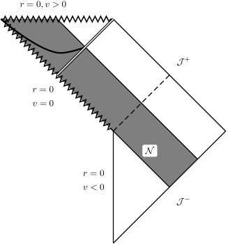
Figure 1: Conformal diagram for Vaidya-Schwarzschild collapse to a globally naked singularity. We use the advanced Bondi co-ordinates $v$ and $r$ described in the text. The Cauchy horizon is shown dashed, the event horizon as a double line and the apparent horizon as a bold curve. Note that the apparent horizon in the matter filled region meets the event horizon at the surface of the ‘star’. ${\cal{N}}$ is the past null cone of the scaling origin. In Figures 1-3, the matter filled region is shaded.

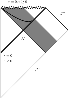
Figure 2: Conformal diagram for Vaidya-Schwarzschild collapse to a black hole. As in Figure 1, the apparent horizon (bold) in the matter filled region necessarily meets the event horizon (double line).

In fact, we will not impose the cut off at $v=v_{1}$, and will take the exterior region $v>0$ to be filled with null dust. That is, we take

$$m(v)=\left\{\begin{array}[]{cc}0&v<0;\\ M(v)&0\leq v.\end{array}\right.$$

We wish to study the stability of the Cauchy horizon in the case when a naked singularity is present. In the cut-off spacetime, the portion of the Cauchy horizon that resides in the Schwarzschild-Kruskal region is (a portion of) a regular outgoing null hypersurface of that spacetime where no singular behaviour can be expected, unless divergence is mediated along the earlier portion of the horizon that resides in the matter-filled region. Thus we are only interested in the matter-filled region of the spacetime, and the cut-off is unnecessary. So our concern is the spacetime of Figure 3.

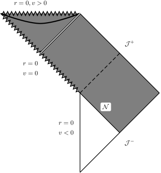
Figure 3: Conformal diagram for Vaidya collapse to a globally naked singularity. The region to the future of $v=0$ is filled with null dust.

This spacetime is self-similar when (and only when) $M$ is a linear function of $v$: $M(v)=\lambda v$ for $\lambda>0$. The restriction on the range of $\lambda$ ensures that the energy conditions are satisfied, and that the trivial case is avoided ($\lambda=0$ corresponds to flat spacetime). Applying Proposition 2, it is then straightforward to show that the singular origin is naked if and only if $\lambda\in(0,\frac{1}{16})$, and we will assume henceforth that $\lambda$ lies in this range.

Introducing the coordinates $t=v/r,x=\log r$ of Section 1, the line element (4) becomes

$$ds^{2}=e^{2x}[-(1-2\lambda t)dt^{2}+2(1-t+2\lambda t^{2})dtdx+t(2-t+2\lambda t^{2})dx^{2}+d\Omega^{2}].$$ (5)

The Cauchy horizon is given by

$$t=t_{1}:=\frac{1-\nu}{4\lambda},$$

and the second future similarity horizon is given by

$$t=t_{2}:=\frac{1+\nu}{4\lambda},$$

where $\nu=\sqrt{1-16\lambda}$. There are no other future similarity horizons. The apparent horizon is spacelike and is located at $t=t_{3}:=1/2\lambda$. This forms to the future of both future similarity horizons: $t_{3}>t_{2}>t_{1}$.

For the calculation of the gauge invariant perturbed Weyl curvature scalars, it will be essential to have an appropriate representation of the radial null directions of self-similar Vaidya spacetime, along with the associated null coordinates. The advanced null coordinate is $v=tr=te^{x}$, so that $v=$ constant describes a past null cone of the axis $\{r=0\}$. The future null cones are described by $u=$ constant, where the retarded null coordinate $u$ is given by

$$u=-e^{x}|t_{1}-t|^{\lambda_{1}}|t_{2}-t|^{\lambda_{2}},$$ (6)

with

$$\lambda_{1}=\frac{\nu+1}{2\nu},\quad\lambda_{2}=\frac{\nu-1}{2\nu}.$$

The region of spacetime with which we will be concerned is that bounded by past and future null infinity, the past null cone of the scaling origin ${\cal{N}}={\cal{H}}^{-}$ and the Cauchy horizon ${\cal{H}}^{+}$. In the coordinates $(u,v)$, the corresponding Lorentzian 2-space is

$${\cal{M}}_{2}=\{(u,v):-\infty<u<0,0<v<+\infty.\}$$

and we have the following representations (see Figure 4):

$${\cal{J}}^{-} = \{(u,v):u=-\infty,0<v<+\infty\},$$

$${\cal{J}}^{+} = \{(u,v):-\infty<u<0,v=+\infty\},$$

$${\cal{H}}^{-} = \{(u,v):-\infty<u<0,v=0\},$$

$${\cal{H}}^{+} = \{(u,v):u=0,0<v<+\infty\}.$$

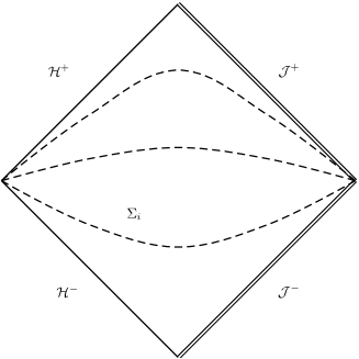
Figure 4: Conformal diagram of ${\cal{M}}_{2}$. Surfaces of constant $t$ are shown dashed, including the initial data surface ${\Sigma_{i}}$. Surfaces at infinity are shown by double lines.

The radial null directions are $\frac{\partial}{\partial u}$ and $\frac{\partial}{\partial v}$, and we choose the following scalings: we will take $\vec{l}$ to be the future pointing ingoing radial null vector field given by

$$\vec{l}=-\frac{2}{H}\frac{\partial}{\partial u},$$ (7)

where

$$H=H(t)=-2\lambda|t_{1}-t|^{\lambda_{2}}|t_{2}-t|^{\lambda_{1}}$$ (8)

and we take $\vec{n}$ to be the future pointing outgoing radial null vector field given by

$$\vec{n}=\frac{\partial}{\partial v}.$$ (9)

With these choices of scaling, $\vec{l}$ is an affinely parametrized null geodesic tangent vector field, and the Newman-Penrose normalization $g_{ab}l^{a}n^{b}=-1$ holds. We note also that in these coordinates, the line element is

$$ds^{2}=Hdudv+r^{2}(u,v)d\Omega^{2}.$$

3 Odd-Parity Perturbations

3.1 The Gerlach-Sengupta formalism

To study perturbations of this spherically symmetric spacetime, we will use the gauge invariant formalism introduced by Gerlach and Sengupta [9]. (We follow the presentation of Martin-Garcia and Gundlach [11].) This is based on the natural 2+2 splitting of a spherically symmetric spacetime, and a multipole decomposition that enables an efficient treatment of the angular dependence of the perturbation.

The metric of a spherically symmetric space-time $({\cal{M}}^{4},g)$ can be written as

$$ds^{2}=g_{AB}(x^{C})dx^{A}dx^{B}+r^{2}(x^{C})\gamma_{\alpha\beta}dx^{\alpha}dx^{\beta},$$ (10)

where $g_{AB}$ is a Lorentzian metric on a 2-dimensional manifold with boundary $M^{2}$ and $\gamma_{\alpha\beta}$ is the standard metric on the unit 2-sphere $S^{2}$. Capital Latin indices represent tensor indices on $M^{2}$, and Greek indices are tensor indices on $S^{2}$. $r(x^{C})$ is a scalar field on $M^{2}$. 4-dimensional space-time indices will be given in lower case Latin. The covariant derivatives on $M^{4}$, $M^{2}$ and $S^{2}$ will be denoted by a semi-colon, a vertical and a colon respectively. $\epsilon_{AB}$ and $\epsilon_{\alpha\beta}$ are covariantly constant anti-symmetric unit tensors with respect to $g_{AB}$ and $\gamma_{\alpha\beta}$. We define

$$v_{A} = \frac{r_{|A}}{r},$$ (11)

$$V_{0} = -\frac{1}{r^{2}}+2{v^{A}}_{|A}+3v^{A}v_{A}.$$ (12)

Writing the energy-momentum tensor as

$$t_{ab}dx^{a}dx^{b}=t_{AB}(x^{C})dx^{A}dx^{B}+Q(x^{C})r^{2}\gamma_{\alpha\beta}dx^{\alpha}dx^{\beta},$$ (13)

the Einstein equations of the spherically symmetric background read

$$G_{AB} = -2(v_{A|B}+v_{A}v_{B})+V_{0}g_{AB}=8\pi t_{AB}$$ (14)

$$\frac{1}{2}G^{\alpha}_{\alpha} = -{\cal{R}}+{v^{A}}_{|A}+v^{A}v_{A}=:8\pi Q,$$ (15)

where $G^{\alpha}_{\alpha}=\gamma^{\alpha\beta}G_{\alpha\beta}$ and ${\cal{R}}$ is the Gaussian curvature of $M^{2}$.

Spherical symmetry of the background allows us to expand the perturbed metric tensor in terms of spherical harmonics. Writing $Y=Y^{m}_{l}$ and suppressing the indices $l,m$ throughout, we have the following bases for scalar, vector and tensor harmonics respectively: $\{Y\}$, $\{Y_{\alpha}:=Y_{:\alpha},S_{\alpha}:=\epsilon_{\alpha}^{\beta}Y_{\beta}\}$ and $\{Y\gamma_{\alpha\beta},Z_{\alpha\beta}:=Y_{\alpha:\beta}+\frac{l(l+1)}{2}Y\gamma_{\alpha\beta},S_{\alpha:\beta}+S_{\beta:\alpha}\}$. These are further classified depending on the transformation properties under spatial inversion ${\vec{x}}\to-\vec{x}$ on the unit sphere: a spherical harmonic with index $l$ is called even if it transforms as $(-1)^{l}$ and is called odd if it transforms as $(-1)^{l+1}$. In the bases above, $Y,Y_{\alpha}$ and $Z_{\alpha\beta}$ are even and $S_{\alpha},S_{(\alpha:\beta)}$ are odd. We note that in the analysis below, the multipole index $l$ only appears in the combination $(l-1)(l+2)$ and so we define ${\ell}=(l-1)(l+2)$.

The perturbation $\delta g_{ab}$ of the metric tensor can then be decomposed as

$$\delta g_{AB} = h_{AB}Y,$$ (16)

$$\delta g_{A\beta} = h^{E}_{A}Y_{:\beta}+h_{A}^{O}S_{\beta},$$ (17)

$$\delta g_{\alpha\beta} = r^{2}K\gamma_{\alpha\beta}Y+r^{2}GZ_{\alpha\beta}+2hS_{(\alpha:\beta)}.$$ (18)

The superscripts $E,O$ stand for even and odd respectively. Note that $h_{AB}$, $\{h_{A}^{E},h_{A}^{O}\}$ and $\{K,G,h\}$ are respectively a 2-tensor, vectors and scalars on $M^{2}$. A similar decomposition of the perturbation of the stress-energy tensor is made:

$$\delta t_{AB} = \Delta t_{AB}Y,$$ (19)

$$\delta t_{A\beta} = \Delta t^{E}_{A}Y_{:\beta}+\Delta t_{A}^{O}S_{\beta},$$ (20)

$$\delta t_{\alpha\beta} = r^{2}\Delta t^{3}\gamma_{\alpha\beta}Y+r^{2}\Delta t^{2}Z_{\alpha\beta}+2\Delta tS_{(\alpha:\beta)}.$$ (21)

In this case, $\Delta t_{AB}$, $\{\Delta t_{A}^{E},\Delta t_{A}^{O}\}$ and $\{\Delta t^{3},\Delta t^{2},\Delta t\}$ are respectively a 2-tensor, vectors and scalars on $M^{2}$.

A complete set of gauge invariant variables is produced as follows. An infinitesmal co-ordinate transformation on the background is generated by a vector field $\vec{\xi}$. Again, we can decompose into even and odd harmonics and consider separately the transformations generated by the 1-form fields

$$\mbox{\boldmath$\xi$}^{E} = \xi_{A}(x^{C})Ydx^{A}+\xi^{E}(x^{C})Y_{:\alpha}dx^{\alpha},$$ (22)

$$\mbox{\boldmath$\xi$}^{O} = \xi^{O}S_{\alpha}dx^{\alpha}.$$ (23)

From the transformed versions of the metric perturbations, one can construct combinations which are independent of the coefficients of $\vec{\xi}$. These combinations are then gauge invariant. As we will only be concerned with the odd parity sector, we give only these terms. The entire odd parity metric perturbation is captured by the gauge invariant co-vector field

$$k_{A} = h_{A}^{O}-h_{|A}+2hv_{A},$$ (24)

and the gauge invariant matter perturbation is described by

$$L_{A} = \Delta t_{A}^{O}-Qh_{A}^{O},$$ (25)

$$L = \Delta t-Qh.$$ (26)

The linearized Einstein equations read

$$\frac{1}{r^{2}}\left[r^{4}\left(\frac{k_{A}}{r^{2}}\right)_{|C}-r^{4}\left(\frac{k_{C}}{r^{2}}\right)_{|A}\right]^{|C}-\frac{{\ell}}{r^{2}}k_{A}=-16\pi L_{A},$$ (27)

$${k^{A}}_{|A}=16\pi L.$$ (28)

The latter equation follows from the former and the linearized conservation equation

$$(r^{2}L_{A})^{|A}={\ell}L.$$ (29)

As noted by Gerlach and Sengupta [9], the vector equation (27) is equivalent to the single scalar equation

$$\left[\frac{1}{r^{2}}(r^{4}\Pi)^{|A}\right]_{|A}-{\ell}\Pi=-16\pi\epsilon^{AB}L_{A|B},$$ (30)

where

$$\Pi:=\epsilon^{AB}(r^{-2}k_{A})_{|B}$$ (31)

is a gauge invariant scalar. $k_{A}$ is recovered from $\Pi$ and $L_{A}$ using

$${\ell}k_{A}=16\pi r^{2}L_{A}-\epsilon_{AB}(r^{4}\Pi)^{|B}.$$ (32)

The quantity $\Pi$ is not only a gauge invariant scalar that, along with $L_{A}$, completely determines the metric perturbation, but as shown in [12], has the tetrad and gauge invariant interpretation of being the perturbation of the Coulomb component $\Psi_{2}$ of the background Weyl tensor.

In order to close the system of perturbation equations, an equation of state must be given for the perturbed spacetime. With this addition, the equations (29) and (30) completely determine the perturbation.

An important point to note is that the formalism described above is incomplete for $l=1$. (There is of course no odd parity $l=0$ perturbation.) For $l=1$, $h$ is not defined, being a coefficient of zero, and so should be considered to be zero. Thus the gauge invariants cannot be constructed. However it is convenient to use the same variables (24)-(26) for all values of $l$. For $l=1$, these variables are only partially gauge invariant, and so gauge-fixing is required. We defer treatment of the case $l=1(\ell=0)$ to Section 5, and so assume until then that $l\geq 2$.

3.2 The matter perturbation

We assume that the non-vacuum portion of the perturbed spacetime is filled with null dust. This allows us to write

$$t_{ab}=(\bar{\rho}+\delta\rho)(\bar{k}_{a}+\delta k_{a})(\bar{k}_{b}+\delta k_{b}),$$

where the barred terms refer to background quantities, so that $\bar{k}_{a}=-\nabla_{a}v$. Retaining only first order terms, we define

$$\delta t_{ab}=\delta\rho\bar{k}_{a}\bar{k}_{b}+\bar{\rho}(\bar{k}_{a}\delta k_{b}+\bar{k}_{b}\delta k_{a}).$$

Comparing with (19)-(21) and recalling that we are considering only odd parity perturbations, we can determine the gauge invariant matter perturbation using (25) and (26): we find $L=0$ and

$$L_{A}=\mu(x^{A})\bar{\rho}\bar{k}_{A},$$ (33)

for some (first order) scalar $\mu$. The evolution of $\mu$ is controlled by (29). In the self-similar coordinates $(t,x)$ we find

$$t\mu_{,t}-\mu_{,x}=0,$$ (34)

which yields

$$\mu=\mu_{0}(te^{x})=\mu_{0}(v)$$

for some arbitrary differentiable function $\mu_{0}$. Thus the matter perturbation is completely determined by the specification of the function $\mu_{0}$ on an initial slice of the form $t=t_{i}\in(0,t_{1})$.

3.3 The master equation

Having completely specified the matter perturbation in terms of an initial data function, we now turn to the only remaining perturbation equation (30). We will refer to this as the master equation and will work in the coordinates $(t,x)$ of Section 2. It is worth repeating that we deal only with the region $0<t<t_{1}$ on which $t$ is a time coordinate. The analysis below follows closely that of [8], and where possible, we will quote results from this paper rather than repeating very similar proofs. We reiterate that $l\geq 2$.

For fixed $\kappa\in\mathbb{R}$, we define $\phi(t,x)=e^{\kappa x}\Pi=r^{\kappa}\Pi$. Then, using (30) and the line element (5), we find that $\phi$ satisfies the inhomogeneous wave equation

$$\alpha\phi_{,tt}+2\beta\phi_{,tx}+\gamma\phi_{,xx}+(\alpha^{\prime}+(6-2\kappa)\beta)\phi_{,t}+(\beta^{\prime}+(6-2\kappa)\gamma)\phi_{,x}$$

$$+((4-\kappa)\beta^{\prime}+(8-6\kappa+\kappa^{2})\gamma-{\ell}e^{\psi})\phi=8\lambda e^{(\kappa-3)x}\mu_{0}(te^{x}),$$ (35)

where $\psi=0$ and

$$\alpha = -2t(1-tG),$$ (36)

$$\beta = 1-2tG,$$ (37)

$$\gamma = 2G,$$ (38)

$$G = \frac{1}{2}-\lambda t.$$ (39)

Modulo the specification of the functional form of $G$, the left hand side of (35), along with (36)-(38), gives the general form of the left hand side of the master equation for the line element (3).

We fix an initial data surface for (35) given by ${\Sigma_{i}}=\{(t,x):t=t_{i},x\in\mathbb{R}\}$ with $t_{i}\in(0,t_{1})$. Our principal concern is how $\phi$ and various of its derivatives representing gauge invariant curvature scalars behave in the approach to the Cauchy horizon, subject to initial regularity conditions imposed at ${\Sigma_{i}}$. Noting that we may write

$$\alpha(t)=-2\lambda t(t_{1}-t)(t_{2}-t)$$

and so $\alpha(t_{1})=0$, we see that this question is rendered nontrivial by virtue of the fact that the Cauchy horizon is a singular hypersurface for the equation (35): the spacelike surfaces $t=$constant become characteristic (null) in the limit $t\to t_{1}$. Prior to the Cauchy horizon, the evolution of $\phi$ proceeds smoothly:

Theorem 1

Let $f,g,\mu_{0}\in C^{\infty}_{0}(\mathbb{R})$ and let $\kappa\in\mathbb{R}$. Then there exists a unique solution $\phi\in C^{\infty}([t_{i},t_{1})\times\mathbb{R},\mathbb{R})$ of the initial value problem consisting of the equation (35) and the initial data

$$\phi|_{\Sigma_{i}}=f,\quad\phi_{,t}|_{\Sigma_{i}}=g.$$

Furthermore, the solution satisfies $\phi|_{t=t_{0}}\in C^{\infty}_{0}(\mathbb{R})$ for all $t_{0}\in[t_{i},t_{1})$.  

The proof of this result is standard and is most easily obtained by rewriting the equation (35) as a first order symmetric hyperbolic system for

$$\vec{\varphi}=\left(\begin{array}[]{c}\phi\\ \alpha\phi_{,t}+\beta\phi_{,x}\\ \phi_{,x}\end{array}\right).$$ (40)

See for example Chapter 12 of [13]. It is convenient to rescale the time coordinate by defining

$$\tau=-\int_{t_{i}}^{t}\frac{ds}{\alpha(s)}.$$ (41)

Then $\tau$ is an analytic function of $t$ on $[t_{i},t_{1})$, $\tau(t_{i})=0$ and $\lim_{t\to t_{1}}\tau=+\infty$. The master equation (35) can be written in first order symmetric hyperbolic form

$$\vec{\varphi}_{,\tau}+A\vec{\varphi}_{,x}+B\vec{\varphi}=\vec{\jmath}$$

where $A,B$ are smooth, bounded matrix functions of $\tau$ on $[0,\infty)$ and $A$ is symmetric with real distinct eigenvalues. The source term $\vec{\jmath}$ is given by

$$\vec{\jmath}=\left(\begin{array}[]{c}0\\ -8\lambda\alpha(t)e^{(\kappa-3)x}\mu_{0}(te^{x})\\ 0\end{array}\right).$$

We wish to analyse the behaviour of the solutions described by Theorem 1, and so we assume until indicated otherwise that the hypotheses of this theorem hold. Then $\vec{\jmath}\in C^{\infty}_{0}([t_{i},t_{1})\times\mathbb{R},\mathbb{R}^{3})$.

We define

$$E_{1}(\tau)=E_{1}[\phi](\tau)=\int_{\mathbb{R}}\|\vec{\varphi}\|^{2}\,dx.$$

The growth of this energy norm is described by the following corollary, again a standard result. We use the notation $\|\vec{a}\|^{2}=(\vec{a},\vec{a})$ (Euclidean inner product) and $\|\vec{a}\|_{2}^{2}=\int_{\mathbb{R}}\|\vec{a}\|^{2}\,dx$ ($L^{2}$ norm). The terms $C_{0},C_{1},...$ represent possibly different constants that depend only on the metric function $G$ and the angular mode number $l$.

Corollary 1

$E_{1}[\phi](\tau)$ is differentiable on $[0,\infty)$ and satisfies

$$E_{1}[\phi](\tau)\leq e^{B_{0}\tau}(E_{1}[\phi](0)+\int_{0}^{\tau}\|\vec{\jmath}(\sigma)\|_{2}^{2}\,d\sigma),$$ (42)

where $B_{0}=\sup_{\tau>0}|I-2B|<+\infty$. Consequently,

$$\int_{\mathbb{R}}|\phi(t,x)|^{2}\,dx \leq e^{B_{0}\tau}(E_{1}[\phi](0)+\int_{0}^{\tau}\|\vec{\jmath}(\sigma)\|_{2}^{2}\,d\sigma),$$

$$\int_{\mathbb{R}}|\phi_{,x}(t,x)|^{2}\,dx \leq e^{B_{0}\tau}(E_{1}[\phi](0)+\int_{0}^{\tau}\|\vec{\jmath}(\sigma)\|_{2}^{2}\,d\sigma),$$

$$\int_{\mathbb{R}}|\phi_{,t}(t,x)|^{2}\,dx \leq C_{1}e^{C_{0}\tau}(E_{1}[\phi](0)+\int_{0}^{\tau}\|\vec{\jmath}(\sigma)\|_{2}^{2}\,d\sigma).$$

 

The bounds on the $L^{2}$ norm of $\phi$ and its derivatives come straight from the definition of $E_{1}(\tau)$: the third requires the use of Minkowski’s inequality and incorporates the exponential growth of $\alpha^{-1}$ as $\tau\to\infty$. As in [8], the growth of these norms in the approach to the Cauchy horizon $\tau\to\infty$ is analysed using a second energy integral.

Let

$$D(t)={\ell}+(\kappa-4)\beta^{\prime}(t)-(\kappa^{2}-6\kappa+8)\gamma(t),$$

and for an arbitrary positive, real-valued differentiable function $K(t)$ define

$$E_{2}[\phi,\mu_{0}](t)=\int_{\mathbb{R}}-\alpha\phi_{,t}^{2}+\gamma\phi_{,x}^{2}+D\phi^{2}+Ke^{2(\kappa-3)x}\mu_{0}^{2}\,dx.$$ (43)

Lemma 1

Let $\kappa\in[0,4]$. Then for all $t\in[t_{i},t_{1}]$, $D(t)\geq 0$ and $D^{\prime}(t)\leq 0$.

Proof: From the definitions (37) and (38) we obtain

$$D(t)={\ell}-(\kappa^{2}-5\kappa+4)+2\lambda t(\kappa^{2}-4\kappa).$$

Thus $D^{\prime}(t)=2\lambda\kappa(\kappa-4)\leq 0$. Then for $t<t_{1}$,

$$D(t) \geq D(t_{1})={\ell}-4+(5-8\lambda t_{1})\kappa-(1-2\lambda t_{1})\kappa^{2}$$

$$\geq (5-8\lambda t_{1})\kappa-(1-2\lambda t_{1})\kappa^{2},$$

where the second inequality uses $l\geq 2$. This last expression, considered as a quadratic function of $\kappa$, is non-negative for $\kappa\in[0,\kappa_{*}]$ where

$$\kappa_{*}=\frac{5-8\lambda t_{1}}{1-2\lambda t_{1}}=4+\frac{2}{1+\nu}>4.$$

This yields $D(t)\geq 0$ on the range indicated.  

Lemma 2

Let $\kappa\in[0,\kappa_{1})$ where

$$\kappa_{1}=\frac{1}{2}(5-4\lambda+\lambda t_{1}^{2})=\frac{1+32\lambda-32\lambda^{2}-\nu}{16\lambda}.$$

Then there exists $t_{c}=t_{c}(\kappa)\in[t_{i},t_{1})$, a constant $C_{0}$ and a choice of $K$ such that $E_{2}[\phi,\mu_{0}](t)\geq 0$ and $\frac{dE_{2}}{dt}\leq C_{0}E_{2}$ for all $t\in[t_{c},t_{1})$.

Proof: Noting that $\kappa_{1}<4$, we see that Lemma 1 applies and so non-negativity of $E_{2}$ is immediate. Write $\tilde{\mu}=e^{(\kappa-3)x}\mu_{0}$. $E_{2}(t)$ is a smooth function of $t$, and smoothness of the solution $\phi$ and of $\mu_{0}$ allow differentiation under the integral sign. The resulting integral is simplified in three steps: (i) integration by parts of the term $\phi_{,x}\phi_{,xt}$ and the removal of a boundary term - permitted as $\phi$ has compact support on each slice $t=$ constant; (ii) removal of the term with $\phi_{,tt}$ by application of the equation (35); (iii) removal of a total derivative containing $\phi_{,t}\phi_{,xt}$. This results in

$$\frac{dE_{2}}{dt} = \int_{\mathbb{R}}\left[(\alpha^{\prime}+2(6-2\kappa))u_{,t}^{2}+2(\beta^{\prime}+(6-2\kappa)\gamma)u_{,t}u_{,x}+\gamma^{\prime}u_{,x}^{2}+D^{\prime}u^{2}\right.$$

$$\left.-16\lambda\tilde{\mu}u_{,t}+2K\tilde{\mu}\tilde{\mu}_{,t}+K^{\prime}\tilde{\mu}^{2}\right]\,dx.$$

In the next round of simplifications, we apply Lemma 1 $(D^{\prime}\leq 0)$, the Cauchy-Schwarz inequality in the form

$$\int_{\mathbb{R}}2\tilde{\mu}u_{,t}\,dx\leq\int_{\mathbb{R}}\tilde{\mu}^{2}+u_{,t}^{2}\,dx$$

and the equation satisfied by $\tilde{\mu}$ (obtained from (34))

$$t\tilde{\mu}_{,t}-\tilde{\mu}_{,x}+(\kappa-3)\tilde{\mu}=0.$$

These yield

$$\frac{dE_{2}}{dt} \leq \int_{\mathbb{R}}\left[(\alpha^{\prime}+2(6-2\kappa)+8\lambda)u_{,t}^{2}+2(\beta^{\prime}+(6-2\kappa)\gamma)u_{,t}u_{,x}+\gamma^{\prime}u_{,x}^{2}\right.$$

$$\left.+(K^{\prime}-2(\kappa-3)\frac{K}{t}+8\lambda)\tilde{\mu}^{2}\right]dx$$

$$=: \int_{\mathbb{R}}I\,dx.$$

For any constant $C>0$, define $I_{R}$ by $I=CI_{E_{2}}+I_{R}$, where $I_{E_{2}}$ is defined so that $E_{2}=\int_{\mathbb{R}}I_{E_{2}}\,dx$. That is,

$$I_{R} = (\alpha^{\prime}+2(6-2\kappa)+8\lambda)u_{,t}^{2}+2(\beta^{\prime}+(6-2\kappa)\gamma)u_{,t}u_{,x}+\gamma^{\prime}u_{,x}^{2}-CDu^{2}$$

$$+(K^{\prime}-(C+\frac{2}{t}(\kappa-3))K+8\lambda)\tilde{\mu}^{2}.$$

The Lemma is proven by showing that there is a choice $C_{0}>0$ of $C$ and a value $t_{c}\in[t_{i},t_{1})$ for which $I_{R}\leq 0$ on $[t_{c},t_{1})$.

For any choice of $C$, there is a positive differentiable function $K$ defined on $[t_{i},t_{1})$ for which the coefficient of $\tilde{\mu}^{2}$ in $I_{R}$ is negative for all $\kappa$ in the range specified. Making this choice and applying Lemma 1, we obtain

$$I_{R} \leq (\alpha^{\prime}+C\alpha+2(6-2\kappa)+8\lambda)u_{,t}^{2}+2(\beta^{\prime}+(6-2\kappa)\gamma)u_{,t}u_{,x}+(\gamma^{\prime}-C\gamma)u_{,x}^{2}$$

$$=: a(t)u_{,t}^{2}+b(t)u_{,t}u_{,x}+c(t)u_{,x}^{2}.$$

Consider next the quadratic form

$$Q(X,Y;t)=a(t)X^{2}+b(t)XY+c(t)Y^{2}.$$

We find

$$a(t_{1}) = 2(4\kappa-5+4\lambda+\lambda t_{1}^{2}),$$

$$b(t_{1}) = -\frac{4}{t_{1}}(2\kappa-5-\lambda t_{1}^{2}),$$

$$c(t_{1}) = -2(\lambda+\frac{C}{t_{1}}).$$

We note that $c(t_{1})<0$ for any $C>0$ and $\lambda\in(0,1/16)$. The term $a(t_{1})$ is negative due to the assumed bound on $\kappa$. Then the discriminant is also negative if $C$ is chosen sufficiently large. So $Q(X,Y;t_{1})$ is negative definite. Then by continuity of the coefficients $a,b,c$, the quadratic form $Q(X,Y;t)=a(t)X^{2}+b(t)XY+c(t)Y^{2}$ is negative definite for all $t$ sufficiently close to $t_{1}$. That is, there exists some $t_{c}<t_{1}$ such that $Q(X,Y;t)\leq 0$ for all $X,Y\in\mathbb{R}$ and $t\in[t_{c},t_{1})$ with equality holding iff $X=Y=0$. We note however that the value of $t_{c}$ will depend on $\kappa$, with $t_{c}\to t_{1}$ as $\kappa\to\kappa_{1}$. This however does not affect the proof, which is now completed.  

Remark 2.1

By minimising $\kappa_{1}(\lambda)$ for $\lambda\in(0,1/16)$, we could restate Lemma 2 with the simpler requirement $\kappa\in[0,\frac{5}{2})$.

We can now give our first main result.

Theorem 2

Let $\phi$ be a solution of (35) that is subject to the hypotheses of Theorem 1 and Lemma 2. Then the energy $E_{2}[\phi,\mu_{0}](t)$ of the solution satisfies the a priori bound

$$E_{2}[\phi,\mu_{0}](t)\leq C_{1}E_{1}[\phi](0)+C_{2}J_{\kappa}[\mu_{0}],\quad t\in[t_{i},t_{1})$$

where

$$J_{\kappa}[\mu_{0}]=\int_{\mathbb{R}}e^{2(\kappa-3)x}\mu_{0}^{2}(t_{i}e^{x})\,dx.$$

Proof: We point out first how to convert the bounds of Corollary 1 to a priori bounds. To do this, we exploit the self-similar nature of the solution $\mu$ of the matter perturbation equation (34). We have

$$\|\vec{\jmath}\|^{2}_{2}(\tau)=64\alpha^{2}(t)\int_{\mathbb{R}}e^{2(\kappa-3)x}\mu_{0}^{2}(te^{x})\,dx.$$

A change of variable in the integral yields

$$\|\vec{\jmath}\|^{2}_{2}(\tau)=\left(\frac{\alpha(t)}{\alpha(t_{i})}\right)^{2}\left(\frac{t_{i}}{t}\right)^{2(\kappa-3)}J_{\kappa}[\mu_{0}].$$

Then making the appropriate change of variables using (41), we obtain

$$\int_{0}^{\tau}\|\vec{\jmath}\|^{2}_{2}(\sigma)\,d\sigma = J_{\kappa}[\mu_{0}]\int_{t_{i}}^{t}\frac{-\alpha(s)}{(\alpha(t_{i}))^{2}}\left(\frac{t_{i}}{s}\right)^{2(\kappa-3)}\,ds$$

$$=: h(t)J_{\kappa}[\mu_{0}]\leq C_{0}J_{\kappa}[\mu_{0}].$$

From Corollary 1, we can write

$$E_{2}[\phi,\mu_{0}](t)\leq d(t)(E_{1}[\phi](0)+C_{2}J_{\kappa}[\mu_{0}]),$$ (44)

where $d(t)$ is a smooth positive function of $t$ that diverges in the limit $t\to t_{1}$. However, $d(t_{c})$ is finite, where $t_{c}$ is the value of $t$ identified in Lemma 2. From time $t_{c}$ onwards, $E_{2}$ obeys the differential inequality of this lemma, which may be integrated to yield

$$E_{2}(t)\leq e^{C_{0}(t-t_{c})}E_{2}(t_{c}),\quad t\in[t_{c},t_{1}).$$ (45)

Combining (44) and (45) yields the desired result.  

Theorem 3

Let $\phi$ be a solution of (35) that is subject to the hypotheses of Theorem 1 and Lemma 2. Then $\phi$ is uniformly bounded on $[t_{i},t_{1})\times\mathbb{R}$: there exist positive constants $C_{1}$ and $C_{2}$ such that

$$|\phi(t,x)|\leq C_{1}E_{1}[\phi](0)+C_{2}J_{\kappa}[\mu_{0}],\quad t\in[t_{i},t_{1}),x\in\mathbb{R}.$$ (46)

Proof: Theorem 2 provides an a priori bound for the $H^{1,2}$ norm of $\phi$: for all $t\in[t_{i},t_{1})$,

$$\int_{\mathbb{R}}\phi^{2}+\phi_{,x}^{2}dx\leq C_{1}E_{1}[\phi](0)+C_{2}J_{\kappa}[\mu_{0}].$$

The pointwise bound arises immediately on application of the Sobolev inequality for $v\in C^{\infty}_{0}(\mathbb{R})$:

$$|v(x)|^{2}\leq\frac{1}{2}\left\{\int_{\mathbb{R}}|v(y)|^{2}+|v^{\prime}(y)|^{2}\,dy\right\}.$$

See p. 1057 of [14] for a proof of this inequality.  

Remark 3.1

Note that by differentiating (35) with respect to $x$, we can obtain results similar to Theorems 1-3 for any spatial derivative of $\phi$. The bounding term in the inequalities corresponding to (46) will involve sums of terms of the form $E_{1}[\frac{\partial^{n}\phi}{\partial x^{n}}](0)$ and $J_{\kappa}[\mu_{0}^{(n)}]$.

Remark 3.2

Of principal concern in this paper is the behaviour of the field $\Pi$ and those of its derivatives representing the perturbed Weyl curvature scalars. Theorem 3 shows that $\Pi$ is bounded in the limit as the Cauchy horizon is approached ($t\to t_{1}$). However this does not imply that $\lim_{t\to t_{1}}\Pi(t,x)$ exists for any $x\in\mathbb{R}$. We will show now that this is in fact the case; indeed we can show that $\Pi|_{t=t_{1}}\in C^{\infty}(\mathbb{R})$. In [8], the corresponding limit function was erroneously assumed to exist on the basis of the equivalent to Theorem 3. This assumption can be shown to be true by applying the argument below to that paper, and so does not affect the results of that paper.

In order to get from the bound of Theorem 3 to the existence of the limit $\lim_{t\to t_{1}}\phi(t,x)$, we need some control over the time derivative of $\phi$ as the Cauchy horizon is approached. This is provided by the following lemma, which relies on treating (35) as a first order transport equation for $\phi_{,t}$.

Lemma 3

Let $\phi$ be a solution of (35) that is subject to the hypotheses of Theorem 1 and Lemma 2. Then $\phi_{,t}$ is uniformly bounded on $[t_{i},t_{1})\times\mathbb{R}$: there exist positive constants $C_{0},C_{1},...$ such that

$$|\phi_{,t}(t,x)| \leq C_{0}E_{1}[\phi](0)+C_{1}E_{1}[\phi_{,x}](0)+C_{2}E_{1}[\phi_{,xx}](0)$$

$$+C_{3}J_{\kappa}[\mu_{0}]+C_{4}J_{\kappa}[\mu_{0}^{\prime}]+C_{5}J_{\kappa}[\mu_{0}^{\prime\prime}],\quad t\in[t_{i},t_{1}),x\in\mathbb{R}.$$

Proof: Define $\chi=\phi_{,t}$. Then (35) can be written

$$\alpha\chi_{,t}+2\beta\chi_{,x}+(\alpha^{\prime}+(6-2\kappa)\beta)\chi=f(t,x),$$ (47)

where the right hand side depends linearly on $\mu_{0}$ and the zeroth, first and second spatial derivatives of $\phi$. Then $f$ is smooth and has compact support on each slice $t=$constant. If we write (35) as

$$L[\phi]=a_{0}(t,x)\mu_{0}(te^{x}),$$

then differentiation with respect to $x$ shows that $\phi_{,x}$ and $\phi_{,xx}$ satisfy equations with identical first and second order derivative coefficients:

$$L[\phi_{,x}] = b_{0}(t,x)\mu_{0}(te^{x})+b_{1}(t,x)\mu_{0}^{\prime}(te^{x}),$$

$$L[\phi_{,xx}] = c_{0}(t,x)\mu_{0}(te^{x})+c_{1}(t,x)\mu_{0}^{\prime}(te^{x})+c_{2}(t,x)\mu_{0}^{\prime\prime}(te^{x}).$$

We can therefore apply Theorem 3 to $\phi_{,x}$ and $\phi_{,xx}$: the only difference in the result will be that the bounding terms will depend also on the $L^{2}$ norms of the first and second derivatives of $\phi$ and $\mu_{0}$ at $t=t_{i}$. Then by linearity, we can bound $f$ by a similar a priori term. The bound for $u$ then arises by straightforward integration of the first order transport equation (47). See Theorem 6 of [8].  

Theorem 4

Let $\phi$ be a solution of (35) that is subject to the hypotheses of Theorem 1 and Lemma 2. Then $\phi_{{\cal{H}}^{+}}:=\lim_{t\to t_{1}}\phi(t,\cdot)\in C^{\infty}(\mathbb{R})$ and satisfies the bound

$$|\phi_{{\cal{H}}^{+}}(x)|\leq C_{1}E_{1}[\phi](0)+C_{2}J_{\kappa}[\mu_{0}],\quad x\in\mathbb{R}.$$

Proof: Fix $x\in\mathbb{R}$ and consider a sequence $\{t^{(n)}\}_{n=1}^{\infty}\subset[t_{i},t_{1})$ that converges to $t_{1}$. For all $m,n\geq 1$, we can apply the mean value theorem to get

$$|\phi(t^{(m)},x)-\phi(t^{(n)},x)|=|\phi_{,t}(t_{*},x)||t^{(m)}-t^{(n)}|$$ (48)

for some $t_{*}$ between $t^{(m)}$ and $t^{(n)}$. Using the bound of Lemma 3, we see that $\phi(t^{(m)},x)$ is a Cauchy sequence of real numbers, and so for each $x\in\mathbb{R}$, $\lim_{t\to t_{1}}\phi(t,x)$ exists. Hence $\phi_{{\cal{H}}^{+}}$ is defined. We can apply an analogous argument to all the spatial derivatives of $\phi$. It remains to show that

$$\frac{d}{dx}\left\{\phi_{{\cal{H}}^{+}}\right\}=\lim_{t\to t_{1}}\phi_{,x}(t,x).$$

(Again, an analogous argument will apply to higher spatial derivatives.) But this follows by uniform convergence of the sequence of functions $\phi(t^{(n)},x)$ to $\phi_{{\cal{H}}^{+}}$, which in turn follows from (48) and the uniform bound of Lemma 3. To obtain the bound in the statement of the theorem, we take the limit $t\to t_{1}$ of the corresponding bound in Theorem 3. This is permitted as the bounding term is independent of $t$.  

We conclude this section by extending the results of Theorems 1-4 to the case where the initial data lie in appropriate Sobolev spaces. This is important as it will allow the perturbation to be non-zero at the axis $r=0$. The results so far relate to the case where the initial data and the corresponding solutions are supported away from $r=0$. This is an undesirable feature, as we would ideally like to consider a perturbation that arises from data imposed on a globally regular initial data slice of the space-time: our $t=t_{i}$ slice is singular at the origin. Such a regular slice would intersect the past null cone, and we should certainly consider the case where the support of the initial data also does so. We can deal with such data by taking the limit of a sequence of test function ($C^{\infty}_{0}$) data in an appropriate Sobolev space.

Theorem 5

Let $\kappa\in[0,\kappa_{1})$ and let $\phi=e^{\kappa x}\Pi$ and define $\tilde{\mu}(x)=e^{(\kappa-3)x}\mu_{0}(x)=e^{(\kappa-3)x}\mu(t_{i}e^{x})$.

• Let $f\in H^{1,2}(\mathbb{R})$, $g\in L^{2}(\mathbb{R})$, $\tilde{\mu}\in L^{2}(\mathbb{R})$. Then there exists a unique solution $\phi\in C([t_{i},t_{1}),H^{1,2}(\mathbb{R}))$ of the initial value problem consisting of (35) with initial data $\phi|_{{\Sigma_{i}}}=f$, $\phi_{,t}|_{\Sigma_{i}}=g$. The solution satisfies the a priori bound

  $$|\phi(t,x)|\leq C_{0}E_{1}[\phi](0)+C_{2}J_{\kappa}[\tilde{\mu}],\quad t\in[t_{i},t_{1}),x\in\mathbb{R}.$$

• Let $f\in H^{3,2}(\mathbb{R})$, $g\in H^{2,2}(\mathbb{R})$, $\tilde{\mu}\in H^{2,2}(\mathbb{R})$. Then there exists a unique solution $\phi\in C([t_{i},t_{1}],H^{1,2}(\mathbb{R}))$ of the initial value problem consisting of (35) with initial data $\phi|_{{\Sigma_{i}}}=f$, $\phi_{,t}|_{\Sigma_{i}}=g$. The solution satisfies the a priori bound

  $$|\phi(t,x)|\leq C_{0}E_{1}[\phi](0)+C_{2}J_{\kappa}[\tilde{\mu}],\quad t\in[t_{i},t_{1}],x\in\mathbb{R},$$

  and its time derivative satisfies

  $$|\phi_{,t}(t,x)| \leq C_{0}E_{1}[\phi](0)+C_{1}E_{1}[\phi_{,x}](0)+C_{2}E_{1}[\phi_{,xx}](0)$$

  $$+C_{3}J_{\kappa}[\tilde{\mu}]+C_{4}J_{\kappa}[\tilde{\mu}^{\prime}]+C_{5}J_{\kappa}[\tilde{\mu}^{\prime\prime}],\quad t\in[t_{i},t_{1}],x\in\mathbb{R}.$$

Proof: We give just the outline of the proof, which is nearly identical to Theorems 5 and 7 of [8] and which relies on a standard PDE technique. For part (i), we consider sequences of test functions $\{f_{(n)}\}_{n=0}^{\infty}$, $\{g_{(n)}\}_{n=0}^{\infty}$, $\{{\tilde{\mu}}_{(n)}\}_{n=0}^{\infty}$ and apply Theorems 1-3 to obtain a sequence of smooth solutions $\{\phi_{(n)}\}_{n=0}^{\infty}\subset C^{\infty}([t_{i},t_{1})\times\mathbb{R})$ satisfying the bounds of Theorems 2 and 3 above. By exploiting linearity of the equation and the fact that $C^{\infty}_{0}(\mathbb{R})$ is dense in the Banach spaces $L^{2}$ and $H^{k,2}$ for $k=1,2,3\dots$, we can legitimately take the limit of relevant inequalities to prove the stated results. The proof of part (ii) is similar, but higher order Sobolev spaces must be invoked due to the form of the inequality of Lemma 2.  

4 Gauge Invariant Curvature Scalars

As seen above, the odd parity perturbation of Vaidya spacetime is completely described by the vector $L_{A}$ and the scalar $\Pi$. The latter quantity plays a dual role: on the one hand it is a potential for the gauge invariant metric perturbation $k_{A}$ (see (32)) and on the other, is the gauge invariant perturbation of the Coulomb component $\Psi_{2}$ of the Weyl tensor [12]. For at least two reasons, it is desirable to have a full set of gauge invariant scalars that describes the perturbation of the Weyl tensor.

First, one prefers scalars as these avoid the problems presented by an inappropriate choice of coordinates. The components of a non-zero rank tensor may blow-up, with the blow-up inadvertently ascribed to singular behaviour rather than the wrong choice of coordinates.

Second, the metric and matter perturbations alone do not capture the whole physical picture (neither of course does the Weyl tensor alone). Perhaps the best example of this is the case of perturbations impinging on the inner (Cauchy) horizon of a charged or spinning black hole. Here the metric perturbation remains continuous (but not differentiable) and the Weyl curvature blows up, a scenario described as mass inflation [10]. This has been described rigourously in [15].

As shown in [12], the perturbed Weyl scalars can be defined in a gauge invariant manner in the case of odd parity perturbations. Using a null tetrad $\{\vec{l},\vec{n},\vec{m},\vec{m}^{*}\}$ where the asterisk represents complex conjugation and following the notation of [16] for the Weyl scalars $\Psi_{0},\dots,\Psi_{4}$, the perturbed Weyl scalars are given by

$$\delta\Psi_{0} = \left.\frac{Q_{0}}{2r^{2}}\right.l^{A}l^{B}k_{A|B},$$ (49)

$$\delta\Psi_{1} = \left.\frac{Q_{1}}{r}\right.\left[(r^{2}\Pi)_{|A}l^{A}-\frac{4}{r^{2}}k_{A}l^{A}\right],$$ (50)

$$\delta\Psi_{2} = {Q_{2}}\Pi,$$ (51)

$$\delta\Psi_{3} = \left.\frac{Q^{*}_{1}}{r}\right.\left[(r^{2}\Pi)_{|A}n^{A}-\frac{4}{r^{2}}k_{A}n^{A}\right],$$ (52)

$$\delta\Psi_{4} = \left.\frac{Q^{*}_{0}}{2r^{2}}\right.n^{A}n^{B}k_{A|B},$$ (53)

where the functions $Q_{i},i=0,1,2$ depend only on the angular coordinates. In this definition, we restrict to the preferred sets of null tetrads defined on the spherically symmetric background for which $\vec{l}$ and $\vec{n}$ are the principal null directions of the background. Then there remains a scaling freedom in these definitions. Under the spin-boost transformation

$$(\vec{l},\vec{n})\to(A\vec{l},A^{-1}\vec{n})$$

we find

$$\delta\Psi_{i}\to A^{2-i}\delta\Psi_{i}$$

for $i=0,\dots 4$. Thus we cannot ascribe direct physical significance to the values of $\delta\Psi_{i}$ (except for $i=2$). However the terms

$$\delta P_{-1} = |\delta\Psi_{0}\delta\Psi_{4}|^{1/2},$$ (54)

$$\delta P_{0} = \delta\Psi_{2},$$ (55)

$$\delta P_{1} = |\delta\Psi_{1}\delta\Psi_{3}|^{1/2}$$ (56)

are fully invariant perturbation scalars: i.e. they are first order scalars which are both gauge and tetrad invariant.

4.1 The master equation in null coordinates

It is straightforward to calculate $\delta\Psi_{0},\dots\delta\Psi_{4}$ in the coordinates $(t,x)$ of Section 3. However it is less straightforward to determine whether or not the resulting quantities are finite at the Cauchy horizon $t=t_{1}$: we encounter terms involving products of negative powers of the term $H(t)$ of Section 2 with first and second time $(t)$ derivatives of $\Pi$. While we know that the first time derivative of $\Pi$ is bounded, we have no information regarding the behaviour of the second time derivative at the Cauchy horizon. It turns out that we can circumvent this problem by calculating the scalars (49)-(53) in the null coordinates $(u,v)$ of Section 2. This approach also necessitates rewriting the equation (35) in these null coordinates. The result of this is as follows. Let

$$\Psi=r^{3}\Pi=e^{3x}\Pi.$$

Then we find

$$\Psi_{,uv}+\tilde{V}(u,v)\Psi=\tilde{F},$$ (57)

where

$$\tilde{V} = -\frac{1}{4uv}(\alpha\beta^{\prime}+1-\beta^{2}-{\ell}\alpha),$$

$$\tilde{F} = -2\lambda\frac{\alpha}{uv}\mu_{0}(v).$$

In these coordinates, we find that

$$\delta\Psi_{0}=-\frac{4}{H^{2}}(\Psi_{,uu}+\frac{2-\alpha^{\prime}}{2u}\Psi_{,u})Q_{1}$$ (58)

for which the problem mentioned above remains. However the following relabelling of the null cones resolves the problem.

Define

$$X=|u|^{\frac{1}{\lambda_{1}}}=|t_{1}-t||t_{2}-t|^{\frac{\nu-1}{\nu+1}}\exp(\frac{x}{\lambda_{1}}),\quad Y=v=te^{x}.$$ (59)

We note that $X=0$ at the Cauchy horizon $t=t_{1}$. Then (57) - that is, the master equation - takes the form

$$\Psi_{,XY}+V(X,Y)\Psi=F(X,Y),$$ (60)

where

$$V(X,Y)=-\frac{1}{2}\lambda_{1}\lambda|t_{2}-t|^{\frac{2}{1+\nu}}\exp(-(\frac{1+3\nu}{1+\nu})x)$$

and

$$F(X,Y)=4\lambda_{1}\lambda^{2}|t_{2}-t|^{\frac{2}{1+\nu}}\exp(-(\frac{1+3\nu}{1+\nu})x)\mu_{0}(Y).$$

Note that for any fixed $Y=v>0$, $V$ and $F$ are analytic functions of $X$ at $X=0$. Moreover, there exists $C>0$ and sequences of smooth functions $\{V_{n}\}_{n=0}^{\infty}$, $\{F_{n}\}_{n=0}^{\infty}$ such that

$$V(X,Y)=\sum_{n=0}^{\infty}V_{n}(Y)X^{n},\quad F(X,Y)=\sum_{n=0}^{\infty}F_{n}(Y)X^{n},\quad|X|<C.$$ (61)

Combining the high degree of regularity of the coefficients of (60) with the results of Section 3 yields the following.

Theorem 6

Let $f,g,\mu_{0}\in C^{\infty}_{0}(\mathbb{R})$ and let $\Pi\in C^{\infty}([t_{i},t_{1})\times\mathbb{R})\cap C^{\infty}(\{t=t_{1}\}\times\mathbb{R})$ be the unique solution of the initial value problem consisting of (35) with initial data

$$\Pi|_{\Sigma_{i}}=f,\quad\Pi_{,t}|_{\Sigma_{i}}=g.$$

Let $X,Y$ be as defined in (59). Then there exists $X_{0}>0$ such that $\Psi=e^{3x}\Pi$ satisfies $\Psi\in C^{\infty}(\Omega)$ where

$$\Omega=\{(X,Y):0\leq X\leq X_{0},Y>0\}.$$

Thus all $X\!\!-$ and $Y\!\!-$derivatives of $\Psi$ are finite at the Cauchy horizon $X=0$.

Proof: Consider the characteristic rectangle

$$R=\{(X,Y):0\leq X\leq X_{0},Y_{0}\leq Y\leq Y_{1}\}$$

where $X_{0}>0$ and $0<Y_{0}<Y_{1}$. Applying Theorem 1 and Theorem 4 with $\kappa=0$ and noting that the coordinate transformation $(t,x)\to(u,v)$ is a homeomorphism on $R$ for sufficiently small $X_{0}$, we see that $\Psi\in C^{0}(R,\mathbb{R})$. Then rewriting (60) as

$$\Psi_{,XY}=-V\Psi+F=:Q(X,Y),$$

we have $Q\in C^{0}(R,\mathbb{R})$. For any $Y\in(Y_{0},Y_{1}]$, we can then integrate to obtain

$$\frac{\partial\Psi}{\partial X}(X,Y)-\frac{\partial\Psi}{\partial X}(X,Y_{0})=\int_{Y_{0}}^{Y}Q(X,Z)\,dZ.$$

We can choose $Y_{0}$ to be small enough so that the ingoing null ray $Y=Y_{0}$ lies outside the support of $\Psi$ (see Figure 5). Then $\frac{\partial\Psi}{\partial X}(X,Y_{0})=0$, and

$$\frac{\partial\Psi}{\partial X}(X,Y)=\int_{Y_{0}}^{Y}Q(X,Z)\,dZ,$$

giving $\Psi_{,X}\in C^{0}(R,\mathbb{R})$. A similar argument yields $\Psi_{,Y}\in C^{0}(R,\mathbb{R})$, and so $\Psi\in C^{1}(R,\mathbb{R})$. Continuing this argument inductively, we obtain $\Psi\in C^{\infty}(R,\mathbb{R})$ for all $Y_{0}$ taken sufficiently small and all $Y_{1}>0$.  

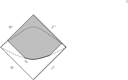
Figure 5: Spread of the support of the field (shaded), with initial data with compact support $S_{0}\subset\Sigma_{i}$. There are ingoing null rays from $\Sigma_{i}$ to ${\cal{H}}^{+}$ which lie outside the support of the field.

Remark 6.1

It is reasonable to ask why we have not simply stated the entire problem in the coordinates $(X,Y)$ and deduced finiteness of $\Psi$ - and hence $\Pi$ - at the Cauchy horizon by writing down a very simple existence and uniqueness theorem for the characteristic initial value problem consisting of (60) with characteristic data $\Psi|_{X=X_{0}},\Psi|_{Y=Y_{0}}\in C^{\infty}(0,+\infty)$. The answer to this is that this formulation of the problem assumes that the field $\Pi$ is a smooth function of the retarded null coordinate $X$ at the Cauchy horizon. But the question of whether or not this is a valid assumption is the very point that we are attempting to address here, with respect to finite initial Cauchy data posed on a hypersurface that precedes the Cauchy horizon.

4.2 The perturbed Weyl scalars

There is a further advantage of the coordinates $(X,Y)$. Not only does the master equation assume the simple form (60), but we find that the perturbed Weyl scalars assume a very simple form when expressed in these coordinates. Using (58) and (59), we find

$$\delta\Psi_{0}=-\frac{4}{\lambda_{1}^{2}H^{2}}X^{\frac{\nu-1}{\nu}}(\Psi_{,XX}+(1-\frac{\lambda_{1}}{2}\alpha^{\prime})X^{-1}\Psi_{,X})e^{-x}Q_{0}.$$ (62)

Using (8), (36), and (59), we have

$$H^{-2}X^{\frac{\nu-1}{\nu}} = \frac{1}{4\lambda^{2}}|t_{2}-t|^{-\frac{4}{1+\nu}}\exp(2(\frac{\nu-1}{\nu+1})x),$$

$$(1-\frac{\lambda_{1}}{2}\alpha^{\prime})X^{-1} = \lambda_{1}\lambda(2t_{2}-t_{1}-3t)(t_{2}-t)^{\frac{\nu-1}{\nu+1}}\exp(-(\frac{2\nu}{1+\nu})x).$$

Thus $\delta\Psi_{0}$ is finite at the Cauchy horizon $X=0(t=t_{1})$. This also holds for the other perturbed Weyl curvature scalars. Finiteness is immediate for $\delta\Psi_{2}$, which is essentially $\Pi$. The other gravitational radiation scalar, representing outgoing radiation, is found to be

$$\delta\Psi_{4}=\{(\Psi_{,YY}+(1-4\lambda t)e^{-x}\Psi_{,Y}-4\lambda e^{-2x}\Psi)e^{x}-4\lambda(\mu_{0}^{\prime}(Y)-2\lambda te^{-x}\mu_{0}(Y))\}e^{-2x}Q_{0}^{*}.$$ (63)

It is immediate from Theorem 6 that this is finite at the Cauchy horizon. For the two remaining scalars, we find

$$\delta\Psi_{1}=\left\{\frac{2}{\lambda_{1}}({\ell}-4)H^{-1}X^{\frac{\nu-1}{2\nu}}e^{x}\Psi_{,X}+({\ell}+4)\Psi\right\}e^{-3x}\frac{Q_{1}}{{\ell}}$$ (64)

with

$$H^{-1}X^{\frac{\nu-1}{2\nu}}=-\frac{1}{2\lambda}|t_{2}-t|^{-\frac{2}{\nu+1}}\exp((\frac{\nu-1}{\nu+1})x),$$

while

$$\delta\Psi_{3}=\left\{({\ell}+4)\Psi_{,Y}-\frac{1}{2}({\ell}-4)t(1-2\lambda t)Y^{-1}\Psi+64\pi\bar{\rho}e^{x}\mu_{0}(Y)\right\}e^{-2x}\frac{Q_{1}^{*}}{{\ell}}.$$ (65)

Thus these scalars are also finite at the Cauchy horizon. Thus we have proven the following.

Theorem 7

Subject to the hypotheses of Theorem 6, the perturbed Weyl scalars (50)-(53), calculated with respect to the null vectors $\{\vec{l},\vec{n}\}$ defined in (7) and (9), are finite at all points of $\{(t,x):t_{i}\leq t\leq t_{1},x\in\mathbb{R}\}$. In particular, the perturbed Weyl scalars are finite at the Cauchy horizon ${{\cal{H}}^{+}}$.  

Remark 7.1

Having found a null tetrad in which all the perturbed Weyl scalars are finite at the Cauchy horizon, it is clear that the fully invariant scalars $\delta P_{i},i=0,\pm 1$ are also finite thereat. A difficulty of interpretation of the $\delta\Psi_{i}$ would only arise if one found (say) vanishing of $\delta\Psi_{0}$ and divergence of $\delta\Psi_{4}$ at the Cauchy horizon. In such a case, recourse to the calculation of $\delta P_{-1}$ would be essential.

As in the previous section, we wish to extend the present results to initial data of the type considered in Theorem 5. As in the proof of that theorem, the principal requirement is the existence of a priori bounds for the relevant quantities.

Theorem 8

Subject to the hypotheses of Theorem 6, the following a priori bounds hold: for each $i\in\{0,\dots,4\}$, there exist constants $C_{0}^{(i)},C_{1}^{(i)},\dots,C_{5}^{(i)}$ that depend only on $\lambda$ and $\kappa$ such that for all $(t,x)\in[t_{i},t_{1}]\times\mathbb{R}$,

$$|e^{\kappa x}\delta\Psi_{i}(t,x)| \leq C_{0}^{(i)}E_{1}[\phi](0)+C_{1}^{(i)}E_{1}[\phi_{,x}](0)+C_{2}^{(i)}E_{1}[\phi_{,xx}](0)$$ (66)

$$+C_{3}^{(i)}J_{\kappa}[\mu_{0}]+C_{4}^{(i)}J_{\kappa}[\mu_{0}^{\prime}]+C_{5}^{(i)}J_{\kappa}[\mu_{0}^{\prime\prime}].$$

Proof: We consider first the case $\kappa=0$. For $i=2$, the bound (66) is immediate from the definition (51) and from Theorems 2 and 3 (where we let $\kappa=0$ in those theorems). A straightforward calculation shows that

$$\delta\Psi_{1}=\left[a(t)\Pi_{,t}+b(t)\Pi_{,x}+c(t)\Pi\right]\frac{Q_{1}}{{\ell}},$$

where here and in the rest of this proof, $a,b,c,\dots$ represent functions of $t$ that are smooth and uniformly bounded on $[t_{i},t_{1}]$, and which may change from line to line. Similarly, we find

$$\delta\Psi_{3}=\left[a(t)\Pi_{,t}+b(t)\Pi_{,x}+c(t)\Pi+128\pi\lambda e^{-3x}\mu_{0}(te^{x})\right]\frac{Q_{1}}{{\ell}}.$$

The result follows by application of Theorems 2 and 3 to $\Pi$ and analogous results for $\Pi_{,x}$ (see Remark 3.1) and by application of Lemma 3 which provides the bound for $\Pi_{,t}$. Again, we take $\kappa=0$ in these results.

To obtain bounds on $\delta\Psi_{0}$ and $\delta\Psi_{4}$, we exploit the form (60) that the master equation takes in the null coordinates $(X,Y)$. Integrating, and using the fact that $\Psi$ is identically zero for sufficiently small values of $Y$, we can write

$$\Psi_{,X}(X,Y)=\int_{0}^{Y}-V(X,Z)\Psi(X,Z)+F(X,Z)\,dZ.$$

Differentiating under the integral sign (which is permitted by smoothness) gives

$$\Psi_{,XX}=\int_{0}^{Y}-V_{,X}\Psi+V\Psi_{,X}+F_{,X}\,dZ.$$

This can be written as

$$\Psi_{,XX}=\int_{0}^{Y}[a(t)\Pi_{,t}+b(t)\Pi_{,x}+c(t)\Pi+d(t)e^{-3x}\mu_{0}(Z)]\exp(2(\frac{1-\nu}{1+\nu})x)\,dZ,$$

where in the integral it is understood that $t=t(X,Z)$ and $x=x(X,Z)$. The term in the integrand in square brackets can be bounded by an a priori term of the form in the statement of the theorem; we use $M$ to represent such a term. Then

$$|\Psi_{,XX}|\leq M\int_{0}^{Y}Z^{2(\frac{1-\nu}{1+\nu})}\,dZ,$$

wher we have used the definition $Y=te^{x}$ and absorbed a function of type $a(t)$ into $M$. Evaluating the integral, we see that

$$|H^{-2}X^{\frac{\nu-1}{\nu}}e^{-x}\Psi_{,XX}|\leq a(t)M=M.$$

In a similar manner, we can show that

$$|(1-\frac{\lambda_{1}}{2}\alpha^{\prime})H^{-2}X^{-\frac{1}{\nu}}e^{-x}\Psi_{,X}|\leq M.$$

Hence by (62), the theorem is proven for $i=0$. The case $i=4$ is similar (but more straightforward).

For values of $\kappa$ with $\kappa\neq 0$, we simply point out that by virtue of the self-similar and linear nature of the equation (35) and the linearity of the $\delta\Psi_{i}$ in $\Pi$ and $\mu$, an identical argument to that above applies.  

We conclude by writing down the result describing bounds on the perturbed Weyl scalars that ensues by considering data of the form dealt with in Theorem 5. We omit the proof, noting that this proceeds in exactly the way described in the summary proof of Theorem 5: we apply Theorem 8 to a sequence of solutions generated by data in $C^{\infty}_{0}$. Then the hypothesis that the limit of the data exists and lies in (some) $H^{n,2}$ and the existence of the a priori bounds in Theorem 8 ensures the existence of the limits of those bounds.

Theorem 9

Let $\kappa\in[0,\kappa_{1})$ and let $\phi=e^{\kappa x}\Pi$ and define $\tilde{\mu}(x)=e^{(\kappa-3)x}\mu_{0}(x)=e^{(\kappa-3)x}\mu(t_{i}e^{x})$. Let $f\in H^{3,2}(\mathbb{R})$, $g\in H^{2,2}(\mathbb{R})$, $\tilde{\mu}\in H^{2,2}(\mathbb{R})$. Then the perturbed Weyl scalars (49)- (53) calculated with respect to the unique solution $\phi\in C([t_{i},t_{1}],H^{1,2}(\mathbb{R}))$ of the initial value problem consisting of (35) with initial data $\phi|_{{\Sigma_{i}}}=f$, $\phi_{,t}|_{\Sigma_{i}}=g$ satisfy the a priori bounds (66) of Theorem 8. In particular, the perturbed Weyl scalars are finite at the Cauchy horizon $ch^{+}$.  

5 The $l=1$ Perturbation.

We return now to the $l=1$ perturbation. The treatment is considerably more straightforward, but at the loss of full gauge invariance of some of the results. The crucial difference for $l=1$ is that the metric perturbation quantity $k_{A}$ is no longer gauge invariant. We find that under the infinitesmal transoformation generated by $\mbox{\boldmath$\xi$}=\xi S_{\alpha}dx^{\alpha}$, $k_{A}$ transforms as

$$k_{A}\to k_{A}-r^{2}(r^{-2}\xi)_{,A}.$$

Furthermore, the equation (28) no longer holds. However the quantity $\Pi$ is gauge invariant, and the equation (32) holds. Since $\ell=0$, this equation is readily solved once $L_{A}$ is determined. This is done following the same procedure as for $l\geq 2$: we find $L_{A}=\mu_{0}(v){\bar{\rho}}{\bar{k}}_{A}$. It is useful to take a different approach (see the corresponding treatment of the odd-parity $l=1$ perturbation in [11]). The divergence form of the conservation law (29) indicates the existence of a potential for $L_{A}$: we may write $r^{2}L_{A}={\epsilon_{A}}^{B}\gamma_{,B}$. Comparison with the previous version of $L_{A}$ shows that $\gamma=\gamma(v)$ with $\gamma^{\prime}=-2\lambda\mu_{0}$. The advantage of this is that we can now write (32) in the form

$${\epsilon_{A}}^{B}(16\pi\gamma-r^{4}\Pi)_{,B}=0,$$

yielding $r^{4}\Pi=16\pi\gamma(v)+c,$ where $c$ is a constant of integration. This form applies throughout the spacetime, including the region $v<0$, where the background is flat. It is appropriate to assume a vanishing matter perturbation ( $\gamma=0$) in this region, and hence the appropriate boundary condition for $\Pi$ is to take $c=0$. Thus the gauge invariant perturbation represented by $\Pi$ is completely determined by the matter perturbation quantity $\gamma$ (or equivalently, $\mu_{0}$). Thus we have

$$r^{4}\Pi=16\pi\gamma(v),$$

and there is no divergence at the Cauchy horizon (except possibly at $r=0$, depending on the details of $\gamma$).

Consdering the perturbed Weyl scalars, we note that $\delta\Psi_{0}$ and $\delta\Psi_{4}$ vanish identically for $l=1$ (as expected: this corresponds to the absence of dipole gravitational radiation). $\delta\Psi_{2}$ is essentially $\Pi$, and so the comments above regarding finiteness apply also to this Weyl scalar. From (50) and (51), it is clear that $\delta\Psi_{1}$ and $\delta\Psi_{3}$ are not gauge invariant for $l=1$. The effect of the gauge transformation generated by $\xi$ is

$$\delta\Psi_{1} \to \delta\Psi_{1}+4\frac{Q_{1}}{r}(r^{-2}\xi)_{,A}l^{A},$$

$$\delta\Psi_{3} \to \delta\Psi_{3}+4\frac{{Q_{1}}^{*}}{r}(r^{-2}\xi)_{,A}n^{A}.$$

So while we cannot ascribe any direct physical significance to these terms, it is also true that any divergence of these quantities is gauge-dependent, and can be removed by a gauge transformation. Thus the situation for $l=1$ is the same as that for $l\geq 2$: an initially finite perturbation remains finite at the Cauchy horizon.

6 Conclusions

In this paper, we have studied odd-parity perturbations of self-similar Vaidya spacetime. More accurately, the study is of the multipoles of the perturbation, i.e. the coefficients of the (scalar, vector, tensor) spherical harmonics with respect to which the perturbation quantities may be decomposed. The results are very straightforward to state in rough terms: if the perturbation is initially finite, then it remains finite as it impinges on the Cauchy horizon. This statement of our results hides the details that are represented by Theorems 1 - 9: the word ‘perturbation’ refers to the gauge invariant metric, matter and Weyl tensor quantities, and ‘finite’ refers both to integral energy measures and pointwise values. Another detail is the meaning of the term ‘initial’: we slice the relevant region of spacetime using hypersurfaces generated by the homothetic Killing vector field. These have the advantage of being naturally aligned with the evolution of fields on the spacetime in the sense that when we use this slicing and the associated time coordinate $t$, the evolution equations are independent of the space coordinate $x$. The disadvantage is that these slices meet the (singular) scaling origin of the spacetime rather than the regular axis. Consequently, one is driven to consider data that vanish in a neighbourhood of this point. This is undesirable, as this corresponds to data that are supported outside the past light cone: this is clearly not the most general kind of data one would like to consider. However, we can circumvent this problem by studying a rescaled version of the fields, for example - and most importantly - $\phi=r^{\kappa}\Pi$. Then taking data with $\phi\in H^{3,2}$ (and one derivative less for its time derivative, along with an appropriate specification of the initial matter perturbation), one obtains results for which the physical field $\Pi$ does not necessarily vanish at the origin, and for which all the finiteness results follow through.

In previous work, we considered the even parity perturbations of self-similar Vaidya spacetime [17]. Here, it was necessary to take a Mellin transform of the (much more complicated) system of perturbation equations. The results for the individual modes of the perturbation were as for the perturbations studied here: an initially finite perturbation remains finite at the Cauchy horizon. These results and those of the present paper provide evidence for the stability of the naked singularity in self-similar Vaidya spacetime. As noted in the introduction, this should not however be considered a strong challenge to the cosmic censorship hypothesis. Nonetheless, the results do indicate the propensity of self-similar naked singularities to survive intact under linear preturbations. Our hope is that the approach here can be applied to cases of greater physical interest (especially those of perfect fluid [18] and sigma model [19] collapse) to yield insights into cosmic censorship in these cases.

References

References

• [1] Misner, C.W., Thorne K.S. and Wheeler J.A. Gravitation (W.H. Freeman and Co, New York, 1973).
• [2] Wald, R.M. General Relativity (Univ. Chicago Press, Chicago, 1984).
• [3] Rendall, A.D. Class. Quantum Grav. 9, L99-L104 (1992).
• [4] Christodoulou, D. Ann. Math. 149, 183(1999).
• [5] Brady, P.R. Prog. Theor. Phys. Suppl. 136, 29 (1999).
• [6] Carr, B.J. and Coley A.A. Gen.Rel.Grav. 37 2165 (2005).
• [7] Nolan, B.C. and Waters, T.J. Phys.Rev. D66, 104012 (2002).
• [8] Nolan, B.C. Class. Quantum Grav. 23, 4523 (2006).
• [9] Gerlach U.H. and Sengupta U.K. 1979 Phys. Rev. D19 2268
• [10] Poisson, E. and Israel, W. Phys. Rev. Lett. 63, 1663 (1989).
• [11] Martin-Garcia J.M. and Gundlach C. 1999 Phys.Rev. D59 064031
• [12] Nolan, B.C. Phys. Rev. D70, 044004 (2004).
• [13] McOwen, R.C. Partial Differential Equations: Methods and Applications (Prentice Hall, New Jersey, 2003).
• [14] Wald, R.M. J. Math. Phys. 20, 1056 (1979).
• [15] Dafermos, M. Ann. Math. 158, 875 (2003).
• [16] Stewart, J. Advanced General Relativity (Cambridge University Press, Cambridge, 1991).
• [17] Nolan, B.C. and Waters, T.J. Phys.Rev. D71, 104030 (2005).
• [18] Harada, T. and Maeda, H. Phys. Rev. D63, 084022 (2001).
• [19] Bizon, P. and Wasserman, A. Class. Quantum Grav. 19, 3309 (2002).