Magnetic Fields of Spherical Compact Stars in Braneworld

Abstract

We study the dipolar magnetic field configuration in dependence on brane tension and present solutions of Maxwell equations in the internal and external background spacetime of a magnetized spherical star in a Randall-Sundrum II type braneworld. The star is modelled as sphere consisting of perfect highly magnetized fluid with infinite conductivity and frozen-in dipolar magnetic field. With respect to solutions for magnetic fields found in the Schwarzschild spacetime brane tension introduces enhancing corrections both to the interior and the exterior magnetic field. These corrections could be relevant for the magnetic fields of magnetized compact objects as pulsars and magnetars and may provide the observational evidence for the brane tension through the modification of formula for magneto-dipolar emission which gives amplification of electromagnetic energy loss up to few orders depending on the value of the brane tension.

I Introduction

It is well known that magnetic fields play an important role in the life history of majority astrophysical objects especially of compact relativistic stars which posses surface magnetic fields of $10^{12}G$. Magnetic fields of magnetars dt92 ; td95 can reach up to $10^{15}\div 10^{16}G$ and in the deep interior of compact stars magnetic field strength may be estimated up to $10^{18}G$. The strength of compact star’s magnetic field is one of the main quantities determining their observability, for example as pulsars through magneto-dipolar radiation. Therefore it is extremely important to study the effect of the different phenomena on evolution and behaviour of stellar interior and exterior magnetic fields.

Recently obtained solutions for relativistic stars on branes mm05 –nkd00 have created an interest in the study of the influence and implications of the bulk tension on the various astrophysical processes, for example to the gravitational lensing k06 ; kp05a ; kp05b and to the motion of test particles i05 . To the best of our knowledge the effect of brane tension on magnetic field configuration in compact stars has not yet been studied. Since magnetic field determines the reach observational phenomenology of compact stars we will study here the consequences of the brane effects on stellar magnetic fields.

In the Newtonian framework the exterior electromagnetic fields of magnetized and rotating sphere are given in the classical paper of Deutsch d55 and interior fields are studied by many authors, for example, in the paper rt73 . In the general-relativistic approach the study of the magnetic field structure outside magnetized compact gravitational objects has been initiated by the pioneering work of Ginzburg and Ozernoy go64 and have been further extended by number of authors ac70 –japan , while in some papers getal98 –zr the work has been completed by considering magnetic fields interior relativistic star for the different models of stellar matter. General-relativistic treatment for the structure of external and internal stellar magnetic fields including numerical results has shown that the magnetic field is amplified by the monopolar part of gravitational field depending on the compactness of the relativistic star.

Here we will consider static spherically symmetric stars in the braneworld endowed with strong magnetic fields. The magnetic field structure will be assumed to be dipolar and axisymmetric and the effect of the gravitational field of the star in the braneworld on the magnetic field structure is considered without feedback, amounting to the astrophysical evidence that the magnetic field energy is not strong enough to affect the spacetime geometry. We find an exact analytical interior solution to Maxwell equations for the magnetic field when the stellar matter has unrealistic equation of state of stiff matter. When stellar matter has constant density the interior fields are found as numerical solutions of Maxwell equations. External magnetic fields are also found numerically. We show that both external and interior magnetic fields will be essentially modified by five-dimensional gravity effects.

In the paper we describe our model assumptions, present the set of the Maxwell equations to be solved together with boundary and initial conditions for the models under consideration and obtain analytical and numerical results for the stellar magnetic field. The paper is organized as follows. In section II we provide a description of spherical compact objects in the braneworld and basic Maxwell’s equations in the spacetime of these objects. In section III we make main assumptions, discuss the boundary and initial conditions for the magnetic fields and also discuss interior magnetic fields for the different equations of state. In subsection III.1 we find exact analytical solution for the stellar matter with the stiff equation of state. In subsection III.2 we integrate external Maxwell equations from asymptotical infinity to the surface of star and find numerical solutions for magnetic field outside the braneworld star. In subsection III.3 we numerically integrate the equation for magnetic field from the surface of the star till some inner radius. As astrophysical application of the obtained results we look for the modification of luminosity of electromagnetic magneto-dipolar radiation from the rotating star due the braneworld effects in section IV.

Throughout, we use a space-like signature $(-,+,+,+)$ and a system of units in which $G=1=c$ (However, for those expressions with an astrophysical application we have written the speed of light explicitly.). Greek indices are taken to run from 0 to 3 and Latin indices from 1 to 3; covariant derivatives are denoted with a semi-colon and partial derivatives with a comma.

II Maxwell Equations In a Spacetime of Spherical Star in the Braneworld

The braneworld paradigm views our universe as a slice of some higher dimensional spacetime, in which we have standard four dimensional physics confined to the brane, and only gravitational plus few number of other fields can propagate in the bulk. The difficulty in analysis of gravitational field equations and gravitational collapse on the branes is arising from the fact that the propagation of gravity into the bulk does not provide an opportunity to have brane equations for gravitational field in closed form mm05 .

In a coordinate system $(ct,r,\theta,\phi)$, the space-time metric for a spherical relativistic star in the braneworld is mm05 –gm01

$$ds^{2}=-A^{2}(r)dt^{2}+H^{2}(r)dr^{2}+r^{2}d\theta^{2}+r^{2}\sin^{2}\theta d\phi^{2}\ .$$ (1)

and Einstein equations on brane for unknown metric functions $A(r)$ and $H(r)$ imply

$$\frac{1}{r^{2}}-\frac{1}{H^{2}}\left(\frac{1}{r^{2}}-\frac{2}{r}\frac{H^{\prime}}{H}\right)=8\pi\rho^{eff}\ ,$$ (2)

$$-\frac{1}{r^{2}}+\frac{1}{H^{2}}\left(\frac{1}{r^{2}}+\frac{2}{r}\frac{A^{\prime}}{A}\right)=8\pi\left(\rho^{eff}+\frac{4}{k^{2}\lambda}P\right)\ ,$$ (3)

$$p^{\prime}+\frac{A^{\prime}}{A}(\rho+p)=0\ ,$$ (4)

$$U^{\prime}+4\frac{A^{\prime}}{A}U+2P^{\prime}+2\frac{A^{\prime}}{A}P+\frac{6}{r}P=-2(4\pi)^{2}(\rho+p)\rho^{\prime}\ .$$ (5)

The nonlocal bulk effects are carried by the nonlocal energy density $U$ and nonlocal pressure $P$. Here prime denotes the radial derivative, $\rho^{eff}$ is the effective total energy density, $\rho$ and $p$ are matter energy density and pressure, respectively.

Outside the star, an exact solution for the metric (1) is completely known and explicit expressions for the metric functions are given by the Reissner-Nordström-type solution found in nkd00

$$A^{2}(r)\equiv\left(1-\frac{2M}{r}+\frac{Q}{r^{2}}\right)=H^{-2}(r)\ ,\hskip 28.45274ptr>R\ ,$$ (6)

in which there is no electric charge, but instead a negative Weyl “charge” $Q=-3MR\rho/\lambda$ is arising from bulk gravitational tidal effects as the projection of gravitational field on to the brane. Here $M$ and $R$ are the total mass and radius of the star, $\lambda$ is the brane tension. Classical general relativity is regained when $\lambda^{-1}\rightarrow 0$.

The bulk tidal charge strengthens the gravitational field of the relativistic stars and black holes. The metric with the negative tidal charge $Q$ has a space-like singularity and horizon is given by the radius

$$r_{+}=M\left(1+\sqrt{1-\frac{Q}{M^{2}}}\right)$$ (7)

which is larger than the Schwarzschild horizon.

The general form of the first pair of general relativistic Maxwell equations is given by

$$3!F_{[\alpha\beta,\gamma]}=2\left(F_{\alpha\beta,\gamma}+F_{\gamma\alpha,\beta}+F_{\beta\gamma,\alpha}\right)=0\ ,$$ (8)

where $F_{\alpha\beta}$ is the electromagnetic field tensor expressing the strict connection between the electric and magnetic four-vector fields $E^{\alpha},\ B^{\alpha}$. For an observer with four-velocity $u^{\alpha}$, the covariant components of the electromagnetic tensor are given by

$$F_{\alpha\beta}\equiv 2u_{[\alpha}E_{\beta]}+\eta_{\alpha\beta\gamma\delta}u^{\gamma}B^{\delta}\ ,$$ (9)

where $T_{[\alpha\beta]}\equiv\frac{1}{2}(T_{\alpha\beta}-T_{\beta\alpha})$ and $\eta_{\alpha\beta\gamma\delta}$ is the pseudo-tensorial expression for the Levi-Civita symbol $\epsilon_{\alpha\beta\gamma\delta}$

$$\eta^{\alpha\beta\gamma\delta}=-\frac{1}{\sqrt{-g}}\epsilon_{\alpha\beta\gamma\delta}\ ,\hskip 56.9055pt\eta_{\alpha\beta\gamma\delta}=\sqrt{-g}\epsilon_{\alpha\beta\gamma\delta}\ ,$$ (10)

with $g\equiv{\rm det}|g_{\alpha\beta}|=-A^{2}H^{2}r^{4}\sin^{2}\theta$ for the metric (1).

For the stationary proper observers four-velocity components given by

$$(u^{\alpha})_{{}_{\rm obs}}\equiv A^{-1}\bigg{(}1,0,0,0\bigg{)}\ ;\hskip 56.9055pt(u_{\alpha})_{{}_{\rm obs}}\equiv A\bigg{(}-1,0,0,0\bigg{)}\ .$$ (11)

In the spacetime (1) and with the definition (9) referred to the observers (11), the first pair of Maxwell equations (8) take then the form

$$\left(Hr^{2}\sin\theta B^{i}\right)_{,i}=0\ ,$$ (12)

$$\left(Hr^{2}\sin\theta\right)\frac{\partial B^{r}}{\partial t}=A\left(E_{\theta,\phi}-E_{\phi,\theta}\right)\ ,$$ (13)

$$\left(Hr^{2}\sin\theta\right)\frac{\partial B^{\theta}}{\partial t}=\left(E_{\phi}\ A\right)_{,r}-AE_{r,\phi}\ ,$$ (14)

$$\left(Hr^{2}\sin\theta\right)\frac{\partial B^{\phi}}{\partial t}=-\left(E_{\theta}\ {A}\right)_{,r}+{A}E_{r,\theta}\ .$$ (15)

The general form of the second pair of Maxwell equations is given by

$$F^{\alpha\beta}_{\ \ \ \ ;\beta}=4\pi J^{\alpha}$$ (16)

where the four-current $J^{\alpha}$ is a sum of convection and conduction currents

$$J^{\alpha}=\rho_{e}w^{\alpha}+j^{\alpha}\ ,\hskip 28.45274ptj^{\alpha}w_{\alpha}\equiv 0\ ,\qquad j_{\alpha}=\sigma F_{\alpha\beta}w^{\beta}\ ,$$ (17)

where $\sigma$ is the electrical conductivity and $w^{\alpha}$ is four-velocity of conducting medium as a whole.

We can now rewrite the second pair of Maxwell equations as

$$\left({Hr^{2}\sin\theta}E^{i}\right)_{,i} = 4\pi AHr^{2}\sin\theta J^{0}\ ,$$ (18)

$$A\left(B_{\phi\;,\theta}-B_{\theta\;,\phi}\right) = \left(Hr^{2}\sin\theta\right)\frac{\partial E^{r}}{\partial t}+4\pi AHr^{2}\sin\theta J^{r}\ ,$$ (19)

$${A}B_{r,\phi}-\left({A}B_{\phi}\right)_{,r} = \left(Hr^{2}\sin\theta\right)\frac{\partial E^{\theta}}{\partial t}+4\pi AHr^{2}\sin\theta J^{\theta}\ ,$$ (20)

$$\left({A}B_{\theta}\right)_{,r}-AB_{r\;,\theta} = \left(Hr^{2}\sin\theta\right)\frac{\partial E^{\phi}}{\partial t}+4\pi AHr^{2}\sin\theta J^{\phi}\ .\hskip 42.67912pt$$ (21)

In order to obtain physical components of quantities, one has to select a tetrad frame to which the components of the electromagnetic field to be projected. The orthonormal tetrad is a set of four mutually orthogonal unit vectors at each point in a given spaciteme which gives the directions of the four axes of locally Minkowskian coordinate system. Such an orthonormal tetrad associated with the metric (1) $\{{\mathbf{e}}_{\hat{\mu}}\}=({\mathbf{e}}_{\hat{0}},{\mathbf{e}}_{\hat{r}},{\mathbf{e}}_{\hat{\theta}},{\mathbf{e}}_{\hat{\phi}})$ and carried by a proper observer (11) can be selected as

$${\mathbf{e}}_{\hat{0}}^{\alpha}=A^{-1}\bigg{(}1,0,0,0\bigg{)}\ ,\quad{\mathbf{e}}_{\hat{r}}^{\alpha}=H^{-1}\bigg{(}0,1,0,0\bigg{)}\ ,\quad{\mathbf{e}}_{\hat{\theta}}^{\alpha}=\frac{1}{r}\bigg{(}0,0,1,0\bigg{)}\ ,\quad$$

$${\mathbf{e}}_{\hat{\phi}}^{\alpha}=\frac{1}{r\sin\theta}\bigg{(}0,0,0,1\bigg{)}\ .$$ (22)

The 1-forms $\{{\mathbf{\omega}}^{\hat{\mu}}\}=({\mathbf{\omega}}^{\hat{0}},{\mathbf{\omega}}^{\hat{r}},{\mathbf{\omega}}^{\hat{\theta}},{\mathbf{\omega}}^{\hat{\phi}})$, corresponding to this tetrad have instead components

$$\mathbf{\omega}^{\hat{0}}_{\alpha}=A\bigg{(}1,0,0,0\bigg{)}\ ,\quad\mathbf{\omega}^{\hat{r}}_{\alpha}=H\bigg{(}0,1,0,0\bigg{)}\ ,\quad\mathbf{\omega}^{\hat{\theta}}_{\alpha}={r}\bigg{(}0,0,1,0\bigg{)}\ ,\quad$$

$$\mathbf{\omega}^{\hat{\phi}}_{\alpha}={r\sin\theta}\bigg{(}0,0,0,1\bigg{)}\ .$$ (23)

We can now rewrite Maxwell equations (12)–(15) and (18)–(21) in the orthonormal reference frame by contracting (8) and (16) with (II) and (II):

$$\sin\theta\left(r^{2}B^{\hat{r}}\right)_{,r}+Hr\left(\sin\theta B^{\hat{\theta}}\right)_{,\theta}+HrB^{\hat{\phi}}_{\ ,\phi}=0\ ,$$ (24)

$$\left({r\sin\theta}\right)\frac{\partial B^{\hat{r}}}{\partial t}={A}\left[E^{\hat{\theta}}_{\ ,\phi}-\left(\sin\theta E^{\hat{\phi}}\right)_{,\theta}\right]\ ,$$ (25)

$$\left({Hr\sin\theta}\right)\frac{\partial B^{\hat{\theta}}}{\partial t}=-AHE^{\hat{r}}_{\ ,\phi}+\sin\theta\left(rAE^{\hat{\phi}}\right)_{,r}\ ,$$ (26)

$$\left({Hr}\right)\frac{\partial B^{\hat{\phi}}}{\partial t}=-\left(rAE^{\hat{\theta}}\right)_{,r}+AHE^{\hat{r}}_{\ ,\theta}$$ (27)

and

$$\sin\theta\left(r^{2}E^{\hat{r}}\right)_{,r}+{Hr}\left(\sin\theta E^{\hat{\theta}}\right)_{,\theta}+HrE^{\hat{\phi}}_{\;,\phi}={4\pi H}r^{2}\sin\theta J^{\hat{t}}\ ,$$ (28)

$$A\left[\left(\sin\theta B^{\hat{\phi}}\right)_{,\theta}-B^{\hat{\theta}}_{\ ,\phi}\right]=\left({r\sin\theta}\right)\frac{\partial E^{\hat{r}}}{\partial t}+{4\pi}Ar\sin\theta J^{\hat{r}}\ ,$$ (29)

$$AHB^{\hat{r}}_{\ ,\phi}-\sin\theta\left(r\ AB^{\hat{\phi}}\right)_{,r}=\left({Hr\sin\theta}\right)\frac{\partial E^{\hat{\theta}}}{\partial t}+{4\pi AH}r\sin\theta J^{\hat{\theta}}\ ,$$ (30)

$$\left(ArB^{\hat{\theta}}\right)_{,r}-AHB^{\hat{r}}_{\ ,\theta}=\left({Hr}\right)\frac{\partial E^{\hat{\phi}}}{\partial t}+{4\pi AH}rJ^{\hat{\phi}}\ .$$ (31)

III Stationary Solutions to Maxwell Equations for Magnetized Highly Conducting Spherical Star in Braneworld

We will look for stationary solutions of the Maxwell equation, i.e. for solutions in which we assume that the magnetic moment of the magnetic star does not vary in time as a result of the infinite conductivity of the stellar medium. Because of discontinuities in the fields across the surface of the sphere we will refer to as interior solutions those solutions valid within the radial range $R_{{}_{IN}}\leq r\leq R$, and to as exterior solutions those valid in the range $R<r\leq\infty$. Limiting the solution to an inner radius $R_{{}_{IN}}$ removes the problem of suitable boundary conditions for $r\rightarrow 0$, and reflects the basic ignorance of the properties of magnetic fields in the interior superconducting regions of compact relativistic objects as neutron stars.

Assuming the magnetic field to be dipolar we look for separable solutions of Maxwell equations (24)–(27) and (28)–(31) in the form

$$B^{\hat{r}}(r,\theta)=F(r)\cos\theta\ ,$$ (32)

$$B^{\hat{\theta}}(r,\theta)=G(r)\sin\theta\ ,$$ (33)

$$B^{\hat{\phi}}(r,\theta)=0\ ,$$ (34)

where the unknown radial functions $F(r)$ and $G(r)$ will account for the relativistic corrections due to a gravitational mass and the brane tension both. Magnetic field depends only from $r$ and $\theta$ coordinates due to axial symmetry and stationarity. The dipolar approximation is simple one for interior field, however it is consistent with the requirement that the field configuration should match at the boundary with external dipolar field. Since the interior magnetic field has the dipolar configuration, the continuity of normal and tangential components of magnetic field at the stellar surface has to be required.

Since we are treating the interior of the star as a perfect conductor and the exterior of the star as vacuum in the braneworld, we can impose $J^{\hat{r}}=J^{\hat{\theta}}=J^{\hat{\phi}}=0$ in Maxwell equations (24), (29)–(31) and obtain Maxwell equations for the radial part of the magnetic field as

$$\left(r^{2}F\right)_{,r}+2HrG=0\ ,$$ (35)

$$\left(rAG\right)_{,r}+AHF=0\ .$$ (36)

III.1 Interior Analytical Solution

The system of equations (35)–(36) can be solved for a magnetic field which is consistent with the star’s structure and corresponds to a magnetic configuration of some astrophysical interest. (This is what done in the general relativistic treatment, for instance, by Gupta et al. getal98 in the case of an internal dipolar magnetic field).

Alternatively, one might specify a magnetic field configuration and look for a compatible equation of state for the stellar structure. In this case, the simplest possible solution to the system (35)–(36) is one in which the magnetic field is constant throughout the region of the star of interest and is therefore the general relativistic analogue of it. In this case, then

$$F=\frac{C_{1}}{R^{3}}\mu\ ,\hskip 85.35826ptG=-\frac{H^{-1}C_{1}}{R^{3}}\mu=-H^{-1}F\ ,$$ (37)

where $C_{1}$ is an arbitrary constant whose value can be determined after imposing the continuity across the star surface of radial magnetic field $B^{\hat{r}}$, $\mu$ is the magnetic moment.

We can now check whether the solution (37) is physically possible. Using (37) in the equation (36) requires that the metric functions satisfy the condition

$$\left(rAH^{-1}\right)_{,r}-AH=0\ .$$ (38)

The Einstein equation (2) for the spherical star in the braneworld gives

$$H^{2}(r)=\left[1-\frac{2m(r)}{r}\right]^{-1}\ ,$$ (39)

where the mass function is

$$m(r)=4\pi\int_{0}^{r}\rho^{eff}(r)r^{2}dr\ ,\quad r\leq R\ ,$$ (40)

and the effective total energy density is

$$\rho^{eff}=\rho\left(1+\frac{\rho}{2\lambda}\right)+\frac{6}{\kappa^{4}\lambda}U$$ (41)

and $\kappa=8\pi$.

Due to the equation (39) the field equation (2) implies

$$\frac{dm(r)}{dr}=4\pi r^{2}\rho^{eff}\ .$$ (42)

Then the equation (3) according to (39) can be cast in the form

$$\frac{A^{\prime}}{A}=\frac{m(r)+4\pi\left(p^{eff}+\frac{4}{k^{4}\lambda}P\right)r^{3}}{r(r-2M)}\ .$$ (43)

Inserting equation (43) into equation (4) one can use it to eliminate $A^{\prime}/A$ and get the modified equation of Tolman-Oppenheimer-Volkoff for the hydrostatic equilibrium t39 –g96

$$\frac{dp}{dr}=-\frac{(\rho+p)\left[m(r)+4\pi\left(p^{eff}+\frac{4}{k^{4}\lambda}P\right)r^{3}\right]}{r(r-2M)}\ .$$ (44)

On the other hand after simple algebra one can obtain from the Maxwell equation (38) using the derived expressions (39) and (42) the following expression for hydrostatic equilibrium

$$\frac{dp}{dr}=-\frac{(\rho+p)\left(m(r)+4\pi\rho^{eff}r^{3}\right)}{r(r-2M)}\ ,$$ (45)

modified by brane tension.

Comparison of the equations (44) and (45) gives the following equation of state

$$\rho^{eff}=p^{eff}+\frac{4}{k^{4}\lambda}P$$ (46)

for the star with the constant magnetic density, i.e. magnetic field (37). If we assume that $P=0$ we will get unrealistic exotic equation of state $\rho^{eff}=p^{eff}$ for stiff matter.

III.2 Exterior Numerical Solution

The exterior solution for the magnetic field is simplified by the knowledge of explicit analytic expressions for the metric functions $A$ and $H$. In particular, after defining $N\equiv A=H^{-1}=(1-2M/r+Q/r^{2})^{1/2}$, the system (35)–(36) can be written as a single, second-order ordinary differential equation for the unknown function $F$

$$\frac{d}{dr}\left[\left(1-\frac{2M}{r}+\frac{Q}{r^{2}}\right)\frac{d}{dr}\left(r^{2}F\right)\right]-2F=0\ .$$ (47)

The solution of equation (47) exists when the parameter $Q=0$ go64 –zr . The analytical general relativistic solution of a dipolar magnetic field in vacuum expressed through the Legendre functions of the second kind aw01 shows that the magnetic field is amplified by a factor

$$\frac{F_{GR}(r)}{F_{Newt}(r)}=-\frac{3R^{3}}{8M^{3}}\left[\ln N^{2}+\frac{2M}{r}\left(1+\frac{M}{r}\right)\right]$$ (48)

compared to the flat space-time one. Here $F_{Newt}=2\mu/r^{3}$ is the value of magnetic field at the pole in the Newtonian limit.

We integrate equation (47) using Runge–Kutta fifth order method, using standard techniques befitting second–order ODE (e.g. Press  pre89 ) in the program MAPLE 10. The ODE equation is solved as an initial value problem. For initial values we have chosen $B(r)=0$, $B^{\prime}(r)=-\epsilon$ at $r=\infty$ taking into account the value of magnetic star at the surface of star in the Newtonian limit, where $\epsilon$ is small positive number. In the limit of $r\rightarrow\infty$ the solution is taken to be Newtonian, since $Q/r^{2}$ and $M/r$ are negligibly small and do not give any contribution to the magnetic field. With such a prescription, the equation is integrated inwards up to the surface of the relativistic star exceeding the apparent horizon defined by $r_{+}/M=1+\sqrt{1-Q}$. We first reproduce the analytical form of $F_{GR}/F_{Newt}$ (equation (48)) to better than 1 part in $10^{5}$ by setting $Q$ to zero. For the models in the present study we choose the following parameters $R=10~{}km$ and the polar surface field strength $B(\overline{r}=r/R=1)=10^{12}G$. Following this, we perform the integrations for various values of $Q$ as shown in Fig. (1).

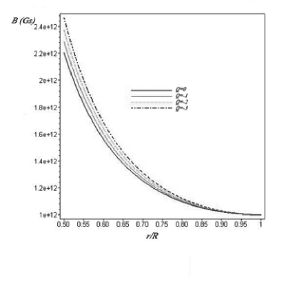
Figure 1: A plot of magnetic field $B$ against $r/R$ in the exterior of a relativistic magnetized compact star with typical parameters, $M=2M_{\odot}$, $R=10~{}km$. The Weyl charges are taken in the unit of $M^{2}$.

The braneworld enhancement of the exterior magnetic field at the surface of the relativistic star is given in table 1 which varies between $2$ and $3$ depending on intensity of Weyl charge selected.

Table 1: The amplification of exterior magnetic field at the boundary surface of a typical relativistic compact star as a result of brane tension. The Newtonian value for the magnetic field at the pole is taken as $B_{0}=10^{12}~{}G$. The mass of star is $M=2M_{\odot}$ and the radius is $R=10~{}km$. The values for Weyl charge $Q$ are taken as usual in unit of $M^{2}$.

${\bf Q}$	-0.5	-1.0	-1.5	-2.0	-2.5	-3.0
${\bf B,~{}(10^{12}~{}G)}$	1.94	2.05	2.17	2.32	2.51	2.77

As can be seen from the presented graphs in figure 2 the magnetic field strength outside the star will be enhanced by braneworld parameter up to approximately $170$ percent compared with that in the flat space-time limit depending on the value of parameter $Q$ selected.

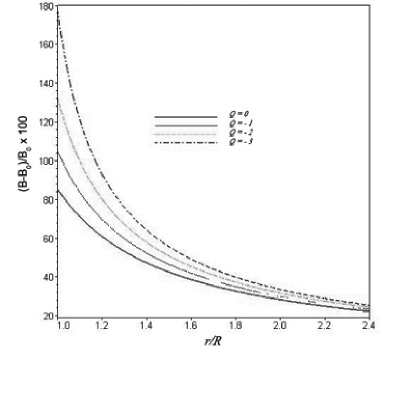
Figure 2: The percentage increase in the magnetic field strength as a function of radial distance $r/R$ in the exterior of relativistic magnetized star depending on Weyl charge $Q$.

III.3 Interior numerical solution

The assumption of constant density of matter is approximately realistic because for non-exotic equations of state bps71 the change in density is only about one order of magnitude within three quarters of the neutron star volume. For uniform density star $(\rho=const)$ one can select that $U=0$ and $P=0$. Then according to the Einstein equations (2)–(5) and Maxwell equations (35)–(36) the equation for unknown radial function will take a form

$$\frac{d}{dr}\left[\frac{\Delta(r)}{\rho+p(r)}\frac{d}{dr}\left(r^{2}F\right)\right]-\frac{2F}{\left[\rho+p(r)\right]\Delta(r)}=0\ ,$$ (49)

where

$$\Delta(r)\equiv\left[1-\frac{2M}{r}\left(\frac{r}{R}\right)^{3}\left[1-\frac{Q}{6MR}\right]\right]^{1/2}\ ,$$ (50)

$$p(r)=\frac{\left[\Delta(r)-\Delta(R)\right]\left(1-Q/3MR\right)\rho}{\left[3\Delta(R)-\Delta(r)\right]-\left[3\Delta(R)-2\Delta(r)\right]Q/3MR}\ ,$$ (51)

$$m(r)=M\left[1-\frac{Q}{6MR}\right]\left(\frac{r}{R}\right)^{3}\ .$$ (52)

For finding the interior numerical solution we have also used the same technique as for the exterior case, i.e the ODE is considered as an initial value problem. For initial value of $B(\overline{r}=1)$ taken the value obtained from the exterior solution due to assumed continuity of magnetic field through the surface of the star. The Maxwell equation is integrated up to $\overline{r}=0.5$ where the existence of the dipolar magnetic field is expected.

Figure 3: A plot of magnetic field $B$ against $r/R$ for the interior region of typical compact relativistic star with parameters $M=2~{}M_{\odot}$, $R=10~{}km$ and $\rho=1.0\times 10^{14}$ g cm^-3 for various values of $Q$. The brown solid curve is for $Q=0$, the red dotted curve for $Q=-1$, the green dashed curve for $Q=-2$ and the blue dot–dashed curve for $Q=-3$ which are taken in the unit of $M^{2}$.

In the figure 3 we present the magnetic field strength of the interior of a star as a function of the radial distance from $\overline{r}=0.5$ (which is normalized on the radius of star $R$) up to the stellar surface $\overline{r}=1$. One can see from the presented graphs the field strength interior of the star will be enhanced by braneworld parameter and at the half radius of the star is increased by up to approximately $20$ percent compared with that for the general-relativistic Schwarzschild star depending on the value of parameter $Q$ selected.

IV Astrophysical Consequences

Assume that the oblique magnetized braneworld star is rotating and $\chi$ is the inclination angle between axis of rotation and magnetic momentum and observed as pulsar through magnetic dipole radiation. Then the luminosity of the relativistic star in the case of a purely dipolar radiation, and the power radiated in the form of dipolar electromagnetic radiation, is given by ra04

$$L_{em}=\frac{\Omega^{4}_{{}_{R}}R^{6}{\widetilde{B}}^{2}_{0}}{6c^{3}}\sin^{2}\chi\ ,$$ (53)

where subscript $0$ denotes the value at $r=R$.

When compared with the equivalent Newtonian expression for the rate of electromagnetic energy loss through dipolar radiation ll87

$$(L_{em})_{\rm Newt}=\frac{\Omega^{4}R^{6}B_{0}^{2}}{6c^{3}}\sin^{2}\chi\ ,$$ (54)

it is easy to realize that the general relativistic braneworld corrections emerging in expression (53) are partly due to the magnetic field amplification ${\widetilde{B}}_{0}=F_{{}_{R}}B_{0}$ at the stellar surface and partly to the increase in the effective rotational angular velocity produced by the gravitational redshift as $\Omega=\Omega_{{}_{R}}A_{{}_{R}}$.

The presence of a braneworld tension has the effect of enhancing the rate of energy loss through dipolar electromagnetic radiation by an amount which can be easily estimated to be

$$\frac{L_{em}}{(L_{em})_{{}_{\rm Newt}}}=\left(\frac{F_{{}_{R}}}{A^{2}_{{}_{R}}}\right)^{2}\ ,$$ (55)

and whose dependence is shown in figure 4 with a solid line. Considering expression (53) in the selected range for the brane tension, it is straightforward to realize that the Newtonian expression (54) underestimates the electromagnetic radiation losses of a factor which may reach few hundreds depending on the value of the brane tension parameter.

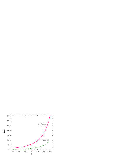
Figure 4: General relativistic amplification of the energy loss through dipolar electromagnetic radiation as a function of absolute value of Weyl charge. The solid line refers to the ratio of energy loss in the braneworld with energy loss in the flat spacetime, while dashed line is with energy loss in the Schwarzschild curvature background. It is shown with a dashed line for comparison. Weyl charge $|Q|$ in abscissa is taken in the unit of $M^{2}$.

In the figure 5 we present enhancement of the electromagnetic energy loss by brane tension depending on compactness of the relativistic star and prove that the braneworld effects are more important for ultracompact stars.

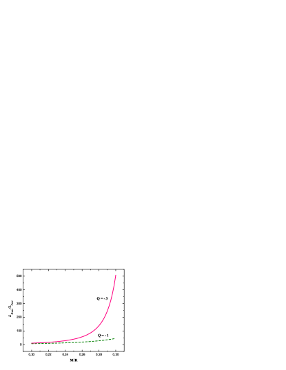
Figure 5: General relativistic amplification of the energy loss through dipolar electromagnetic radiation as a function of stellar compactness $M/R$ for different Weyl charges.

Expression (53) could be used to investigate the rotational evolution of magnetized neutron stars with predominant dipolar magnetic field anchored in the crust which converting its rotational energy into electromagnetic radiation. A detailed investigation of general relativistic effects for Schwarzschild stars has already been performed by Page et al. pgz00 , who have paid special attention to the general relativistic corrections that need to be included for a correct modeling of the thermal evolution but also of the magnetic and rotational evolution. It should be remarked, however, that in their treatment Page et al. pgz00 have taken into account the general relativistic amplification of magnetic field due to the curved background spacetime, but did not include the corrections due to the gravitational redshift. As a result, the general relativistic electromagnetic luminosity estimated by Page et al. pgz00 is smaller than the one computed in our paper ra04 where all general relativistic effects are taken into account.

V Conclusion

We have studied the stationary magnetic field of isolated relativistic compact star in the braneworld assuming that their magnetic fields are confined to the stellar crust of ideal perfect matter and have been working with the braneworld effects on the stellar magnetic field, accompanied by proper boundary conditions. In other words we generalized the general relativistic approach in the sense that we took into account the effect of additional braneworld tension on electromagnetic fields.

First we have solved interior Maxwell equations analytically and found exact solution for interior magnetic field inside the stellar stiff matter with unrealistic equation of state.

Then we have found numerical calculations which take into account the effect of brane tension on the structure of magnetic field outside the star and configuration of interior magnetic field for the stellar matter with constant density. Comparing the behaviour of the magnetic field when brane tension effects are included with the case when they are neglected, one can see enhancement of magnetic field especially near the surface of the relativistic star for external field and in the inner boundary taken for the interior field. This effect is stronger the more bigger the braneworld parameter $Q$ is.

Numerically calculated magnetic field structure for the external magnetic field, without brane tension effects incorporated, totally match the known analytical solution for magnetic field when ’branetension charge’ $Q$ is equal to zero.

The numerical calculations made confirm that there are two effects of brane tension on magneto-dipolar emission. One is due to amplification of surface magnetic field by brane tension. Other is due to the presence of function $Q/r^{2}$ in the red-shift factor $\sqrt{1-2M/r+Q/r^{2}}$ defined at the stellar surface in the expression for power of magnetodipolar radiation. We have found that the effect of branetension on magnetic fields of compact stars can be very important, and the expression for magnitodipolar luminosity of rotating braneworld magnetized star gives enhancement up to two orders.

While the previous papers extensively studied the influence of braneworld effects into the different astrophysical processes and cosmological problems, we conclude here the incorporation of the brane tension effect into magnetic field structure of the relativistic stars, could give an additional key for astrophysical evidence of the parameter $Q$.

References

- (1) R. C. Duncan, C. Thompson, Astrophys. J., 392, L9 (1992).
- (2) C. Thompson, R. C. Duncan, Mon. Not. R. Astron. Soc., 275, 255 (1995).
- (3) A. S. Majumdar, N. Mukherjee, Int. J. Mod. Phys. D, 14, 1095 (2005).
- (4) S. Creek, R. Gregory, P. Kanti, B. Mistry, hep-th/0606006 (2006).
- (5) R. Maartens, Living Rev. Relativity, 7, 7 (2004).
- (6) C. Germany, R. Maartens, Phys. Rev. D, 64, 124010 (2001).
- (7) N. K. Dadhich, R. Maartens, P. Papodopoulos, V. Rezania, Phys. Lett. B, 487, 1 (2000).
- (8) C. R. Keeton, Phys. Rev. D., 73, 104032 (2006).
- (9) C. R. Keeton, A. O. Petters, Phys. Rev. D., 72, 104006 (2005).
- (10) C. R. Keeton, A. O. Petters, Phys. Rev. D., 73, 044024 (2006).
- (11) L. Iorio, gr-qc/0504053 (2005).
- (12) A. J., Deutsch, Ann. Astrophys., 1, 1 (1955).
- (13) R. Ruffini, A. Treves, Astrophys. Lett., 13, 109 (1973).
- (14) V. L. Ginzburg, L. M. Ozernoy, Zh. Eksp. Teor. Fiz., 47, 1030 (1964).
- (15) J. L. Anderson, J. M. Cohen, Astrophys. Space Science, 9, 146 (1970).
- (16) J. A. Petterson, Phys. Rev., D, 10, 3166 (1974).
- (17) I. Wasserman, S. L. Shapiro, Astrophys. J., 265, 1036 (1983).
- (18) A. Muslimov, A. K. Harding, Astrophys. J., 485, 735 (1997).
- (19) A. Muslimov, A. I. Tsygan, Mon. Not. R. Astron. Soc., 255, 61 (1992).
- (20) L. Rezzolla, B. J. Ahmedov, J. C. Miller, Mon. Not. R. Astron. Soc., 322, 723 (2001a); Erratum 338, 816 (2003).
- (21) L. Rezzolla, B. J. Ahmedov, J. C. Miller, Found. Phys., 31, 1051 (2001b).
- (22) L. Rezzolla, B. J. Ahmedov, Mon. Not. R. Astron. Soc., 352, 1161 (2004).
- (23) Y. Kojima, N. Matsunaga, T. Okita, Mon. Not. R. Astron. Soc., 348, Issue 4, 1388 (2004).
- (24) A. Gupta, A. Mishra, H. Mishra, A. R. Prasanna, Class. Quantum Grav. 15, 3131 (1998).
- (25) A. R. Prasanna, A. Gupta, Nuovo Cimento B, 112, 1089 (1997).
- (26) U. Geppert, D. Page, T. Zannias, Phys. Rev. D, 61, 123004 (2000).
- (27) D. Page, U. Geppert, T. Zannias, Astron. Astrophys., 360, 1052 (2000).
- (28) O. Zanotti, L. Rezzolla, Mon. Not. R. Astron. Soc. 331, 376 (2002).
- (29) R. C. Tolmann, Phys. Rev., 55, 364 (1939).
- (30) J. R. Oppenheimer, G. M. Volkoff, Phys. Rev., 55, 374 (1939).
- (31) N. K. Glendenning, Compact Stars, Springer-Verlag, New York (1996).
- (32) G. Baym, C. Pethick, P. Sutherland, Astrophys. J., 170, 299 (1971).
- (33) G. B. Arfken, H. J. Weber, Mathematical Methods for Physicists, 5th edn. Academic Press, San Diego (2001).
- (34) W. H. Press, B. P. Flannery, S. A. Teukolsky, W. T. Vetterling, Numerical Recipes: The Art of Scientific Computing (Fortran Version), Cambridge University Press, Cambridge (1989).
- (35) L. D. Landau, E. M. Lifshitz, The Classical Theory of Fields, Pergamon, Oxford (1987).