Application of Discrete Differential Forms to Spherically Symmetric Systems in General Relativity

Abstract.

In this article we describe applications of Discrete Differential Forms in computational GR. In particular we consider the initial value problem in vacuum space-times that are spherically symmetric. The motivation to investigate this method is mainly its manifest coordinate independence. Three numerical schemes are introduced, the results of which are compared with the corresponding analytic solutions. The error of two schemes converges quadratically to zero. For one scheme the errors depend strongly on the initial data.

1. Introduction

Most methods that are presently used in numerical GR are in some sense referred to a coordinate system. This can be a major problem, because not only is it impossible in general to cover a global space-time with a single coordinate chart. But also it is generally impossible to know beforehand the effects that certain gauge conditions specified during the course of a simulation will imply.

In view of this the question occurs, as to whether it is possible to develop a numerical method that is manifestly coordinate invariant. One such method is Regge calculus [1] which, unfortunately, so far has not played a role in computational GR (see however [2]). In other approaches to treat the problem of coordinate dependencies multiple coordinate systems are used to cover the space-time [3, 4, 5].

However, a manifestly invariant numerical method must be based on invariant quantities describing the geometry of space-time. The prime examples for invariant quantities on a manifold are the scalar fields, but in the usual description even they are coordinate dependent, because the description of the points of the manifold themselves depends on the choice of a coordinate system. Therefore, in order to avoid coordinates we must not even use coordinates for the localisation of points of the space-time manifold. This implies that we cannot use the usual definition of a manifold as a collection of coordinate charts with transition functions which is the basis of almost all analytical and numerical treatments of the Einstein equations.

In the usual procedure for discretisation the manifold structure is untouched while the equations are discretised, i.e., evaluated only for a finite number of points of the manifold. When the use of coordinates is to be avoided one has to start the discretisation at an even lower level namely on that of the manifold itself. Hence, on a quite basic level the space-time can be considered as a collection of abstract objects called points. The structures on the space-time are then described as certain relations between these points. In our case the relevant structure consists of primarily topological and geometric relationships. For the present purpose we find it more reasonable to consider the topological relationships as given in advance so that the aim of computational GR is to find the geometric relations between the points based on an appropriate formulation of the Einstein equations.

To achieve this we continue the work presented in [6]. That is we approximate a manifold and its differentiable structure by a cellular paving [7], i.e. a collection of finitely many cells. The cells are the images of a certain number of standard shapes like (hyper-)cubes or $n$-simplices. In the case where all standard shapes are simplices we talk about a triangulation and the cellular paving is a simplicial complex. The cellular paving is supposed to have the same topological properties as the envisaged space-time.

To illustrate the idea we consider the example of a standard 3-simplex which can be viewed as the interior of a tetrahedron. It is a 3-dimensional manifold. Its boundary is composed of four 2-simplices (faces), six 1-simplices (edges) and four 0-simplices (nodes). With such $p$-simplices we can associate several quantities which can be interpreted in a physical way. Examples are the charge inside a volume, a flux through a face, the work done along an edge or the value of a potential at a given point. In all these cases we associate numbers with a simplex and these numbers are usually obtained by integration, i.e., by adding up contributions from ‘infinitesimal’ pieces making up the finite simplex. So, in each case we obtain a map from $p$-simplices to numbers.

Differential $p$-forms can be viewed as ‘the objects which are integrated over $p$-dimensional submanifolds’ so they provide maps from $p$-dimensional submanifolds to the reals. Thus, the maps presented above correspond to differential forms, but restricted to $p$-simplices. These objects are known as discrete differential forms. They have received some attention since Bossavit [8] had pointed out that they correspond to the lowest order mixed finite element spaces defined by Nédélec [9] (see also [10]). Finite elements of mixed type have been used successfully in numerical applications to electrodynamics, see [7, 11, 12]. In numerical GR the finite element method is used e.g. in [13].

Our task is now to relate geometric properties such as lengths, angles, holonomies and curvature using differential forms to the triangulation and the various parts of the simplices respectively. Since $0$-forms are functions they describe properties at single points. In order to formulate relations between points such as the distance between two points or the holonomy around a loop we need $p$-forms with $p>0$.

In order to use this approach one needs to have a formulation of geometries and, in particular, of GR which uses differential forms. A formulation of geometries based on differential forms has been provided by É. Cartan [14]. The further step towards a formulation of GR using differential forms has been carried out by several authors. We mention here the work of Sparling [15] who has set up an exterior differential system of equations which is closed if and only if the vacuum Einstein equations hold. In [6] we have shown in detail how to set up the discrete formalism based on this exterior system using the ideas explained above.

In summary, the variables of our proposed discrete formulation will be the integrals of differential forms over submanifolds. In order to get a finite number of variables we use a finite number of these submanifolds based on a triangulation of the computational domain and discretise a description of GR that uses (finitely many) differential forms.

The formulation of GR that we use is based on the Cartan formalism of moving frames and Sparling’s exterior system for vacuum GR. In this article we describe a simplification of the general formalism which occurs in spherical symmetry. The plan of the paper is as follows. In sect. 2 we describe the equations which result from a symmetry reduction. In section 3 we present three possibilities to implement these equations in a fully discrete evolution scheme. In section 4 we discuss how the method can be tested and in section 5 we present the results of those tests. Some final remarks can be found in section 6.

2. The spherically symmetric equations

We start with the formulation of GR using exterior forms [15]. The basic variables in this formalism are the four 1-forms of a pseudo-orthonormal tetrad $\boldsymbol{\theta}^{i}$, $i=0,\ldots,3$ [16]. Together with the coefficients $\eta_{ik}=\text{diag}(1,-1,-1,-1)$ they define the metric as

(1) $$g=\boldsymbol{\theta}^{0}\otimes\boldsymbol{\theta}^{0}-\boldsymbol{\theta}^{1}\otimes\boldsymbol{\theta}^{1}-\boldsymbol{\theta}^{2}\otimes\boldsymbol{\theta}^{2}-\boldsymbol{\theta}^{3}\otimes\boldsymbol{\theta}^{3}=\eta_{ik}\boldsymbol{\theta}^{i}\otimes\boldsymbol{\theta}^{k}.$$

For the description of the connection in this formalism sixteen 1-forms ${\boldsymbol{\omega}^{i}}_{k}$, $i,k=0,\ldots,3$ are used. The connection should be compatible with the metric and torsion free, which translates into the antisymmetry requirement and the first Cartan equation, respectively:

(2) $$\eta_{ik}{\boldsymbol{\omega}^{k}}_{j}+\eta_{jk}{\boldsymbol{\omega}^{k}}_{i} =0, \mathbf{d}\boldsymbol{\theta}^{i}+{\boldsymbol{\omega}^{i}}_{k}\boldsymbol{\theta}^{k} =0.$$

Furthermore the metric should fulfil Einstein’s field equations, which is equivalent to

(3) $$\mathbf{dL}_{i}=\mathbf{S}_{i}+8\pi{T_{i}}^{k}\boldsymbol{\Sigma}_{k}.$$

Here, $T_{ik}$ is the usual energy momentum tensor and

$$\boldsymbol{\Sigma}_{i}=\frac{1}{6}\varepsilon_{ijkl}\boldsymbol{\theta}^{j}\boldsymbol{\theta}^{k}\boldsymbol{\theta}^{l},$$

are the so called hypersurface 3-forms. The forms $\mathbf{L}_{i}$ and $\mathbf{S}_{i}$ are the Nester-Witten 2-form and the Sparling 3-form, defined by (see [6, 15]):

(4) $$\mathbf{L}_{i} =\frac{1}{2}\varepsilon_{ijkl}{\boldsymbol{\omega}^{jk}}\boldsymbol{\theta}^{l}, \mathbf{S}_{i} =\frac{1}{2}\varepsilon_{ijkl}\left(\boldsymbol{\omega}^{jk}{\boldsymbol{\omega}^{l}}_{m}\boldsymbol{\theta}^{m}-{\boldsymbol{\omega}^{j}}_{m}\boldsymbol{\omega}^{mk}\boldsymbol{\theta}^{l}\right).$$

In vacuum, when ${T_{i}}^{k}=0$, these equations determine the geometry of space-time. If there is matter, additional matter equations are needed. However, we will be concerned only with the vacuum case so that we will have to solve the equations

(5a) $$\mathbf{d}\boldsymbol{\theta}^{i}+{\boldsymbol{\omega}^{i}}_{k}\boldsymbol{\theta}^{k} =0,$$

(5b) $$\mathbf{dL}_{i} =\mathbf{S}_{i}.$$

Although the geometry is fixed, there is still the freedom of choosing a gauge, i.e. there are Lorentz transformations $\Lambda^{i}{}_{k}$ of the tetrad that do not change the metric

(6) $$g=\eta_{ik}\boldsymbol{\theta}^{i}\otimes\boldsymbol{\theta}^{k}=\eta_{ik}{\Lambda^{i}}_{j}\boldsymbol{\theta}^{j}\otimes{\Lambda^{k}}_{l}\boldsymbol{\theta}^{l}=(\eta_{ik}\Lambda^{i}{}_{j}\Lambda^{k}{}_{l})\,\boldsymbol{\theta}^{j}\otimes\boldsymbol{\theta}^{l}.$$

That means by using the tetrad for the description of geometries we introduced unphysical (gauge) degrees of freedom. The same problem occurs when coordinate systems are used. However, we believe that the tetrad, beeing a geometric object, has a more intuitive meaning than mere coordinates. Therefore, it might be easier to choose a useful tetrad than an appropriate coordinate system.

In this work we will concentrate on general relativistic systems with spherical symmetry. Thus, we will assume that the rotation group $SO(3)$ acts isometrically on the space-time and that the orbits of this action are 2-dimensional space-like submanifolds. These are necessarily spheres whose area we write as $4\pi R^{2}$. In appendices A and B it is shown, how to ‘factor out’ the symmetry action i.e., the angular dependence and how to derive an exterior system on the 2-dimensional ‘orbit space’ ${\mathcal{M}}_{1}$ spanned by the radial and the time directions.

This can be done by a decomposition of the 4-dimensional space-time manifold into the 2-dimensional spheres and the 2-dimensional orbit space, followed by some simplifications and results in the following system

(7a) $$0 =\mathbf{d}f_{0}-f_{1}\boldsymbol{\omega}-\frac{1}{2}\left(f_{1}^{2}-3f_{0}^{2}-\frac{1}{R^{2}}\right)\boldsymbol{\theta}^{0}+(f_{0}f_{1})\,\boldsymbol{\theta}^{1},$$

(7b) $$0 =\mathbf{d}f_{1}-f_{0}\boldsymbol{\omega}-\frac{1}{2}\left(f_{0}^{2}-3f_{1}^{2}+\frac{1}{R^{2}}\right)\boldsymbol{\theta}^{1}+(f_{0}f_{1})\,\boldsymbol{\theta}^{0},$$

(7c) $$0 =\mathbf{d}\left(\sqrt{R^{2}}\left(R^{2}f_{0}^{2}-R^{2}f_{1}^{2}+1\right)\right),$$

(7d) $$0 =f_{0}\left(\mathbf{d}\boldsymbol{\theta}^{1}+{\boldsymbol{\omega}}\boldsymbol{\theta}^{0}\right)-f_{1}\left(\mathbf{d}\boldsymbol{\theta}^{0}+{\boldsymbol{\omega}}\boldsymbol{\theta}^{1}\right).$$

Here $(\boldsymbol{\theta}^{0},\boldsymbol{\theta}^{1})$ is a dyad in the 2-dimensional orbit space ${\mathcal{M}}_{1}$ which carries a Lorentzian metric. The $SO(1,1)$ connection on this space is given by the 1-form ${\boldsymbol{\omega}}$. It is a consequence of the equations above that this connection is torsion free. The geometric properties of the orbits are described by the functions $f_{0}$, $f_{1}$ and $R^{2}$ (e.g. $4\pi R^{2}$ is the area of the orbit). For details see appendix A.

By introducing the 1-forms

(8) $$\tilde{\boldsymbol{\theta}}^{0} :=\frac{1}{R}\boldsymbol{\theta}^{0}, \tilde{\boldsymbol{\theta}}^{1} :=\frac{1}{R}\boldsymbol{\theta}^{1},$$

$${\boldsymbol{\alpha}} :=f_{0}\boldsymbol{\theta}^{0}+f_{1}\boldsymbol{\theta}^{1}, {\boldsymbol{\beta}} :=f_{1}\boldsymbol{\theta}^{0}+f_{0}\boldsymbol{\theta}^{1}$$

the equations (7) can be rewritten as follows

(9a) $$\mathbf{d}\tilde{\boldsymbol{\theta}}^{0}+{\boldsymbol{\omega}}\tilde{\boldsymbol{\theta}}^{1}+\boldsymbol{\alpha}\tilde{\boldsymbol{\theta}}^{0} =0,$$

(9b) $$\mathbf{d}\tilde{\boldsymbol{\theta}}^{1}+{\boldsymbol{\omega}}\tilde{\boldsymbol{\theta}}^{0}+\boldsymbol{\alpha}\tilde{\boldsymbol{\theta}}^{1} =0,$$

(9c) $$\mathbf{d}\boldsymbol{\alpha} =0,$$

(9d) $$\mathbf{d}\boldsymbol{\beta}+2\boldsymbol{\alpha}\boldsymbol{\beta}+\tilde{\boldsymbol{\theta}}^{0}\tilde{\boldsymbol{\theta}}^{1} =0,$$

(9e) $$\mathbf{d}{\boldsymbol{\omega}}-\boldsymbol{\alpha}\boldsymbol{\beta}-\tilde{\boldsymbol{\theta}}^{0}\tilde{\boldsymbol{\theta}}^{1} =0,$$

together with the algebraic relations

(10) $$\boldsymbol{\alpha}\tilde{\boldsymbol{\theta}}^{0}+\boldsymbol{\beta}\tilde{\boldsymbol{\theta}}^{1}=0,\qquad\boldsymbol{\alpha}\tilde{\boldsymbol{\theta}}^{1}+\boldsymbol{\beta}\tilde{\boldsymbol{\theta}}^{0}=0.$$

The two equations (10) are needed to ensure that $\boldsymbol{\alpha}$ and $\boldsymbol{\beta}$ are constructed out of only two functions. They can be interpreted as

(11) $$\star\boldsymbol{\alpha}=\boldsymbol{\beta}$$

where $\star$ is the 2-dimensional Hodge operator [17]. In the calculations we will use discrete versions of both (10) and (11).

From the definition of the Hodge operator it is clear, that $\star\boldsymbol{\theta}^{1}=\boldsymbol{\theta}^{0}$. This means that in (9) we have actually only three 1-forms $\boldsymbol{\alpha}$, $\boldsymbol{\theta}^{1}$ and ${\boldsymbol{\omega}}$ and their Hodge duals. From now on the Hodge duals will be called dual forms, whereas the forms $\boldsymbol{\alpha}$, $\boldsymbol{\theta}^{1}$ and $\boldsymbol{\omega}$ themselves get the generic name direct forms. We also have for every form and its Hodge dual an equation, where its exterior derivative is involved except for the dual of ${\boldsymbol{\omega}}$. It turns out, that the exterior derivative of this form is pure gauge because it can be set to any value by an appropriate choice of gauge in ${\mathcal{M}}_{1}$. This property can be used to fix the gauge.

If the geometry is regular at the origin ($R=0$) then we may also include it into the computational domain. Thus, the origin becomes a boundary. We choose the gauge such that the dyad at the origin can be defined as the limit of $(\boldsymbol{\theta}^{0},\boldsymbol{\theta}^{1})$, i.e. such that this limit exists.

Then it is easy to verify that if we choose at $R=0$ an arbitrary vector $\mathbf{V}=V^{0}\mathbf{e}_{0}+V^{1}\mathbf{e}_{1}$ with finite components $(V_{0},V_{1})$, then $\mathbf{d}R^{2}(\mathbf{V})=0$ and $\mathbf{d}R(\mathbf{V})=V_{R}<\infty$. It follows from (62) that in the limit $R\rightarrow 0$ the expression $R(f_{0}\boldsymbol{\theta}^{0}+f_{1}\boldsymbol{\theta}^{1})(\mathbf{V})$ must be finite. It is clear that $R\boldsymbol{\theta}^{0}(\mathbf{V})=0$ and $R\boldsymbol{\theta}^{1}(\mathbf{V})=0$ at $R=0$. Thus, the limits of $Rf_{0}$ and $Rf_{1}$ must be finite there, and hence $f_{0}$ and $f_{1}$ diverge. That means we must use the variables $\tilde{f}_{0}:=Rf_{0}$ and $\tilde{f}_{1}:=Rf_{1}$ instead of $f_{0}$ and $f_{1}$.

Now we insert this observation into the equation (7c), or rather into its solution

(12) $$R(\tilde{f}_{0}^{2}-\tilde{f}_{1}^{2}+1)=\mbox{const.}$$

Since $\tilde{f}_{0}$ and $\tilde{f}_{1}$ are finite, it follows that the constant vanishes. It turns out that in general this constant is twice the mass of the black hole, and thus the limit $R\rightarrow 0$ only exists for the flat geometry. In this case one may easily rewrite (7) and (9)-(11) such that the variables are $\tilde{f}_{0}$, $\tilde{f}_{1}$, $\tilde{\boldsymbol{\alpha}}:=R\boldsymbol{\alpha}$, $\tilde{\boldsymbol{\beta}}:=R\boldsymbol{\beta}$, $\boldsymbol{\theta}^{0}$, $\boldsymbol{\theta}^{1}$ and $\boldsymbol{\omega}$.

We are now in a position to apply the discretisation procedure as explained in [7]. However, the situation in GR is significantly different from electrodynamics so that there is no straightforward implementation. For one thing the distinction between direct and dual forms is used in electrodynamics in an elegant way by employing a dual mesh. It is not so clear whether one can make use of this also in GR, because the description of dual forms on the dual mesh strongly relies on the Euclidean character of the metric. Consequently in electrodynamics one only discretises space using the method of discrete differential forms while we aim at fully discrete schemes.

Furthermore, electrodynamics is a linear theory while the nonlinearity of GR is apparent from the appearance of the wedge product which has to be implemented on the discrete level. So we cannot simply adapt the implementation of electrodynamics, but we will have to look at the forms differently. The aim is to split a possibly large system of nonlinear equations into many small systems of equations in order to get one independent system for every simplex. How this is done in practice, is described in [6] and briefly in the following section.

3. Implementation of the discrete equations

In section 2 and appendix A we derived systems of exterior equations on ${\mathcal{M}}_{1}$. Now we present methods for discretising them and develop numerical schemes. Since there is no unique natural way, we use different discretisation schemes to explore various possibilities. The first scheme will be based on the system (7), the second one is obtained through a discretisation of the equations (9),(10) and to get the third scheme we discretise the system (9),(11).

3.1. Application of Whitney forms

As indicated in the introduction, we approximate the manifold by taking into account finitely many of its subsets. Moreover we want to use discrete differential forms as an approximation for the continuous differential forms.

It is known that the opposite, i.e. the extension of a discrete differential form to a continuous differential form can be done with the help of the so-called Whitney forms [18]. These are a special class of forms which can be used to construct continuous forms from discrete forms. However, they can exist only on special domains such as simplices, $n$-dimensional cubes and shapes, that can be constructed from a cube by collapsing some of its edges [19] such as pyramids or prisms. The numerical variables are then the integrals of the forms over the corresponding figures.

We have chosen the first possibility, i.e. we are searching for an approximation of space-time by taking subsets into account, that can be continuously mapped to simplices. In the 2-dimensional case these simplices are nodes, edges and faces. The reason for this choice is, that for other shapes it is not possible to get an exterior product from (anti-)symmetry requirements alone. This leads to anaesthetic ambiguities, and since the exterior product of Whitney forms is in general not a Whitney form, symmetry assumptions are the best way to introduce the discrete exterior product.

Using simplices one gets, up to a normalisation, an exterior product essentially from the following requirements

1. The discrete exterior product fulfils the usual commutation rule for forms, i.e. for a $p$-form $\boldsymbol{\alpha}^{p}$ and a $q$-form $\boldsymbol{\beta}^{q}$ we have

   $$\boldsymbol{\alpha}^{p}\wedge\boldsymbol{\beta}^{q}=(-1)^{pq}\boldsymbol{\beta}^{q}\wedge\boldsymbol{\alpha}^{p}.$$

2. When the orientation of the simplex is changed, the sign of the corresponding value of the discrete exterior product changes. The same is true for every Discrete Differential Form.

These requirements lead almost immediately to the following formula for the discrete exterior product between 1-forms $\boldsymbol{\alpha}$ and $\boldsymbol{\beta}$

(13) $$\boldsymbol{\alpha}\boldsymbol{\beta}[n_{0},n_{1},n_{2}] =\frac{1}{6}\big{(}\boldsymbol{\alpha}[n_{0},n_{1}]\boldsymbol{\beta}[n_{0},n_{2}]-\boldsymbol{\alpha}[n_{0},n_{2}]\boldsymbol{\beta}[n_{0},n_{1}]$$

$$\qquad+\boldsymbol{\alpha}[n_{1},n_{2}]\boldsymbol{\beta}[n_{1},n_{0}]-\boldsymbol{\alpha}[n_{1},n_{0}]\boldsymbol{\beta}[n_{1},n_{2}]$$

$$\qquad+\boldsymbol{\alpha}[n_{2},n_{0}]\boldsymbol{\beta}[n_{2},n_{1}]-\boldsymbol{\alpha}[n_{2},n_{1}]\boldsymbol{\beta}[n_{2},n_{0}]\big{)},$$

where the expression $\boldsymbol{\gamma}[n_{0},\ldots,n_{p}]$ is the numerical variable corresponding to the integral of the $p$-form $\boldsymbol{\gamma}$ over the simplex with nodes $\{n_{0},\ldots,n_{p}\}$ and orientation given by the ordered tuple of vectors $(n_{1}-n_{0},\ldots,n_{p}-n_{0})$. It turns out that this definition and its analogues for higher degree forms yield an algebraic structure which is not associative in contrast to the continuous case. How this non-associativity influences the method is not clear. It is clear however, that the terms which become ambiguous due to the non-associativity are of higher order so they converge to zero faster in the continuum limit.

For the discretisation of the exterior derivative, we remember Stokes theorem and get for a 1-form $\boldsymbol{\alpha}$

(14) $$\mathbf{d}\boldsymbol{\alpha}[n_{0},n_{1},n_{2}]=\boldsymbol{\alpha}[n_{1},n_{2}]-\boldsymbol{\alpha}[n_{0},n_{2}]+\boldsymbol{\alpha}[n_{0},n_{1}].$$

Figure 1. The boundary of the 2-dimensional oriented face $[n_{0},n_{1},n_{2}]$ is composed of three oriented edges $[n_{0},n_{1}]$, $[n_{0},n_{2}]$, $[n_{1},n_{2}]$ and three nodes $n_{0}$, $n_{1}$, $n_{2}$.

3.2. Properties of the simplicial mesh

Now we come to the numerical schemes. Common to all three schemes is the way of generating a simplicial approximation of a subset of ${\mathcal{M}}_{1}$. We start from appropriate initial data. That means from somewhere we have a 1-dimensional simplicial complex $\mathcal{C}_{i}$ [20], that approximates a space-like curve in ${\mathcal{M}}_{1}$ (see section 4 for details). At each node of $\mathcal{C}_{i}$ two linearly independent light-like directions $\mathbf{l}_{0}$ and $\mathbf{l}_{1}$ exist. It is clear, that a light-like curve with tangent-vector $\mathbf{l}_{0}$ at a node $n_{0}$ will have an intersection with a light-like curve with tangent vector $\mathbf{l}_{1}$ at another node $n_{1}$. To create a face of the mesh, that contains an edge of $\mathcal{C}_{i}$, we require the two missing edges to be approximations of these light-like curves. Their intersection becomes the new node $n_{2}$. For obvious reasons, these faces are called upwards directed.

This construction seems to be the simplest invariant method to define the position of $n_{2}$ in $(1+1)$-dimensional manifolds. It is a geometric construction and can be generalised to higher dimensions. The choice of the nodes at a later time and their connections to the nodes at the initial time is essentially arbitrary and only restricted by topological considerations. It is only when the $\boldsymbol{\theta}^{i}$ are known on all the edges that the geometry of the mesh is determined. We will see later that a part of these values can be specified freely while the rest is determined from the equations.

As in all numerical simulations degeneracies may occur. For instance two adjacent nodes in the same level may have a time-like distance. However, this must be seen as a sign that the mesh is too coarse and should be refined.

The other type of faces is called downwards directed, and is created by joining the intersections of the light-like curves in adjacent upwards directed faces. When $\mathcal{C}_{i}$ has $n$ edges, we now have $n$ upwards directed and $(n-1)$ downwards directed faces. The collection of these faces will be called the first time-step.

Obviously, this procedure can be continued by taking the collection of the non light-like edges of the downwards directed faces as a new initial complex $\mathcal{C}^{\prime}_{i}$, until the intersection of the light-like curves from the boundary of $\mathcal{C}_{i}$ is reached. That means that we calculate the domain of dependence of $\mathcal{C}_{i}$. In principle we could have implemented boundary conditions, but we wanted to concentrate on the time evolution scheme and periodic boundary conditions are not possible in spherical symmetry. Figure 2 shows the triangulation.

Figure 2. The triangulation of the domain of dependence of $\mathcal{C}_{i}$.

Having a simplicial mesh, the exterior product and derivative, we can now take care of the discrete equations.

In what follows we will present three numerical schemes. Common to all schemes is that for each triangle a system of equation has to be solved. These are coupled non-linear algebraic equations. Their analysis is somewhat complicated and their status is not yet clear. They might not have a unique solution. However, at least one solution can be found by Newton’s iteration method. We used the GNU Scientific Library, especially the implementation of a root finding algorithm called modified Powell method by the developers [21, 22].

3.3. Scheme I

For the first scheme the system (7) is used. The variables are the discrete 1-forms $\boldsymbol{\theta}^{0}$, $\boldsymbol{\theta}^{1}$ and $\boldsymbol{\omega}$ as well as the discrete 0-forms $f_{0}$, $f_{1}$ and $R^{-2}$. For the upwards directed faces the numbers

$$\{f_{0}[n_{0}],f_{0}[n_{1}],f_{1}[n_{0}],f_{1}[n_{1}],R^{-2}[n_{0}],R^{-2}[n_{1}],\boldsymbol{\theta}^{0}[n_{0},n_{1}],\boldsymbol{\theta}^{1}[n_{0},n_{1}],\boldsymbol{\omega}[n_{0},n_{1}]\}$$

are given initial data, and

$$\{ f_{0}[n_{2}],f_{1}[n_{2}],R^{-2}[n_{2}],$$

$$\boldsymbol{\theta}^{0}[n_{0},n_{2}],\boldsymbol{\theta}^{0}[n_{1},n_{2}],\boldsymbol{\theta}^{1}[n_{0},n_{2}],\boldsymbol{\theta}^{1}[n_{1},n_{2}],\boldsymbol{\omega}[n_{0},n_{2}],\boldsymbol{\omega}[n_{1},n_{2}]\}$$

are the unknowns.

The equation (7c) is the statement that the function

(15) $$F:=\left(f_{0}^{2}-f_{1}^{2}+R^{-2}\right)/\left(R^{-2}\right)^{3/2}$$

is constant on $\mathcal{M}_{1}$, and it is implemented in this way. Thus, we calculate the constant $C:=F[n_{0}]$ from the (known) values $f_{0}[n_{0}]$, $f_{1}[n_{0}]$ and $R^{-2}[n_{0}]$ and then require

(16) $$F[n_{2}]=\left(\left(f_{0}^{2}-f_{1}^{2}+R^{-2}\right)/\left(R^{-2}\right)^{3/2}\right)[n_{2}]=C,$$

since equation (7c) implies that $F[n_{0}]=F[n_{1}]=F[n_{2}]=C$.

Therefore, the number of equations is six (two 1-form equations for the two light-like edges, one 2-form equation and (16)), but the number of unknowns is nine. We eliminate two unknowns by using the definition of the position of $n_{2}$ (see section 3.2). We get

(17) $$(\boldsymbol{\theta}^{0}-\boldsymbol{\theta}^{1})[n_{0},n_{2}] =0, (\boldsymbol{\theta}^{0}+\boldsymbol{\theta}^{1})[n_{1},n_{2}] =0,$$

expressing the fact that the edges are null.

What remains is the freedom of choosing a gauge. This corresponds to the choice of a cobasis at $n_{2}$. The dyad at $n_{2}$ can be obtained from parallel transport of $\{\boldsymbol{\theta}^{0},\boldsymbol{\theta}^{1}\}$ from the initial hypersurface to $n_{2}$ along an edge. Since parallel transport is defined by $\boldsymbol{\omega}$ we choose it such that

(18) $$\boldsymbol{\omega}[n_{0},n_{2}] =0.$$

The reason to choose this gauge condition is of course that it is the most simple one. Clearly, in general it is the aim to choose the gauge in some sense ‘optimal’, in order to get good results. However, until now we do not understand well, what ‘optimal’ means here. Probably this may become clear once the properties of the equations are better understood.

In the continuum limit (18) corresponds to a dyad that is obtained through parallely transporting the (known) basis at the initial hypersurface along the light-like curves with tangent vector $(\mathbf{e}_{0}+\mathbf{e}_{1})$. This fixes the so-called strong conformal geometry of the null-hypersurface generated by the spherical family of light rays (see Penrose [23]).

For the downwards directed faces the situation is easier. The 0-form equation (16) is automatically fulfilled at all nodes, and the 1-form equations (7a) and (7b) are fulfilled at the light-like edges. What remains are two 1-form equations (7a), (7b) and one 2-form equation (7d). The unknowns are the integrals of the 1-forms $\{\boldsymbol{\theta}^{0},\boldsymbol{\theta}^{1},\boldsymbol{\omega}\}$ along the new edge.

Altogether we have six equations and six unknowns for the upwards directed faces, as well as three equations and three unknowns for the downwards directed ones. That means to obtain a numerical solution we only have to solve a system of six equations for each upwards directed triangle and a system of three equations for each downwards directed one. In the simulations the root finding algorithm sometimes detects a solution that is a bad approximation of the analytic solution. However, this can be resolved by choosing other starting values for the Newton iteration, and we did not investigate it further.

3.4. Scheme II

In the second scheme we use the system (9) together with

(19) $$\boldsymbol{\alpha}\tilde{\boldsymbol{\theta}}^{0}+\boldsymbol{\beta}\tilde{\boldsymbol{\theta}}^{1} =0, \boldsymbol{\alpha}\tilde{\boldsymbol{\theta}}^{1}+\boldsymbol{\beta}\tilde{\boldsymbol{\theta}}^{0} =0.$$

In this case, the variables are the discrete 1-forms $\boldsymbol{\alpha}$, $\boldsymbol{\beta}$, $\tilde{\boldsymbol{\theta}}^{0}$, $\tilde{\boldsymbol{\theta}}^{1}$ and $\boldsymbol{\omega}$.

The given initial data for an upwards directed face are

$$\{\boldsymbol{\alpha}[n_{0},n_{1}],\boldsymbol{\beta}[n_{0},n_{1}],\tilde{\boldsymbol{\theta}}^{0}[n_{0},n_{1}],\tilde{\boldsymbol{\theta}}^{1}[n_{0},n_{1}],\boldsymbol{\omega}[n_{0},n_{1}]\},$$

and the unknowns

$$\{ \boldsymbol{\alpha}[n_{0},n_{2}],\boldsymbol{\alpha}[n_{1},n_{2}],\boldsymbol{\beta}[n_{0},n_{2}],\boldsymbol{\beta}[n_{1},n_{2}],\tilde{\boldsymbol{\theta}}^{0}[n_{0},n_{2}],\tilde{\boldsymbol{\theta}}^{0}[n_{1},n_{2}],$$

$$\tilde{\boldsymbol{\theta}}^{1}[n_{0},n_{2}],\tilde{\boldsymbol{\theta}}^{1}[n_{1},n_{2}],\boldsymbol{\omega}[n_{0},n_{2}],\boldsymbol{\omega}[n_{1},n_{2}]\}.$$

The discretisation of the 2-form equations (9), (19) leads to seven relations. The number of unknowns is ten. With the same procedure as in scheme I, i.e. using the fact that the new edges are light-like and choosing a gauge with $\boldsymbol{\omega}[n_{0},n_{2}]=0$, we reduce the number of unknowns to seven.

In this case the downwards directed faces are more difficult to treat. Since all equations came from the discretisation of 2-forms, we still have seven equations for these faces, but the number of unknowns is only five (the values of five 1-forms on the upper edge). To get around this difficulty the following idea is used.

In general there is no exact solution of the discrete equations, because there are more equations than unknowns. However, possibly one can choose the dyad such that finding an exact solution is possible. To find this optimal gauge one searches for the exact solution and the dyad simultaneously. Hence we are using the gauge freedom to change the number of unknowns.

To clarify the details of this procedure we first want to discuss which gauge choices can be made. As a starting point serves the discussion of the gauge issues in [6]. There it is argued that in the intersection of two separate regions where the tetrads are chosen independently exist transition maps which mediate between the different gauges. Obviously these transition maps have the form of (position dependent) Lorentz transformations.

We may choose an open covering of the manifold with those regions, such that every open set in the covering contains only a single simplex. Then the transition maps can be interpreted as gauge transformations from one simplex to another (cf. figure 3).

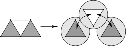
Figure 3. Each simplex is viewed as being contained in an open set on which a tetrad is locally defined. Transition maps mediate between different tetrad patches and hence between different simplex gauges.

In fact we will use these transition maps as the new unknowns, but we will parameterise them through their action on the tetrad and the connection forms. Let the dyad and the connection in the upwards directed triangle be $\{\boldsymbol{\theta}^{0},\boldsymbol{\theta}^{1},\boldsymbol{\omega}\}$, and in the downwards directed face $\{\bar{{\boldsymbol{\theta}}}^{0},\bar{{\boldsymbol{\theta}}}^{1},\bar{\boldsymbol{\omega}}\}$. Furthermore let $[n_{1},n_{2}]$ be the common edge of the two simplices.

In two dimensions a Lorentz transformation is completely determined by a single parameter, its rapidity $\psi$. Hence the action of the transition function has the form

(20) $$\bar{\boldsymbol{\theta}}^{0} =\cosh\psi\boldsymbol{\theta}^{0}+\sinh\psi\boldsymbol{\theta}^{1}, \bar{\boldsymbol{\theta}}^{1} =\cosh\psi\boldsymbol{\theta}^{1}+\sinh\psi\boldsymbol{\theta}^{0}, \bar{\boldsymbol{\omega}} =\boldsymbol{\omega}-\mathbf{d}\psi.$$

On the discrete level the rapidity $\psi$ can be seen as a 0-form, i.e. a map that assigns a number to each node. Yet, in the intersection of two tetrad patches there are only two nodes $n_{1}$ and $n_{2}$, and hence the discretised transition map is determined by two parameters $\psi_{1}=\psi[n_{1}]$ and $\psi_{2}=\psi[n_{2}]$.

Assuming that these parameters are small we may perform a Taylor expansion of (20). The result is that in the leading order $\boldsymbol{\theta}^{0/1}[n_{1},n_{2}]-\bar{\boldsymbol{\theta}}^{0/1}[n_{1},n_{2}]$ depends on the sum $(\psi_{1}+\psi_{2})$, but $\boldsymbol{\omega}[n_{1},n_{2}]-\bar{\boldsymbol{\omega}}[n_{1},n_{2}]$ depends on the difference $(\psi_{1}-\psi_{2})$. Hence we can choose the parameters $\psi_{1}$ and $\psi_{2}$ such that the values of $\bar{{\boldsymbol{\theta}}}^{i}$ and ${\boldsymbol{\theta}}^{i}$ at $[n_{1},n_{2}]$ are the same, while the values of $\bar{\boldsymbol{\omega}}$ and ${\boldsymbol{\omega}}$ differ.

With the two differences of the gauge parameters along the two light-like edges of the upwards directed face we obtain two new unknowns. Effectively, this is the same as forgetting about the value of $\boldsymbol{\omega}$ at these edges. Hence the two additional unknowns are the values of $\bar{\boldsymbol{\omega}}$ at the light-like edges.

It is known from the continuous theory that this regauging should be possible, but it is not known what kind of restrictions are imposed on the gauge parameter by the discretisation. Thus, we assume that this procedure is allowed and check with numerical tests whether this is true.

3.5. Scheme III

The third scheme is based on the system (9),(11). This scheme is a modification of scheme II in the following sense. In section 2 we discussed that (19) can be interpreted as $\boldsymbol{\alpha}=\star\boldsymbol{\beta}$. When evaluated on the light-like edges of upwards directed faces, this formula implies

(21) $$(\boldsymbol{\alpha}-\boldsymbol{\beta})[n_{0},n_{2}]=0=(\boldsymbol{\alpha}+\boldsymbol{\beta})[n_{1},n_{2}].$$

These are equations on the two light-like edges. So, instead of two 2-form equations we have two 1-form equations.

This reinterpretation of (19) does not change the number of equations for upwards directed faces, but it does change it for downwards directed ones. The new 1-form equations are of course already satisfied at the light-like edges, so we loose two equations and we need no regauging, since the number of equations and unknowns are already equal.

In order to test the influence of the gauge choice at the upwards directed faces we make another change. We will not use $\boldsymbol{\omega}[n_{0},n_{2}]=0$, but

(22) $$\boldsymbol{\omega}[n_{0},n_{2}]+\boldsymbol{\omega}[n_{1},n_{2}]=0$$

instead. This is an implicit and non-local definition of the gauge, but it has the advantage that the edges $[n_{0},n_{2}]$ and $[n_{1},n_{2}]$ are treated on a par.

An obvious problem of this scheme is that the discretisation (21) of the Hodge-$\star$ operator can only be applied when two edges of every face are light-like. Clearly this limits its applicability and the question occurs whether a similar discrete Hodge operator exists for space-like and time-like edges. Unfortunately we did not find such a discretisation, but we want to point out what we believe are the first steps to find a more general discrete Hodge operator with similar properties as (21).

For the nodes $x$, $y$ and $z$ we may interpret the edges $e=[x,y]$ and $\bar{e}=[x,z]$, as vectors in the tangent space at $x$. The 2-dimensional Hodge operator is defined through the equation

(23) $$\boldsymbol{\beta}\wedge\star\boldsymbol{\alpha}=g^{-1}(\boldsymbol{\beta},\boldsymbol{\alpha})\boldsymbol{\theta}^{0}\boldsymbol{\theta}^{1}\quad\forall\boldsymbol{\beta}.$$

Applying (23) to the “vectors” $e$ and $\bar{e}$ and identifying the result of applying $\boldsymbol{\alpha}$ and $\star\boldsymbol{\alpha}$ to these vectors with $\boldsymbol{\alpha}[e]$, $\boldsymbol{\alpha}[\bar{e}]$, $\star\boldsymbol{\alpha}[e]$ and $\star\boldsymbol{\alpha}[\bar{e}]$ appropriately leads to

(30) $$\left(\begin{array}[]{c}\star\boldsymbol{\alpha}[e]\\ \star\boldsymbol{\alpha}[\bar{e}]\end{array}\right) =\frac{1}{e^{0}\bar{e}^{1}-e^{1}\bar{e}^{0}}\left(\begin{array}[]{cc}e^{1}\bar{e}^{1}-e^{0}\bar{e}^{0}&e^{0}e^{0}-e^{1}e^{1}\\ \bar{e}^{1}\bar{e}^{1}-\bar{e}^{0}\bar{e}^{0}&e^{0}\bar{e}^{0}-e^{1}\bar{e}^{1}\end{array}\right)\left(\begin{array}[]{c}\boldsymbol{\alpha}[e]\\ \boldsymbol{\alpha}[\bar{e}]\end{array}\right),$$

with $e^{i}=\boldsymbol{\theta}^{i}[e]$, $\bar{e}^{i}=\boldsymbol{\theta}^{i}[\bar{e}]$. This is a possible definition of a discrete Hodge operator that can also be applied to non light-like edges, and when $e$ or $\bar{e}$ is light-like it becomes the discrete Hodge operator (21).

However, we identified the edges with vectors at $x$. In principle there is no reason that e.g. $e$ is a vector at $x$ and not at $y$. But imposing the analogue of (30) at $y$ and $z$ leads to an inconsistent system. Thus the question is how to formulate a discrete geometry in a consistent way. This will be the topic of future investigations.

4. Test scenarios

Having clarified how we apply discrete differential forms in General Relativity, we now describe how we tested the obtained code. Since the spherically symmetric vacuum solutions of the Einstein field equations are all contained within the Kruskal solution [24] for some value of the mass parameter $M$ we know the exact solutions for our problem. The Kruskal metric has in the standard coordinate system the form

(31) $$g=f(R)\left(\mathbf{d}T\otimes\mathbf{d}T-\mathbf{d}X\otimes\mathbf{d}X\right)-R^{2}\left(\mathbf{d}\vartheta\otimes\mathbf{d}\vartheta+\sin^{2}\vartheta\,\mathbf{d}\varphi\otimes\mathbf{d}\varphi\right).$$

There the functions $f(R)$ and $R=R(T,X)$ are defined through

(32) $$f(R) =\frac{32M^{3}}{R}e^{-\frac{R}{2M}}, R(T,X) =2M\left(1+W\left((X^{2}-T^{2})/e\right)\right),$$

where $W$ is the Lambert W-function [25]. To start the time evolution we need initial data which we obtain from one of the analytic solutions. These data must be given as edge- and node values.

4.1. The continuous forms

The best way to do this is to find a description of the geometry, that uses (continuous) differential forms, i.e. maps from the set of all submanifolds to the real numbers. However, such an (abstract) map can hardly be useful for concrete calculations, because without coordinates it is even difficult to describe the position of a point. Therefore we take coordinate representations of the Minkowski and Schwarzschild geometries. For the Schwarzschild geometry it is convenient to use Kruskal coordinates, because then the light-like curves (which are special for the described method) take a very simple form and hence it is easier to compare the results.

To obtain the differential forms, we make a gauge choice, i.e. we choose $\boldsymbol{\theta}^{0}$ and $\boldsymbol{\theta}^{1}$, such that they generate the corresponding metric. In Minkowski space the natural choice is

(33) $$\boldsymbol{\theta}^{0} =\mathbf{d}t, \boldsymbol{\theta}^{1} =\mathbf{d}r, \boldsymbol{\alpha} =\frac{\mathbf{d}r}{r}, \boldsymbol{\beta} =\frac{\mathbf{d}t}{r},$$

$$\boldsymbol{\omega} =0, R^{2} =r^{2}, f_{0} =0, f_{1} =\frac{1}{r},$$

where $r$ and $t$ are the standard space and time coordinate, respectively.

In Kruskal coordinates we use, with the standard space and time coordinates $X$ and $T$, as well as the mass parameter $M$,

(34a) $$\boldsymbol{\theta}^{0} =\sqrt{f(R)}dT, \boldsymbol{\theta}^{1} =\sqrt{f(R)}dX,$$

(34b) $$f_{0} =-\frac{Th(R)}{\sqrt{f(R)}}, f_{1} =\frac{Xh(R)}{\sqrt{f(R)}},$$

(34c) $$\boldsymbol{\alpha} =h(R)(XdX-TdT), \boldsymbol{\beta} =h(R)(XdT-TdX),$$

(34d) $$\boldsymbol{\omega} =g(R)(TdX-XdT), R^{2} =4M^{2}\left(1+W\left((X^{2}-T^{2})/e\right)\right)^{2},$$

where the functions $h$ and $g$ are defined through

(35a) $$h(R) =\frac{8M^{2}}{R^{2}}e^{-\frac{R}{2M}},$$

(35b) $$g(R) =\frac{4M^{2}}{R}\left(\frac{1}{R}+\frac{1}{2M}\right)e^{-\frac{R}{2M}}.$$

4.2. Getting initial values

Next an initial hypersurface has to be chosen. For the test we used curves, whose space-time coordinates $(y^{0},y^{1})$ depend linearly on the curve parameter. These curves will be called “straight”:

(36) $$\left(\begin{array}[]{c}y^{0}\\ y^{1}\end{array}\right)=\left(\begin{array}[]{c}y_{0}^{0}\\ y_{0}^{1}\end{array}\right)+\lambda\left(\begin{array}[]{c}y_{1}^{0}\\ y_{1}^{1}\end{array}\right),$$

for some $\lambda\in[0,1]$ and fixed $y_{0}^{0},y_{0}^{1},y_{1}^{0},y_{1}^{1}$.

We get the initial edges and nodes by subdividing this curve into pieces of equal ‘coordinate length’. That is we start at a hypersurface of the form (36) with boundary at $\lambda=0$ and $\lambda=1$ and subdivide it into $n$ pieces. The pieces are again straight, and $\lambda$ takes values in the intervals $[(i-1)/n,i/n],\;i=1,\ldots,n$. On the edges we can integrate the continuous 1-forms known from the analytic solution, and the results are the initial values for the corresponding discrete 1-forms.

To get initial values for the 0-forms, we evaluate the corresponding continuous functions at the boundary points $\lambda=i/n,\;i=0,\ldots,n$ of the sub-intervals. These values are invariant under coordinate transformations so that we do not start with coordinate dependent values in the beginning.

4.3. Examination of the results

In order to compare the numerical results with the analytical solution we need to determine the location in space-time of the nodes and edges used in the algorithm. This can be a difficult task because in principle one needs to solve the geodesic equations to obtain the light rays used to define the nodes in the next time-slice. However, here this is very much simplified since in Kruskal coordinates as well as in Minkowski coordinates the radial light rays move on straight lines.

When comparing the results we need to worry about the gauge. I.e. when we use different gauges for the discrete approximation and for the analytic solution, we cannot expect to get the same results. However, if the method is feasible, we can expect that gauge invariant discrete variables are good approximations of the continuous ones. Gauge independent values are for instance the lengths $l=\sqrt{|(\boldsymbol{\theta}^{0})^{2}-(\boldsymbol{\theta}^{1})^{2}|}$ of the space-like edges, the values of the 1-form $\boldsymbol{\alpha}$ on these edges and the values of the function $R^{-2}$ at the nodes.

Another way to evaluate a numerical method is a self-convergence test. There one compares solutions obtained on coarse meshes with a solution that is calculated on a fine mesh. It is clear that a method that converges to the analytical solution when the mesh is refined is self-convergent, too.

5. Results

For the number of initial edges we have always chosen a power of two ($n=2^{i},\;i=1,2,3,\ldots$), and calculated half of the maximal number of time-steps: for $n$ initial edges, we calculate $n/2$ time-steps. The last time-step then contains $n/2$ downwards directed simplices. Each of these simplices contains one non light-like edge and each of these edges contains two nodes. Altogether these are $n/2$ edges and $(n/2+1)$ nodes, since nodes of adjacent edges coincide.

It turns out that the computational costs of the three schemes are quite comparable. In scheme I the solution in a mesh with approximately 200.000 faces is obtained in one minute on a 700MHz PC. In schemes II and III it takes about 40% and 10% longer respectively. This could be expected, because in scheme I one has to solve systems of six and three equations for the upwards and downwards directed triangles respectively. In schemes II and III the sizes of these systems are seven and seven, respectively seven and five. Thus, in scheme I the number of equations is much smaller. Clearly, since there is a system of equations on each individual face, the time that is needed to find the solution depends linearly on the number of faces, and hence quadratically on the number of initial edges.

In the left diagrams of Figs. 4, 5 and 6 we show the maxima over the $n/2$ edges of the relative errors in the values of the 1-form $\boldsymbol{\alpha}$ for schemes II and III as well as the maxima over the $(n/2+1)$ nodes of the relative errors in the values of $R^{-2}$ for scheme I. In the right diagrams of Figs. 4, 5 and 6 the maxima over the $n/2$ edges of the relative error of the invariant lengths $l$ are plotted.

5.1. Minkowski space-time

Figure 4. Maximal relative errors in Minkowski space-time. Left: values of $R^{-2}$ at the nodes (scheme I) and values of $\boldsymbol{\alpha}$ at the space-like edges (schemes II,III). Right: invariant lengths of space-like edges.

For the initial hypersurface we have chosen the set $\{(t,r)=(0,1+\lambda):\lambda\in[0,1]\}$, with the standard time and space coordinates $t$ and $r$, respectively. We compare the results with the analytic solution at the hypersurface $\{(t,r)=(0.25,1.25+\lambda/2):\lambda\in[0,1]\}$.

We see from figure 4, that the relative error converges for all three schemes quadratically to zero when the typical size of simplices in the mesh is decreased. The error of the lengths is about 100 times bigger for scheme I, but it remains small even for the coarsest mesh.

5.2. Kruskal geometry

In Kruskal geometry we test the code for one space-like and one time-like initial hypersurface. Since in Kruskal coordinates the horizon is a regular null-hypersurface we can test how the code behaves near the event horizon. So, we take the space-like curve to cross the horizon.

5.2.1. Space-like initial data

In $(T,X)$-coordinates we choose the initial hypersurface $\{T=\lambda/2,X=-1+2\lambda,\lambda\in[0,1]\}$, and compare the results at the hypersurface $\{T=5/8+\lambda/4,X=-3/8+\lambda,\lambda\in[0,1]\}$.

Figure 5. Maximal relative errors in Kruskal space-time (space-like initial data). Left: values of $R^{-2}$ at the nodes (scheme I) and values of $\boldsymbol{\alpha}$ at the space-like edges (schemes II,III). Right: invariant lengths of space-like edges.

Fig. 5 shows that the schemes I and III provide small errors and the relative error converges quadratically to zero when the size of the simplices is decreased. The errors in scheme II on the other hand are very big, and even become bigger when the mesh is refined. Clearly this points to a problem in scheme II that we discuss later.

5.2.2. Time-like initial data

In $(T,X)$-coordinates we choose the initial hypersurface $\{T=\lambda,X=3,\lambda\in[0,1]\}$. The comparison of the results is done at the hypersurface $\{T=0.25+\lambda/2,X=3.25,\lambda\in[0,1]\}$.

Figure 6. Maximal relative errors in Kruskal space-time (time-like initial data). Left: values of $R^{-2}$ at the nodes (scheme I) and values of $\boldsymbol{\alpha}$ at the space-like edges (schemes II,III). Right: invariant lengths of space-like edges.

Again, as can be seen in Fig. 6, schemes I and III provide very small errors that converge quadratically to zero when the simplex size is reduced. With 1% for $\boldsymbol{\alpha}$ and 10% for the lengths the errors of scheme II are in this case also quite small. However, the relative errors do not become smaller for finer meshes.

Since in fig. 6 one sees that the errors of the results in fine meshes are nearly the same as the errors in coarse meshes, we also performed a self-convergence test, where the number of initial edges in the finest mesh was 2048. The result is that scheme II converges linearly to a solution that differs from the analytical one.

6. Discussion

From the results presented in the last section we conclude that the schemes I and III provide very good results. Especially scheme III converges quadratically to the analytical solution in every simulation we performed. Also in scheme I most of the simulations led to quadratically convergent results. There are only a few regions in Kruskal space-time where the errors of this scheme become quite large. This is the the case for $R\approx 3M$. The reason for this is, that there two solutions of the discrete equations are close to each other. The root finding algorithm then sometimes chooses the wrong one. However, this should be solvable with an optimised choice of starting values for the Newton iteration, but we did not find a practical way to obtain such starting values.

The errors obtained with scheme II are on the other hand quite large. This scheme is in some situations not convergent and its behaviour strongly depends on the initial data. We conclude that it is not feasible for numerical calculations and thus seems to be ill-posed. Now, the question is what the reasons for these problems are.

The difference between the schemes II and III was the direct implementation of the Hodge operator in scheme III while scheme II made use of the equations (19), which have been added to the system in order to encode the duality between the forms $\boldsymbol{\alpha}$ and $\boldsymbol{\beta}$. It turns out, that far from the horizon in the exterior the values of $\boldsymbol{\alpha}$ on the space-like edges are much smaller than the values of $\boldsymbol{\beta}$, while far from the horizon in the interior it is the other way round. Near the horizon the two 1-forms interchange their role in this sense, and are hence of comparable size.

Near the horizon the solution of (19) largely differs from $\boldsymbol{\alpha}=\pm\boldsymbol{\beta}$. This property appeared in all simulation where the initial hypersurface crossed the horizon, especially it seems to be independent of the location of the nodes in the initial hypersurface. The origin of this behaviour seems to be the ill-conditioning of the linear system corresponding to (19). Thus (19) is a bad implementation of the Hodge operator in that region.

Clearly the Hodge operator (21) leads to a convergent scheme. However, (21) was inspired by the dual mesh of electrodynamics. In a $(1+1)$-dimensional Lorentz geometry it is convenient to define the dual of a light-like edge to be the edge itself.

Yet, we wanted to avoid the construction of a dual mesh. The first reason for this decision is that without a dual mesh the discrete system decouples into small systems for every face. The second reason is that the dual of an initial edge does not lie in the initial hypersurface and hence we do not know how to specify initial values for it. The third reason is that the dual cells are in general not simplices anymore, which causes problems in defining a natural discrete exterior product without ambiguities.

The discrete Hodge operator (19) also made it necessary to use the regauging described in section 3.4. Although we cannot make definite statments about this procedure yet, it seems that it is also a source of errors in scheme II. These problems probably arise because the notion of a gauge transformation for the discrete equations has not been clarified completely so far. This is planned to be the topic of future investiagtions.

7. Conclusion

In this article we presented first results of the application of discrete differential forms in General Relativity. It was shown, that the method is quite promising. Several schemes were found whose results are close to the analytic solution and the errors of which converge quadratically to zero.

We discussed that one has to be careful with the definition of discrete Hodge operators and that the notion of discrete gauge transformations is not completely understood. Making a wrong decision in these fields can lead to results with big errors.

Now one has to get a better understanding of gauge transformations for the discrete equations, a more general definition of the Hodge operator is necessary to be able to include matter fields and the method must be applied in space-times with smaller symmetry groups, in order to get physically more relevant solutions.

Appendix A Derivation of the reduced system

A.1. Spherical symmetry

In this appendix we will derive the reduced exterior system (7). So we assume the existence of an isometric action of the rotation group $G=SO(3)$ on the space-time manifold i.e., for each element $a\in G$ there is an isometry $\phi_{a}$ of $({\mathcal{M}},g)$. We assume that the orbits of this action are 2-dimensional submanifolds except for the fixed points, which form a 1-dimensional submanifold, called the origin $\mathcal{O}$. Clearly, the 2-dimensional orbits are round spheres, they carry an induced metric which is a constant multiple of the unit-sphere metric.

Given a point $p\in{\mathcal{M}}\setminus\mathcal{O}$ and the orbit $S_{p}$ through $p$ we can split $T_{p}\mathcal{M}$ into the 2-dimensional tangent space $\mathbb{H}_{p}$ of $S_{p}$ at $p$, which we call the horizontal space and its orthogonal complement $\mathbb{V}_{p}$, the vertical space. The isometric action maps vertical spaces into vertical ones and horizontal spaces into horizontal ones. Fix a point $p$ then the isotropy group of $p$ is isomorphic to $SO(2)$ and the symmetry action defines a representation of $SO(2)$ on $\mathbb{H}_{p}$. This is isomorphic to the defining representation. On the other hand, the isotropy group of $p$ acts trivially on $\mathbb{V}_{p}$. This follows from the fact that such an action defines a homomorphism from $SO(2)$ to $SO(1,1)$. Due to the different topologies of these groups this must be trivial.

We will be concerned with invariant objects, i.e., objects which are mapped onto themselves by this symmetry action. Consider an invariant function $f$. It satisfies $\phi_{a}^{*}f=f\circ\phi_{a}=f$ for every rotation $a\in G$. This implies that $f$ must be constant on each orbit because for any two points on a given orbit there is a rotation which maps one to the other.

An invariant vectorfield $\mathbf{V}$ coincides with each push-forward, i.e., $\phi_{a*}\mathbf{V}=\mathbf{V}$. Suppose $\mathbf{V}$ is horizontal then it follows from the free action of the isotropy groups on the horizontal spaces that $\mathbf{V}$ must indeed vanish because at each point $p$ it must coincide with all its images under elements of the isotropy group. Thus, an invariant vectorfield cannot have horizontal components so it is always vertical. It follows from this that the covariant derivative of an invariant vectorfield along an invariant vectorfield is again invariant, hence vertical. Also the commutator of two invariant vectorfields is vertical. This implies that the subbundle of the tangent bundle consisting of vertical vectors forms an integrable distribution: any vertical vectorfield $\mathbf{U}$ can be written as a linear combination of invariant vectorfields $\mathbf{X}_{1}$ and $\mathbf{X}_{2}$

(37) $$\mathbf{U}=U^{1}\mathbf{X}_{1}+U^{2}\mathbf{X}_{2}$$

so that the commutator of two such vectorfields is

(38) $$\left[\mathbf{U},\mathbf{V}\right]=\mathbf{U}(V^{i})\mathbf{X}_{i}-\mathbf{V}(U^{i})\mathbf{X}_{i}+U^{i}V^{k}\left[\mathbf{X}_{i},\mathbf{X}_{k}\right],$$

hence it is vertical. The maximal integral manifolds will be called vertical surfaces. This discussion shows that the space-time has the topology ${\mathcal{M}}={\mathcal{M}}_{1}\times S^{2}$ where ${\mathcal{M}}_{1}$ is a two-dimensional manifold. We define the two canonical projections

(39) $$\pi:{\mathcal{M}}\to{\mathcal{M}}_{1},\qquad\rho:{\mathcal{M}}\to S^{2}$$

mapping on the first, resp. second factor.

We can set up adapted local coordinates as follows. Fix a point $p$ and assign to it the coordinates $(x^{0},x^{1},x^{2},x^{3})$ where $(x^{0},x^{1})$ are local coordinates near $\pi(p)\in{\mathcal{M}}_{1}$ and $(x^{2},x^{3})$ are local coordinates near $\rho(p)\in S^{2}$. In these coordinates the projections are $\pi(x^{0},x^{1},x^{2},x^{3})=(x^{0},x^{1})$ and $\rho(x^{0},x^{1},x^{2},x^{3})=(x^{2},x^{3})$.

We recall the following facts. The projections $\pi$ and $\rho$ induce isomorphisms between $\mathbb{V}_{p}$ and $T_{\pi(p)}{\mathcal{M}}_{1}$ resp. $\mathbb{H}_{p}$ and $T_{\rho(p)}S^{2}$. The group action happens only on the second factor, i.e., $\pi\circ\phi_{a}=\pi$. This implies that $p$-forms on ${\mathcal{M}}$ which are pull-backs from ${\mathcal{M}}_{1}$ are invariant and annihilate horizontal vectors. Conversely, a $p$-form on ${\mathcal{M}}$ which is invariant and annihilates horizontal vectors is the pull-back of a form on ${\mathcal{M}}_{1}$. This is true for any multilinear map. Furthermore, invariant vectorfields (which are necessarily vertical) project down to a well-defined vectorfield on ${\mathcal{M}}_{1}$ and each vectorfield on ${\mathcal{M}}_{1}$ corresponds to an invariant vectorfield on ${\mathcal{M}}$.

The metric on ${\mathcal{M}}$ can be written in the form

(40) $$g=g_{1}+g_{2}$$

where $g_{1}$ ($g_{2}$) is non-zero only for vertical (horizontal) vectors. This shows that the topological decomposition is also an orthogonal decomposition. Furthermore, for any infinitesimal isometry $\xi$ we have

(41) $$0={\mathcal{L}}_{\xi}g={\mathcal{L}}_{\xi}g_{1}+{\mathcal{L}}_{\xi}g_{2}$$

and the orthogonality properties imply that the two terms on the right have to vanish separately,

(42) $${\mathcal{L}}_{\xi}g_{1}=0={\mathcal{L}}_{\xi}g_{2}.$$

Now, the facts that ${\mathcal{L}}_{\xi}g_{1}=0$ and that $g_{1}(X,\cdot)$ vanishes for any horizontal vector $X$ imply that $g_{1}$ is the pull-back of a metric $h$ on ${\mathcal{M}}_{1}$.

The metric $g_{2}$ is conformal to the metric $\delta$ on the unit sphere $S^{2}$ where the conformal factor may depend on the coordinates $(x^{0},x^{1})$. Thus, we can write the space-time metric in the form of a warped product

(43) $$g=\pi^{*}h+R^{2}\rho^{*}\delta\qquad\text{where }R^{2}:{\mathcal{M}}_{1}\to{\mathbb{R}}$$

We can now set up an adapted tetrad $(\boldsymbol{\theta}^{i})_{i=0:3}$. To this end we choose a frame $(\boldsymbol{\vartheta}^{0},\boldsymbol{\vartheta}^{1})$ on $({\mathcal{M}}_{1},h)$ and a frame $(\boldsymbol{\vartheta}^{2},\boldsymbol{\vartheta}^{3})$ on $(S^{2},\delta)$ and set

(44) $$(\boldsymbol{\theta}^{0},\boldsymbol{\theta}^{1},\boldsymbol{\theta}^{2},\boldsymbol{\theta}^{3})=(\pi^{*}\boldsymbol{\vartheta}^{0},\pi^{*}\boldsymbol{\vartheta}^{1},R\,\rho^{*}\boldsymbol{\vartheta}^{2},R\,\rho^{*}\boldsymbol{\vartheta}^{3}).$$

Using this tetrad in the first structure equation one finds after some calculation that the connection forms are

(45) $$\boldsymbol{\omega}^{0}{}_{1} =\pi^{*}\boldsymbol{\omega},\quad \boldsymbol{\omega}^{2}{}_{0} =f_{0}\boldsymbol{\theta}^{2},\quad \boldsymbol{\omega}^{3}{}_{0} =f_{0}\boldsymbol{\theta}^{3},$$

$$\boldsymbol{\omega}^{2}{}_{3} =\rho^{*}\boldsymbol{\varpi}, \boldsymbol{\omega}^{2}{}_{1} =f_{1}\boldsymbol{\theta}^{2}, \boldsymbol{\omega}^{3}{}_{1} =f_{1}\boldsymbol{\theta}^{3}.$$

Here, $\boldsymbol{\omega}$ resp. $\boldsymbol{\varpi}$ are the connection forms of the metrics on ${\mathcal{M}}_{1}$ resp. $S^{2}$ and

(46) $$\boldsymbol{\alpha}\equiv f_{0}\boldsymbol{\theta}^{0}+f_{1}\boldsymbol{\theta}^{1}=\mathbf{d}R/R$$

is an invariant 1-form on ${\mathcal{M}}_{1}$.

Appendix B Reduction to 1+1 dimensions

Our goal is to express the field equations (5) as equations on ${\mathcal{M}}_{1}$. The easiest way to achieve this goal is to compute the Nester-Witten and Sparling forms from the connection forms (45). This yields the following result

(47a) $$L_{0} =2f_{1}\boldsymbol{\theta}^{2}\boldsymbol{\theta}^{3}-\boldsymbol{\omega}^{2}{}_{3}\boldsymbol{\theta}^{1}, L_{2} =-f_{1}\boldsymbol{\theta}^{0}\boldsymbol{\theta}^{3}-f_{0}\boldsymbol{\theta}^{1}\boldsymbol{\theta}^{3}-\boldsymbol{\omega}^{0}{}_{1}\boldsymbol{\theta}^{3},$$

(47b) $$L_{1} =2f_{0}\boldsymbol{\theta}^{2}\boldsymbol{\theta}^{3}+\boldsymbol{\omega}^{2}{}_{3}\boldsymbol{\theta}^{0}, L_{3} =f_{1}\boldsymbol{\theta}^{0}\boldsymbol{\theta}^{2}+f_{0}\boldsymbol{\theta}^{1}\boldsymbol{\theta}^{2}+\boldsymbol{\omega}^{0}{}_{1}\boldsymbol{\theta}^{2}$$

for the Nester-Witten form, while the Sparling 3-form is given by

(48a) $$S_{0} =2f_{0}f_{1}\boldsymbol{\theta}^{0}\boldsymbol{\theta}^{2}\boldsymbol{\theta}^{3}+(f_{0}^{2}+f_{1}^{2})\boldsymbol{\theta}^{1}\boldsymbol{\theta}^{2}\boldsymbol{\theta}^{3}+2f_{0}\boldsymbol{\omega}^{0}{}_{1}\boldsymbol{\theta}^{2}\boldsymbol{\theta}^{3}-\boldsymbol{\omega}^{2}{}_{3}\boldsymbol{\omega}^{0}{}_{1}\boldsymbol{\theta}^{0},$$

(48b) $$S_{1} =2f_{0}f_{1}\boldsymbol{\theta}^{1}\boldsymbol{\theta}^{2}\boldsymbol{\theta}^{3}+(f_{0}^{2}+f_{1}^{2})\boldsymbol{\theta}^{0}\boldsymbol{\theta}^{2}\boldsymbol{\theta}^{3}+2f_{1}\boldsymbol{\omega}^{0}{}_{1}\boldsymbol{\theta}^{2}\boldsymbol{\theta}^{3}+\boldsymbol{\omega}^{2}{}_{3}\boldsymbol{\omega}^{0}{}_{1}\boldsymbol{\theta}^{1},$$

(48c) $$S_{2} =f_{0}\boldsymbol{\omega}^{0}{}_{1}\boldsymbol{\theta}^{0}\boldsymbol{\theta}^{3}-f_{0}\boldsymbol{\omega}^{2}{}_{3}\boldsymbol{\theta}^{1}\boldsymbol{\theta}^{2}+f_{1}\boldsymbol{\omega}^{0}{}_{1}\boldsymbol{\theta}^{1}\boldsymbol{\theta}^{3}-f_{1}\boldsymbol{\omega}^{2}{}_{3}\boldsymbol{\theta}^{0}\boldsymbol{\theta}^{2}+\boldsymbol{\omega}^{0}{}_{1}\boldsymbol{\omega}^{2}{}_{3}\boldsymbol{\theta}^{2},$$

(48d) $$S_{3} =-f_{0}\boldsymbol{\omega}^{0}{}_{1}\boldsymbol{\theta}^{0}\boldsymbol{\theta}^{2}-f_{0}\boldsymbol{\omega}^{2}{}_{3}\boldsymbol{\theta}^{1}\boldsymbol{\theta}^{3}-f_{1}\boldsymbol{\omega}^{0}{}_{1}\boldsymbol{\theta}^{1}\boldsymbol{\theta}^{2}-f_{1}\boldsymbol{\omega}^{2}{}_{3}\boldsymbol{\theta}^{0}\boldsymbol{\theta}^{3}+\boldsymbol{\omega}^{0}{}_{1}\boldsymbol{\omega}^{2}{}_{3}\boldsymbol{\theta}^{3}.$$

Let us now compute the exterior derivative of $L_{0}$. We obtain

(49) $$\mathbf{d}L_{0}=2\mathbf{d}f_{1}\boldsymbol{\theta}^{2}\boldsymbol{\theta}^{3}+2f_{1}\mathbf{d}(\boldsymbol{\theta}^{2}\boldsymbol{\theta}^{3})-\mathbf{d}\boldsymbol{\omega}^{2}{}_{3}\boldsymbol{\theta}^{1}+\boldsymbol{\omega}^{2}{}_{3}\mathbf{d}\boldsymbol{\theta}^{1}.$$

Since $\boldsymbol{\theta}^{2}\boldsymbol{\theta}^{3}=R^{2}\rho^{*}(\boldsymbol{\vartheta}^{2}\boldsymbol{\vartheta}^{3})$ we find

(50) $$\mathbf{d}(\boldsymbol{\theta}^{2}\boldsymbol{\theta}^{3})=\frac{\mathbf{d}R^{2}}{R^{2}}\boldsymbol{\theta}^{2}\boldsymbol{\theta}^{3}$$

and for $\mathbf{d}\boldsymbol{\omega}^{2}{}_{3}$ we obtain

(51) $$\mathbf{d}\boldsymbol{\omega}^{2}{}_{3}=\rho^{*}\mathbf{d}\boldsymbol{\varpi}=\rho^{*}\boldsymbol{\Omega}$$

where $\boldsymbol{\Omega}$ is the curvature 2-form of the unit sphere which is given by $\boldsymbol{\Omega}=\boldsymbol{\vartheta}^{2}\boldsymbol{\vartheta}^{3}$. Hence,

(52) $$\mathbf{d}\boldsymbol{\omega}^{2}{}_{3}=\rho^{*}(\boldsymbol{\vartheta}^{2}\boldsymbol{\vartheta}^{3})=\frac{1}{R^{2}}\boldsymbol{\theta}^{2}\boldsymbol{\theta}^{3}.$$

Furthermore, making use of the structure of the connection forms we have

(53) $$\mathbf{d}\boldsymbol{\theta}^{1}=-\boldsymbol{\omega}^{1}{}_{0}\boldsymbol{\theta}^{0}-\boldsymbol{\omega}^{1}{}_{2}\boldsymbol{\theta}^{2}-\boldsymbol{\omega}^{1}{}_{3}\boldsymbol{\theta}^{3}=-\boldsymbol{\omega}^{1}{}_{0}\boldsymbol{\theta}^{0}.$$

This shows that with $\boldsymbol{\theta}^{1}$ also $\mathbf{d}\boldsymbol{\theta}^{1}$ is invariant (this also follows from the fact that $\boldsymbol{\theta}^{1}=\pi^{*}\boldsymbol{\vartheta}^{1}$ so that $\mathbf{d}\boldsymbol{\theta}^{1}=\pi^{*}\mathbf{d}\boldsymbol{\vartheta}^{1}$). Taken together, we have

(54) $$\mathbf{d}L_{0} =\left(2\mathbf{d}f_{1}+2f_{1}\frac{\mathbf{d}R^{2}}{R^{2}}-\frac{1}{R^{2}}\boldsymbol{\theta}^{1}\right)\boldsymbol{\theta}^{2}\boldsymbol{\theta}^{3}+\boldsymbol{\omega}^{2}{}_{3}\mathbf{d}\boldsymbol{\theta}^{1}$$

$$=\left(2f_{0}f_{1}\boldsymbol{\theta}^{0}+(f_{0}^{2}+f_{1}^{2})\boldsymbol{\theta}^{1}+2f_{0}\boldsymbol{\omega}^{0}{}_{1}\right)\boldsymbol{\theta}^{2}\boldsymbol{\theta}^{3}-\boldsymbol{\omega}^{2}{}_{3}\boldsymbol{\omega}^{0}{}_{1}\boldsymbol{\theta}^{0}.$$

Using (54) and (48a) we write the equation $\mathbf{d}L_{0}=S_{0}$ (which is (5b) for $i=0$) in the form

$$\left(2\mathbf{d}f_{1}+2f_{1}\frac{\mathbf{d}R^{2}}{R^{2}}-\frac{1}{R^{2}}\boldsymbol{\theta}^{1}-2f_{0}f_{1}\boldsymbol{\theta}^{0}-(f_{0}^{2}+f_{1}^{2})\boldsymbol{\theta}^{1}-2f_{0}\boldsymbol{\omega}^{0}{}_{1}\right)\boldsymbol{\theta}^{2}\boldsymbol{\theta}^{3}=0$$

and contract with two horizontal vectors. Then we find the equation

(55) $$2\mathbf{d}f_{1}+2f_{1}\frac{\mathbf{d}R^{2}}{R^{2}}-\frac{1}{R^{2}}\boldsymbol{\theta}^{1}-2f_{0}f_{1}\boldsymbol{\theta}^{0}-(f_{0}^{2}+f_{1}^{2})\boldsymbol{\theta}^{1}-2f_{0}\boldsymbol{\omega}^{0}{}_{1}=0.$$

Conversely, if (55) holds then the field equation $\mathbf{d}L_{0}=S_{0}$ is satisfied. In a similar way we can treat the equation $\mathbf{d}L_{1}=S_{1}$, i.e. (5b) for $i=1$. We obtain

(56) $$2\mathbf{d}f_{0}+2f_{0}\frac{\mathbf{d}R^{2}}{R^{2}}+\frac{1}{R^{2}}\boldsymbol{\theta}^{0}-2f_{0}f_{1}\boldsymbol{\theta}^{1}-(f_{0}^{2}+f_{1}^{2})\boldsymbol{\theta}^{0}-2f_{1}\boldsymbol{\omega}^{0}{}_{1}=0.$$

For $i=2,3$ equation (5b) has to be treated differently. Let us consider the case $i=2$. We first define the invariant 1-form

(57) $$\boldsymbol{\beta}=f_{0}\boldsymbol{\theta}^{1}+f_{1}\boldsymbol{\theta}^{0}$$

and then we derive from (47a)

(58) $$\mathbf{d}L_{2}=-\mathbf{d}(\boldsymbol{\beta}+\boldsymbol{\omega}^{0}{}_{1})\boldsymbol{\theta}^{3}+(\boldsymbol{\beta}+\boldsymbol{\omega}^{0}{}_{1})\mathbf{d}\boldsymbol{\theta}^{3}=-\boldsymbol{\alpha}\boldsymbol{\omega}^{0}{}_{1}\boldsymbol{\theta}^{3}-(\boldsymbol{\beta}+\boldsymbol{\omega}^{0}{}_{1})\boldsymbol{\omega}^{3}{}_{2}\boldsymbol{\theta}^{2}.$$

Using the fact that

(59) $$\mathbf{d}\boldsymbol{\theta}^{3}=-\boldsymbol{\omega}^{3}{}_{0}\boldsymbol{\theta}^{0}-\boldsymbol{\omega}^{3}{}_{1}\boldsymbol{\theta}^{1}-\boldsymbol{\omega}^{3}{}_{2}\boldsymbol{\theta}^{2}=-\boldsymbol{\omega}^{3}{}_{2}\boldsymbol{\theta}^{2}+\boldsymbol{\alpha}\boldsymbol{\theta}^{3}$$

we can write the equation $\mathbf{d}L_{2}=S_{2}$ as

$$\left(\mathbf{d}\boldsymbol{\beta}+\mathbf{d}\boldsymbol{\omega}^{0}{}_{1}+\boldsymbol{\alpha}\boldsymbol{\beta}\right)\boldsymbol{\theta}^{3}=0.$$

Contraction with one horizontal vector shows that this equation implies

(60) $$\mathbf{d}\boldsymbol{\beta}+\mathbf{d}\boldsymbol{\omega}^{0}{}_{1}+\boldsymbol{\alpha}\boldsymbol{\beta}=0$$

and, conversely, if (60) is satisfied then also $\mathbf{d}L_{2}=S_{2}$ holds. The equation $\mathbf{d}L_{3}=S_{3}$ does not contribute anything new.

Now we can collect the equations. The contents of the first structure equation is the specific form of the connection forms, the first structure equation on $S^{2}$ and the first structure equation on ${\mathcal{M}}_{1}$. Since all the relevant quantities are invariant they are pull-backs from ${\mathcal{M}}_{1}$. So the equations really live on ${\mathcal{M}}_{1}$. However, in order not to complicate the notation we will continue to write them as equations on ${\mathcal{M}}$, keeping in mind that everything has to be regarded as a pull-back from the 2-dimensional manifold ${\mathcal{M}}_{1}$. Then we have

(61) $$\mathbf{d}\boldsymbol{\theta}^{0}+\boldsymbol{\omega}^{0}{}_{1}\boldsymbol{\theta}^{1} =0$$

$$\mathbf{d}\boldsymbol{\theta}^{1}+\boldsymbol{\omega}^{1}{}_{0}\boldsymbol{\theta}^{0} =0.$$

Furthermore, we have the relationship between the 1-form $\boldsymbol{\alpha}$ and the differential of $R^{2}$

(62) $$\mathbf{d}R^{2}=2\boldsymbol{\alpha}R^{2}.$$

That means the integral of $\boldsymbol{\alpha}$ along a curve is the same as the difference of the values of $(\log R)$ at the boundary of that curve. Hence $\boldsymbol{\alpha}$ is related the velocity with that the area of the spheres changes.

Then the field equations written in terms of $f_{0}$, $f_{1}$ and $\boldsymbol{\beta}=f_{0}\boldsymbol{\theta}^{1}+f_{1}\boldsymbol{\theta}^{0}$ are

(63) $$\mathbf{d}f_{0}-\boldsymbol{\omega}f_{1}+f_{0}\boldsymbol{\alpha}+\frac{1}{2}\left(f_{0}^{2}-f_{1}^{2}+\frac{1}{R^{2}}\right)\boldsymbol{\theta}^{0} =0,$$

(64) $$\mathbf{d}f_{1}-\boldsymbol{\omega}f_{0}+f_{1}\boldsymbol{\alpha}-\frac{1}{2}\left(f_{0}^{2}-f_{1}^{2}+\frac{1}{R^{2}}\right)\boldsymbol{\theta}^{1} =0,$$

(65) $$\mathbf{d}\boldsymbol{\beta}+\mathbf{d}\boldsymbol{\omega}+\boldsymbol{\alpha}\boldsymbol{\beta} =0.$$

Note, that contracting the first of these equations with $\boldsymbol{\theta}^{0}$ and the second with $\boldsymbol{\theta}^{1}$ yields the integrability condition $\mathbf{d}\boldsymbol{\alpha}=0$. On the other hand, using these two equations to compute the differential of $\boldsymbol{\beta}$ we find

(66) $$\mathbf{d}\boldsymbol{\beta}=-2\boldsymbol{\alpha}\boldsymbol{\beta}-\frac{1}{R^{2}}\boldsymbol{\theta}^{0}\boldsymbol{\theta}^{1}$$

and, therefore,

(67) $$\mathbf{d}\boldsymbol{\omega}=\boldsymbol{\alpha}\boldsymbol{\beta}+\frac{1}{R^{2}}\boldsymbol{\theta}^{0}\boldsymbol{\theta}^{1}.$$

Note, that $\boldsymbol{\alpha}$ and $\boldsymbol{\beta}$ are not independent. They contain the same information. In fact, we have $\boldsymbol{\beta}=\star\boldsymbol{\alpha}$. This relationship can be expressed in the present case also as two 2-form equations

(68) $$\boldsymbol{\alpha}\boldsymbol{\theta}^{1}+\boldsymbol{\beta}\boldsymbol{\theta}^{0}=0,\qquad\boldsymbol{\alpha}\boldsymbol{\theta}^{0}+\boldsymbol{\beta}\boldsymbol{\theta}^{1}=0.$$

This concludes the derivation of the reduced equations.

References

- [1] Regge T, 1961 General Relativity without coordinates. Nouvo Cimento 19 558–571.
- [2] Gentle A P, 2002 Regge calculus: a unique tool for numerical relativity. Gen. Rel. Grav. 34 1701–1718.
- [3] Thornburg, J., 2004 Black-hole excision with multiple grid patches. Class. Quant. Grav. 21 3665–3691
- [4] Scheel, M. A. et al., 2006 Solving Einstein’s Equations With Dual Coordinate Frames. gr-qc/0607056
- [5] Schnetter, E. et al., 2006 A multi-block infrastructure for three-dimensional time-dependent numerical relativity Class. Quant. Grav. 23 S553 – S578
- [6] Frauendiener J, 2006 Discrete differential forms in General Relativity. Class. Quant. Grav. 23 S369–S385.
- [7] Bossavit A, 1998–2000 Discretization of electromagnetic problems. Tech. rep., Interdyscyplinary Centre For Mathematical And Computational Modelling, Warsaw. Http://www.icm.edu.pl/edukacja/mat/DEP.php.
- [8] Bossavit A, 1988 Mixed finite elements and the complex of Whitney forms. In The Mathematics of Finite Elements and Applications VI, ed. J Whiteman (London: Academic Press). pp. 137–144.
- [9] Nédélec J C, 1980 Mixed finite elements in . Numer. Math. 35 315–341.
- [10] Raviart P A and Thomas J M, 1977 A mixed finite element method for 2nd order elliptic problems. In Mathematical aspects of the finite element method, eds. I Galligani and E Magenes (Berlin and New York: Springer-Verlag), vol. 606 of Lecture Notes in Mathematics.
- [11] Hiptmair R, 2002 Finite elements in computational electromagnetism. Acta Numerica 11 237–339.
- [12] Bossavit A, 1998 Computational Electromagnetism (Boston: Academic Press).
- [13] Sopuerta, C. F. and Laguna, P., 2006 Finite element computation of the gravitational radiation emitted by a pointlike object orbiting a nonrotating black hole Phys. Rev. D 73 044028
- [14] Cartan É, 2001 Riemannian Geometry In An Orthogonal Frame (Singapore: World Scientific). Lectures delivered by E. Cartan at the Sorbonne 1926-27.
- [15] Sparling G, 2001 Twistors, spinors and the Einstein equations. In Further advances in twistor theory III: Curved twistor spaces, eds. L J Mason, L P Hughston, P Z Kobak and K Pulverer (Boca Raton: Chapman and Hall). pp. 179–187.
- [16] Landau, L D and Lifschitz, E F, 1975 The Classical Theory of Fields (Oxford: Pergamon Press)
- [17] Frankel T, 1997 The geometry of Physics – An introduction (Cambridge: Cambridge University press).
- [18] Whitney H, 1957 Geometric Integration Theory (Princeton: Princeton University Press).
- [19] Gradinaru V and Hiptmair R, 1999 Whitney elements on pyramids. ETNA 8 154–168.
- [20] Munkres J R, 1993 Simplicial complexes and simplicial maps. In Elements of Algebraic Topology (Perseus Press), chap. 1.2. pp. 7–14.
- [21] Powell M J D, 1970 A hybrid method for nonlinear equations. In Numerical Methods for Nonlinear Algebraic Equations, ed. P Rabinowitz (Gordon and Breach).
- [22] Galassi M et al., 2005 GNU Scientific Library Reference Manual. http://www.gnu.org/software/gsl/manual/gsl-ref_toc.html.
- [23] Penrose, R. and Rindler, W., 1986 Spinors and space–time : Spinor and twistor methods in space-time geometry (Cambridge: Cambridge University Press)
- [24] Weinberg, S., 1972 Gravitation and Cosmology : Principles and Applications of the General Theory of Relativity (New York: Wiley).
- [25] Corless R M et al., 1996 On the Lambert W-function. Adv. Comput. Math. 5 329–359.