$\Lambda$XCDM: a cosmon model solution to the cosmological coincidence problem?

Abstract:

We consider the possibility that the total dark energy (DE) of the Universe is made out of two dynamical components of different nature: a variable cosmological term, $\Lambda$, and a dynamical “cosmon”, $X$, possibly interacting with $\Lambda$ but not with matter – which remains conserved. We call this scenario the $\Lambda$XCDM model. One possibility for $X$ would be a scalar field $\chi$, but it is not the only one. The overall equation of state (EOS) of the $\Lambda$XCDM model can effectively appear as quintessence or phantom energy depending on the mixture of the two components. Both the dynamics of $\Lambda$ and of $X$ could be linked to high energy effects near the Planck scale. In the case of $\Lambda$ it may be related to the running of this parameter under quantum effects, whereas $X$ might be identified with some fundamental field (say, a dilaton) left over as a low-energy “relic” by e.g. string theory. We find that the dynamics of the $\Lambda$XCDM model can trigger a future stopping of the Universe expansion and can keep the ratio $\rho_{D}/\rho_{m}$ (DE density to matter-radiation density) bounded and of order $1$. Therefore, the model could explain the so-called “cosmological coincidence problem”. This is in part related to the possibility that the present value of the cosmological term can be $\Lambda_{0}<0$ in this framework (the current total DE density nevertheless being positive). However, a cosmic halt could occur even if $\Lambda_{0}>0$ because of the peculiar behavior of $X$ as “Phantom Matter”. We describe various cosmological scenarios made possible by the composite and dynamical nature of $\Lambda$XCDM, and discuss in detail their impact on the cosmological coincidence problem.

1 Introduction

Modern experimental cosmology offers us a strikingly accurate picture of our Universe which has been dubbed the cosmological concordance model, or standard $\Lambda$CDM model [1]. It is characterized by an essentially zero value of the spatial curvature parameter and a non-vanishing, but positive, value of the cosmological term (CT), $\Lambda$, in Einstein’s equations. The $\Lambda$CDM model supersedes the old Einstein-de Sitter (or critical-density) model, which has remained as the standard cold dark matter (CDM) cosmological model for many years. The CDM model has also zero curvature but at the same time it has zero CT ($\Lambda=0$), in contradiction with present observations. Evidence for the values of the cosmological parameters within the new concordance model comes both from tracing the rate of expansion of the Universe with high-z Type Ia supernovae experiments and from the precise measurement of the anisotropies in the cosmic microwave background (CMB) radiation [2, 3, 4]. These experiments seem to agree that $70\%\ (\Omega_{\Lambda}^{0})$ of the total energy density of the Universe at the present time should be encoded in the form of vacuum energy density $\rho_{\Lambda}$ or, in general, as a new form of energy density, $\rho_{D}$, which has been dubbed “dark energy” (DE) because of our ignorance about its ultimate nature [6]. The remaining $30\%\ (\Omega_{M}^{0}\equiv\Omega_{\rm CDM}^{0}+\Omega_{\rm B}^{0})$ of the present energy budget is essentially made out of cold dark matter, with only a scanty $\Omega_{\rm B}^{0}\lesssim 5\%$ consisting of baryons.

At present the $\Lambda$CDM model is perfectly consistent with all existing data [2, 3, 4], including the lately released three year WMAP results [5]. In particular, this means that a non-vanishing and constant value $\Lambda=\Lambda_{0}$ does fit the data reasonably well [10]. However, when analyzing the pressure and density $(p_{D},\rho_{D})$ of the mysterious DE fluid (presumably responsible for the accelerated expansion of the Universe), some recent studies [11, 12, 13] seem to suggest that its equation-of-state (EOS) parameter, $\omega_{D}\equiv p_{D}/\rho_{D}$, could be evolving with time or (cosmological) redshift, $\omega_{D}=\omega_{D}(z)$, showing a significant departure from the naive expectation $\omega_{D}=-1$ associated to the CT. Although this potential variation seems to be dependent on the kind of data set used, at present it cannot be ruled out [14, 5]. In some cases it could even accommodate $\omega_{D}<-1$, namely a “phantom-like behavior”(see below) [15]. In the near future we expect to get more accurate measurements of the dark energy EOS from various independent sources, including galaxy clusters, weak gravitational lensing, supernova distances and CMB anisotropies at small angular resolution. The main experiments that should provide this information are SNAP [7], PLANCK [8] and DES [9]. If the overall result from these experiments would be that the DE density is constant (i.e. not evolving at all with the cosmological redshift), then $\rho_{D}$ could just be identified with the constant energy density $\rho_{\Lambda}^{0}\sim 10^{-47}\,GeV^{4}$ associated to the cosmological constant $\Lambda_{0}=8\,\pi\,G\,\rho_{\Lambda}^{0}$ of the standard $\Lambda$CDM model. Even though this could be looked upon as the simplest and most economical explanation for the DE, it should not be regarded as more satisfactory, for it would not shed any light on the physical interpretation of $\Lambda$ in Einstein’s equations. In particular, the notion of $\Lambda$ as being a constant vacuum energy density throughout the entire history of the Universe clashes violently with all known predictions from quantum field theory (QFT), including our cherished Standard Model of strong and electroweak interactions. This leads to the famous cosmological constant problem (CCP), the biggest conundrum in Theoretical Physics ever  [16, 17, 18, 19]. While we do not have at present a clear idea of how to associate the value of the vacuum energy to the CT, a dynamical picture for the DE looks much more promising. For, if $\rho_{D}=\rho_{D}(t)$ is a function of the cosmic time, or equivalently of the cosmological redshift $\rho_{D}=\rho_{D}(z)$, then there is a hope that we can explain why it has the particular value $\rho_{D}^{0}\sim 10^{-47}\,GeV^{4}$ we have measured today and why its value may have been very different from the one (possibly much larger) that $\rho_{D}$ took at early times, and the (tinier?) value it may take in the remote future (including a potential change of sign). This possibility has been suggested in different contexts  [22, 23] as a means for alleviating certain problems with the formulation of asymptotic states in string theory with positive $\Lambda$  [24].

The notion of a variable vacuum energy is rather old and it was originally implemented in terms of dynamical scalar fields  [25]. For example, the “cosmon” field introduced in [26] aimed at a Peccei-Quinn-like adjustment mechanism based on a dynamical selection of the vacuum state at zero VEV of the potential, $<V>=0$. More recently these ideas have been exploited profusely in various forms, such as the so-called “quintessence” scalar fields and the like [27, 28], “phantom” fields [15], braneworld models [29], Chaplygin gas [30], and many other recent ideas like holographic dark energy, cosmic strings, domain walls etc (see e.g.  [17, 18, 19] and references therein), including some recently resurrected old ideas on adjusting mechanisms [31], and also possible connections between the DE and neutrino physics [32, 34] or the existence of extremely light quanta [32, 33]. If the equation of state $p_{D}=\omega_{D}\,\rho_{D}$ describes some scalar field $\chi$ (perhaps the most paradigmatic scenario for the dynamical DE models), and the EOS parameter $\omega_{D}$ lies in the interval $-1<\omega_{D}<-1/3$, then the field $\chi$ corresponds to standard quintessence [28]; if, however, $\omega_{D}<-1$ then $\chi$ is called a “phantom field” [15] because this possibility is non-canonical in QFT (namely it enforces the coefficient in its kinetic energy term to be negative) and violates the weak and (a fortiori) the dominant energy conditions [35].

Let us emphasize that the EOS parameter $\omega_{D}$ could be an effective one [36, 37, 38], and hence we had better call it $\omega_{e}$. Actually, the effective $\omega_{e}$ could result from a model which does not even contain a single scalar field as the direct physical support of the DE. For example, in Ref.[37] it has been shown that a running $\Lambda$ model leads to an effective EOS, $p_{D}=\omega_{e}\,\rho_{D}$, which may behave as quintessence or even as a phantom-like fluid. Remarkably this feature has been elevated to the category of a general theorem [38], which states the following: any model based on Einstein’s equations with a variable $\Lambda=\Lambda(t)$ and/or $G=G(t)$ leads to an effective EOS parameter $\omega_{e}$ which can emulate the dynamical behavior of a scalar field both in “quintessence phase” ($-1<\omega_{e}<-1/3$) or in “phantom phase” ($\omega_{e}<-1$) – therefore always entailing a crossing of the cosmological constant divide $\omega_{e}=-1$ [38]. For another example of this general theorem, in a complementary situation where $G$ is variable but $\rho_{\Lambda}$ is constant, see [39].

In spite of the virtues of cosmologies based on variable cosmological parameters, it is convenient to study the possibility of having a composite DE model involving additional ingredients. As we shall see, this may help to smooth out other acute cosmological problems. For instance, consider the so-called “cosmological coincidence problem” [40], to wit: why do we find ourselves in an epoch $t=t_{0}$ where the DE density is similar to the matter density ($\rho_{D}(t_{0})\simeq\rho_{M}(t_{0})$)? In the $\Lambda$CDM model this is an especially troublesome problem because $\rho_{\Lambda}$ remains constant throughout the entire history of the Universe. In the ordinary dynamical DE models the problem has also its own difficulties. Thus, in a typical quintessence model the matter-radiation energy density $\rho_{m}=\rho_{M}+\rho_{R}$ decreases (with the expansion) faster than the DE density and we expect that in the early epochs $\rho_{m}\gg\rho_{D}$, whereas at present and in the future $\rho_{m}\ll\rho_{D}$. Therefore, why do we just happen to live in an epoch $t_{0}$ where the two functions $\rho_{D}(t_{0})\simeq\rho_{m}(t_{0})$? Is this a mere coincidence or there is some other, more convincing, reason? The next question of course is: can we devise a model where the ratio $\rho_{m}/\rho_{D}$ stays bounded (perhaps even not too far from $1$) in essentially the entire span of the Universe lifetime? This is certainly not possible neither in the standard $\Lambda$CDM model, nor in standard quintessence models . And it is also impossible for a model whose DE consists only of a running $\Lambda$ [23]. However, in this paper we will show that we can produce a dynamical DE model with such a property. Specifically, we investigate a minimal realization of a composite DE model made out of just two components: a running $\Lambda$ and another entity, $X$, which interacts with $\Lambda$. In this framework matter and radiation will be canonically conserved, and the running of $\Lambda$ is (as any parameter in QFT) tied to the renormalization group (RG) in curved space-time [20, 44]. To illustrate this possibility we adapt a type of cosmological RG model with running $\Lambda$ that has been thoroughly studied in the literature [23] . On the other hand a most common possibility for $X$ in QFT and string theory would be some scalar field $\chi$ (e.g. moduli or dilaton fields [51]) that results from low-energy string theory. In fact, the original cosmon field was a pseudo-dilaton [26]. Here we will also use the “cosmon” denomination for $X$. This entity will stand for dynamical contributions that go into the DE other than the vacuum energy effects encoded in $\Lambda$. Since some of the effects associated to $X$ could be linked to dynamical scalar fields, this justifies its denomination of cosmon [26]. Whatever it be its ultimate nature, we require that the total DE density $\rho_{D}$ must be conserved. We will show that the resulting $\Lambda$XCDM model can provide a good qualitative description of the present data, particularly the fitted EOS, and at the same time it helps to tackle the cosmological coincidence problem.

The structure of the paper is as follows. In the next section we describe a few general features of composite DE models and construct the $\Lambda$XCDM model. In Section 3 we explicitly solve the model. In Section 4 we consider the constraints imposed by nucleosynthesis and the evolution of the dark energy. In Section 5 we describe possible cosmological scenarios within the $\Lambda$XCDM model. In Sect. 6 we explore the possibility of crossing the $\omega_{e}=-1$ divide. In Sect. 7 we perform a comprehensive numerical analysis of the $\Lambda$XCDM model and discuss how this model can help to alleviate the cosmological coincidence problem. In the last section we present the final discussion and we draw our conclusions.

2 $\Lambda$XCDM model: dynamical DE made out of $\Lambda$ and cosmon.

The simplest notion of dynamical dark energy can be implemented in terms of a single dynamical field $X$ that completely supersedes the cosmological constant. This point of view gave rise to the notion of XCDM model [6] as a substitute for the standard $\Lambda$CDM one [1]. When considering a XCDM model with a single DE fluid of general kind (even a phantom one), and under the general assumption $0<\Omega_{M}^{0}=\rho_{M}^{0}/\rho_{c}^{0}<1$, the energy density $\rho_{D}$ must be positive at present, $\rho_{D}^{0}>0$, otherwise it would be impossible to fulfill the cosmic sum rule for flat universes: $\Omega_{M}^{0}+\Omega_{D}^{0}=1$, with $\Omega_{D}^{0}=\rho_{D}^{0}/\rho_{c}^{0}$. Furthermore, one usually assumes that this situation is always the case, i.e. $\rho_{D}>0$ at any time in the cosmic evolution. This entails that only the DE pressure, $p_{D}$, can be negative. For example, for a quintessence field we have $\rho_{D}>0$ and $-\rho_{D}<p_{D}<-\rho_{D}/3$, so that the strong energy condition (SEC) is violated, but not the weak (WEC) and dominant (DEC) ones (cf. Fig. 1). However, it should be noted that the data is usually described by an overall effective EOS, $p_{D}=\omega_{e}\rho_{D}$, irrespective of the potential composite nature of the fluids that build up the total DE density. In composite DE models, with a mixture of fluids of individual EOS’s  $p_{i}=\omega_{i}\,\rho_{i}\ (i=1,2,...,n)$, the effective EOS of the mixture reads

$$\omega_{e}=\frac{p_{D}}{\rho_{D}}=\frac{\omega_{1}\,\rho_{1}+\omega_{2}\,\rho_{2}+...}{\rho_{1}+\rho_{2}+...}\,.$$ (1)

Clearly, $\omega_{e}$ is not related in a simple way to the various $\omega_{i}$ and in general $\omega_{e}=\omega_{e}(z)$ will be a complicated function of time or redshift even if all $\omega_{i}$ are constant. A mixture of barotropic fluids is, therefore, non-barotropic in general. As a consequence many possibilities open up. For example, it should be perfectly possible in principle to have a mixture of fluids in which one or more of them have negative energy density, $\rho_{i}<0$, and positive pressure $p_{i}>0$, even at the present time. These DE components can be phantom-like, in the sense that may result in $\omega_{i}<-1$, but they are not phantoms of the “standard” type, for they violate the WEC and DEC while they can still preserve the SEC. Such “singular” phantom components are very peculiar because they actually reinforce the cosmological gravitational pull, in addition to the one exerted by ordinary matter (see Eq. (13) below). In this sense, rather than acting as conventional phantom energy, these components behave as a sort of unclustered “matter” (with negative energy) that may be called “Phantom Matter” (PM) (cf. Fig. 1). Although the latter is a bit bizarre, the rationale for it will appear later. The point is that these components may eventually cause the halt of the expansion. Phantom Matter could be an unexpected component of DE, and one that still preserves the SEC as normal matter does. In contrast, a standard phantom energy component realizes the condition $\omega_{i}<-1$ in the form $p_{i}<-\rho_{i}<0$ (see Fig. 1). It violates all classical energy conditions (WEC, DEC, SEC, including the null and null-dominant energy conditions [35]) and produces a specially acute anti-gravitational effect (much stronger than that of a positive cosmological term) which leads eventually to the so-called “Big Rip” singularity, namely the Universe is ripped to pieces after a super-accelerated phase of finite duration [15]. Therefore, the two forms of phantom-like behavior $\omega_{e}<-1$ are dramatically different: whereas standard phantom energy produces super-acceleration of the expansion and leads to Big Rip destruction of the Universe, Phantom Matter produces super-deceleration and fast stopping (with subsequent reversal) of the expansion. That said, it is obvious that what really matters in composite DE models is the behavior of the overall parameters $(\rho_{D},p_{D})$. Irrespective of the particular nature of the DE components we can still have e.g. the overall density $\rho_{D}$ positive and the total effective $p_{D}$ negative. Then if $-1<\omega_{e}<-1/3$ the effective behavior of the DE fluid mixture is quintessence-like, while if $\omega_{e}<-1$ it is phantom-like (of the standard type), such that the cosmic sum rule for flat universes can be preserved.

      

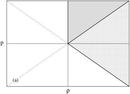
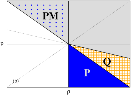
Figure 1: Energy conditions: (a) The shaded regions fulfill the Weak Energy Condition (WEC): $\rho\geq 0$ and $\rho+p\geq 0$. The lighter-shaded one also satisfies the Dominant Energy Condition (DEC): $\rho\geq|p|$; (b) The region shaded in gray (with or without dots) fulfills the Strong Energy Condition (SEC): $\rho+p\geq 0$ and $\rho+3p\geq 0$. The quintessence (Q) region ($-1<\omega_{e}<-1/3$) is marked cross-hatched, and the usual phantom region ($\omega_{e}\leq-1$ with $\rho>0$) is indicated by P. The gray-dotted region corresponds to an unusual kind of phantom $\omega_{e}<-1$ with $\rho<0$, which we call “Phantom Matter” (PM). Note that PM satisfies the SEC. The cosmon behaves in many cases as PM within the $\Lambda$XCDM model.

As we have mentioned, experimentally an effective (standard) phantom fluid ($\rho_{D}>0$, $\omega_{e}<-1$) for the DE cannot be discarded at present because it is allowed by the combined analysis of the supernovae and CMB data [5, 13, 14]. In the following we will construct a simple composite model where this kind of mixture situations can be met. The resulting $\Lambda$XCDM model is a kind of “composite XCDM model” because, in contradistinction to the original XCDM [6], we keep both the cosmological term (with a given status of dynamical entity) and also the new dynamical fluid $X$, and we assume that in general they are in interaction . Obviously a negative value of the cosmological term at present ($\Lambda_{0}<0$) is allowed in this framework (with the current total DE density $\rho_{D}>0$) thanks to the $X$ component. We will see that in the future this may cause a halt of the expansion. This issue has been investigated also in models with a fixed negative value of the cosmological term [22]. However, thanks to the variability of $\Lambda$ and/or the PM behavior of $X$, the halt will also be possible for $\Lambda_{0}>0$. The combined dynamics of $\Lambda$ and cosmon $X$ opens many other possibilities that cannot be offered by models which just add up a quintessence field to the standard $\Lambda$CDM and commit to some particular form of the potential for that field. The fact that we do not specify the nature of $X$ by e.g. identifying it with a scalar field, endows our discussion with a higher degree of generality.

It should be stressed right from the start that despite the time variation of the cosmological parameters within our framework, this fact in no way contradicts the general covariance of the theory. This is independent of whether such variation is inherited from RG considerations or it has some general unspecified origin [49, 50]. The parameters could even be variable in space as well (see e.g. [45]), although we will not allow them to do so here because we want to preserve the Cosmological Principle. The general covariance is insured by imposing the fulfillment of the general Bianchi identity on both sides of Einstein’s equations. The kind of particular relations that this identity will imply among the various cosmological quantities will depend on the metric itself, which in our case we choose to be the Friedmann-Lemaître-Robertson-Walker (FLRW) one . The most general form of the Bianchi identity expressing the equation of continuity for a mixture of fluids (1) and variable cosmological parameters reads:

$$\frac{d}{dt}\left[G\,\left(\sum_{i}\rho_{i}\right)\right]+G\,H\,\sum_{i}\alpha_{i}\,\rho_{i}=0\,,\ \ \ \ \ \alpha_{i}\equiv 3(1+\omega_{i})\,.$$ (2)

In our case we assume that we have matter-radiation, $\rho_{m}=\rho_{M}+\rho_{R}$, and two DE components: one is called $X$ (“cosmon”), with dynamical density $\rho_{X}=\rho_{X}(t)$, and the other is a cosmological term with density $\rho_{\Lambda}$, which can be constant but in general it is also allowed to vary with the evolution: $\rho_{\Lambda}=\rho_{\Lambda}(t)$. This is perfectly possible [1] and preserves the Cosmological Principle provided it only varies with the cosmic time or (equivalently) with the cosmological redshift: $\rho_{\Lambda}=\rho_{\Lambda}(z)$. The two DE components have barotropic indices $\omega_{X}$ and $\omega_{\Lambda}=-1$ respectively. In general the index $\omega_{X}$ for the cosmon will be dynamical, but in practice one can assume that $X$ is some barotropic fluid with constant $\omega_{X}$, typically in one of the two expected ranges $\omega_{X}\gtrsim-1$ (quintessence-like) and $\omega_{X}\lesssim-1$ (phantom-like). For the moment we assume it is an arbitrary function of time or redshift. It should be clear that for the “$\Lambda$ fluid” the relation $\omega_{\Lambda}=-1$ holds irrespective of whether $\rho_{\Lambda}$ is strictly constant or variable. In this work we will keep the gravitational coupling $G$ constant and assume that the matter-radiation density $\rho_{m}=\rho_{M}+\rho_{R}$ is conserved. Hence Eq. (2) splits into corresponding conservation laws for matter-radiation and total DE, namely

$$\dot{\rho}_{m}+\,\alpha_{m}\,\rho_{m}\,H=0\,,\ \ \ \ \ \ \alpha_{m}\equiv 3(1+\omega_{m})\,,$$ (3)

with

$$\omega_{m}=\frac{1}{3}\,\frac{\rho_{R}}{\rho_{M}+\rho_{R}}\,,$$ (4)

and

$$\dot{\rho}_{D}+\alpha_{e}\,\rho_{D}\,H=0\,,\ \ \ \ \ \ \alpha_{e}\equiv 3\,(1+\omega_{e})\,,$$ (5)

with

$$\rho_{D}=\rho_{\Lambda}+\rho_{X}.$$ (6)

In Eq.(4) $\omega_{m}=0,1/3\ (\alpha_{m}=3,4)$ for the matter dominated epoch and the radiation dominated epoch respectively. Clearly, the existence of a dynamical DE component $X$ is a necessary condition for $\rho_{\Lambda}$ being variable in this framework. In the particular case where $\rho_{\Lambda}$ is constant, $X$ would be self-conserved, but in general $\rho_{\Lambda}$ and $X$ may interact and therefore they can constitute two different dynamical components of the total DE density (6). The effective barotropic index – or effective EOS parameter (1) – of the $\Lambda$XCDM model is

$$\omega_{e}=\frac{p_{\Lambda}+p_{X}}{\rho_{\Lambda}+\rho_{X}}=\frac{-\rho_{\Lambda}+\omega_{X}\,\rho_{X}}{\rho_{\Lambda}+\rho_{X}}=-1+(1+\omega_{X})\,\frac{\rho_{X}}{\rho_{D}}\,.$$ (7)

As noticed above, even if $X$ is a barotropic fluid with constant $\omega_{X}$ the mixture of $X$ and $\Lambda$ is non-barotropic because $\rho_{X}$ and $\rho_{\Lambda}$ will in general be functions of time or redshift, and so will be $\omega_{e}=\omega_{e}(z)$. We shall compute this function precisely for the $\Lambda$XCDM model under certain dynamical assumptions on the behavior of the cosmological term. From the equations above it is easy to see that the overall DE conservation law (5) can be rewritten as follows:

$$\dot{\rho}_{\Lambda}+\dot{\rho}_{X}+\,\alpha_{X}\,\rho_{X}\,H=0\,,\ \ \ \ \ \alpha_{X}\equiv 3(1+\omega_{X})\,.$$ (8)

For constant $\rho_{\Lambda}$, this law boils down to the self-conservation of the $X$ component,

$$\dot{\rho}_{X}+\,\alpha_{X}\,\rho_{X}\,H=0\,.$$ (9)

For variable $\rho_{\Lambda}$, Eq. (8) shows that the dynamics of the cosmological term and the cosmon become entangled. One can confirm Eq. (8) starting from the total energy-momentum tensor of the mixed DE fluid, with $4$-velocity $U_{\mu}$:

$$T^{D}_{\mu\nu}=T^{\Lambda}_{\mu\nu}+T^{X}_{\mu\nu}=(\rho_{\Lambda}-\omega_{X}\,\rho_{X})\,g_{\mu\nu}+(1+\omega_{X})\rho_{X}\,U_{\mu}\,U_{\nu}\,.$$ (10)

Then one can use the FLRW metric

$$ds^{2}=dt^{2}-a^{2}(t)\left(\frac{dr^{2}}{1-k\,r^{2}}+r^{2}\,d\theta^{2}+r^{2}\,\sin^{2}\theta\,d\phi^{2}\right)$$ (11)

and straightforwardly compute $\bigtriangledown^{\mu}\,{T^{D}}_{\mu\nu}=0$. The result of course is (8). Another fundamental equation of the cosmological model under construction is Friedmann’s equation

$$H^{2}\equiv\left(\frac{\dot{a}}{a}\right)^{2}=\frac{8\pi\,G}{3}\left(\rho_{m}+\rho_{D}\right)-\frac{k}{a^{2}}=\frac{8\pi\,G}{3}\left(\rho_{m}+\rho_{\Lambda}+\rho_{X}\right)-\frac{k}{a^{2}}\,.$$ (12)

Let us also quote the dynamical field equation for the scale factor:

$$\frac{\ddot{a}}{a}=-\frac{4\pi\,G}{3}\,[\rho_{m}\,(1+3\omega_{m})+\rho_{D}\,(1+3\omega_{e})]=-\frac{4\pi\,G}{3}\,[\rho_{m}\,(1+3\omega_{m})-2\,\rho_{\Lambda}+\rho_{X}\,(1+3\omega_{X})]\,.$$ (13)

This one is not independent from (12) and (8), as can be easily seen by computing the time derivative of $H$ with the help of equations (12),(5) and (3):

$$\dot{H}=-\frac{4\pi\,G}{3}[\alpha_{m}\,\rho_{m}+\alpha_{e}\rho_{D}]+\frac{k}{a^{2}}=-\frac{4\pi\,G}{3}\,[\alpha_{m}\,\rho_{m}+\alpha_{X}\rho_{X}]+\frac{k}{a^{2}}\,.$$ (14)

Then Eq.(13) immediately follows from ${\ddot{a}}/{a}=\dot{H}+H^{2}$, showing that indeed it is not independent. However it is useful to have (13) at hand because it exhibits the acceleration law for the scale factor under the combined influence of the matter-radiation density $\rho_{m}$ and the composite DE density (6).

How do we proceed next? Clearly, even if the index $\omega_{X}$ for the cosmon would be given, we have three independent equations, e.g. (3),(8) and (12), but four unknown functions $(H(t),\rho_{m}(t),\rho_{\Lambda}(t),\rho_{X}(t))$. As a matter of fact, Eq.(3) is decoupled from the rest, and its solution in the matter dominated and radiation dominated eras can be cast in the simple unified form

$$\rho_{m}(z)=\rho_{m}^{0}\left(1+z\right)^{\alpha_{m}}\,,$$ (15)

where $\alpha_{m}=3,4$ respectively for each era. For convenience we have expressed this solution in terms of the cosmological redshift, $z$, with the help of $H\,dt=-dz/(1+z)$. Notice that Eq.(5) can also be solved explicitly for the total DE density:

$$\rho_{D}(z)=\rho_{D}^{0}\,\exp\left\{3\,\int_{0}^{z}\,dz^{\prime}\frac{1+\omega_{e}(z^{\prime})}{1+z^{\prime}}\right\}\,.$$ (16)

This equation is basically formal. In practice it cannot be used unless the model is explicitly solved, meaning that we need first to find the individual functions $\rho_{\Lambda}=\rho_{\Lambda}(z)$ and $\rho_{X}=\rho_{X}(z)$ for the two components of the DE. In particular, this equation does not imply that $\rho_{D}=\rho_{D}(z)$ is positive definite for all $z$ because, after solving the model, the function $\omega_{e}=\omega_{e}(z)$ may present singularities at certain values of $z$. The reciprocal relation expressing the effective EOS parameter in terms of the total DE density is

$$\omega_{e}(z)=-1+\frac{1+z}{3}\,\frac{1}{\rho_{D}}\,\frac{d\rho_{D}}{dz}\,.$$ (17)

From (7) and (17) we get

$$\alpha_{X}\,\rho_{X}=\,(1+z)\,\frac{d\rho_{D}}{dz}$$ (18)

which shows that the effective quintessence ($d\rho_{D}/dz>0$) or phantom-like ($d\rho_{D}/dz<0$) character of the $\Lambda$XCDM model will be known once the sign of $\alpha_{X}$ and the sign of the density $\rho_{X}$ of the cosmon field are known. In particular, we note the curious fact that even if $\omega_{X}<-1$ the model could still effectively look as quintessence-like provided we admit the possibility that the cosmon field can have negative energy-density ($\rho_{X}<0$) . In general the $\Lambda$XCDM model effectively behaves as quintessence (resp. phantom DE) if and only if $\alpha_{X}$ and $\rho_{X}$ have the same (resp. opposite) signs.

In the end we see that we have two coupled equations (8) and (12) for three unknowns $(H(t),\rho_{\Lambda}(t),\rho_{X}(t))$. We need a third equation to solve the $\Lambda$XCDM model. Here we could provide either a specific model for $X$ or one for $\rho_{\Lambda}$. Since $X$ represents a generic form of dynamics other than the cosmological term (the scalar fields being just one among many possible options), from our point of view it is more fundamental to provide a model for $\rho_{\Lambda}$. The simplest possibility is to assume $\rho_{\Lambda}=const.$ In this case the new model is a trivial extension of the standard $\Lambda$CDM one, but even in this case it leads to interesting new physics (see scenario I, Section 5). However, in the general case $\rho_{\Lambda}$ could be a dynamical quantity and a most appealing possibility is to link its variability to the renormalization group (RG) [20]. Once the general principles of QFT in curved space-time (or in Quantum Gravity [47]) will determine the RG scaling law for $\Lambda$, the dynamics of $X$ will be tied to the conservation law (8) in a completely model-independent way; that is to say, independent of the ultimate nature of the cosmon entity. This will be true provided we adhere to the commonly accepted Ansatz that the total DE must be a conserved quantity independent of matter. While we do not know for the moment what are the general principles of QFT in connection to the running properties of the cosmological term in Einstein’s equations, we have already some hints which may be put into test. As a guide we will use the cosmological RG model described in [23], based on the framework of  [20, 46] within QFT in curved space-time. A more general RG cosmological model with both running $G$ and running $\rho_{\Lambda}$ can also be constructed within QFT in curved space-time, see Ref.[45]. However, for simplicity hereafter we limit ourselves to the case $G=const.$ Briefly, the model we will use is based on a RG equation for the CT of the general form

$$(4\,\pi)^{2}\,\frac{d\rho_{\Lambda}}{d\ln\mu}=\sum_{n=1}^{\infty}\,A_{n}\,\mu^{2n}\,.$$ (19)

Here $\mu$ is the energy scale associated to the RG running in cosmology. It has been argued that $\mu$ can be identified with the Hubble parameter $\mu=H$ at any given epoch [20]. Since $H$ evolves with the cosmic time, the cosmological term inherits a time-dependence through its primary scale evolution with the renormalization scale $\mu$. Coefficients $A_{n}$ are obtained after summing over the loop contributions of fields of different masses $M_{i}$ and spins $\sigma_{i}$. The general behavior is $A_{n}\sim\sum M_{i}^{4-2n}$  [20, 46]. Therefore, for $\mu\ll M_{i}$, the series above is an expansion in powers of the small quantities $\mu/M_{i}$. Given that $A_{1}\sim\sum M_{i}^{2}$, the heaviest fields give the dominant contribution. This trait (“soft-decoupling”) represents a generalization of the decoupling theorem in QFT– see [23] for a more detailed discussion. Now, since $\mu=H_{0}\sim 10^{-33}\,eV$ the condition $\mu\ll M_{i}$ is amply met for all known particles, and the series on the r.h.s of Eq. (19) converges extremely fast. Only even powers of $\mu=H$ are consistent with general covariance [23], barring potential bulk viscosity effects in the cosmic fluid [53]. The $n=0$ contribution is absent because it corresponds to terms $\propto M_{i}^{4}$ that give an extremely fast evolution. Actually from the RG point of view they are excluded because, as noted above, $\mu\ll M_{i}$ for all known masses. In practice only the first term $n=1$ is needed, with $M_{i}$ of the order of the highest mass available. We may assume that the dominant masses $M_{i}$ are of order of a high mass scale near the Planck mass $M_{P}$. Let us define an effective mass $M$ as the total mass of the heavy particles contributing to the $\beta$-function on the r.h.s. of (19) after taking into account their multiplicities $a_{i}$ [23]:

$$M\equiv\sqrt{\left|\sum_{i}\,a_{i}\,M_{i}^{2}\right|}\,.$$ (20)

We introduce (as in [23]) the ratio

$$\nu=\frac{\sigma}{12\pi}\frac{M^{2}}{M_{P}^{2}}\,.$$ (21)

Here $\sigma=\pm 1$ depending on whether bosons or fermions dominate in their loop contributions to (19). Thus, if the effective mass $M$ of the heavy particles is just $M_{P}$, then $\nu$ takes the canonical value $\sigma\,\nu_{0}$, with

$$\nu_{0}\equiv\frac{1}{12\,\pi}\simeq 2.6\times 10^{-2}\,.$$ (22)

We cannot exclude a priori that $\nu$ can take values above (22) if these multiplicities are very high. Under the very good approximation $n=1$, and with $\mu=H$, Eq. (19) abridges to [23]

$$\frac{d\rho_{\Lambda}}{d\ln H}=\frac{3\,\nu}{4\,\pi}\,M_{P}^{2}\,H^{2}\,.$$ (23)

Equation (23) is the sought-for third equation needed to solve our cosmological model. Its solution is

$$\rho_{\Lambda}=c_{0}+c_{1}\,H^{2}\,,\\$$ (24)

with

$$c_{0}=\rho_{\Lambda}^{0}-\frac{3\,\nu}{8\pi}M_{P}^{2}\,H_{0}^{2}\,,\ \ \ c_{1}=\frac{3\,\nu}{8\pi}\,M_{P}^{2}\,,$$ (25)

where $H=H(t)$ is given by (12). Notice that this result gives some theoretical basis to the original investigation of the possibility that $\Lambda\sim H^{2}$ (equivalently, $\rho_{\Lambda}\sim H^{2}\,M_{P}^{2}$) [1] at the present epoch. However, in our case rather than a law of the type $\rho_{\Lambda}\sim H^{2}\,M_{P}^{2}$ we have $\delta\rho_{\Lambda}\sim H^{2}\,M_{P}^{2}$, and the variation $\delta\rho_{\Lambda}$ around the reference value is controlled by a RG equation.

3 Analytical solution of the $\Lambda$XCDM model

Using (8) (12), (14) and (23) we can present the relevant set of equations of the $\Lambda$XCDM model in terms of the cosmological redshift variable $z$ as follows:

$$\frac{d\,\rho_{X}}{dz}+\frac{d\,\rho_{\Lambda}}{dz}=\frac{\alpha_{X}\,\rho_{X}}{1+z}\,,$$

$$\frac{d\rho_{\Lambda}}{dz}=\frac{3\,\nu}{8\,\pi}\,M_{P}^{2}\,\frac{dH^{2}}{dz}\,,$$

$$\,\frac{dH^{2}}{dz}=\frac{8\,\pi\,G}{3}\,\frac{\alpha_{m}\,\rho_{m}+\alpha_{X}\,\rho_{X}}{1+z}+2\,H_{0}^{2}\,\Omega_{K}^{0}\,(1+z)\,.$$ (26)

The latter can be replaced by Friedmann’s equation (12) at convenience. Here $\Omega_{K}^{0}=-k/H_{0}^{2}$ is the space curvature term at the present time.

Equations (3) must be solved for $(H,\rho_{X},\rho_{\Lambda})$, where $\rho_{m}$ is known from Eq. (15). Instead of $\rho_{\Lambda},\rho_{X}$ we will use

$$\Omega_{\Lambda}(z)=\frac{\rho_{\Lambda}(z)}{\rho_{c}^{0}}\,,\ \ \ \ \ \ \Omega_{X}=\frac{\rho_{X}(z)}{\rho_{c}^{0}},$$ (27)

where $\rho_{c}^{0}=3H^{2}_{0}/8\pi\,G$ is the critical density at present. We also define

$$\Omega_{m}(z)=\frac{\rho_{m}(z)}{\rho_{c}^{0}}\,,\ \ \ \ \Omega_{K}(z)=\Omega_{K}^{0}\,(1+z)^{2}\,.$$ (28)

From these equations we can derive the following differential equation for $\Omega_{X}$:

$$\frac{d\Omega_{X}}{dz}-(1-\nu)\,\frac{\alpha_{X}\,\Omega_{X}}{1+z}=-\nu\,\frac{\alpha_{m}\,\Omega_{m}}{1+z}-2\,\nu\,\Omega_{K}^{0}\,(1+z)\,.$$ (29)

We can solve it for $\Omega_{X}$ exactly, even if $\omega_{X}$ (hence $\alpha_{X}$) is an arbitrary function of the redshift. The result is the following:

$$\Omega_{X}(z)=\Omega_{X}^{0}\,\left[1-\int_{0}^{z}\,dz^{\prime\prime}\,q(z^{\prime\prime})\,\exp{\left\{-\int_{0}^{z^{\prime\prime}}\,dz^{\prime}\,p(z^{\prime})\right\}}\right]\,\exp{\left\{\int_{0}^{z}\,dz^{\prime}\,p(z^{\prime})\right\}}\,,$$ (30)

where

$$p(z)=\frac{\alpha_{X}\,(1-\nu)}{1+z}\,,$$ (31)

$$q(z)=\nu\,\left[\alpha_{m}\,\frac{\Omega_{m}^{0}}{\Omega_{X}^{0}}\,(1+z)^{\alpha_{m}-1}+2\,\frac{\Omega_{K}^{0}}{\Omega_{X}^{0}}\,(1+z)\right]\,.$$

Notice that if $\nu=0$ then $\Omega_{\Lambda}$ is strictly constant, Eq. (29) reduces to Eq. (9) and $\Omega_{X}(z)$ becomes self-conserved, as expected. If, in addition, $\omega_{X}=$const. then (30) collapses at once to

$$\Omega_{X}(z)=\Omega_{X}^{0}\,(1+z)^{\alpha_{X}}\,,$$ (32)

which is of course the solution of (9) for constant $\alpha_{X}$. This situation is the simplest possibility, and we shall further discuss it in Section 5 as a particular case of our more general framework in which the two components of the DE are dynamical and interacting with one another. The next to simplest situation appears when $\nu\neq 0$ (still with $\omega_{X}=$const.) because then there is an interaction between the two components of the DE and these components can be treated as barotropic fluids. In such case we can work out the integrals in (30) and obtain a non-trivial fully analytical solution of the system (3) for arbitrary spatial curvature. The final result can be cast as follows:

$$\frac{H^{2}(z)}{H_{0}^{2}}=\frac{\Omega_{\Lambda}^{0}-\nu}{1-\nu}+F(z)\,,$$

$$\Omega_{\Lambda}(z)=\frac{\Omega_{\Lambda}^{0}-\nu}{1-\nu}+\nu\,F(z)\,,$$

$$\Omega_{X}(z)=(1-\nu)\,F(z)-\Omega_{m}^{0}\,(1+z)^{\alpha_{m}}-\Omega_{K}^{0}\,(1+z)^{2}\,,$$ (33)

with

$$F(z)= \frac{\Omega_{m}^{0}(\alpha_{m}-\alpha_{X})}{\alpha_{m}-\alpha_{X}\,(1-\nu)}\,(1+z)^{\alpha_{m}}-\frac{\,\Omega_{K}^{0}(\alpha_{X}-2)}{2-\alpha_{X}\,(1-\nu)}\,(1+z)^{2}$$ (34)

$$+\left[\frac{1-\Omega_{\Lambda}^{0}}{1-\nu}-\frac{\Omega_{m}^{0}(\alpha_{m}-\alpha_{X})}{\alpha_{m}-\alpha_{X}\,(1-\nu)}+\frac{\,\Omega_{K}^{0}(\alpha_{X}-2)}{2-\alpha_{X}\,(1-\nu)}\right]\,(1+z)^{\alpha_{X}\,(1-\nu)}\,.$$

The solution above corresponds to the matter ($\alpha_{m}=3$) or radiation ($\alpha_{m}=4$) dominated eras. The expansion rate for the $\Lambda$XCDM model in any of these eras can be expressed as

$$H^{2}(z)=H_{0}^{2}\,\left[\Omega_{m}^{0}\,(1+z)^{\alpha_{m}}+\Omega_{K}^{0}\,(1+z)^{2}+\Omega_{D}(z)\,\right]\,,$$ (35)

where $\Omega_{D}(z)=\rho_{D}(z)/\rho_{c}^{0}$ is the total DE energy density in units of the current critical density. From the previous formulae the latter can be written in full as follows:

$$\Omega_{D}(z)= \frac{\Omega_{\Lambda}^{0}-\nu}{1-\nu}-\frac{\nu\,\alpha_{X}\,\Omega_{m}^{0}\,(1+z)^{\alpha_{m}}}{\alpha_{m}-\alpha_{X}\,(1-\nu)}-\frac{\nu\,\alpha_{X}\,\Omega_{K}^{0}\,(1+z)^{2}}{2-\alpha_{X}\,(1-\nu)}$$ (36)

$$+\left[\frac{1-\Omega_{\Lambda}^{0}}{1-\nu}-\frac{\Omega_{m}^{0}(\alpha_{m}-\alpha_{X})}{\alpha_{m}-\alpha_{X}\,(1-\nu)}+\frac{\,\Omega_{K}^{0}(\alpha_{X}-2)}{2-\alpha_{X}\,(1-\nu)}\right]\,(1+z)^{\alpha_{X}\,(1-\nu)}\,.$$

Let us finally derive the generalized form of the “cosmic sum rule” within the $\Lambda$XCDM model. From (36) we can readily verify that for $z=0$ we have $\Omega_{D}(0)=1-\Omega_{M}^{0}-\Omega_{K}^{0}$. This renders the desired sum rule satisfied by the current values of the cosmological parameters in the $\Lambda$XCDM:

$$\Omega_{M}^{0}+\Omega_{D}^{0}+\Omega_{K}^{0}=\Omega_{M}^{0}+\Omega_{\Lambda}^{0}+\Omega_{X}^{0}+\Omega_{K}^{0}=1\,.$$ (37)

The cosmic sum rule can be extended for any redshift

$$\tilde{\Omega}_{m}(z)+\tilde{\Omega}_{\Lambda}(z)+\tilde{\Omega}_{X}(z)+\tilde{\Omega}_{K}(z)=1\,,$$ (38)

provided we define the new cosmological functions

$$\tilde{\Omega}_{m}(z)=\frac{\rho_{m}(z)}{\rho_{c}(z)}\,,\ \ \tilde{\Omega}_{\Lambda}(z)=\frac{\rho_{\Lambda}(z)}{\rho_{c}(z)}\,,\ \ \tilde{\Omega}_{X}(z)=\frac{\rho_{X}(z)}{\rho_{c}(z)},\ \ \tilde{\Omega}_{K}(z)=-\frac{k}{H^{2}(z)}\,(1+z)^{2}\,,$$ (39)

with $\rho_{c}(z)=3H^{2}(z)/8\pi\,G$ the critical density at redshift $z$. These functions should not be confused with (27) and (28). We will, however, use more frequently the latter.

We may ask ourselves: in which limit do we recover the standard $\Lambda$CDM model? We first notice that for $\nu=0$ the function (34) dwarfs to

$$F(z)=\Omega_{m}^{0}\,(1+z)^{\alpha_{m}}+\Omega_{K}^{0}\,(1+z)^{2}+\Omega_{X}^{0}\,(1+z)^{\alpha_{X}}\,.$$ (40)

where we have used (37). Then substituting this in (3) one can immediately check that the standard $\Lambda$CDM model formulae are obtained from those of the $\Lambda$XCDM model in the limit $\nu\rightarrow 0$ and $\Omega_{X}^{0}\rightarrow 0$, as could be expected.

4 Nucleosynthesis constraints and the evolution of the DE from the radiation era into the matter dominated epoch

At temperatures near $1\,MeV$ the weak interactions (responsible for neutrons and protons to be in equilibrium) freeze-out. The expansion rate is sensitive to the amount of DE, and therefore primordial nucleosynthesis ($T\sim 0.1-1\,MeV$) can place stringent bounds on the parameters of the $\Lambda$XCDM model. A similar situation was considered in the running cosmological models previously studied in Ref. [23, 37]. In the latter, nucleosynthesis furnished a bound on the parameter $\nu$ defined in Eq.(21) from the fact that the ratio of the cosmological constant density to the matter density should be relatively small at the nucleosynthesis epoch, $(\rho_{\Lambda}/\rho_{m})_{N}\ll 1$, of order $10\%$ (see also [54]). This condition led to $\nu<0.1$, which is e.g. amply satisfied by the natural value (22). However, in the $\Lambda$XCDM model the total DE density is not just $\rho_{\Lambda}$, but $\rho_{D}$ given by (6), and moreover the dynamics of the cosmological term here is not linked to the matter density (as in Ref.[23]) but to the cosmon density. Therefore, the appropriate ratio to be defined in the present instance is

$$r\equiv\frac{\rho_{D}}{\rho_{m}}=\frac{\rho_{\Lambda}+\rho_{X}}{\rho_{m}}=\frac{\Omega_{\Lambda}+\Omega_{X}}{\Omega_{m}}\,.$$ (41)

Notice that for the flat case ($k=0$) this ratio is related to $\tilde{\Omega}_{D}\equiv\tilde{\Omega}_{\Lambda}+\tilde{\Omega}_{X}$ (cf. Eq.(39)) as follows:

$$\tilde{\Omega}_{D}=\frac{r}{1+r}\,.$$ (42)

Even if $k\neq 0$, at the nucleosynthesis time the curvature term is negligible. Therefore the nucleosynthesis bounds on $\tilde{\Omega}_{D}$ of order $10\%$ [54] are essentially bounds on $r$. Let us compute the ratio $r$ in general and then evaluate it at nucleosynthesis. For convenience let us use the function (34) and express the result as

$$r(z)=\frac{\frac{\Omega_{\Lambda}^{0}-\nu}{1-\nu}+F(z)-\Omega_{m}^{0}\,(1+z)^{\alpha_{m}}-\Omega_{K}^{0}\,(1+z)^{2}}{\Omega_{m}^{0}(1+z)^{\alpha_{m}}}\,.$$ (43)

It is easy to check that for $z=0$ this equation reduces to the expected result

$$r_{0}\equiv r(0)=\frac{\Omega_{\Lambda}^{0}+\Omega_{X}^{0}}{\Omega_{M}^{0}}=\frac{\Omega_{D}^{0}}{\Omega_{M}^{0}}\,.$$ (44)

Let now $z_{N}\sim T_{N}/T_{0}\sim(0.1\,MeV)/(2\times 10^{-4}\,eV)\sim 10^{9}$ be the typical cosmological redshift at nucleosynthesis time. Let also $\omega_{R}=1/3$ and $\alpha_{R}=4$ be the values of the parameters $\omega_{m}$ and $\alpha_{m}$ at nucleosynthesis (and in general in the radiation epoch). We can obviously neglect the first (constant) term in the numerator of (43) at $z=z_{N}$, and as we have said also the contribution from the spatial curvature (which scales with two powers less of $(1+z)$ as compared to the radiation density). After a straightforward calculation we obtain

$$r_{N}\equiv r(z_{N})\simeq\frac{F(z_{N})-\Omega_{R}^{0}\,(1+z_{N})^{4}}{\Omega_{R}^{0}(1+z_{N})^{4}}=r_{\epsilon}+R_{N}(z_{N})$$ (45)

where

$$r_{\epsilon}\equiv-\frac{\epsilon}{\omega_{R}-\omega_{X}+\epsilon}\,,$$ (46)

with

$$\epsilon\equiv\,\nu\,(1+\omega_{X})\,,$$ (47)

and we have defined the function

$$R_{N}(z_{N})=\left[\frac{1-\Omega_{\Lambda}^{0}}{\Omega_{R}^{0}(1-\nu)}-\frac{\omega_{R}-\omega_{X}}{\omega_{R}-\omega_{X}+\epsilon}-\frac{\Omega_{K}^{0}}{\Omega_{R}^{0}}\,\frac{1+3\,\omega_{X}}{1+3\,\omega_{X}-3\,\epsilon}\right]\,(1+z_{N})^{3\,(\omega_{X}-\epsilon)-1}\,.$$ (48)

Here $\Omega_{R}^{0}$ is the radiation density at present. The parameter $\epsilon$ defined in (47) will soon play an important role in our discussion. The “residual” function (48) will be totally harmless at nucleosynthesis provided the exponent of $(1+z_{N})$ that goes with it is sufficiently large (in absolute value) and negative, in which case $R_{N}(z_{N}\sim 10^{9})$ will be negligible. We start with the condition that it be negative, which provides the constraint

$$\omega_{X}-\epsilon<\frac{1}{3}\,.$$ (49)

However, there is also the first term on the r.h.s. of (45). This term does not decay with the redshift, it is constant and therefore must be small by itself. If we take the same condition as in [23] concerning the bound on the ratio of DE density to radiation density at nucleosynthesis, namely $|r_{N}|<10\%$, we find the additional constraint

$$\left|r_{\epsilon}\right|=\left|\frac{\epsilon}{\omega_{R}-\omega_{X}+\epsilon}\right|<0.1\,\,.$$ (50)

We shall assume that the cosmon barotropic index lies in the interval

$$-1-\delta/3<\omega_{X}<-1/3\ \ \ \ (\delta>0)\,,$$ (51)

with $\delta$ a small positive quantity. The upper limit is fixed by requiring that $X$ has at most quintessence behavior (i.e. excluding matter-radiation behavior); the lower limit is expected to be some number below (but around) $-1$ in order to accommodate a possible phantom-like behavior. From Eq. (51), and recalling that $\omega_{R}=1/3$, it is patent that the bound (50) just translates into a rough bound on $\epsilon$ itself:

$$|r_{\epsilon}|\simeq|\epsilon|=|\nu\,(1+\omega_{X})|<0.1\,.$$ (52)

Using this relation and the condition (51) we see that the previous bound (49) is amply satisfied and the function (48) actually behaves as

$$R_{N}(z)\sim(1+z)^{\beta}\ \ \ \ \ (\beta<-2-3\,\epsilon)\,.$$ (53)

This means that $R_{N}(z_{N}\sim 10^{9})$ will be completely negligible, as desired. Therefore, the two bounds from nucleosynthesis just reduce to one, Eq. (50), and we can simply set there $|r_{N}|=|r_{\epsilon}|$. We will use the exact bound (50) for our numerical analysis, but the approximate version (52) is useful for qualitative discussions.

In contrast to the nucleosynthesis bound obtained in Ref. [23] for the alternative scenario where the DE was composed only of a running cosmological constant (in interaction with matter) we see that for the $\Lambda$XCDM model it is not necessary to require that $|\nu|$ is small, but only the product of $|\nu|$ times $|\alpha_{X}|$. We also note that in the $\Lambda$XCDM model for $\nu\neq 0$ there is an irreducible contribution of the DE to the total energy density in the radiation era, whose size is basically fixed by the tolerance of the nucleosynthesis processes to the presence of a certain amount of dark energy. The existence of this residual constant contribution shows that in the $\Lambda$XCDM model the presence of the DE component takes place at all epochs of the Universe evolution. It is therefore interesting to study what will be the evolution of this tiny (but not necessarily negligible) contribution in later times, in particular in the matter dominated epoch, where $\omega_{m}=0$ ($\alpha_{m}=3$). Let us thus compute the ratio (41) in this epoch, and call it $r_{M}(z)$. In this case we apply the full formula (43), without neglecting any term, because $z$ in the matter-dominated epoch covers a range from $\sim 10^{3}$ to (near) $-1$. The final result is:

$$r_{M}(z)=\frac{\Omega_{\Lambda}^{0}-\nu}{(1-\nu)\,\Omega_{M}^{0}\,(1+z)^{3}}+\frac{\Omega_{K}^{0}}{\Omega_{M}^{0}}\,\frac{3\,\epsilon}{(1+3\,\omega_{X}-3\,\epsilon)\,(1+z)}+\frac{\epsilon}{\omega_{X}-\epsilon}+R_{M}(z)\,,$$ (54)

with

$$R_{M}(z)=\left[\frac{1-\Omega_{\Lambda}^{0}}{\Omega_{M}^{0}(1-\nu)}-\frac{\omega_{X}}{\omega_{X}-\epsilon}-\frac{\Omega_{K}^{0}}{\Omega_{M}^{0}}\,\frac{1+3\,\omega_{X}}{1+3\,\omega_{X}-3\,\epsilon}\right]\,(1+z)^{3\,(\omega_{X}-\epsilon)}\,.$$ (55)

It is easy to check that for $z=0$ the expression (54) shrinks just to (44). For general $z$ we see that the first term on the r.h.s. of (54) goes like $(1+z)^{-3}$ and hence evolves fast with the expansion and is unbounded for $z\rightarrow-1$. The second term (the curvature dependent term) evolves much more slowly, namely as $(1+z)^{-1}$ and it can be neglected to study the future evolution (also because $\Omega_{K}^{0}$ is very small). The rising of $r(z)$ with the expansion cannot be stopped in the standard $\Lambda$CDM model because for it the ratio just reads

$$r_{M}(z)=\frac{\Omega_{\Lambda}^{0}}{\,\Omega_{M}^{0}\,(1+z)^{3}}\,.$$ (56)

This particular result is of course recovered from (54) in the limit $\nu=0$ and $\Omega_{X}^{0}=0$ (see Section 3). However, in the $\Lambda$XCDM the presence of the non-trivial function $R_{M}(z)\sim(1+z)^{3\,(\omega_{X}-\epsilon)}$ is crucial as it allows the existence of both a stopping point, $z_{s}$, as well as of an extremum of the function (54) at some $z=z_{\rm max}$ during the future Universe evolution. We will study the relationship between these two features in the next section and we will see that the stopping condition is correlated with this extremum being a maximum. Here we will concentrate on the conditions of existence of this maximum of $r_{M}(z)$.

Let us from now on restrict our considerations to the flat space case, which is the most favored one. The redshift position $z_{\rm max}$ of the maximum can be worked out from Eq. (54). The result is the following:

$$1+z_{\rm max}=\left[\frac{\Omega_{\Lambda}^{0}-\nu}{\omega_{X}\,(\Omega_{X}^{0}+\nu\,\Omega_{M}^{0})-\epsilon\,(1-\Omega_{\Lambda}^{0})}\right]^{\frac{1}{3\,(1+\omega_{X}-\epsilon)}}\,.$$ (57)

The nature of this extremum is obtained by working out the second derivative of $r(z)$ at $z=z_{\rm max}$. We find

$$r^{\prime\prime}(z_{\rm max})=\frac{3\,\alpha_{X}}{(1+z_{\rm max})^{5}}\,\frac{\Omega_{\Lambda}^{0}-\nu}{\Omega_{M}^{0}}\,,$$ (58)

where $z_{\rm max}$ is given by (57). A sufficient condition for the extremum to be a maximum is that

$$\alpha_{X}\,\left(\Omega_{\Lambda}^{0}-\nu\right)<0\,.$$ (59)

The height of the maximum, $r_{\rm max}\equiv r(z_{\rm max})$, is the following:

$$r_{\rm max}=\frac{1}{(1+z_{\rm max})^{3}}\,\frac{\Omega_{\Lambda}^{0}-\nu}{\Omega_{M}^{0}}\,\frac{1+\omega_{X}}{\omega_{X}-\epsilon}+\frac{\epsilon}{\omega_{X}-\epsilon}\,,$$ (60)

where the last term on the r.h.s. is negligible.

Notice that the aforementioned maximum can only exist in the future (or at present), but not in the past. Its existence in the past would be incompatible with the experimentally confirmed state of acceleration of the Universe that started in relatively recent times. To prove this, one can show that the acceleration Eq. (13) can be written in terms of the ratio (41) and its derivative $r^{\prime}(z)$ with respect to redshift as follows. We first write Friedmann’s equation for $k=0$ in the form $H^{2}=({8\pi\,G}/{3})\,(1+r)\,\rho_{m}$. Then we differentiate it with respect to the cosmic time,

$$\dot{H}=-\frac{4\pi\,G}{3}\left[(1+r)\,\alpha_{m}-\frac{\dot{r}}{H}\right]\,\rho_{m}\,,$$ (61)

where use has been made of the equation of continuity (3). With the help of these equations we compute ${\ddot{a}}/{a}=\dot{H}+H^{2}$:

$$\frac{\ddot{a}}{a} = -\frac{4\pi\,G}{3}\,\left[(1+3\omega_{m})(1+r(t))-\frac{\dot{r}(t)}{H})\right]\,\rho_{m}$$ (62)

$$= -\frac{4\pi\,G}{3}\,\left[(1+3\omega_{m})(1+r(z))+(1+z)\,r^{\prime}(z)\right]\,\rho_{m}\,,$$

where $r^{\prime}(z)=dr(z)/dz$. The last equation shows that if the maximum could take place at some point $z=z_{1}>0$ in the recent past, then any $z$ in the interval $0<z<z_{1}$ would satisfy $r^{\prime}(z)>0$, and then Eq. (62) would immediately imply $\ddot{a}<0$, which is incompatible with the known existence of the acceleration period in our recent past (q.e.d.).

Therefore, the maximum will in general lie ahead in time. After surpassing $z=z_{\rm max}$ into the future, the ratio (54) drops fast (in redshift units) to $r_{M}(z_{s})=-1$, where $z_{s}$ can be relatively close to $-1$. At this point $\rho_{D}$ takes the negative value $\rho_{D}(z_{s})=-\rho_{M}^{0}\,(1+z_{s})^{3}$, with $|\rho_{D}(z_{s})|\ll\rho_{D}^{0}\$. From the previous considerations it is clear that the maximum (57) can only exist for

$$\frac{\Omega_{\Lambda}^{0}-\nu}{\omega_{X}\,(\Omega_{X}^{0}+\nu\,\Omega_{M}^{0})-\epsilon\,(1-\Omega_{\Lambda}^{0})}>0\,.$$ (63)

We point out that if the cosmon $X$ would behave as another pure cosmological term (namely $\omega_{X}=-1$) then $\epsilon=0$ and the maximum (57) would not exist. On the other hand, for $\nu=0$ then again $\epsilon=0$, and for $\omega_{X}\neq-1$ the maximum still exists and is located at

$$1+z_{\rm max}=\left[\frac{\Omega_{\Lambda}^{0}}{\omega_{X}\,\Omega_{X}^{0}}\right]^{\frac{1}{\alpha_{X}}}\ \ \ \ (\nu=0)\,.$$ (64)

Since $\omega_{X}<0$ this enforces $\Omega_{\Lambda}^{0}$ and $\Omega_{X}^{0}$ to have opposite signs.

The various scenarios will be further discussed in the next section from a more general point of view, where we will link the conditions for the stopping of the Universe’s expansion with the conditions of existence of the maximum of (54) before reaching the turning point. The presence of these two points is a central issue in our discussion of the cosmological coincidence problem within the $\Lambda$XCDM . The numerical analysis displaying these features is presented in Section 7. But before that, let us take a closer look to the analytical results and their interpretation.

5 Cosmological scenarios in the $\Lambda$XCDM model. Autonomous system.

For a better understanding of the solution that we have found in Section 3 it will be useful to look at the set of equations (3) from the point of view of the qualitative methods for systems of differential equations. This should help in the interpretation of the numerical analysis performed in Section 7. As a matter of fact, we will end up by solving quantitatively the problem with this alternate method and use it as a cross-check. Again it will simplify our analysis if we assume that the cosmon is a barotropic fluid with $\omega_{X}=$ const. Let us introduce the convenient variable

$$\zeta=-\ln(1+z)\,.$$ (65)

In this variable the remote past ($t=0$) lies at $\zeta=-\infty$ whereas the remote future ($t=\infty$) is at $\zeta=+\infty$. In the previous section we have solved the $\Lambda$XCDM cosmological model exactly for any value of the spatial curvature, but in practice we will set the curvature parameter $\Omega_{K}^{0}$ to zero to conform with the small value suggested by the present observations [3, 5]. This will allow us to deal with the basic set of equations (3) as an autonomous linear system of differential equations in the variable (65). Indeed, after a straightforward calculation we find

$$\frac{d\Omega_{X}}{d\zeta}=-\left[\nu\,\alpha_{m}+(1-\nu)\,\alpha_{X}\right]\,\Omega_{X}-\nu\,\alpha_{m}\,\Omega_{\Lambda}+\nu\,\alpha_{m}\,\Omega_{c}\,,$$

$$\frac{d\Omega_{\Lambda}}{d\zeta}=\nu\,(\alpha_{m}-\alpha_{X})\,\Omega_{X}+\nu\,\alpha_{m}\,\Omega_{\Lambda}-\nu\,\alpha_{m}\,\Omega_{c}\,,$$

$$\,\frac{d\Omega_{c}}{d\zeta}=(\alpha_{m}-\alpha_{X})\,\Omega_{X}+\,\alpha_{m}\,\Omega_{\Lambda}-\alpha_{m}\,\Omega_{c}\,,$$ (66)

where we have defined $\Omega_{c}(z)=\rho_{c}(z)/\rho_{c}^{0}$. Notice that by virtue of (38)

$$\Omega_{m}(z)+\Omega_{\Lambda}(z)+\Omega_{X}(z)=\Omega_{c}(z)\,.$$ (67)

We have actually used this equation to eleminate $\Omega_{m}$ from (5). The matrix of the system (5) has zero determinant. The eigenvalues read

$$\lambda_{1}=-\alpha_{X}\,(1-\nu)\,,\ \ \lambda_{2}=-\alpha_{m}\,,\ \ \ \lambda_{3}=0\,.$$ (68)

The corresponding eigenvectors (up to a constant) are

$${\bf v_{1}}=\begin{pmatrix}1-\nu\\ \nu\\ 1\end{pmatrix}\,,\ \ \ {\bf v_{2}}=\begin{pmatrix}\frac{-\nu\,\alpha_{m}}{\alpha_{m}-\alpha_{X}}\\ \nu\\ 1\end{pmatrix}\,,\ \ \ {\bf v_{3}}=\begin{pmatrix}0\\ 1\\ 1\end{pmatrix}\,.$$ (69)

If we define the column vector

$${\bf\Omega}(\zeta)=\begin{pmatrix}\Omega_{X}(\zeta)\\ \Omega_{\Lambda}(\zeta)\\ \Omega_{c}(\zeta)\end{pmatrix}$$ (70)

then the solution of the autonomous system (5) reads

$${\bf\Omega}(\zeta)=C_{1}\,{\bf v_{1}}\,e^{\lambda_{1}\,\zeta}+C_{2}\,{\bf v_{2}}\,e^{\lambda_{2}\,\zeta}+C_{3}\,{\bf v_{3}}\,,$$ (71)

with

$$C_{1}=\frac{1-\Omega_{\Lambda}^{0}}{1-\nu}-\frac{\Omega_{m}^{0}(\alpha_{m}-\alpha_{X})}{\alpha_{m}-\alpha_{X}\,(1-\nu)}\,,\ \ C_{2}=\frac{\Omega_{m}^{0}(\alpha_{m}-\alpha_{X})}{\alpha_{m}-\alpha_{X}\,(1-\nu)}\,,\ \ C_{3}=\frac{\Omega_{\Lambda}^{0}-\nu}{1-\nu}\,.$$ (72)

The values of these coefficients are fixed by the boundary condition

$${\bf\Omega}(\zeta=0)=\begin{pmatrix}\Omega_{X}^{0}\\ \Omega_{\Lambda}^{0}\\ \Omega_{c}^{0}\end{pmatrix}\,.$$ (73)

One can check that the solution obtained by this method is completely consistent with the one obtained in Section 3 for the flat space case.

Once the solution is expressed in terms of the eigenvalues, as in (71), we can investigate the qualitative behaviour of the dynamical system. Let us describe some possible scenarios for the phase trajectories. Let us recall that the cosmon barotropic index lies in the interval (51). Equivalently,

$$-\delta<\alpha_{X}<2<\alpha_{m}\,\ \ \ \ \ \ (\delta>0)\,.$$ (74)

The scenarios that we wish to consider are mainly the ones that are compatible with the existence of a stopping point in the future Universe expansion. The reason for this is that if there is a stopping point then we can argue (see below) that it can provide an explanation for the cosmic coincidence problem. Of course, this “stopping point” is actually a “turning point”, meaning that the Universe ceases its expansion there, but it subsequently reverses its evolution (then contraction) towards the Big Crunch. Among the possible cosmological scenarios let us remark the following:

• I) $0<\alpha_{X}<2$ and $\nu=0$. In this case the two non-vanishing eigenvalues are both negative, $\lambda_{1}<0\,,\lambda_{2}<0$, meaning that there is an asymptotically stable node. All phase trajectories of the system in vector space (70) become attracted (as $\zeta\rightarrow\infty$) towards the vector node

  $${\bf\Omega}^{*}_{I}=\begin{pmatrix}0\\ \Omega_{\Lambda}^{0}\\ \Omega_{\Lambda}^{0}\end{pmatrix}\,.$$ (75)

  For $\Omega_{\Lambda}^{0}>0$ this fixed point is obviously de Sitter space-time. However, if we further impose the condition $\Omega_{\Lambda}^{0}<0$, the convergence to that node will be stopped because the third component of the vector solution (70), $\Omega_{c}(z)=\rho_{c}(z)/\rho_{c}^{0}=H^{2}(z)/H_{0}^{2}$, cannot become negative. The interpretation of this case is clear: we are in a situation where we have a quintessence cosmon entity $X$ ($-1<\omega_{X}<-1/3$), with density (32), superimposed on a strictly constant cosmological term:

  $$\Omega_{D}(z)=\Omega_{\Lambda}^{0}+\Omega_{X}^{0}\,(1+z)^{\alpha_{X}}\,.$$ (76)

  The requirement $\Omega_{\Lambda}^{0}<0$ eventually stops the Universe expansion at some point in the future because the $X$ density gradually diminishes with the cosmic time and the r.h.s. of (35) becomes zero. We remark that the possibility that $\Omega_{\Lambda}^{0}<0$ should not be discarded a priori. Even though it is clearly unfavored by measurements within the standard $\Lambda$CDM model [2, 3, 4, 5], it is perfectly possible within the $\Lambda$XCDM whose generalized cosmic sum rule (37) for flat space reads

  $$\Omega_{M}^{0}+\Omega_{\Lambda}^{0}+\Omega_{X}^{0}=1\,.$$ (77)

  For example, if we take the approximate prior $\Omega_{M}^{0}=0.3$ (typically from the LSS inventory of matter obtained from galaxy clusters analysis [4]), then a value $\Omega_{\Lambda}^{0}<0$ can be easily compensated for by a positive cosmon density at present: $\Omega_{X}^{0}>0$. Notice that the measurements of distant supernovae and CMB should in principle be sensitive to the total DE content $\Omega_{D}=\Omega_{\Lambda}+\Omega_{X}$, and of course to the total matter content. Moreover, being $\alpha_{X}>0$ we see that $\Omega_{\Lambda}^{0}<0$ is compatible with the existence of the maximum of $r(z)$ at $z=z_{\rm max}$ – cf. Eq.(59).

• II) $-\delta<\alpha_{X}<0$ and $\nu=0$. Here the non-vanishing eigenvalues are of different sign: $\lambda_{1}>0\,,\lambda_{2}<0$. It follows that (75) becomes a saddle point and the phase trajectories depart from it more and more with the evolution. Equation (76) still holds in this case, and for $\Omega_{X}^{0}>0$ the cosmon density increases indefinitely with the expansion. In fact, $X$ behaves here as a standard phantom field (cf. Fig.1) and produces a super-accelerated expansion beyond the normal de Sitter expansion. In these conditions the Universe’s evolution strips apart gravitationally bound objects (and ultimately all bound systems), i.e. it ends up in a frenzy “Big Rip” [15]. However, if $\Omega_{X}^{0}<0$ the r.h.s. of (35) eventually becomes zero and the Universe stops its expansion at some point in the future. We can also see these features in terms of Eq.(71). The sign of the coefficient $C_{1}$ determines in this case whether there can be stopping ($C_{1}<0$) or not ($C_{1}>0$). Since $\nu=0$ here, we have $C_{1}=1-\Omega_{\Lambda}^{0}-\Omega_{M}^{0}=\Omega_{X}^{0}$ and therefore it is the sign of $\Omega_{X}^{0}$ that controls the stopping along the lines mentioned above. Notice that although $\omega_{X}<-1$, the Big Rip is impossible for $\Omega_{X}^{0}<0$ because the term $-\rho_{X}\,(1+3\omega_{X})$ on the r.h.s. of (13) is negative, therefore the cosmon in this instance actually collaborates with matter to enhance more and more the cosmological deceleration until the Universe reaches a turning point. In this case the cosmon $X$ acts as “Phantom Matter” (PM), the only component of the DE that still preserves the SEC (see Fig 1). We stress that even though $X$ behaves as PM here, the sign of the product $\alpha_{X}\,\rho_{X}$ is positive and hence the effective behavior of the $\Lambda$XCDM model remains quintessence-like – see Eq.(18).

• III) $\alpha_{X}=0$ and $\nu\neq 0$. Two eigenvalues are zero ($\lambda_{1}=\lambda_{3}=0$) and $\lambda_{2}<0$. One can check that the following node is the end point of all trajectories:

  $${\bf\Omega}^{*}_{III}(\nu)=\begin{pmatrix}\Omega_{X}^{0}+\nu\,\Omega_{M}^{0}\\ \Omega_{\Lambda}^{0}-\nu\,\Omega_{M}^{0}\\ 1-\Omega_{M}^{0}\end{pmatrix}\,.$$ (78)

  This situation corresponds to effectively having two variable “$\Lambda$’s”, one is $X$ (which has EOS parameter $\omega_{X}=-1$) and the other is $\Lambda$. Both “$\Lambda$’s” are variable because $\nu\neq 0$, but the sum $\rho_{\Lambda}(z)+\rho_{X}(z)=const.$ i.e. $\rho_{D}(z)$ behaves as a strictly constant cosmological term – cf. Eq. (8). With $\Omega_{M}^{0}<1$, there is no possibility for stopping the expansion under these circumstances, no matter how $\Lambda$ varies, because $\Omega_{c}(z)$ (hence $H^{2}(z)$) remains always positive. Although this case is uninteresting for our purposes, it shows at least that there is no turning point in the Universe evolution if the cosmon has the exact EOS of a cosmological term. In Section 4 we also proved that under these circumstances there is no maximum of $r=\rho_{D}/\rho_{m}\,$ either. The Universe moves asymptotically towards an ever-expanding de Sitter phase characterized by an effective cosmological constant given by $\Omega_{\Lambda}^{0}+\Omega_{X}^{0}=1-\Omega_{M}^{0}>0$. We conclude that a necessary condition for the existence of a turning point in the $\Lambda$XCDM model is that the cosmon EOS parameter is different from $-1$; in other words, $\alpha_{X}=0$ is to be excluded from Eq. (74). This will be understood implicitly hereafter.

• IV) $0<\alpha_{X}<2$ and $\nu<1$ (including of course $\nu<0$). As in case I above the two eigenvalues are both negative $\lambda_{1}<0\,,\lambda_{2}<0$ and there is a ($\nu$-dependent) node onto which all phase trajectories are attracted, namely

  $${\bf\Omega}^{*}_{IV}(\nu)=\begin{pmatrix}0\\ \frac{\Omega_{\Lambda}^{0}-\nu}{1-\nu}\\ \frac{\Omega_{\Lambda}^{0}-\nu}{1-\nu}\end{pmatrix}\,.$$ (79)

  For $\nu=0$, ${\bf\Omega}^{*}_{IV}(0)={\bf\Omega}^{*}_{I}$ and we recover the case I above. Again the attraction towards the node can be stopped under suitable conditions. In this case we have to require that

  $$\frac{\Omega_{\Lambda}^{0}-\nu}{1-\nu}<0\ \ \ \ \Rightarrow\ \ \Omega_{\Lambda}^{0}<\nu<1\,.$$ (80)

  Being $\alpha_{X}>0$ we see that this choice is compatible with the existence of the maximum at $z_{\rm max}$, see Eq.(59). In contrast to scenario I, we find that to achieve stopping it is not necessary that $\Omega_{\Lambda}^{0}<0$. This novel trait appears thanks to the non-vanishing interaction between the two components of the DE in the $\Lambda$XCDM, which is gauged by the parameter $\nu$ – as seen from the first two equations in (3). Therefore, we conclude that for quintessence-like cosmon we can have stopping of the expansion not only for $\Omega_{\Lambda}^{0}<0$ but also for $0<\Omega_{\Lambda}^{0}<\nu<1$.

• V) $0<\alpha_{X}<2$ and $\nu=1$. In this case we have the same eigenvalues as in scenario III, but the situation is different. The asymptotic node for the trajectories is

  $${\bf\Omega}^{*}_{V}(\nu)=\begin{pmatrix}1-\Omega_{\Lambda}^{0}\\ \Omega_{\Lambda}^{0}-\Omega_{M}^{0}\,(1-\alpha_{X}/\alpha_{m})\\ 1-\Omega_{M}^{0}\,(1-\alpha_{X}/\alpha_{m})\end{pmatrix}\,.$$ (81)

  Using the sum rule (37) it is easy to see that for $\alpha_{X}=0$ this fixed point coincides with (78) for $\nu=1$, as it should. In contrast to scenario III, in this case the stopping is in principle possible by requiring that the third component of (81) becomes negative. This condition yields

  $$\alpha_{X}<\frac{\Omega_{M}^{0}-1}{\Omega_{M}^{0}}\ \alpha_{m}\,.$$ (82)

  Using $\alpha_{m}=3$ for the matter-dominated epoch and the prior $\Omega_{M}^{0}=0.3$, we find $\alpha_{X}<-7$ (i.e. $\omega_{X}<-1.33$) to achieve stopping. This would be no problem, were it not because the nucleosynthesis constraint derived in Section 4 forbids that the product $|\nu\,\alpha_{X}|$ is too large as in the present case. So this scenario is actually ruled out by nucleosynthesis considerations.

• VI) $0<\alpha_{X}<2$ and $\nu>1$. Here one eigenvalue is positive and the other negative ($\lambda_{1}>0\,,\lambda_{2}<0$) as in scenario II. Therefore the point (75) is again a saddle point from which all trajectories diverge as $\zeta\rightarrow\infty$. This runaway, however, can be stopped provided $C_{1}<0$ in (71). Indeed, since the eigenvector ${\bf v_{1}}$ defines a runaway direction the third component of (71) will eventually become negative, which is the condition for stopping. In the absence of the nucleosynthesis constraint (52), the condition $C_{1}<0$ would be a bit messy, but thanks to this condition we have in good approximation

  $$C_{1}=\frac{1-\Omega_{\Lambda}^{0}}{1-\nu}-\frac{\Omega_{M}^{0}(\omega_{m}-\omega_{X})}{\omega_{m}-\omega_{X}+\epsilon}\simeq\frac{1-\Omega_{\Lambda}^{0}}{1-\nu}-\Omega_{M}^{0}\,,$$ (83)

  and

  $$C_{2}=\frac{\Omega_{M}^{0}(\omega_{m}-\omega_{X})}{\omega_{m}-\omega_{X}+\epsilon}\simeq\Omega_{M}^{0}\,.$$ (84)

  Thus, within this approximation, the stopping condition for this case is

  $$C_{1}<0\ \ \ \ \Longleftrightarrow\ \ \ \frac{1-\Omega_{\Lambda}^{0}}{1-\nu}<\Omega_{M}^{0}\,,$$ (85)

  where $\epsilon$ – defined in (47) – is assumed to be small to satisfy the nucleosynthesis constraint. In the present instance, since we assume $\nu>1$ we have to compensate it with small enough $\alpha_{X}$. The condition (85) is satisfied by choosing

  $$\Omega_{\Lambda}^{0}<1+(\nu-1)\,\Omega_{M}^{0}\,.$$ (86)

  This value could still perfectly lie in the preferred range of values for $\Omega_{\Lambda}^{0}$ near the standard flat $\Lambda$CDM model, i.e. $\Omega_{\Lambda}^{0}\simeq 0.7$ [2, 3, 4, 5]. But of course with a dramatic difference: with this same value we can have turning point in the Universe evolution within the $\Lambda$XCDM model. Combining the stopping condition (86) with the condition (59) for the existence of the maximum of $r(z)$ under $\alpha_{X}>0$, we see that we must have $\Omega_{\Lambda}^{0}<1+(\nu-1)\,\Omega_{M}^{0}<\nu$, hence $\Omega_{M}^{0}<1$. Our usual prior for this parameter ($\Omega_{M}^{0}=0.3$) automatically guarantees it.

• VII) $-\delta<\alpha_{X}<0$ and $\nu<1$. In this case we deal with phantom-like cosmon. The eigenvalue $\lambda_{1}$ is positive. Therefore the point (75) is a saddle point, similar to scenario VI. Again the stopping condition is (85). However, here $\nu<1$ and thus we have

  $$\Omega_{\Lambda}^{0}>1-(1-\nu)\,\Omega_{M}^{0}\,.$$ (87)

  Using the prior $0<\Omega_{M}^{0}<1$ we find

  $$\Omega_{\Lambda}^{0}-\nu>1-\Omega_{M}^{0}-\nu\,(1-\Omega_{M}^{0})>0.$$ (88)

  As $\alpha_{X}<0$ the previous equation is compatible with (59), and so the simultaneous existence of the stopping and the maximum is guaranteed.

• VIII) $-\delta<\alpha_{X}<0$ and $\nu>1$. Again we stick to phantom-like cosmon here. The eigenvalue $\lambda_{1}$ is nevertheless negative. The trajectories are attracted to a node of the same form as (79). However, since $\nu>1$ in this case the stopping condition takes the form

  $$\frac{\Omega_{\Lambda}^{0}-\nu}{1-\nu}<0\ \ \ \ \Rightarrow\ \ \Omega_{\Lambda}^{0}>\nu\,.$$ (89)

  On account of $\alpha_{X}<0$ this choice is compatible with the existence of the maximum at $z_{\rm max}$, see Eq.(59).

These are the main scenarios we wanted to stand out. From the previous analysis it is clear that de Sitter space-time is not the common attractor for the family of cosmological evolutions of the $\Lambda$XCDM model, even in the absence of a turning point. Let us notice the following interesting feature: the signs of $\Omega_{\Lambda}(z)$ and $\Omega_{X}(z)$ may change when we evolve from the past into the future. This can be easily seen from (71). For example, in scenario VI (where $\nu>1$), and requiring stopping ($C_{1}<0$), we have

$$\Omega_{\Lambda}(z\rightarrow\infty)\simeq\nu\,C_{2}\,(1+z)^{\alpha_{m}}>0\,,$$

$$\Omega_{\Lambda}(z\rightarrow-1)\simeq\nu\,C_{1}\,(1+z)^{\alpha_{X}\,(1-\nu)}<0\,,$$

$$\Omega_{X}(z\rightarrow\infty)\simeq-\frac{\nu\,C_{2}\,\alpha_{m}}{\alpha_{m}-\alpha_{X}}(1+z)^{\alpha_{m}}<0\,,$$

$$\Omega_{X}(z\rightarrow-1)\simeq(1-\nu)\,C_{1}\,(1+z)^{\alpha_{X}\,(1-\nu)}>0\,,$$ (90)

with $C_{2}\simeq\Omega_{M}^{0}>0$. We have also used $\alpha_{m}>\alpha_{X}$ – see Eq. (74). The sign of the cosmological term goes from positive in the past to negative in the future, and this is the physical reason why the Universe halts in this case. On the contrary the cosmon density in this same scenario is seen to be negative in the past and positive in the future. At the turning point $z_{s}$, where the expansion rate $H(z)$ vanishes, the sum $\Omega_{D}(z)=\Omega_{\Lambda}(z)+\Omega_{X}(z)$ takes on the negative value

$$\Omega_{D}(z_{s})=-\Omega_{M}^{0}\,(1+z_{s})^{3}\,,$$ (91)

and therefore it cancels against the matter contribution . In contrast, in scenario VII (specifically for the situation $\nu<0$) the sign changes of $\Omega_{\Lambda}(z)$ and $\Omega_{X}(z)$ from the past to the future are just opposite to scenario VI, as can be easily checked from the formulae above, so that here the cause for the stopping is actually attributed to the negative energy of the cosmon in the future (rather than to the effect of a negative cosmological term). These are two complementary situations. In both cases the cosmon field (or the effective entity it represents) has negative energy either in the past or in the future. It thus behaves in these cases as a phantom-like field with negative energy, i.e. as Phantom Matter (cf. Fig. 1). However, as in scenario II above, the effective behavior of the $\Lambda$XCDM model remains quintessence-like because $\alpha_{X}\,\rho_{X}>0$.

6 Crossing the $\omega_{e}=-1$ divide?

The recent analyses [13, 14] of the observational data imply the possibility of an interesting phenomenon known as the crossing of the cosmological constant boundary [15]. The essence of this phenomenon is that the parameter of the dark energy equation of state, $\omega_{e}=\omega_{e}(z)$ at some positive redshift $z=z^{*}$ attains, and even trespasses, the value $\omega_{e}(z^{*})=-1$, i.e. the function $\omega_{e}(z)$ crosses the cosmological constant divide $\omega_{\Lambda}=-1$. Some analyses of the cosmological data mildly favor the transition from the quintessence-like to the phantom-like regime with the expansion at a small positive redshift of order 1. Let us recall from the analysis of Ref. [37, 38] that in models with variable cosmological parameters we generally expect an effective crossing of the cosmological constant barrier at some point near our time (whether in the recent past or in the near future). This crossing actually refers to the effective EOS parameter $\omega_{e}=\omega_{e}(z)$ associated to the model description in the effective “DE picture” [38], where the DE is self-conserved. This picture is in contradistinction to the original cosmological picture where $\Lambda$ is either exchanging energy with matter or is varying in combination with Newton’s gravitational constant $G$ [38]. Of course in the original picture $\omega_{\Lambda}=-1$, whether $\Lambda$ is strictly constant or variable. The crossing, therefore, is visible only in the DE picture, which is the one assumed in the common parametrizations of the DE, and therefore the one used in the analysis and interpretation of data.

What is the situation with the $\Lambda$XCDM model? In the present instance we do not necessarily expect such crossing. The reason is that the $\Lambda$XCDM model is not a pure $\Lambda$ model (variable or not) due to the presence of the cosmon; in fact, $\Lambda$ and $X$ form a non-barotropic DE fluid with $\omega_{e}\neq-1$ from the very beginning. For this reason the $\Lambda$XCDM model does not necessarily follow the consequences of the theorem [38]. It may exhibit crossing of $\omega_{e}=-1$, but it is not absolutely necessary. As a matter of fact, in certain regions of the parameter space there is no such crossing at all, but in other regions there is indeed crossing. In the following we concentrate again only on the flat space case. We shall prove next that whenever there is crossing of $\omega_{e}=-1$ within the $\Lambda$XCDM model it can only be of a specific type in order to be compatible with the existence of a turning point. Specifically, the crossing should go from phantom-like behavior in the past into quintessence-like behavior at present or in the future. It can never be the other way around (if a turning point in the Universe evolution must exist).

The proof goes as follows. From Eq. (7) we have $(1+\omega_{e})\rho_{D}=(1+\omega_{X})\,\rho_{X}$. The explicit solutions for the individual DE densities $\rho_{D}(z)$ and $\rho_{X}(z)$ found in Sections 3 and 5 – see e.g. Eq. (3)– reveal that these functions are nonsingular for finite values of the scale factor, i.e. for the redshift values in the entire range $-1<z<\infty$. Therefore, in order to have $\omega_{e}(z)=-1$ at the transition point $z=z^{*}$, the cosmon density must vanish at that point: $\rho_{X}(z^{*})=0$. The explicit expression for $\Omega_{X}(z)=\rho_{X}(z)/\rho_{c}^{0}$ (cf. Eq. (3)) can be rearranged in the form

$$\frac{\Omega_{X}(z)}{\Omega_{X}^{0}}=(1+b)(1+z)^{\alpha_{X}\,(1-\nu)}-b(1+z)^{\alpha_{m}}\,,$$

$$=b\,(1+z)^{\alpha_{m}}\,\left[\frac{1+b}{b}\,(1+z)^{\alpha_{X}\,(1-\nu)-\alpha_{m}}-1\right]\,,$$ (92)

where

$$b=\frac{\nu\,(1+\omega_{m})}{1+\omega_{m}-(1+\omega_{X})(1-\nu)}\,\frac{\Omega_{m}^{0}}{\Omega_{X}^{0}}=\frac{\nu\,(1+\omega_{m})}{\omega_{m}-\omega_{X}+\epsilon}\,\frac{\Omega_{m}^{0}}{\Omega_{X}^{0}}\,.$$ (93)

For $\nu=0$ it is patent that the expression (6) shrinks to (32) and it does never vanish for $z>-1$. In contrast, for $\nu\neq 0$ the two terms in (6) may conspire to produce a zero. From the structure of $\Omega_{X}(z)$ it is clear that $\Omega_{X}(z)$ can have at most one zero in the entire interval $-1<z<\infty$, namely at $z=z^{*}$ given by

$$1+z^{*}=\left\{\frac{b}{1+b}\right\}^{\frac{1}{\alpha_{X}\,(1-\nu)-\alpha_{m}}}\,.$$ (94)

Consequently, the crossing of the $\omega_{e}=-1$ line can happen at most at one value in this redshift interval. Let us now concentrate on the case when the DE evolves with the expansion of the universe from the quintessence regime into the phantom regime at some positive redshift $z^{*}$. In this case for $z>z^{*}$ we have $\omega_{e}>-1$ whereas for $z<z^{*}$ we have $\omega_{e}<-1$ and the present value of $\omega_{e}$ is phantom-like, i.e. $\omega_{e}(0)<-1$. Since by assumption the crossing happened in the past at some $z^{*}>0$, there can be no crossing in the future, since there is at most one crossing. It follows that in the future $\omega_{e}$ remains below $-1$, and since the present DE density is positive in our model ($\rho_{D}^{0}>0$), the function $\rho_{D}=\rho_{D}(z)$ can only grow to larger and larger positive values with the expansion of the Universe – see Eq. (16). Therefore the expansion rate $H$ given by (12) will also keep growing forever, and hence no stopping is possible. This is tantamount to say that $\omega_{e}$ will exhibit no singularities in the future, which is a necessary condition to trigger stopping of the expansion. We conclude that this type of cosmological constant boundary crossing is not compatible with the condition of stopping of the expansion (q.e.d.)

On the other hand the alternate transition from the phantom-like to the quintessence-like regime with the expansion of the Universe is characterized by $\omega_{e}(0)>-1$, for $z^{*}>0$. This type of crossing in the past ($z^{*}>0$) is perfectly compatible with the stopping condition, and we can ascertain analytically under what conditions it takes place. From Eq. (94) we see that in principle the crossing can only take place under one of the two following conditions:

$$(i)\ \ b>0\ \ {\rm and}\ \ \alpha_{X}\,(1-\nu)-\alpha_{m}<0,\ \ \ {\rm or}\ \ \ (ii)\ \ b<-1\ \ {\rm and}\ \ \alpha_{X}\,(1-\nu)-\alpha_{m}>0\,.$$ (95)

However, option (ii) is impossible because the restriction (51) on the range of $\omega_{X}$ and the nucleosynthesis condition (52) imply together that

$$\alpha_{X}\,(1-\nu)-\alpha_{m}=3\,\left(\omega_{X}-\omega_{m}-\epsilon\right)<0\,.$$ (96)

Hence we are left with the condition $b>0$. From (93) we finally conclude that the desired crossing in the past will take place whenever $\Omega_{X}^{0}$ and $\nu$ have the same sign:

$$(\Omega_{X}^{0}>0,\ \ \nu>0)\ \ \ \ \ {\rm or}\ \ \ \ \ (\Omega_{X}^{0}<0,\ \ \nu<0)\,.$$ (97)

Furthermore, on comparing the condition for the existence of the crossing (94) with the stopping conditions listed in Section 5 we see that they are compatible. Explicit examples of this kind of crossing are illustrated in the numerical analysis of Section 7.

As stated above, some analyses of the cosmological data mildly favor the transition from the quintessence-like to the phantom-like regime, which is opposite to the kind of behavior we find for the present model (if the existence of both a transition point and a turning point is demanded). However, the crossing phenomenon has never been established firmly to date, and the more recent analyses [14] cast some doubts on its existence. Actually, the same kind of analyses leave open the possibility that the crossing feature, if it is there at all, can be of both types provided it is sufficiently mild; that is to say, we can not exclude that in the recent past the Universe moved gently (i.e. almost tangent to the $\omega_{e}=-1$ line) from an effective phantom regime into an effective quintessence regime. In such case the average value of $\omega_{e}(z)$ around $z=z^{*}$ would stay essentially $\omega_{e}=-1$ (therefore mimicking the standard $\Lambda$CDM). Interestingly enough, the $\Lambda$XCDM model can perfectly accommodate this possibility (see next section for explicit numerical examples), but at the same time the model is also perfectly comfortable with the absence of any crossing at all while still maintaining a turning point in its evolution.

7 Numerical analysis of the $\Lambda$XCDM model

7.1 Parameter space

In the previous sections we have solved analytically the $\Lambda$XCDM cosmological model and we have performed a detailed analysis of its analytical and qualitative properties. In the present section we want to exemplify these properties by considering some numerical examples. In the first place it is important to check that the region of parameter space that fulfills all the necessary conditions is a significant part of the full parameter space of the $\Lambda$XCDM model. The latter is in principle defined by the following $5$ parameters

$$(\Omega_{M}^{0},\Omega_{\Lambda}^{0},\Omega_{X}^{0},\omega_{X},\nu)\,.$$ (98)

However, we will take a prior on $\Omega_{M}^{0}$ because the matter content of the Universe can be accounted for from (galaxy) clusters data alone [4], i.e. from LSS observations independent of the value of the DE measured from, say, supernovae or CMB. The approximate current value is  [4]: $\Omega_{M}^{0}=0.3$. Moreover, since we want to restrict ourselves to the flat space case ($\Omega_{K}^{0}=0$), we find from the sum rule (37) that

$$\Omega_{D}^{0}=\Omega_{\Lambda}^{0}+\Omega_{X}^{0}=0.7\,.$$ (99)

This choice of the cosmological parameters will be implicit in all our numerical analyses. We can then take e.g. $\Omega_{\Lambda}^{0}$ as an independent parameter. Thus in practice we are led to deal with the basic three-dimensional parameter space

$$(\Omega_{\Lambda}^{0},\omega_{X},\nu)\,.$$ (100)

It is on this smaller parameter space that we must impose the necessary conditions to define the “physical region” of our interest. These conditions are essentially three:

• i) The nucleosynthesis bound (cf Section 4)

  $$|r_{N}|<10\%\,,$$ (101)

  i.e. the condition that the DE density is sufficiently small as compared to the matter density at the nucleosynthesis time;

• ii) The stopping of the expansion, i.e. the condition of reaching a stopping point in the Universe evolution from which it can subsequently reverse its motion (see Section 5);

• iii) The condition that the ratio of the DE energy density to the matter density – see Eq. (41) – is bounded and stays relatively small throughout the entire history of the Universe, say

  $$\frac{r(z)}{r_{0}}<10\ \ \ \ (-1<z<+\infty)\,,$$ (102)

  $r_{0}$ being its present value (see Eq. (44) and Section 4 in general).

Figure 2: The $3D$-dimensional “physical region” of the $\Lambda$XCDM model, consisting of the subset of points (100) satisfying the three requirements: i) Nucleosynthesis bound (101), ii) Existence of a turning point in the Universe evolution, and iii) Ratio of DE density to matter density, $r=\rho_{D}/\rho_{m}$, under the bound (102) in the entire Universe lifetime .

    

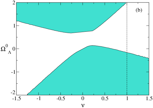
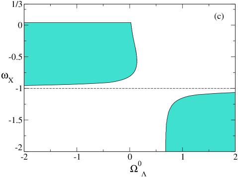
Figure 3: The projections of the $3D$-dimensional physical region of Fig. 2 onto the three planes: (a) $\Omega_{\Lambda}^{0}=const.$, (b) $\omega_{X}=const.$ and (c) $\nu=const.$

    

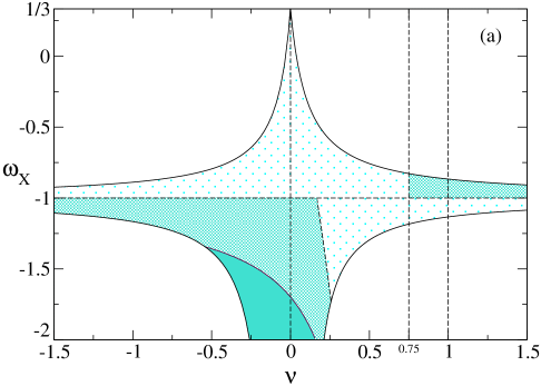
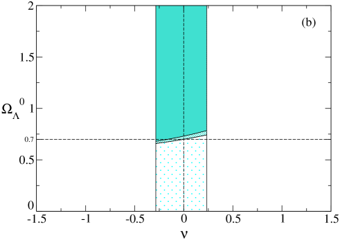
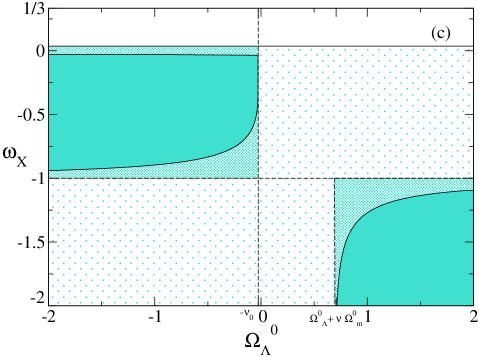
Figure 4: Different slices of the $3D$ volume representing the physical region, see Fig. 2. The dotted areas fulfill the nucleosynthesis condition. The shaded regions satisfy both the nucleosynthesis and stopping conditions. If we further require the condition (102) on the ratio $r=\rho_{D}/\rho_{m}$, we are left with the darkest shaded region. Slices shown in the figure: (a) Slice $\Omega^{0}_{\Lambda}=0.75$; (b) Slice $\omega_{X}=-1.85$; (c) Slice $\nu=-\nu_{0}$, where $\nu_{0}$ is defined in (22).

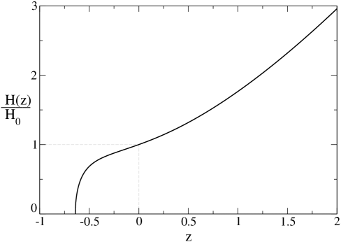
Figure 5: The Hubble function $H=H(z)$ for the values of the parameters: $\omega_{X}=-1.85,\,\Omega_{\Lambda}^{0}=0.75,\nu=-\nu_{0}$. This situation illustrates an example of Scenario VII (see Section 5). Condition (87) is satisfied and hence there is a stopping point in the future where $H$ vanishes and the expansion of the Universe stops.

The “physical region” is defined to be the subregion of the parameter space $(\ref{parameterspace2})$ satisfying these three conditions at the same time. It is illustrated in the $3D$-plot in Fig. 2. In Fig. 3 we can see the projection of the full $3D$ physical region onto three orthogonal planes $\Omega_{\Lambda}^{0}=const.$, $\omega_{X}=const.$ and $\nu=const.$ situated outside this region. It is also convenient to show cross-sections of the physical region, i.e. slices of the relevant volume for fixed values of the other parameters, just to check that the physical region is not just formed by a closed $2D$-surface, but rather by a $3D$-volume contained in the space (100). In Fig. 4 we show three slices $\Omega_{\Lambda}^{0}=const.$, $\omega_{X}=const.$ and $\nu=const.$ for particular values of these parameters that illustrate this feature. We note that in Fig. 3 we have allowed for $\omega_{X}$ to be slightly out in the range (51), only for completeness. In fact the region that does not satisfy condition (51) is seen to become narrower the larger becomes $\omega_{X}$, and therefore it is rather restricted.

7.2 Expansion rate and effective EOS

In Fig. 5 we show the expansion rate $H=H(z)$ of the $\Lambda$XCDM model as a function of the redshift for given values of the parameters: $\omega_{X}=-1.85,\,\Omega_{\Lambda}^{0}=+0.75,\,\nu=-\nu_{0}$, where $\nu_{0}$ is defined in (22). This selection of parameters corresponds to scenario VII in Section 5. Since Eq. (87) is fulfilled, there must be a stopping point ahead in time, which is indeed confirmed in Fig. 5 where we see that $H$ vanishes at some point in the future. As discussed in Section 5, the cause for the stopping in this case is actually attributed to the negative energy of the cosmon in the future (i.e. to the presence of “Phantom Matter” rather than to the effect of a negative cosmological term). The presence of a stopping point implies the existence of a maximum for the ratio between DE and matter densities, and this fact provides a natural explanation for the coincidence problem. In the present case the maximum exists because Eq. (88) is satisfied. Notice that the choice of parameters used in Fig. 5 has the attractive property that the value of $\Omega_{\Lambda}^{0}$ is very close to the current one in the standard $\Lambda$CDM model. However, it should be remembered that in all numerical examples discussed in this section we have fixed $\Omega_{D}^{0}$ as in (99). This means that in the particular numerical example illustrated in Fig. 5, the value of the cosmon density at present is rather small and negative: $\Omega_{X}^{0}=-0.05$.

    

    

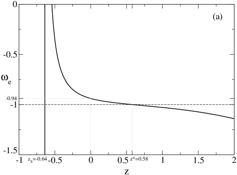
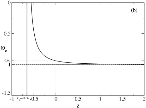
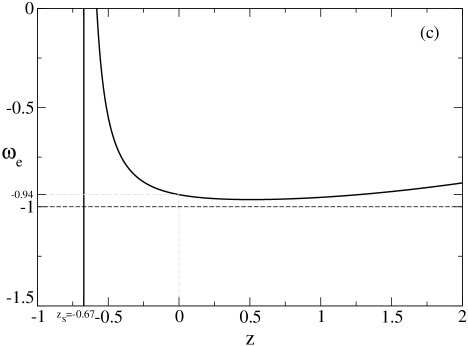
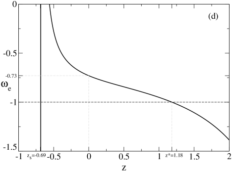
Figure 6: The effective EOS parameter of the $\Lambda$XCDM model, $\omega_{e}$ –defined in Eq. (7) –, as a function of the cosmological redshift, for different scenarios: (a) $\omega_{X}=-1.85,\,\Omega_{\Lambda}^{0}=0.75,\,\nu=-\nu_{0}$; (b) As in (a) but for $\nu=0$; (c) As in (a), but for $\nu=+\nu_{0}$; (d) $\omega_{X}=-0.93,\Omega_{\Lambda}^{0}=-2,\,\nu=+0.96$.

Very important for the future program of cosmological experiments [7, 8, 9] is the issue of the equation of state (EOS) analysis of the dark energy from the observational data. In the standard description of the DE, it is assumed that the DE consists of a self-conserved entity, or various entities of the same kind which produce a conserved total DE. As a particular case we have the standard $\Lambda$CDM model, where the DE is just the constant $\Lambda$. But we can also have simple quintessence models, with a single scalar field or multicomponent scalar fields [19, 27]. In the latter case one of the fields can be a (standard) phantom (cf. Fig. 1) and this has been proposed as a mechanism to explain the crossing of the cosmological constant divide [15]. In practice the experimental EOS

$$p_{D}=\omega_{\rm exp}\,\rho_{D}\,,$$ (103)

has to be determined by observations. This equation will be confronted with the theoretical predictions of any given model. For the theoretical analysis it is convenient to consider the general notion of effective EOS of the DE [36], namely the EOS that describes dark energy as if it would be a single self-conserved entity without interaction with matter . We write it as

$$p_{D}=\omega_{e}(z)\,\rho_{D},$$ (104)

where $\omega_{e}=\omega_{e}(z)$ is the theoretical EOS parameter or function in the effective DE picture, which is the one that should be compared with $\omega_{\rm exp}$ in (103). In the original model the DE could actually be a mixture of entities of very different kind, as indicated in (1). This is indeed the case for the $\Lambda$XCDM model where we have a non-barotropic mixture of cosmon and running cosmological constant. From the explicit solution of the model obtained in Section 3 we can study the numerical behavior of the effective EOS of the $\Lambda$XCDM model, see Eq. (7).

Before displaying our EOS results, we recall that the most recent WMAP data, in combination with large-scale structure and supernovae data, lead to the following interval of values for the EOS parameter [5]:

$$\omega_{\rm exp}=-1.06^{+0.13}_{-0.08}\,.$$ (105)

This result is quite stringent, and it does not depend on the assumption that the Universe is flat. However, it does depend on the assumption that the EOS parameter does not evolve with time or redshift. In this sense it is not directly applicable to the effective EOS of the $\Lambda$XCDM model. In general the experimental EOS parameter $\omega_{\rm exp}$ need not be a constant, and one expects it to be a function of the redshift, $\omega_{\rm exp}=\omega_{\rm exp}(z)$. Since this function is unknown, one usually assumes that it can be parametrized as a polynomial of $z$ of given order. This is, however, inconvenient to fit cosmological data at high redshifts; say, data from the CMB. And for this reason other parametrizations have been proposed and tested in the literature [11, 12, 13]. As an example, consider the following one [13],

$$\omega_{e}(z)=\omega_{0}+\omega^{\prime}_{0}\,\frac{z}{(1+z)^{p}}\,,\ \ \ (p=1,2)\,,$$ (106)

where $\omega^{\prime}_{0}=(d\omega_{e}/dz)_{z=0}$. The last parameter contemplates the possibility of a residual evolution of the DE even if $\omega_{0}=-1$. Notice that the asymptotic behavior of $\omega_{e}(z)$ in this parametrization is tamed: for $p=1$ one has $\omega_{e}(+\infty)=\omega_{0}+\omega^{\prime}_{0}$, and for $p=2$, $\omega_{e}(+\infty)=\omega_{0}$. This kind of parametrizations can be useful for a simplified treatment of the data. However, in general one should not be misled by them. The underlying dark energy EOS can be more complicated and may not adapt at all to a given parametrization. In this respect it should be kept in mind that there is also the possibility that the experimental EOS (103) is mimicked by other forms of DE that look as dynamical scalar fields without being really so. This possibility has been demonstrated in concrete examples in [37] and further generalized in [38]. In particular, in the analysis of [37] it is shown that the “effective EOS of a running cosmological model” can be analytically rather complicated; it does not adapt to the form (106) and nevertheless it provides a good qualitative description of the experimentally fitted EOS from the data [11]. In the following we will show, with specific numerical examples, that the effective EOS of the $\Lambda$XCDM model may account for the observed behavior of the DE in the redshift range relevant to supernovae experiments. In Section 7.4 we will show that even the asymptotic behavior of the $\Lambda$XCDM model at very high redshifts (relevant to the CMB analysis) completely eludes the class of models covered by simple parametrizations like (106). These parametrizations are, therefore, not model-independent, and the fits to the dark energy EOS derived from them should be handled with care and due limitation.

In Fig. 6 we plot $\omega_{e}=\omega_{e}(z)$ for the $\Lambda$XCDM model as a function of $z$ for some particular choices of the basic set of parameters (100) and within the typical accessible supernovae range [7]. On comparing these results with the experimental fit (105) we should stress again that the latter is only valid for a strictly constant EOS parameter. Even so, scenarios (a)-(c) of Fig. 6 satisfy this bound already at $1\,\sigma$. Scenario (d) satisfies it only at $\sim 2.5\sigma$, but here $\omega_{e}$ varies substantially with $z$.

All the plots in Fig. 6 exhibit a discontinuity at a certain point $z_{0}$ in the future, before reaching the stopping point $z_{s}$. A magnified view of this discontinuity for the case of Fig. 6a can be appreciated in Fig. 7. The discontinuity occurs when $\omega_{e}$ changes sign at a point $z_{0}$ where $\rho_{D}(z_{0})=0$. At this point $\omega_{e}(z_{0})$ becomes undefined, see Eq. (7). In a neighborhood $z_{0}^{\pm}=z_{0}\pm\varepsilon$ of the point $z_{0}$ we have $\omega_{e}(z_{0}^{\pm})=\pm\infty$ for $\varepsilon\rightarrow 0$. The singularity is not a real one, because all density functions remain finite at that point, so its existence only reminds us that the description in terms of the EOS parameter is inadequate near that point.

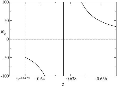
Figure 7: Detail of the discontinuity of the EOS function $\omega_{e}=\omega_{e}(z)$ at a point $z_{0}\lesssim-0.638$ in the future, corresponding to case (a) of Fig. 6. At this point $\rho_{D}(z_{0})=0$.

Looking at Fig. 6 we can see diverse scenarios. For example, in Fig. 6a we have a concrete example of the scenario VII (with $\nu<0$) defined in Section 5, the same one used in Fig. 5, namely $\omega_{X}=-1.85,\Omega_{\Lambda}^{0}=0.75,\nu=-\nu_{0}$. It corresponds to have $\Omega_{\Lambda}^{0}$ very near the standard $\Lambda$CDM value with the $\nu$ parameter fixed at the canonical value (22). At the same time the cosmon field, $X$, is phantom-like and it behaves as Phantom Matter in the future. We can also appreciate a mild transition of $\omega_{e}$ from phantom to quintessence behaviour at some point $z^{*}$ near past. This is the kind of possible transition we have foreseen analytically for the $\Lambda$XCDM model in Section 6. We can check that the crossing condition (i) in Eq. (95) is satisfied. If the transition is sufficiently mild and the average of $\omega_{e}$ around the transition point $z^{*}$ is close to $-1$ (as it is indeed the case here) it cannot be excluded by the present data. Notice that the phantom regime starts to be significant only for $z>1.5$ in this case. At the moment we do not have enough statistics on this region, and it is not obvious that we will ever have, at least using supernovae data alone. Recall that SNAP [7] is scheduled to possibly reach up to $z=1.7$, with a very meager statistics foreseen around this high redhshift end. In this sense, a mild phantom behavior around that distant regions will be difficult to exclude; in particular, a kind of smooth transition of the type Phantom $\rightarrow$ Quintessence (for increasing $z$) will always be a possibility to keep in mind. Notice that in all cases shown in Fig. 6 the value of $\omega_{e}(z)$ at $z=0$ is very close to $-1$, namely $\omega_{e}(z)=-0.94$ in the first three cases, and $\omega_{e}(z)=-0.73$ in the last one. As we have said, these values are sufficiently close to $-1$ to be acceptable in the light of the recent data and the priors used to fit it.

In Fig. 6b we display a situation corresponding to $\nu=0$. This is an example of scenario II in Section 5. In this case the cosmological term $\Lambda$ remains strictly constant and the stopping of the Universe is due to the super-deceleration produced by the cosmon (mainly in the future time stretch). Again $\Omega_{X}^{0}<0$, but here the cosmon behaves as Phantom Matter for the entire span of the Universe lifetime. For $\nu=0$, we can see that in the past $\omega_{e}$ approaches fast to $-1$ asymptotically. The reason for this can be seen e.g. in Eq. (5) – and more generally from (6) – which shows that in the asymptotic past the cosmon density $\Omega_{X}(z)$ is proportional to $\nu$. Figures  6c,d display other interesting situations. They constitute examples of scenarios VII and IV respectively (both with $\nu>0$). In particular, in Fig. 6c the EOS parameter approaches $\omega_{e}=-1$ for a long stretch of the accessible redshift range by SNAP, and therefore it mimics a constant cosmological term. This case is different from the one in Fig. 6b, where $\Lambda$ is strictly constant but the DE is not; here the $\Lambda$XCDM model behaves as the standard $\Lambda$CDM model for sufficiently large redshift. Finally, in 6d we have a situation where the cosmon is quintessence-like ($\omega_{X}>-1$) and nevertheless the effective behavior of the total DE displays a transition from phantom to quintessence regime. Again we can check that the crossing condition (i) in Eq. (95) is satisfied.

     .

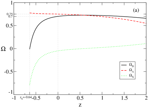
Figure 8: The total and individual DE densities, $\Omega_{D}=\Omega_{D}(z)$, $\Omega_{\Lambda}=\Omega_{\Lambda}(z)$ and $\Omega_{X}=\Omega_{X}(z)$ for two different situations where the cosmon barotropic index is of phantom-type ($\omega_{X}<-1$) and of quintessence-type ($\omega_{X}\gtrsim-1$) respectively: (a) $\omega_{X}=-1.85,\,\Omega_{\Lambda}^{0}=0.75,\,\nu=-\nu_{0}$; (b) $\omega_{X}=-0.93,\,\Omega_{\Lambda}^{0}=-2,\,\nu=0.96$. The two examples correspond to cases (a) and (d) of Fig. 6.

7.3 Evolution of the DE density and its components

The behavior of the effective EOS parameter $\omega_{e}$ is related to that of the DE densities in Eq. (7). The interaction of the cosmon and the cosmological term produces a curious effect; namely, the evolution of the cosmon density, $\Omega_{X}$, does not follow the expectations that we would usually have for a fluid $X$ carrying a value $\omega_{X}>-1$ or $\omega_{X}<-1$ of its barotropic index. For a better understanding of the situation we have plotted in Fig. 8a,b the total density $\Omega_{D}(z)$, as well as the two individual components $\Omega_{\Lambda}(z)$ and $\Omega_{X}(z)$, for two particular cases: one with the same parameters as in Fig. 6a (in which the cosmon has $\omega_{X}<-1$ as if it were a standard phantom field), and the other for the same parameters as in Fig. 6d (where the cosmon has $\omega_{X}>-1$ as if it were a conventional quintessence field). We can appreciate from these figures the sign changes of the various DE densities with the Universe evolution. In particular, in Fig. 8a the cosmon density appears to be $\Omega_{X}>0$ in the intermediate past but it starts behaving as Phantom Matter ($\Omega_{X}<0$, cf. Fig. 1) near our recent past and also at present, and this trend is enhanced in the future. In contrast, for the case of Fig. 8b the $X$ density changes fast from $\Omega_{X}<0$ to $\Omega_{X}>0$ at some point in the past (and stays so all the way into the future). Now, due to its interaction with the variable $\Lambda$, the quintessence-type cosmon ($\omega_{X}\gtrsim-1$) of Fig. 8b does not decay with the expansion; it actually grows fast as if it were a true phantom! The overall result is that, thanks to the concomitant depletion of the $\Lambda$ density into the negative energy region (very evident in the figure), there is a net deceleration of the expansion and a final arrival at the stopping point. Notice that, in contrast to the hectic evolution of the two component $\Omega_{\Lambda}(z)$ and $\Omega_{X}(z)$, the total DE density $\Omega_{D}(z)$ evolves quite slowly. A different behavior is observed for the phantom-type cosmon ($\omega_{X}<-1$) in Fig. 8a. In this case, rather than increasing rapidly with the expansion, the cosmon density actually decreases slowly (it actually behaves for a while as standard quintessence) and then at some future point near our time it “transmutes” into Phantom Matter and causes a fast deceleration of the expansion, with an eventual stopping of the Universe. In this case, the total DE density $\Omega_{D}(z)$ again evolves very mildly. The behaviors in Fig. 8a,b are an immediate consequence of Eq. (18), which implies that the $\Lambda$XCDM model effectively behaves as quintessence if and only if $\alpha_{X}$ and $\Omega_{X}$ have the same signs, as it is indeed the case here.

Recall that in all cases considered in our numerical analysis the total DE density is normalized to (99) at $z=0$, as can be checked in the examples presented in Fig. 8. In this figure it is remarkable the stability of $\Omega_{D}(z)$ in the entire range relevant to SNAP experiments [7] both for small $\nu$ (Fig. 8a) and large $\nu$ (Fig. 8b). This is due to the nucleosynthesis constraint and to the small values of the cosmon parameters $\alpha_{X}$ and/or $\Omega_{X}^{0}$ in these examples. To see this, let us first expand the total DE density (36) in the small parameter $\epsilon$ in first order:

$$\Omega_{D}(z) \simeq\frac{\Omega_{\Lambda}^{0}-\nu}{1-\nu}-\frac{\epsilon\,\Omega_{m}^{0}}{\omega_{m}-\omega_{X}}\,(1+z)^{\alpha_{m}}+\left\{\frac{1-\Omega_{\Lambda}^{0}}{1-\nu}-\Omega_{m}^{0}\right.$$ (107)

$$\left.+\frac{\epsilon\,\Omega_{m}^{0}}{\omega_{m}-\omega_{X}}-3\,\epsilon\,\left[\,\frac{1-\Omega_{\Lambda}^{0}}{1-\nu}-\Omega_{m}^{0}\right]\,\ln(1+z)\right\}\,(1+z)^{\alpha_{X}}\,.$$

Next, expanding this equation linearly in $z$, the $\nu$-dependence cancels and we find a very simple result:

$$\Omega_{D}(z)\simeq\Omega_{D}^{0}+\alpha_{X}\,\Omega_{X}^{0}\,z\,.$$ (108)

This expression coincides with the expansion, up to the linear term in $z$, of the function (76). The latter is the DE density for the $\nu=0$ case – see scenarios I and II of Section 5. Therefore, we arrive at the following remarkable result: due to the nucleosynthesis constraint, the DE density of the $\Lambda$XCDM model behaves always (i.e. for any $\nu$) as in the $\nu=0$ case in the region of small $z<1$ (up to terms of order $\epsilon^{2}$). As a consequence the evolution of $\Omega_{D}$ with the redshift will be mild in this region provided $\alpha_{X}$ is small or $\Omega_{X}^{0}$ is small, or both. Since $\nu$ has dropped in the linear approximation (108), this result is independent of $\nu$. Therefore, $\nu$ can be large (meaning $|\nu|\sim 1$) and still have a sufficiently “flat” evolution of $\Omega_{D}(z)$ for $z\lesssim 1$ . We can appreciate particularly well this feature in the situation depicted in Fig. 8a, where the cosmon energy density is very low (in absolute value) both in the intermediate past and also near the present. Thus both the total DE density $\Omega_{D}(z)$ and the cosmological term density, $\Omega_{\Lambda}(z)$, remain virtually constant for a long period in our past and in our future - see the plateau $\Omega_{D}\simeq const.$ in Fig. 8a. Although in this example the cosmon density, $\Omega_{X}$, remains very small in our past and around our present ( $|\Omega_{X}|\ll\Omega_{\Lambda}$), in the future $\Omega_{X}$ dives deeply into the Phantom Matter region and eventually controls the fate of the Universe’s evolution. So the cosmon density, which is negligible for the redshift interval relevant to SNAP measurements, does become important in the future and is finally responsible for the stopping of the Universe. Similarly, in Fig. 8b we have a large value of $\nu$ around $1$ and $\Omega_{D}$ stays also rather flat. In this case the flat behavior is due to $\alpha_{X}\ll 1$. In both situations represented in Fig. 8 the $\Lambda$XCDM model mimics to a large extent the standard $\Lambda$CDM model.

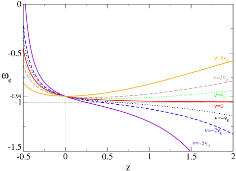
Figure 9: Comparison of the effective EOS parameter of the $\Lambda$XCDM model, $\omega_{e}$, for fixed values of $\omega_{X}$ and $\Omega_{\Lambda}^{0}$ ($\omega_{X}=-1.85$, $\Omega_{\Lambda}^{0}=0.75$, as in Fig. 6a) and different values of $\nu$ in units of $\nu_{0}$, Eq. (22). All curves give $\omega_{e}(0)=-0.94$ at the present time.

Recall from Section 3 that in the limit of vanishingly small $\nu$ and $\Omega_{X}^{0}$ the $\Lambda$XCDM model boils down exactly to the standard $\Lambda$CDM model. The result proven above, however, tells us something new: namely, if $z$ is not too large ($z\lesssim 1$, still within most of the SNAP range), the coincidence between the two models can still be maintained under appropriate circumstances (small $\alpha_{X}$ and/or $\Omega_{X}^{0}$), even if $\nu\neq 0$, by virtue of the nucleosynthesis constraint on the parameter $\epsilon$. Therefore, the following question is now in order. Under these circumstances, how can one possibly differentiate between the two models in a practical way (e.g. using the future SNAP experiments)? The answer is straightforwardly simple: by looking closely at the EOS behavior which, contrary to the DE density, can be very sensitive to the value of $\nu$! In fact, the size and sign of $\nu$ can play a key role to modulate the quintessence/phantom behavior effectively developed by the $\Lambda$XCDM model at moderate values of $z$ accessible to experiment. The EOS behavior has been displayed in Fig. 6, but the $\nu$-sensitivity of this behavior can be much better appreciated in the comparative set of EOS curves shown in Fig. 9, which have been performed for various values of $\nu$ (with both signs) and for fixed values of the other parameters. For a cosmon of the “$\omega_{X}<-1$ type”, we can see that a positive value of $\nu$ helps to lift the EOS curve into the quintessence region and, therefore, it helps to resemble more to some recent EOS analyses of the data, which seem to favor the existence of a mild quintessence-regime in our recent past  [11, 13]. For $\nu<0$ (and small), instead, the curve gently crosses the cosmological constant divide and plunges slowly into the phantom regime at higher and higher $z$. For a “$\omega_{X}>-1$ type” cosmon, instead, these features are opposite (cf. Fig. 6d). Finally, for $\nu=0$ the curve stabilizes very rapidly (at increasingly high redshifts) along the flat line $\omega_{e}=-1$ and the $\Lambda$XCDM model looks in this case essentially as the standard $\Lambda$CDM both from the point of view of EOS behavior and constancy of the DE density. This is because $\alpha_{X}<0$ in Fig. 9, meaning that $\Omega_{D}(z)\rightarrow\Omega_{\Lambda}^{0}$ for $z$ sufficiently deep in the past (see next section). But even in this case the effective EOS starts changing softly at some point near our past, and then steadily fast in the future, until it breaks into a singular (but spurious) behavior at a point $z_{0}$ where $\rho_{D}(z_{0})=0$ and $\omega_{e}(z_{0})$ becomes undefined.

7.4 Asymptotic regime of the EOS in the past

Let us study the behavior of the effective EOS in the asymptotic past, $z\gg 1$. This will help to substantiate the behavior of the numerical examples considered above and reveal additional features. From Eq. (6) we find

$$\Omega_{X}(z\gg 1)=\left\{\begin{array}[]{ll}-b\,\Omega_{X}^{0}\,(1+z)^{\alpha_{m}},&\,\,\,\,\,\,{\text{for}}\,\,\nu\neq 0\\ &\\ \hskip 28.45274pt0&\,\,\,\,\,\,{\text{for}}\,\,\nu=0,\ \ \alpha_{X}<0\\ &\\ \hskip 14.22636pt\Omega_{X}^{0}\,(1+z)^{\alpha_{X}}&\,\,\,\,\,\,{\text{for}}\,\,\nu=0,\ \ \alpha_{X}>0\,,\end{array}\right.$$ (109)

where $b$ is given by (93). Consider next the exact expression for $\Omega_{D}(z)$, given in (36). The asymptotic behavior of this expression in the past is

$$\Omega_{D}(z\gg 1)=\left\{\begin{array}[]{ll}-\frac{\epsilon}{\omega_{m}-\omega_{X}+\epsilon}\,\Omega_{m}^{0}\,(1+z)^{\alpha_{m}},&\,\,\,\,\,\,{\text{for}}\,\,\nu\neq 0\\ &\\ \hskip 28.45274pt\Omega_{\Lambda}^{0}&\,\,\,\,\,\,{\text{for}}\,\,\nu=0,\ \ \alpha_{X}<0\\ &\\ \hskip 14.22636pt\Omega_{X}^{0}\,(1+z)^{\alpha_{X}}&\,\,\,\,\,\,{\text{for}}\,\,\nu=0,\ \ \alpha_{X}>0\,.\end{array}\right.$$ (110)

For completeness let us also quote

$$\Omega_{\Lambda}(z\gg 1)=\left\{\begin{array}[]{ll}\frac{\nu\,(\omega_{m}-\omega_{X})}{\omega_{m}-\omega_{X}+\epsilon}\,\Omega_{m}^{0}\,(1+z)^{\alpha_{m}}\simeq\nu\,\Omega_{m}^{0}\,(1+z)^{\alpha_{m}}\,,&\,\,\,\,\,\,{\text{for}}\,\,\nu\neq 0\\ &\\ \hskip 28.45274pt\Omega_{\Lambda}^{0}&\,\,\,\,\,\,{\text{for}}\,\,\nu=0\,.\end{array}\right.$$ (111)

We can indeed check out the predicted trends for the various DE densities on inspection of Fig. 8. Substituting equations (109) and (110) into (7), and using (93), we find the corresponding asymptotic behavior of the effective EOS parameter in the past:

$$\omega_{e}(z\gg 1)=-1+(1+\omega_{X})\,\frac{\Omega_{X}(z\gg 1)}{\Omega_{D}(z\gg 1)}=\left\{\begin{array}[]{ll}\omega_{m}&\,\,\,\,\,\,{\text{for}}\,\,\nu\neq 0\\ &\\ -1&\,\,\,\,\,\,{\text{for}}\,\,\nu=0,\ \ \alpha_{X}<0\\ &\\ \omega_{X}&\,\,\,\,\,\,{\text{for}}\,\,\nu=0,\ \ \alpha_{X}>0\,.\end{array}\right.$$ (112)

On the one hand the asymptotic results for $\omega_{e}$ in the case $\nu=0$ were easily foreseeable from the structure of Eq. (7), because in this case (that is, in the absence of interaction between the cosmon and $\Lambda$) the growing and decreasing properties of the cosmon density strictly follow its canonical quintessence or phantom character in each case. In other words, for $\nu=0$ a cosmon carrying a phantom-type or quintessence-type $\omega_{X}$-label does properly behave as a standard phantom or quintessence, respectively. (Not so, however, when $\nu\neq 0$, as we have seen!) On the other hand the asymptotic result for $\omega_{e}$ in the case $\nu\neq 0$ came a bit of a surprise. It implies that at very high redshift the effective EOS of the DE in the $\Lambda$XCDM model coincides with that of matter-radiation. This does not cause any harm to nucleosynthesis, for as shown by Eq. (110) the asymptotic DE density remains bounded by the constraint (50). This prediction of the $\Lambda$XCDM opens the possibility that the CMB data could actually be blind to the EOS analysis of the DE. Indeed, as we have mentioned above the CMB fits usually assume parametrizations of the form (106) and the like. In general one replaces Eq. (16) into the expansion rate (35) to get (for $\Omega_{K}^{0}=0$)

$$H^{2}(z)=H_{0}^{2}\,\left[\Omega_{m}^{0}\,(1+z)^{\alpha_{m}}+\,\Omega_{D}^{0}\,\exp\left\{3\,\int_{0}^{z}\,dz^{\prime}\frac{1+\omega_{e}(z^{\prime})}{1+z^{\prime}}\right\}\right]\,.$$ (113)

Whatever it be the “well-behaved” parametrization assumed for $\omega_{e}$ at high redshift, if it leads to powers of $1+z$ in the function $H=H(z)$, the fact that $z\simeq 1100$ for the CMB analysis will unavoidably provide a fit of $\omega_{e}$ very close to $\,-1$. For example, in the case of Eq. (106) for $p=1$, we find

$$H^{2}(z)=H_{0}^{2}\,\left\{\Omega_{m}^{0}\,(1+z)^{\alpha_{m}}+\Omega_{D}^{0}\,(1+z)^{3(1+\omega_{0}+\omega^{\prime}_{0})}\,\exp\left[-3\,\omega^{\prime}_{0}\,\frac{z}{1+z}\right]\right\}\,.$$ (114)

This equation reduces to the standard $\Lambda$CDM one for $\omega_{0}=-1,\omega^{\prime}_{0}=0$, as expected. At the same time it is clear that fitting data at very high redshift (e.g. CMB data) with (114) will naturally convey $\omega_{e}\simeq-1$ – if one wants to match at the same time the LSS and supernovae data both suggesting that $\Omega_{D}^{0}$ is of the same order as $\Omega_{M}^{0}$. Therefore, finding $\omega_{e}\simeq-1$ from (114) can be an intrinsic bias or artifact of the parametrization itself.

In contrast, if the underlying theory of the DE would exhibit a behavior of the $\Lambda$XCDM type (112), the CMB data could not be sensitive to the EOS parameter in its conventional form and the observations should be interpreted in a different way. Namely, the canonical result $\omega_{e}\simeq-1$ could only be derived for “small” or intermediate redshift of the order of the distant Type Ia supernovae, where the $\Lambda$XCDM model can resemble to a large extent the standard $\Lambda$CDM. In the new scenario the result (112) for $\nu\neq 0$ could still be detected by observing a “mass renormalization” effect of the cosmological parameter $\Omega_{m}^{0}$ when comparing the two sets of results for small and high redshifts, i.e. when comparing supernovae data fits with CMB fits. Indeed, substituting (110) in (35) one gets, at very high redshift (neglecting the curvature term)  :

$$H^{2}(z)\simeq H_{0}^{2}\,\hat{\Omega}_{m}^{0}\,(1+z)^{\alpha_{m}}$$ (115)

where the “renormalized” cosmological mass parameter is:

$$\hat{\Omega}_{m}^{0}=\Omega_{m}^{0}\,\left(1-\frac{\epsilon}{\omega_{m}-\omega_{X}+\epsilon}\right)\,.$$ (116)

The relative difference $|\hat{\Omega}_{m}^{0}-\Omega_{m}^{0}|/\Omega_{m}^{0}$ between the two determinations of $\Omega_{m}^{0}$ is just given by the nucleosynthesis constraint on the parameter $r=\rho_{D}/\rho_{m}$, see Eq. (50). Thus it could lead to a measurable $\sim 10\%$ effect that would provide a distinctive signature of the model. There is nothing odd in the DE behaving this way; the DE density (110) is still there all the time even though the conventional EOS analysis could miss it. In this case one must resort to a different interpretation which may lead to its determination.

Let us also note that since $\omega_{m}\geqslant 0$, then in those ($\nu\neq 0$) cases where there is a crossing point $z^{*}$ from phantom into quintessence regime there must necessarily be a point in the past where $\rho_{D}$ becomes zero and changes sign. This produces another spurious singularity in the function $\omega_{e}$. (Recall from Section 6 that we cannot have more than one crossing point $z^{*}$.) In this case the evolution of $\omega_{e}$ from the asymptotic regime $\omega_{e}(z\gg 1)\simeq\omega_{m}>0$ up to the singularity, is such that $\omega_{e}$ stays above $-1$. After the fake singularity is crossed towards $z=z^{*}$, the value of $\omega_{e}$ emerging from it is smaller than $-1$, and remains so until reaching the crossing point $z^{*}$ where again $\omega_{e}$ becomes larger than $-1$.

For experiments like SNAP [7] the relevant redshift range (a window of small and moderate redshifts up to $z=1.7$) is far away from the asymptotic regime. Here the rich panoply of behaviors exhibited by the effective EOS of the $\Lambda$XCDM model is very evident in e.g. Figs. 6 and 9. Some of these traits should in principle be observable in these experiments and should be the most conspicuous ones. However, as repeatedly emphasized, the effective EOS behavior of the $\Lambda$XCDM model in that redshift range can approximate to a great extent that of the $\Lambda$CDM model – either because it is very close to $\omega_{e}=-1$ or because there is a gentle transition (from phantom-like behavior into quintessence one) while keeping an average value $\omega_{e}=-1$.

    

    

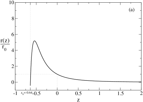
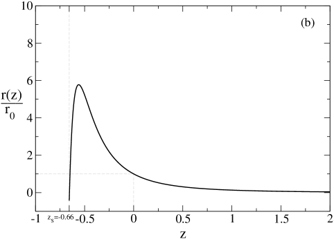
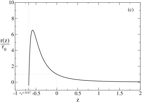
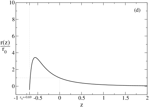
Figure 10: The ratio $r=\rho_{D}/\rho_{m}$, Eq. (41), as a function of the redshift (in units of the current ratio, $r_{0}$), for the following values of the parameters: (a) $\omega_{X}=-1.85,\Omega_{\Lambda}^{0}=0.75,\nu=-\nu_{0}$;(b) As before, but for $\nu=0$; (c) The same, but for $\nu=+\nu_{0}$; (d) $\omega_{X}=-0.93,\Omega_{\Lambda}^{0}=-2,\nu=0.96$.

7.5 Evolution of the ratio $r=\rho_{D}/\rho_{m}$ and the cosmological coincidence problem

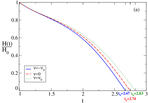
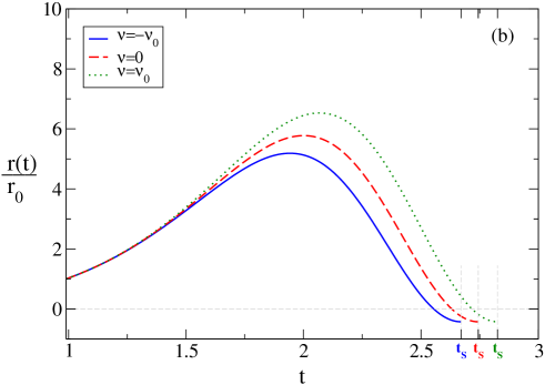
Figure 12: (a) The expansion rate of the $\Lambda$XCDM model in terms of the cosmic time, $H=H(t)$, for the same parameter choices as in Fig. 10a,b,c; (b) The ratio $r=\rho_{D}/\rho_{m}$, in units of its present value $r_{0}$, as a function of the cosmic time for the same scenarios as in (a). In both cases the cosmic time is measured in Hubble time units $H_{0}^{-1}$. The present time lies at $t_{0}=13.7\,Gyr$, i.e. $\sim 0.98\,H_{0}^{-1}$

In Fig. 10 we display the ratio $r$, Eq. (41), in units of the current ratio ($r_{0}\simeq 7/3$) as a function of the cosmological redshift variable, for various values of the parameters. All the plots in Figs. 10 and 12 exhibit a maximum below 10. However, let us clarify that there are regions of parameter space where the maxima can be much higher, but in any case finite. Having a model where the ratio $r=\rho_{D}/\rho_{m}$ is bounded for the whole Universe lifetime provides a natural explanation for the cosmological coincidence problem. One may view the property $r_{0}\sim 1$ as a simple corroboration of the fact that we live at a cosmic time near the transition redshift $z_{t}$ where the Universe changed from decelerated expansion into an accelerated one. But this observation leaves the coincidence problem in the same place. For instance, in the standard $\Lambda$CDM model, once the redshift $z_{t}$ is trespassed by the evolution the ratio $r(z)$ starts to grow without end. So it is a kind of puzzling “coincidence” that we just happen to live so near the transition point $z_{t}$. This assertion should not be understood on anthropic grounds. When we say that it is a coincidence to “live near the transition point $z_{t}$” we mean that the probability to find a lapse of the Universe’s lifetime where $r(z)\simeq 1$ should be essentially zero for a Universe (like the standard $\Lambda$CDM) where this ratio is larger than any given number if we await enough time. In the $\Lambda$XCDM model, instead, the situation is quite different. If the Universe would still be populated by some form of intelligent life in the remote future, say $5-10$ billion years from now, and these beings would be curious enough to perform a new measurement of $r(z)$ at their time, they might learn that $r(z)$ is no longer $r_{0}$, as it is now, but maybe something like $2\,r_{0}$ or $5\,r_{0}$, or even back to $r_{0}$ at some later time (where the Universe would in this case be decelerating rather than accelerating). There would be no correlation between the value $r(z)\sim 1$ and the state of acceleration of the Universe, and they would not be compelled to conclude that they are living in a very peculiar spell of time. We can confirm this picture by looking at some numerical examples in Fig. 10 and 11. In particular, in Fig. 11 we demonstrate the dependence of the maximum on the value of $\nu$ for fixed values of the other parameters.

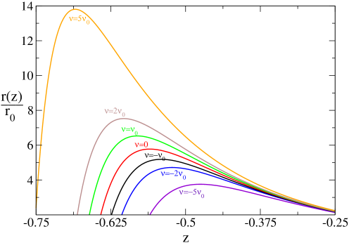
Figure 11: Comparison of the maximum of the ratio $r=\rho_{D}/\rho_{m}$ for $\omega_{X}=-1.85$, $\Omega_{\Lambda}^{0}=0.75$ (as in Fig. 10a) and different values of $\nu$.

For a more physical grasp of the situation, we have also solved numerically the $\Lambda$XCDM model in terms of the cosmic time variable $t$ (cf. Fig. 12). In this case it is not possible to provide analytic expressions such as (3) or (71) in terms of the $z$ and $\zeta$ variables respectively. We limit ourselves to provide the numerical result for the expansion rate $H=H(t)$ (Fig. 12a) and the ratio $r=r(t)$ (Fig. 12b) in units of the present ratio $r_{0}$ for the cases (a),(b) and (c) of Fig. 10. We can see that in terms of the cosmic time the distribution of the relevant events in the future (such as the reaching of the maximum and the arrival at the turning point) is not as sharp and abrupt as it was in terms of the redshift variable. Indeed, one can see that in terms of the cosmic time the maximum takes place far away in the future, typically at around $2$ Hubble times ($H_{0}^{-1}$) since the beginning of the expansion, i.e. roughly one Hubble time after our time, where $H_{0}^{-1}\simeq 14\,Gyr$ for $h_{0}=0.7$. The stopping point can typically lie at around $t_{s}\sim(2.5-3)\,H_{0}^{-1}$. To avoid cluttering, scenario (d) of Fig. 10 is not included in Fig. 12, but we have checked that it amounts to a lower maximum ($r<4$), and the stopping point lies at $t_{s}\gtrsim 3.5\,H_{0}^{-1}$.

From our detailed analysis of the ratio $r=\rho_{D}/\rho_{m}$ we may assert that the $\Lambda$XCDM model provides a possible solution (and in any case highly alleviates) the cosmological coincidence problem. At the very least it offers an alternative explanation to some other interesting proposals discussed in the literature [41, 42, 43, 55]. For example, in phantom dominated universes one may compute the fraction of the lifetime of the Universe where the ratio (43) stays within given bounds before the doomsday [43]. Recall that these universes are threatened and eventually killed by a final Big Rip, so that the idea is to compute the time interval between the start of acceleration and the time when the Universe is dismantled to its ultimate fundamental components, and compare it with the total lifetime. If the fraction is not very small, one may feel satisfied with this explanation. However, we can see that a purely phantom Universe is just a very particular case of $\Lambda$XCDM Universe, namely it corresponds to $\Lambda_{0}=\nu=0$ and $\alpha_{X}<0,\,\Omega_{X}^{0}>0$. In a general $\Lambda$XCDM Universe the range of possibilities is much larger, e.g. there can be a turning point rather than a Big Rip, the ratio (43) can stay bounded during the entire span of the Universe lifetime, and finally the matter is not destroyed.

Recall from the analytical discussion in Sections 4 and 5 that we have three critical points in the future: $z_{s}$ (stopping/turning point), $z_{0}$ (point where the total DE density vanishes and $\omega_{e}$ becomes singular), and $z_{\rm max}$ (point in the future where the ratio $r(z)$ attains its maximum). They are ordered as follows:

$$z_{s}<z_{0}<z_{\rm max}\,.$$ (117)

In correspondence we have the following values of the ratio (41):

$$r(z_{s})=-1<r(z_{0})=0<r(z_{\rm max})\lesssim 10\,.$$ (118)

At the same time we may compare the evolution undergone by $r(z)$ from the nucleosynthesis time through the present time till the maximum. We have exemplified typical situations in which

$$|r_{N}|\simeq 0.1<r_{0}\simeq 1<r(z_{\rm max})\lesssim 10\,.$$ (119)

Namely, the ratio of the DE density to the matter density undergoes a slow evolution within a few orders of magnitude. In this context it does not look bizarre that its present value is of order one. It should, however, be clear that the condition $\rho_{D}/\rho_{m}\sim 1$ is not guaranteed for any given point of the $\Lambda$XCDM parameter space. In this paper we have not addressed the computation of the probability distribution for the two energy levels $\rho_{D}$ and $\rho_{m}$ to be comparable at a particular time of the cosmic evolution. In the $\Lambda$XCDM model discussed here the complete solution, including the dynamics of the energy density levels at a particular time, depends deterministically on the set of values of the free parameters in Eq. (100). If we would discretize the parametric space, i.e. dividing it into small 3D elements, and then calculate the dynamics for every volume element, it would be possible to numerically construct the joint probability distribution for the matter and (composite) dark energy density levels at some fixed time. Since the volume of the parametric space is infinite, one would need to introduce additional constraints in order to select a finite volume of parametric space and make this calculation useful. Although an explicit construction of this distribution could indeed be performed after defining these constraints, our presentation actually provided an alternative procedure which should serve equally well our purposes; namely, we explicitly computed that part of the total parameter space which results in the wanted dynamics (that is to say, the ratio $r=\rho_{D}/\rho_{m}$ being bounded from above with the value of maximal $r$ within an order of magnitude from the present one) and showing that it is non-negligible. This is patent in Fig. 2, where the ”physical region” (viz. the one satisfying the aforementioned requirements) is exhibited. What we have found is that the dimensionality of the ”physical region” is the same as the dimensionality of the entire parametric space itself, in other words: the “physical region” is of non-zero measure in the space $(\Omega_{\Lambda}^{0},\omega_{X},\nu)$. Not only so, the fractional volume (referred to the volume of the region where the parameters stay within their “natural” values, see Fig. 2) is sizeable, as shown by the various projections onto the different planes displayed in Fig.  3-4. This proves that no additional fine-tunings are necessary to realize this scenario which is, in that sense, natural within the $\Lambda$XCDM models. This fact, combined with the nice features of the effective EOS of dark energy (described in Section 7.2) at the redshifts amenable to distant supernovae observations (and the compatibility with the nucleosynthesis bounds), further reinforces the $\Lambda$XCDM models as models with acceptable behavior of dark energy which at the same time provide an acceptable explanation (or substantial alleviation) of the coincidence problem.

  

7.6 Transition from deceleration to acceleration

A precise measurement of the transition redshift $z_{t}$ from deceleration into acceleration could also help to restrict the parameters of a given model. The value of $z_{t}$ is obtained theoretically by considering the change of sign of the deceleration parameter from $q(z)>0$ to $q(z)<0$, where

$$q(z)=-\frac{\ddot{a}\,a}{\dot{a}^{2}}=-\frac{\ddot{a}}{a\,H^{2}(z;\nu)}=\frac{1}{2}\,\left[(1+3\,\omega_{m})\,\tilde{\Omega}_{m}(z)+(1+3\,\omega_{e})\,\,\tilde{\Omega}_{D}(z)\right]\,.$$ (120)

The cosmological functions $\tilde{\Omega}_{D}(z)$ and $\tilde{\Omega}_{m}(z)$ are defined in (39). Since the the point $z_{t}$ is reached during the matter epoch, where $\omega_{m}=0,\ \omega_{e}<0$, we can define $z_{t}$ as the point that satisfies $q(z_{t})=0$, hence

$$\frac{\tilde{\Omega}_{D}(z_{t})}{\tilde{\Omega}_{m}(z_{t})}=\frac{1}{3\,|\omega_{e}|-1}\,.$$ (121)

In the standard $\Lambda$CDM model the corresponding relation reads ${\tilde{\Omega}_{D}(z_{t})}={\tilde{\Omega}_{m}(z_{t})}/2$, which is recovered from (121) after setting $\omega_{e}=-1$ and identifying $\Omega_{D}$ with $\Omega_{\Lambda}^{0}$. Equivalently, the deceleration parameter can be computed from the expansion rate $H(z)$ as follows,

$$q(z)\,=\,-1+\frac{1}{2}\,(1+z)\,\frac{1}{H^{2}(z)}\,\frac{dH^{2}(z)}{dz}\,,$$ (122)

and $z_{t}$ satisfies $q(z_{t})=0$. For the standard $\Lambda$CDM model and using the favorite values $\Omega_{M}^{0}=0.3$ and $\Omega_{\Lambda}^{0}=0.7$ of the cosmological parameters in the flat case, one obtains

$$z_{t}=-1+\sqrt[3]{2\,\frac{\Omega_{\Lambda}^{0}}{\Omega_{M}^{0}}}\simeq 0.67\,.$$ (123)

For the $\Lambda$XCDM model the expansion rate $H=H(z)$ is more complicated and is of course sensitive to the basic set of parameters (100) through the formula given in the first expression in Eq. (3). However, due to the relatively wide experimental margin obtained for $z_{t}$ (cf. Riess et al. in [2])

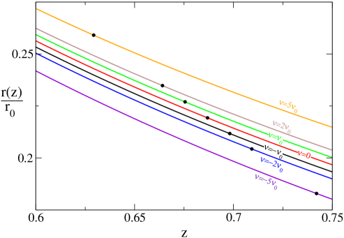
Figure 13: Comparison of the transition redshift $z_{t}$ (deceleration-acceleration) for $\omega_{X}=-1.85$, $\Omega_{\Lambda}^{0}=0.75$) and different values of $\nu$.

$$z_{t}^{\rm exp}=0.46\pm 0.13\,,$$ (124)

it is not possible at the moment to firmly discriminate which value of $\nu$ is preferred. Notice that the range (124) excludes the standard model value (123) by a bit more than one standard deviation, but this is not very significant for the moment. We expect that this situation will substantially ameliorate in the future. In the meanwhile from Fig. 13 we test the sensitivity of the transition redshift $z_{t}$ to the value of $\nu$ in the $\Lambda$XCDM. It seems to favor positive values of $\nu$. It is interesting to note that the $z_{t}$ sensitivity to $\nu$ is opposite in the $\Lambda$XCDM as compared to the pure running $\Lambda$ model of Ref. [23]. In the latter the values $\nu<0$ are favored (see particularly Fig. 4 of the second reference in  [23]). This is an example of how the observables can discriminate between two different realizations of a cosmological RG model. Both models, the $\Lambda$XCDM and the running $\Lambda$ model of [23] are based on a similar RG framework. However, in the latter matter is not self-conserved (there is exchange of energy between matter and the running $\Lambda$) whereas in the present model matter is self-conserved and the running $\Lambda$ can exchange energy only with the cosmon. Obviously, it will be necessary a comparison of several high precision observables (a task presumably feasible thanks to the next generation of observational experiments) before we can discriminate between the two kinds of RG cosmologies. Another observable that should help to discriminate between models is the EOS itself and the existence of a transition point $z^{*}$ where the model might effectively change from quintessence to phantom-like behavior or vice versa. For example, the RG model of [23] may have transitions from quintessence into phantom, as was shown in Ref. [37], whereas the $\Lambda$XCDM model can only have transitions of the opposite kind, or no transition whatsoever if stopping is required (cf. Section 6). Let us also add that the RG model of [23] does not have any clue, in contradistinction to the present $\Lambda$XCDM model, as to finding an explanation for the cosmological coincidence problem because the ratio (41) – which in that model just reads $\rho_{\Lambda}(z)/\rho_{M}(z)$ – is unbounded.

    

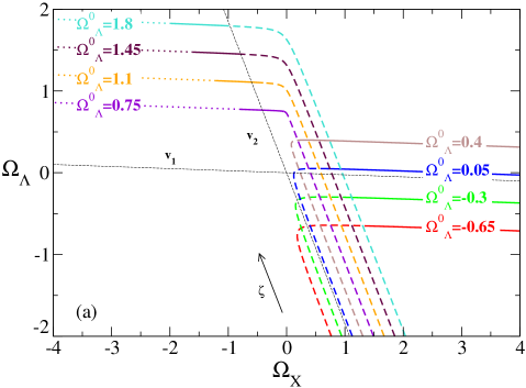
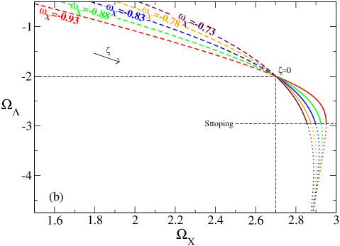
Figure 14: Phase trajectories of the autonomous system (5) in the $(\Omega_{\Lambda},\Omega_{X})$ plane. Dashed lines show the parts of the curves corresponding to positive redshifts (i.e. our past), full lines indicate the parts between the present moment and the stopping (if there is stopping) and dotted lines denote the inaccessible part of the trajectory after the stopping. (a) Example of scenario VII in Section 5 (saddle point case) corresponding to $\omega_{X}=-1.85$, $\nu=-\nu_{0}$. The eigenvector directions (69) are also marked. The various trajectories correspond to different choices of $\Omega_{\Lambda}^{0}$ indicated in the figure; (b) Example of scenario IV with a node determined by $(\nu,\Omega_{\Lambda}^{0})$; in the figure $\Omega_{\Lambda}^{0}=-2$, $\nu=0.96$. All trajectories are attracted towards the node (79), but they get stopped on the way to it. The point $\zeta=0$ corresponds to the present. The cosmic evolution is in the $\zeta>0$ direction, see Eq. (65).

    

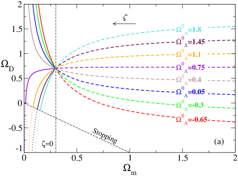
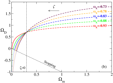
Figure 15: Phase trajectories of the autonomous system (5) in the $(\Omega_{D},\Omega_{m})$ plane. Cases (a) and (b) are respectively as in Figs. 14a,b but here we plot the corresponding trajectories in the phase plane for the total dark energy density versus matter density, i.e. $(\Omega_{D},\Omega_{M})$. The meaning of the lines is as in Fig. 14.

7.7 Phase trajectories of the cosmological autonomous system

Finally, in Fig. 14 and 15 we show some phase trajectories of the autonomous system (5) in two different planes and for particular scenarios covering the two types of situations (node and a saddle point). Due to the stopping conditions discussed in Section 5, in both of these cases the trajectories become eventually truncated and therefore either did not have a chance to reach the convergence node, or alternatively fail to escape away to infinity, respectively. In Figs. 14a,b we display several phase trajectories in the $(\Omega_{\Lambda},\Omega_{X})$ plane covering these possibilities. In Fig. 14a  we have an example that fits with scenario VII of Section 5. The trajectories that turn left and get stopped are those fulfilling the condition (87), whereas those turning right do not fulfill it and hence do not stop. In contrast, in Fig. 14b  we are dealing with scenario IV, where in the absence of stopping the trajectories would be attracted to the node (79) for all values of $\omega_{X}$ in the quintessence range ($\omega_{X}\gtrsim-1$). In this particular example, which illustrates a situation where $\Omega_{\Lambda}^{0}$ and $\nu$ are both rather large, the fixed point is well out of the figure. Even so the trajectories show already a clear trend to get focused. The choice of the parameters does satisfy the stopping condition (80) and so the trajectories get stopped well before reaching the node. It can be clearly seen in the figure because the “stopped part” of the trajectories is partially shown.

In Figs. 15a,b  we represent respectively the same kind of scenarios as in Fig. 14a,b  except that we perform the representation in the plane of total DE density versus matter density. In Fig. 15a the trajectories $\Omega_{D}$ satisfying the condition (87) are seen to get stopped when crossing the straight line $\Omega_{D}=-\Omega_{M}$ corresponding to $r=-1$. The trajectories that do not fulfill (87) escape away into unbounded values of $\Omega_{D}$. Similarly, in Fig. 15b we have a situation with the presence of a “would be node” which focus all trajectories, but all of them get stopped because the condition (80) is fulfilled.

8 Discussion and conclusions

In this paper we have explored the possibilities offered to cosmology by a non-trivial composite model of the dark energy ($\Lambda$XCDM). By composite model we mean that it contains at least two entities of entirely different nature, i.e. not just a replica of a given one (e.g. two or more scalar fields). By non-trivial we mean that these two components generally interact with one another. From our point of view it is perfectly conceivable that the observed DE is made out of a mixture of various components (perhaps some scalar fields) stemming from different sources of a fundamental theory, e.g. string theory. However, in the most general case we have to contemplate the possibility that one of the ingredients of the DE could be a cosmological term, $\Lambda$, with its own dynamics and interactions with the rest. In our model the DE components other than $\Lambda$ have been represented by $X$, the “cosmon”. We should stress that the cosmon need not be a fundamental field, it could be an effective representation of dynamical fields of various sorts, or even the effective behavior of higher order curvature terms in the effective action. In this paper we have presented a composite DE model of this kind, which we have narrowed down to its simplest non-trivial form. The dynamics of the variable cosmological term, $\Lambda$, is linked to the renormalization group (RG) running in QFT, and the effective entity $X$ interacts with $\Lambda$, but not with matter, such that both the total DE and matter-radiation densities are separately conserved. In fact, the cosmon (whose ultimate nature is not necessary to specify in our discussion) follows an evolution which is fixed by the RG dynamics of $\Lambda$ itself through the requirement of conservation of the total DE. The particular modeling of the $\Lambda$ evolution that we have used follows the law $\delta\Lambda\sim H^{2}$, which is well-motivated in the RG framework of Ref. [20, 23, 45]. The modeling could of course be different in other implementations of the RG in Cosmology, or even without explicit reference to it. In this sense the class of $\Lambda$XCDM models is surely more general. However, the non-trivial implementation presented here furnishes a “proof of existence” of promising scenarios of this kind, and suggests that the idea of having a “scaling $\Lambda$” may constitute a fruitful interface between QFT and Cosmology [20]. At the very least it gives a hint on the immense capability of the $\Lambda$XCDM cosmologies to describe the next generation of high precision data, even without making explicit use of simple scalar field models of the DE with particular forms of their potentials.

In the $\Lambda$XCDM context the $\Lambda$ term has a very different status as compared to the $\Lambda$CDM model. While the main observable quantity here is the total DE density $\rho_{D}=\rho_{\Lambda}+\rho_{X}$, the $\Lambda$XCDM model places $\Lambda$ in a fully dynamical context together with the cosmon. Within this approach the puzzling question, formulated within the standard $\Lambda$CDM model, of why $\Lambda$ takes a particular value at present, and why this value is so close to the matter energy density, does no longer apply. The total DE is an evolving quantity through the entire history of the Universe, and under appropriate conditions it traces closely the matter density. This is so because in this model we can find a large region of the parameter space where the expansion of the Universe stops at some point in the future. In contradistinction to the standard $\Lambda$CDM model, here the ratio $\rho_{D}/\rho_{m}$ is not divergent with the evolution, and it reaches a maximum at some point in our future before the Universe stops and reverses its motion. We may view the present state of our Universe in this model as just being in transit to reach that maximum and the subsequent stopping/turning point. At present that ratio is of order $1$, but at the maximum it can be, say, ten times bigger.

Obviously, this framework provides some clue for understanding the cosmological coincidence problem. From our point of view this problem is not so much the issue of why $\rho_{D}/\rho_{m}$ is of order one at present, but rather of why $\rho_{D}/\rho_{m}\rightarrow\infty$ in the asymptotic future regime (as within the standard $\Lambda$CDM model). If that ratio is bounded, as it is the case in the model under consideration, then the Universe can be at any value below this maximum, and this feature certainly improves the status of the purported cosmological coincidence. Within the $\Lambda$XCDM model the fact that $\rho_{D}/\rho_{m}\sim 1$ can be looked upon as a reflex of the present state of accelerated expansion of the Universe, which started somewhere between $z=0.3-0.7$, cf. Eq.  (124). This interpretation is not possible in the standard $\Lambda$CDM model because once the situation $\rho_{D}/\rho_{m}\sim 1$ is reached the ratio further increases without end, and so it is hard to understand why at present this ratio comes out to be of order one. It can only be if we admit that we live in a very special moment, namely one rather close to the start of the acceleration. Similar problems are met by the quintessence and phantom models in the literature. In the former case we cannot understand why the (slowly ever-decreasing) quintessence field matches up the (fast decreasing) matter density precisely right now in the context of an eternal Universe, whereas in the latter we cannot figure out why the (slowly ever-increasing) phantom field just catches up with the matter density squarely around our time.

Quite in contrast, in the $\Lambda$XCDM model, with non-vanishing $\nu$, the ratio $\rho_{D}/\rho_{m}$ remained relatively small in the remote past, being roughly proportional to $|\nu\,(1+\omega_{X})|$. (We can easily provide values of the parameters for which $\rho_{D}/\rho_{m}\sim 10\%$ at the nucleosynthesis era.) Later on, it started to be of order $1$ around the transition epoch ($z=0.3-0.7$) where the Universe changed from a decelerated expansion into an accelerated one. From the early times up to the present day the ratio increased slowly, and in the future it will continue increasing, but it will never surpass a finite number, e.g. of order $10$, until the Universe will stop and reverse its motion (a few Hubble times after our time). The upshot is that from the time of primordial nucleosynthesis till the remote point in the future where the ratio $\rho_{D}/\rho_{m}$ becomes maximum, it changed only mildly, say from $0.1$ to $10$, being currently around $1$, in contrast to the fantastic change predicted in the $\Lambda$CDM case (viz. from $0$ to $\infty$) during its infinite lifetime. Therefore, once the $\Lambda$XCDM Universe starts to accelerate, the probability to live at a time where $r$ is of order $1$ is essentially $1$. Obviously, this model can significantly ameliorate the situation with the cosmological coincidence problem, and it may actually serve as a prototype example of how to reach an explanation for this “coincidence” through the addition of some $X$ to $\Lambda$CDM.

Furthermore, we have shown that the effective EOS behavior of the $\Lambda$XCDM model can mimic to a high extent that of the standard $\Lambda$CDM model (namely by providing an average value of the effective EOS parameter $\omega_{e}$ near $-1$) in essentially the entire redshift interval where the SNAP experiment [7] is going to search for distant supernovae in the near future. Moreover, the possibility of interaction between the cosmon and the cosmological term (which is gauged by the parameter $\nu$) allows to modulate the effective EOS of the $\Lambda$XCDM model by giving it a tilt into the quintessence or phantom regime depending on the sign and size of $\nu$ and the value of the barotropic index of the cosmon, $\omega_{X}$. With no interaction ($\nu=0$) between the two components of the DE, this would be impossible. This shows that even though $\Omega_{\Lambda}$ and $\Omega_{X}$ may not be individually observable, the interaction between $\Lambda$ and $X$ can be detected through the effective EOS features that it gives rise to.

We wish to stand out another important signature of the model that involves comparing the two main ranges of redshift observations. Remarkably, while the behavior of the effective EOS of the $\Lambda$XCDM model at small and intermediate redshifts (relevant to the supernovae analysis) can be very close to the standard $\Lambda$CDM model, it turns out that at the very high redshift range (relevant for CMB considerations) the effective EOS of the DE is similar to that of matter-radiation. In this range the DE physical effects of the $\Lambda$XCDM model could be detected through a “renormalization” correction of the cosmological mass parameter $\Omega_{m}^{0}$ (which could be up to order $10\%$) as compared with the value fitted from the supernovae data. It turns out that most of the parametrizations used in the literature to (simultaneously) fit the effective EOS of the DE at low and high $z$ could be inadequate to describe the $\Lambda$XCDM model and other promising RG cosmological models whose EOS behavior exhibits this kind of features [37].

We may wonder if an effective description of the composite dark energy used in the $\Lambda$XCDM model can be performed in terms of two or more interacting scalar fields. The problem essentially boils down to finding an appropriate potential for the scalar fields. Should the form of this potential be a very complicated or a contrived one, the effective description in terms of scalar fields would not be very appealing. A simple example shows that the scalar field description is not always attractive. Take the special case of the $\Lambda$XCDM model in which $\nu=0$, i.e. the dark energy components do not mutually interact; in particular, we could think of one component being a negative $\Lambda$ and the other being e.g. a quintessence component $X$. In this case an effective description in terms of two non-interacting scalar fields would not be especially useful since one of the fields would have to be non-dynamical. If on the other hand they would be taken as interactive, this would lead to an unnecessarily more complicated scalar field description of the DE as compared to the original $\Lambda$XCDM one, and therefore it could not be considered as a better option. Furthermore, even if an effective scalar field model is found which reproduces the global expansion of the universe in the $\Lambda$XCDM model, local properties such as growth of perturbations might be different in these models. As we stressed before, the cosmon entity need not be a fundamental field. In this sense the $\Lambda$XCDM model can be the effective behavior of many possible constructions, which in all cases have in common the existence of a conserved total DE density. This warns us that we should be careful to avoid extracting too precipitated conclusions on the ultimate nature (e.g. scalar field) of the DE.

Clearly, the $\Lambda$XCDM model can encompass very general behaviors of the DE. Therefore, the fact that the standard $\Lambda$CDM with a strictly constant $\Lambda$ seems to be in fairly good agreement with the last round of high precision WMAP experiments [5] – with the possibility that future SNAP data could independently corroborate this result – in no way can be considered a definitive confirmation of the $\Lambda$CDM. As shown in this paper, the $\Lambda$XCDM model could do in principle a very similar job, with the bonus that it can offer a natural explanation for the cosmological coincidence problem. It remains to study its implications for the structure formation and CMB, but this is of course a task beyond the scope of the present paper. For the moment we have shown that the model can be perfectly tested by performing measurements at all accessible ranges of cosmologically significant redshifts (both low and high), and therefore we expect that the next generation of high precision experiments [7, 8, 9] will allow to better pin down the features of the effective EOS of the dark energy such that the $\Lambda$XCDM parameters can be better determined.

We conclude with the following observation. The “addition” of a dynamical cosmon $X$ to the standard $\Lambda$CDM model can be viewed (or not) as a natural feature in DE model building. But in practice a cosmon-like entity (e.g. in quintessence regime) has thrived alone through the literature quite successfully (as a full substitute for $\Lambda$) for quite some time, following perhaps the courageous – and certainly longer – tradition of $\Lambda$ itself. On the other hand, one may ponder whether it is natural or not to allow a dynamical $\Lambda$ term. However, the running of $\Lambda$, or of any other parameter, may be viewed as a natural property of Quantum Field Theory applied to Cosmology [20]. At the end of the day it seems that other cosmological problems could be significantly smoothed out if the DE is permitted to be neither pure $\Lambda$ nor pure $X$, but just some more or less democratic combination of both, including some peaceful interaction between them.

Acknowledgments: This work has been supported in part by MECYT and FEDER under project 2004-04582-C02-01, and also by DURSI Generalitat de Catalunya under project 2005SGR00564. JG was also supported by project BES-2005-7803. The work of HS is financed by the Secretaría de Estado de Universidades e Investigación of the Ministerio de Educación y Ciencia of Spain within the program Ayudas para la mobilidad de profesores, investigadores, doctores y tecnólogos extranjeros en España. HS thanks the Dep. ECM of the Univ. of Barcelona for the hospitality.

References

- [1] P.J.E. Peebles, Astrophys. J. 284 (1984) 439.
- [2] A.G. Riess et al., Astronom. J. 116 (1998) 1009; S. Perlmutter et al., Astrophys. J. 517 (1999) 565; R. A. Knop et al., Astrophys. J. 598 (2003) 102; A.G. Riess et al. Astrophys. J. 607 (2004) 665.
- [3] D. N. Spergel et al., Astrophys. J. Suppl. 148 (2003) 175; See also the WMAP Collaboration: http://map.gsfc.nasa.gov/
- [4] M. Tegmark et al, Phys. Rev. D69 (2004) 103501.
- [5] WMAP three year results: implications for cosmology, D.N. Spergel et al., astro-ph/0603449.
- [6] M. S. Turner, M. J. White, Phys. Rev. D56 (1997) 4439, astro-ph/9701138.
- [7] See all the relevant information for SNAP in: http://snap.lbl.gov/
- [8] See the relevant information for PLANCK in: http://www.rssd.esa.int/index.php?project=Planck
- [9] The Dark Energy Survey Collaboration, astro-ph/0510346; see also the DES website http://www.darkenergysurvey.org/
- [10] J. Kratochvil, A. Linde, E. V. Linder, M. Shmakova, J. of Cosmology and Astrop. Phys. JCAP 0407 (2004) 001, astro-ph/0312183.
- [11] U. Alam, V. Sahni, A.A. Starobinsky, JCAP 0406 (2004) 008; U. Alam, V. Sahni, T.D. Saini, A.A. Starobinsky, Mon. Not.Roy. Astron. Soc. 354 (2004) 275.
- [12] S. Hannestad, E. Mortsell, JCAP 0409 (2004) 001.
- [13] H.K. Jassal, J.S. Bagla, T. Padmanabhan, Mon. Not. Roy. Astron. Soc. Letters 356 (2005) L11-L16, astro-ph/0404378; Phys. Rev. D72 (2005) 103503, astro-ph/0506748.
- [14] K. M. Wilson, G. Chen, B. Ratra, astro-ph/0602321; H.K. Jassal, J.S. Bagla, T. Padmanabhan, astro-ph/0601389; G.B Zhao, J.Q. Xia, B. Feng, X. Zhang ,Mon. Not.Roy. Astron. Soc. 367 (2006) 825-837, astro-ph/0603621; S. Nesseris, L. Perivolaropoulos, Phys. Rev. D72 (2005) 123519, astro-ph/0511040.
- [15] R.R. Caldwell, Phys. Lett. 545B (2002) 23, astro-ph/9908168; R.R. Caldwell, M. Kamionkowski, N.N. Weinberg, Phys. Rev. Lett. 91 (2003) 071301, astro-ph/0302506; A. Melchiorri, L. Mersini, C.J. Odman, M. Trodden, Phys. Rev. D68 (2003) 043509, astro-ph/0211522; H. Štefančić, Phys. Lett. 586B (2004) 5, astro-ph/0310904; Eur. Phys. J C36 (2004) 523, astro-ph/0312484; Phys. Rev. D71 (2005) 124036, astro-ph/0504518; S. Nojiri, S.D. Odintsov, Phys. Rev. D70 (2004) 103522; S. Capozziello, S. Nojiri, S.D. Odintsov, Phys. Lett. 632B (2006) 597, hep-th/0507182; B. Feng, X. L. Wang, X. M. Zhang, Phys. Lett. 607B (2005) 35, astro-ph/0404224; B. Feng, astro-ph/0602156.
- [16] S. Weinberg, Rev. Mod. Phys. 61 (1989) 1.
- [17] See e.g. V. Sahni, A. Starobinsky, Int. J. of Mod. Phys. A9 (2000) 373; S.M. Carroll, Living Rev. Rel. 4 (2001) 1; T. Padmanabhan, Phys. Rep 380 (2003) 235.
- [18] T. Padmanabhan, Dark Energy: the Cosmological Challenge of the Millennium, Current Science, 88 (2005) 1057, astro-ph/0411044.
- [19] E.J. Copeland, M. Sami, S. Tsujikawa, Dynamics of dark energy, hep-th/0603057.
- [20] I.L. Shapiro, J. Solà, 2002 006, hep-th/0012227; Phys. Lett. 475B (2000) 236, hep-ph/9910462.
- [21] J. Solà, Nucl. Phys. Proc. Suppl. 95 (2001) 29, hep-ph/0101134
- [22] J.A. Gu, W-Y.P. Hwang Phys. Rev. D73 (2003) 023519 astro-ph/0106387; R. Cardenas, T. Gonzalez, O. Martin, I. Quiros Phys. Rev. D67 (2003) 083501, astro-ph/0206315.
- [23] I.L. Shapiro, J. Solà, C. España-Bonet, P. Ruiz-Lapuente, Phys. Lett. 574B (2003) 149, astro-ph/0303306; JCAP 0402 (2004) 006, hep-ph/0311171; I.L. Shapiro, J. Solà, Nucl. Phys. Proc. Supp. 127 (2004) 71, hep-ph/0305279; I. L. Shapiro, J. Solà, JHEP proc. AHEP2003/013, astro-ph/0401015.
- [24] S. Hellerman, N. Kaloper, L. Susskind, 2001003, hep-th/0104180; W. Fischler, A. Kashani-Poor, R. McNees, S. Paban, 2001003, hep-th/0104181; T. Banks, M. Dine 2001 012, hep-th/0106276.
- [25] A.D. Dolgov, in: The very Early Universe, Ed. G. Gibbons, S.W. Hawking, S.T. Tiklos (Cambridge U., 1982); F. Wilczek, Phys. Rep 104 (1984) 143; T. Banks, Nucl. Phys. B249 (1985) 332; L. Abbott, Phys. Lett. B150 (1985) 427; S. M. Barr, Phys. Rev. D36 (1987) 1691; L.H. Ford, Phys. Rev. D 35 (1987) 2339; T.P. Singh and T. Padmanabhan, Int. J. of Mod. Phys. A3 (1988) 1593.
- [26] R.D. Peccei, J. Solà, C. Wetterich, Phys. Lett. 195B (1987) 183; C. Wetterich, Nucl. Phys. B302 (1988) 668; J. Solà, Phys. Lett. 228B (1989) 317; Int. J. of Mod. Phys. A5 (1990) 4225.
- [27] B. Ratra, P.J.E. Peebles, Phys. Rev. D37 (1988) 3406; C. Wetterich, Nucl. Phys. B302 (1988) 668.
- [28] R.R. Caldwell, R. Dave, P.J. Steinhardt, Phys. Rev. Lett. 80 (1998) 1582; For a review, see e.g. P.J.E. Peebles, B. Ratra, Rev. Mod. Phys. 75 (2003) 559, and the long list of references therein.
- [29] C. Deffayet, G.R. Dvali, G. Gabadadze, Phys. Rev. D65 (2002) 044023 ,astro-ph/0105068.
- [30] A. Yu. Kamenshchik, U. Moschella, V. Pasquier, Phys. Lett. 511B (2001) 265, gr-qc/0103004; N. Bilic, G.B. Tupper, R.D. Viollier, Phys. Lett. B 535 (2002) 17, astro-ph/0111325; J.C. Fabris, S.V.B. Goncalves, P.E. de Souza, Gen. Rel. Grav. 34 (2002) 53, gr-qc/0103083; M.C. Bento, O. Bertolami, A.A. Sen, Phys. Rev. D66 (2002) 043507, gr-qc/0202064.
- [31] S. M. Barr, S. Ng, R. J. Scherrer, hep-ph/0601053.
- [32] I.L. Shapiro, J. Solà, Phys. Lett. 475B (2000) 236, hep-ph/9910462.
- [33] C.G. Boehmer, T. Harko, gr-qc/0602081 (to appear in Mod. Phys. Lett. A).
- [34] R.D. Peccei, Phys. Rev. D71 (2005) 023527, hep-ph/0411137; R. Fardon, A.E. Nelson, N. Weiner, J. of Cosmology and Astrop. Phys. JCAP 10 (2004) 005, astro-ph/0309800; P. Gu, X. Wang, X. Zhang, Phys. Rev. D68 (2003) 087301, hep-ph/0307148; P.Q. Hung, hep-ph/0010126.
- [35] S.W. Hawking, G.F.R. Ellis, The Large Scale Structure of Space-Time (Cambridge Univ. Press, 1973); S. M. Carroll, M. Hoffman, M, Trodden, Phys. Rev. D68 (2003) 023509, astro-ph/0301273.
- [36] V. Sahni, T. D. Saini, A. A. Starobinsky, U. Alam, JETP Lett. 77 (2003) 201, Pisma Zh. Eksp. Teor. Fiz. 77 (2003) 249, astro-ph/0201498; Mon. Not.Roy. Astron. Soc. 344 (2003) 1057, astro-ph/0303009; J. A. Frieman, D. Huterer, E. V. Linder, M. S. Turner, Phys. Rev. D67 (2003) 083505, astro-ph/0208100; E.V. Linder, Phys. Rev. D70 (2004) 023511, astro-ph/0402503; E.V. Linder, A. Jenkins, Mon. Not.Roy. Astron. Soc. 346 (2003) 573, astro-ph/0305286.
- [37] J. Solà, H. Štefančić, Phys. Lett. 624B (2005) 147, astro-ph/0505133.
- [38] J. Solà, H. Štefančić, Mod. Phys. Lett. A21 (2006) 479, astro-ph/0507110; J. Phys. A39 (2006) 6753, gr-qc/0601012; J. Solà, J. Phys. Conf. Ser. 39 (2006) 179, gr-qc/0512030.
- [39] B. Guberina, R. Horvat, H. Nikolic, astro-ph/0601598.
- [40] P.J. Steinhardt, in: Proc. of the 250th Anniversary Conference on Critical Problems in Physics, ed. V.L. Fitch, D.R. Marlow, M.A.E. Dementi (Princeton Univ. Pr., Princeton, 1997).
- [41] L. Amendola, Phys. Rev. D62 (2000) 043511, astro-ph/9908023; L. Amendola, D. Tocchini-Valentini, Phys. Rev. D64 (2001) 043509, astro-ph/0011243; W. Zimdahl, D. Pavon, Phys. Lett. 521B (2001) 133, astro-ph/0105479; J.P. Uzan, Phys. Rev. D59 (1999) 123510, gr-qc/9903004.
- [42] S. Dodelson, M. Kaplinghat, E. Stewart, Phys. Rev. Lett. 85 (2000) 5276, astro-ph/0002360; B. Feng, M. Li, Y.S. Piao, X. Zhang, Phys. Lett. 634B (2006 ) 101, astro-ph/0407432; K. Griest, Phys. Rev. D66 (2002) 123501, astro-ph/0202052; E. V. Linder, Astropart. Phys. 25 (2006) 167, astro-ph/0511415; S. Nojiri, S. D. Odintsov, hep-th/0603062.
- [43] R. J. Scherrer, Phys. Rev. D71 (2005) 063519, astro-ph/0410508.
- [44] I.L. Buchbinder, S.D. Odintsov and I.L. Shapiro, Effective Action in Quantum Gravity, IOP Publishing (Bristol, 1992); N.D. Birrell and P.C.W. Davies, Quantum Fields in Curved Space, Cambridge Univ. Press (Cambridge, 1982).
- [45] I.L. Shapiro, J. Solà, H. Štefančić, JCAP 0501 (2005) 012 , hep-ph/0410095.
- [46] A. Babic, B. Guberina, R. Horvat, H. Štefančić, Phys. Rev. D65 (2002) 085002; B. Guberina, R. Horvat, H. Štefančić Phys. Rev. D67 (2003) 083001; A. Babic, B. Guberina, R. Horvat, H. Stefancic, Phys. Rev. D71 (2005) 124041,astro-ph/0407572; B. Guberina, R. Horvat, H. Štefančić, J. of Cosmology and Astrop. Phys. JCAP 05 (2005) 001, astro-ph/0503495.
- [47] A. Bonanno, M. Reuter, Phys. Rev. D65 (2002) 043508; E. Bentivegna, A. Bonanno, M. Reuter, J. of Cosmology and Astrop. Phys. JCAP 01 (2004) 001.
- [48] F. Bauer, Class. Quant. Grav. 22 (2005) 3533, gr-qc/0501078; F. Bauer, gr-qc/0512007.
- [49] M. Reuter, C. Wetterich, Phys. Lett. 188B (1987) 38; K. Freese, F. C. Adams, J. A. Frieman, E. Mottola, Nucl. Phys. B287 (1987) 797; P.J.E. Peebles, B. Ratra, Astrophys. J. L17 (1988) 325; J.C. Carvalho, J.A.S. Lima, I. Waga, Phys. Rev. D46 (1992) 2404; O. Bertolami 1986, Nuovo Cim. B93 (1986)36.
- [50] See e.g. J.M. Overduin, F. I. Cooperstock, Phys. Rev. D58 (1998) 043506 and R.G. Vishwakarma, Class. Quant. Grav. 18 (2001) 1159.
- [51] T. Barreiro, E.J. Copeland, N.J. Nunes, Phys. Rev. D61 (2000) 127301
- [52] B. McInnes 2002029, hep-th/0112066.
- [53] J. Ren, X.H. Meng, astro-ph/0602462.
- [54] P. G. Ferreira, M. Joyce, Phys. Rev. D58 (1998) 023503, astro-ph/9711102.
- [55] S. Carneiro, Int. J. of Mod. Phys. D14 (2005) 2201, gr-qc/0505121.