Quasi-particle creation by
analogue black holes

Abstract

We discuss the issue of quasi-particle production by “analogue black holes” with particular attention to the possibility of reproducing Hawking radiation in a laboratory. By constructing simple geometric acoustic models, we obtain a somewhat unexpected result: We show that in order to obtain a stationary and Planckian emission of quasi-particles, it is not necessary to create an ergoregion in the acoustic spacetime (corresponding to a supersonic regime in the flow). It is sufficient to set up a dynamically changing flow either eventually generating an arbitrarily small sonic region $v=c$, but without any ergoregion, or even just asymptotically, in laboratory time, approaching a sonic regime with sufficient rapidity.

PACS: 04.20.Gz, 04.62.+v, 04.70.-s, 04.70.Dy, 04.80.Cc
Keywords: analogue models, acoustic spacetime, Hawking radiation

1 Introduction

It is by now well established that the physics associated with classical and quantum fields in curved spacetimes can be reproduced, within certain approximations, in a variety of different physical systems — the so-called “analogue models of General Relativity (GR)” [1, 2]. The simplest example of such a system is provided by acoustic disturbances propagating in a barotropic, irrotational and viscosity-free fluid.

In the context of analogue models it is natural to separate the kinematical aspects of GR from the dynamical ones. In general, within a sufficiently complex analogue model one can reproduce any pre-specified spacetime — and the kinematics of fields evolving on it — independently of whether or not it satisfies the classical (or semiclassical) Einstein equations [3]. Indeed, to date there are no analogue models whose effective geometry is determined by Einstein equations. In this sense we currently have both analogue spacetimes and analogues of quantum field theory in curved spacetimes, but (strictly speaking) no analogue model for GR itself [4].

In order to reproduce a specific spacetime geometry within an analogue model, one would have to take advantage of the specific equations describing the latter (for example, for fluid models, the Euler and continuity equations, together with an equation of state), plus the possibility of manipulating the system by applying appropriate external forces. In the analysis of this paper we will think of the spacetime configuration as “externally given”, assuming that it has been set up as desired by external means — any back-reaction on the geometry is neglected as in principle we can counter-balance its effects using the external forces. In the context of analogue models this is not merely a hypothesis introduced solely for theoretical simplicity, but rather a realistic situation that is in principle quite achievable.

Specifically, in this paper we analyze in simple terms the issue of quantum quasi-particle creation by several externally specified $(1+1)$-dimensional analogue geometries simulating the formation of black hole-like configurations. (In a previous companion paper [5] we investigated the causal structure of these, and other, spacetimes.) In this analysis we have in mind, on the one hand, the possibility of setting up laboratory experiments exhibiting Hawking-like radiation [6, 7] and, on the other hand, the acquisition of new insights into the physics of black hole evaporation in semiclassical gravity. All the discussion holds for a scalar field obeying the D’Alembert wave equation in a curved spacetime. This means that we are not (for current purposes) considering the deviations from the phononic dispersion relations that show up at high energies owing to the atomic structure underlying any condensed matter system. We shall briefly comment on these modifications at the end of the paper. For simplicity, throughout the paper we adopt a terminology based on acoustics in moving fluids (we will use terms such as acoustic spacetimes, sonic points, fluid velocity, etc.), but our results are far more general and apply to many other analogue gravity models not based on acoustics. We summarise the main conclusions below.

First of all, we recover the standard Hawking result when considering fluid flows that generate a supersonic regime at finite time. (That is, we recover a stationary creation of quasi-particles with a Planckian spectrum.) We then analyze the quasi-particle creation associated with other types of configurations. In particular, we shall discuss in detail a “critical black hole” — a flow configuration that presents an acoustic horizon without an associated supersonic region. From this analysis we want to highlight two key results:

• The existence of a supersonic regime (sound velocity $c$ strictly smaller than fluid velocity $v$) is not needed in order to reproduce Hawking’s stationary particle creation. We demonstrate this fact by calculating the quantity of quasi-particle production in an evolving geometry which generates only an isolated sonic point ($v=c$), but without a supersonic region, in a finite amount of laboratory time.

• Moreover, in order to produce a Hawking-like effect it is not even necessary to generate a sonic point at finite time. All one needs is that a sonic point develops in the asymptotic future (that is, for $t\to+\infty$) with sufficient rapidity (we shall explain in due course what we exactly mean by this).

From the point of view of the reproducibility of a Hawking-like effect in a laboratory, the latter result is particularly interesting. In general, the formation of a supersonic regime in a fluid flow — normally considered to be the crucial requirement to produce Hawking emission — is associated with various different types of instability (Landau instability in superfluids, quantized vortex formation in Bose–Einstein condensates, etc.) that could mask the Hawking effect. To reproduce a Hawking-like effect without invoking a supersonic regime could alleviate this situation.

From the point of view of GR, we believe that our result could also have some relevance, as it suggests a possible alternative scenario for the formation and semiclassical evaporation of black hole-like objects.

The plan of the paper is the following: In the next section we introduce the various acoustic spacetimes on which we focus our attention, spacetimes that describe the formation of acoustic black holes of different types. In section 4 we present separately the specific calculations of redshift for sound rays that pass asymptotically close to the event horizon of these black holes. By invoking standard techniques of quantum field theory in curved spacetime, one can then immediately say when particle production with a Planckian spectrum takes place. Finally, in the last section of the paper we summarise and discuss the results obtained.

2 Acoustic black holes

Associated with the flow of a barotropic, viscosity-free fluid along an infinitely long thin pipe, with density and velocity fields constant on any cross section orthogonal to the pipe, there is a (1+1)-dimensional acoustic spacetime $({\cal M},{\mbox{\sl g}})$, where the manifold $\cal M$ is diffeomorphic to ${\rm I\!R}^{2}$. Using the laboratory time $t\in{\rm I\!R}$ and physical distance $x\in{\rm I\!R}$ along the pipe as coordinates on $\cal M$, the acoustic metric on $\cal M$ can be written as

$${\mbox{\sl g}}=\Omega^{2}\left[-\left(c^{2}-v^{2}\right){\mathrm{d}}t^{2}+2\,v\,{\mathrm{d}}t\,{\mathrm{d}}x+{\mathrm{d}}x^{2}\right]=\Omega^{2}\left[-c^{2}\,dt^{2}+({\mathrm{d}}x+v\,{\mathrm{d}}t)^{2}\right]\;,$$ (2.1)

where $c$ is the speed of sound, $v$ is the fluid velocity, and $\Omega$ is an unspecified non-vanishing function [8]. In general, all these quantities depend on the laboratory coordinates $x$ and $t$. Here, we shall assume that $c$ is a constant. Hence, it is the velocity $v(x,t)$ that contains all the relevant information about the causal structure of the acoustic spacetime $({\cal M},{\mbox{\sl g}})$. We direct the reader to the companion paper [5] for a detailed analysis of the causal structure associated with a broad class of $(1+1)$-dimensional acoustic geometries, both static and dynamic.

2.1 Apparent horizon

The sonic points, where $v(t,x)=\pm c$, correspond to the so-called acoustic apparent horizons — apparent horizons for the Lorentzian geometry defined on $\cal M$ by the metric (2.1). The fact of having an underlying Minkowski structure associated with the laboratory observer makes the definition of apparent horizons in acoustic models less troublesome than in GR (see e.g. reference [2], pp. 15–16).

Consider a monotonically non-decreasing function $\bar{v}(x)$ such that $\bar{v}(0)=-c$ and $\bar{v}(x)\to 0$ for $x\to+\infty$. If one chooses $v(x,t)=\bar{v}(x)$ in (2.1), the corresponding acoustic spacetime represents, for observers with $x>0$, a static black hole with the horizon located at $x=0$ (in this case apparent and event horizon coincide), a black hole region for $x<0$, and a (right-sided) surface gravity

$$\kappa:=\lim_{x\to 0^{+}}\frac{{\mathrm{d}}\bar{v}(x)}{{\mathrm{d}}x}\;.$$ (2.2)

We can, moreover, distinguish three cases:

• $\kappa\neq 0$ and $\bar{v}(x)<-c$ for $x<0$: a non-extremal black hole;

• $\kappa\neq 0$ and $\bar{v}(x)=-c$ for $x<0$: a “critical” black hole;

• $\kappa=0$ and $\bar{v}(x)=-c$ for $x<0$: an extremal black hole.

Now, taking the above $\bar{v}(x)$, let us consider $t$-dependent velocity functions

$$v(x,t)=\left\{\begin{array}[]{lll}\bar{v}(\xi(t))&\mbox{if}&x\leq\xi(t)\;,\\ \bar{v}(x)&\mbox{if}&x\geq\xi(t)\;,\end{array}\right.$$ (2.3)

with $\xi$ a monotonically decreasing function of $t$, such that $\displaystyle\lim_{t\to-\infty}\xi(t)=+\infty$ and $\displaystyle\lim_{t\to-\infty}\dot{\xi}(t)=0$. (The first condition serves to guarantee that spacetime is flat at early times, whereas we impose the second one only for simplicity. All the analysis in the paper could be performed without adopting this assumption, leaving the physical results unchanged. However, that would require more case-by-case splitting, only to cover new situations without physical interest.) There are basically two possibilities for $\xi$, according to whether the value $\xi=0$ is attained for a finite laboratory time $t_{\rm H}$ or asymptotically for an infinite future value of laboratory time.

In the first case $\xi(t_{\rm H})=0$ and the corresponding metric (2.1) represents the formation of a non-extremal, critical, or extremal black hole, respectively. For small values of $|t-t_{\rm H}|$ we have

$$\xi(t)=-\lambda\,(t-t_{\rm H})+{\cal O}([t-t_{\rm H}]^{2})\;,$$ (2.4)

where $\lambda$ is a positive parameter. Hence the function $\xi$ behaves, qualitatively, as shown in figure 1.

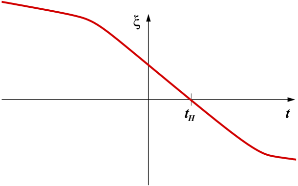
Figure 1: Plot of $\xi(t)$ for the formation of an acoustic apparent horizon at a finite laboratory time $t_{\rm H}$. Only the behaviour of $\xi$ for $t$ close to $t_{\rm H}$ is important.

Apart from this feature, the detailed behaviour of $\xi$ is largely irrelevant for our purposes.

If instead $\xi\to 0$ is attained only at infinite future time, that is $\displaystyle\lim_{t\to+\infty}\xi(t)=0$, one is describing the asymptotic formation of either a critical black hole (if $\kappa\neq 0$; obviously, in this case choosing the non-extremal or the critical $\bar{v}(x)$ profile is irrelevant) or an extremal black hole (if $\kappa=0$). Now the function $\xi$ behaves, qualitatively, as shown in figure 2.

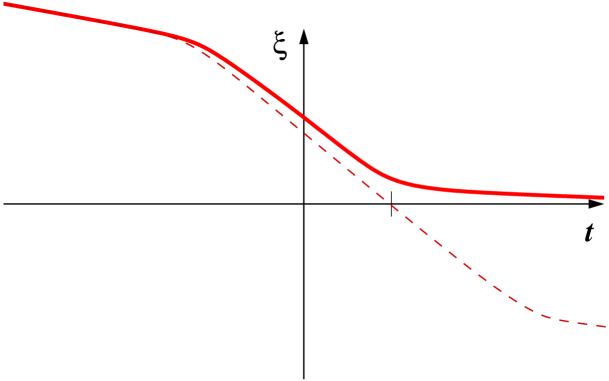
Figure 2: Plot of $\xi(t)$ for the asymptotic formation of an acoustic apparent horizon at infinite future laboratory time. Only the asymptotic behaviour of $\xi$ for $t\to+\infty$ is important. (For comparison we also plot $\xi(t)$, with a dashed line, for the formation of the apparent horizon at finite laboratory time.)

The relevant feature of $\xi(t)$ is its asymptotic behaviour as $t\to+\infty$. In the following we shall consider two possibilities for this asymptotics, although others can, of course, be envisaged:

(i)

Exponential: $\xi(t)\sim A\,{\mathrm{e}}^{-\kappa_{\rm D}\,t}$, with $\kappa_{\rm D}$ a positive constant, in general different from $\kappa$, and $A>0$;

(ii)

Power law: $\xi(t)\sim B\,t^{-\nu}$, with $\nu>0$ and $B>0$.

2.2 Null coordinates

For all the situations considered so far, spacetime is Minkowskian in the two asymptotic regions corresponding to $t\to-\infty$, and to $t\to+\infty$, $x\to+\infty$ (${\Im}^{-}$ and ${\Im}^{+}_{\rm right}$, respectively, adopting the notation of reference [5]). Starting with a quantum scalar field in its natural Minkowskian vacuum at $t\to-\infty$, we want to know the total quantity of quasi-particle production to be detected at the right asymptotic region at late times, $t\to+\infty$, caused by the dynamical evolution of the velocity profile $v(x,t)$.

In the geometric acoustic approximation, a right-going sound ray is an integral curve of the differential equation

$$\frac{{\mathrm{d}}x}{{\mathrm{d}}t}=c+v(x,t)\;.$$ (2.5)

We are interested in sound rays propagating from ${\Im}^{-}$ (see figure 3); that is, in solutions of (2.5) that satisfy an initial condition $x(t_{i})=x_{i}$, with $x_{i}\sim ct_{i}$ in the limit $t_{i}\to-\infty$ (so $P:=(x_{i},t_{i})$ can be thought of as an “initial” event corresponding to the emission of the acoustic signal).

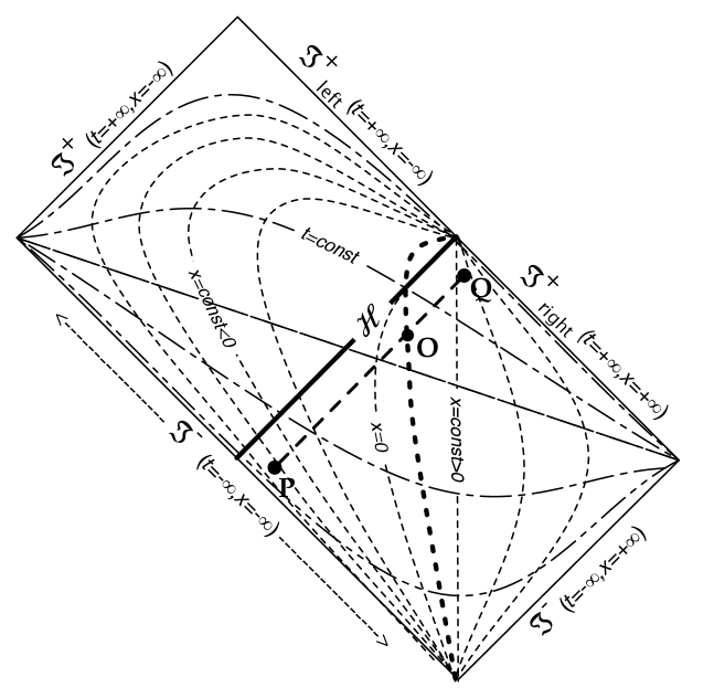
Figure 3: Conformal diagram of the spacetime corresponding to the formation of an acoustic black hole. The dotted line in bold represents the worldline of the kink, $x=\xi(t)$. The dashed straight line in bold represents a right-going ray connecting the events $P=(x_{i},t_{i})$ near ${\Im}^{-}$ and $Q=(x_{f},t_{f})$ near ${\Im}^{+}_{\rm right}$.

If such a ray ends up on ${\Im}^{+}_{\rm right}$, we can identify “final” events $Q:=(x_{f},t_{f})$ on it, with $x_{f}\sim ct_{f}$ as $t_{f}\to+\infty$. For a ray connecting ${\Im}^{-}$ to ${\Im}^{+}_{\rm right}$ one can also find an event $O:=(x_{0},t_{0})$ such that $x_{0}=x(t_{0})=\xi(t_{0})$, which corresponds to the crossing of the “kink” in $v$, located at $x=\xi(t)$ according to equation (2.3), by the sound signal. Finally, we can define, for such a ray, two parameters $U$ and $u$ as follows:

$$U:=\lim_{t_{i}\to-\infty}\left(t_{i}-x_{i}/c\right)\;;$$ (2.6)

$$u:=\lim_{t_{f}\to+\infty}\left(t_{f}-x_{f}/c\right)\;.$$ (2.7)

Such parameters correspond to null coordinates in spacetime. If an acoustic event horizon $\cal H$ is present in the spacetime, the coordinate $U$ is regular on it (i.e., $U$ attains some finite value on $\cal H$), whereas $u$ tends to $+\infty$ as $\mathcal{H}$ is approached.

We can express both $U$ and $u$ in terms of the velocity profile (shape and dynamics) and of the crossing time $t_{0}$. To this end, we can integrate equation (2.5), first between $P$ and $O$:

$$\xi(t_{0})-x_{i}=\int_{t_{i}}^{t_{0}}{\mathrm{d}}t\left(c+\bar{v}(\xi(t))\right)\;;$$ (2.8)

then between $O$ and $Q$:

$$t_{f}-t_{0}=\int_{\xi(t_{0})}^{x_{f}}\frac{{\mathrm{d}}x}{c+\bar{v}(x)}\;.$$ (2.9)

On replacing $x_{i}$ from equation (2.8) into (2.6), we find the value of $U$ for a generic right-moving ray that crosses the kink at laboratory time $t_{0}$:

$$U=t_{0}-\frac{\xi(t_{0})}{c}+\frac{1}{c}\int_{-\infty}^{t_{0}}{\mathrm{d}}t\,\bar{v}(\xi(t))\;.$$ (2.10)

Similarly, substituting $t_{f}$ from equation (2.9) into (2.7), then adding and subtracting the quantity $\xi(t_{0})/c$, we find

$$u=t_{0}-\frac{\xi(t_{0})}{c}-\frac{1}{c}\int_{\xi(t_{0})}^{+\infty}{\mathrm{d}}x\,\frac{\bar{v}(x)}{c+\bar{v}(x)}\;.$$ (2.11)

In the analysis below, our chief goal consists of finding the relation between $U$ and $u$ for a sound ray that is close to the horizon, i.e., in the asymptotic regime $u\to+\infty$. From such a relation it is then a standard procedure to find the Bogoliubov $\beta$ coefficients and hence the total quasi-particle content to be measured, in this case, by an asymptotic observer at ${\Im}^{+}_{\rm right}$. (See, for example, reference [7]). In the case of an exponential relation between $U$ and $u$ it is a well established result that a Planckian spectrum is observed at late times [9], so Hawking-like radiation will be recovered.

3 Event horizon formation

When the apparent horizon forms at a finite laboratory time, say at $t=t_{\rm H}$, an event horizon always exists, generated by the right-moving ray that eventually remains frozen on the apparent horizon, at $x=0$. For such a ray $t_{0}\to t_{\rm H}$, and since $\xi(t_{\rm H})=0$, the $U$ parameter has the finite value

$$U_{\rm H}=t_{\rm H}+\frac{1}{c}\int_{-\infty}^{t_{\rm H}}{\mathrm{d}}t\,\bar{v}(\xi(t))\;.$$ (3.1)

For a ray with $U<U_{\rm H}$ we then obtain, combining equations (2.10) and (3.1):

$$U=U_{\rm H}+t_{0}-t_{\rm H}-\frac{\xi(t_{0})}{c}-\frac{1}{c}\int_{t_{0}}^{t_{\rm H}}{\mathrm{d}}t\,\bar{v}(\xi(t))\;.$$ (3.2)

This exact equation is now in a form suitable for conveniently extracting approximate results in the region $t_{0}\sim t_{\rm H}$, corresponding to sound rays that “skim” the horizon.

On the other hand, when the trapping horizon consists of just one single sonic point located at $t=+\infty$, it is not obvious that an event horizon exists. Loosely speaking, in this case it might happen that the trapping horizon form “after” every right-going ray from ${\Im}^{-}$ has managed to cross $x=0$. Since there is a competition between two infinite quantities — the time at which the trapping horizon forms, and the time at which the “last” right-going signal that connects $x=-\infty$ with $x=+\infty$ crosses $x=0$ — a careful case-by-case analysis is in order.

This is essentially all that can be said without relying on specific features of $\bar{v}(x)$. We now consider separately the various situations of interest, focussing first on the issue of the existence of the event horizon.

3.1 Non-extremal black hole

In the case of a non-extremal black hole, the qualitative behaviour of the function $\bar{v}(x)$ is shown, graphically, in figure 4.

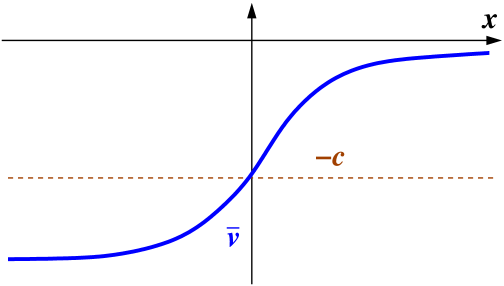
Figure 4: The static velocity profile $\bar{v}(x)$ for an acoustic non-extremal black hole.

Note that, for small values of $|x|$, one can write

$$\bar{v}(x)=-c+\kappa\,x+{\cal O}(x^{2})\;.$$ (3.3)

The function $\xi(t)$ behaves as already shown in figure 1. A sketch of the worldlines of right-moving sound rays is presented in figure 5.

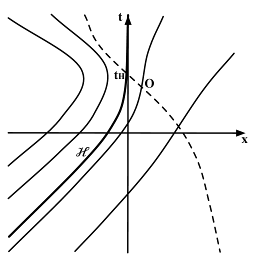
Figure 5: The worldlines of right-moving sound rays in the spacetime describing the formation of a non-critical, non-extremal black hole. The thick solid line is the event horizon; the dashed one is the worldline of the “kink,” $x=\xi(t)$.

Note that in the portion of the diagram to the right of the curve $x=\xi(t)$ (i.e., to the right of the moving kink in the velocity profile), spacetime is static. For $t\to-\infty$, the geometry is Minkowskian and the worldlines tend to approach straight lines with slope $1/c$.

The sound ray that generates the event horizon corresponds to a finite value $U_{\rm H}$ of the coordinate $U$. Hence, in this situation an event horizon always exists. This is also clear from the fact that the vertical half-line $x=0$, $t>t_{\rm H}$ in figure 5 is an apparent horizon.

3.2 Critical black hole

The function $\bar{v}(x)$ behaves as shown in figure 6. Regarding the right side of the profile, $x>0$, it is indistinguishable from the profile of a non-extremal black hole (figure 4).

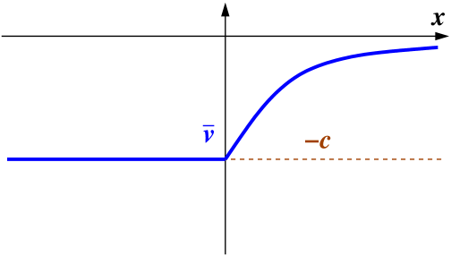
Figure 6: The static velocity profile $\bar{v}(x)$ for a critical black hole.

3.2.1 Finite time

When the function $\xi(t)$ is of the form (2.4), that is, when the apparent horizon is formed at a finite amount of laboratory time, the situation is exactly the same as for the non-extremal black hole discussed above.

3.2.2 Infinite time

Consider now that the sonic point is approached in an infinite amount of time, so the function $\xi(t)$ behaves as in figure 2. The worldlines of right-moving sound rays are shown in figure 7.

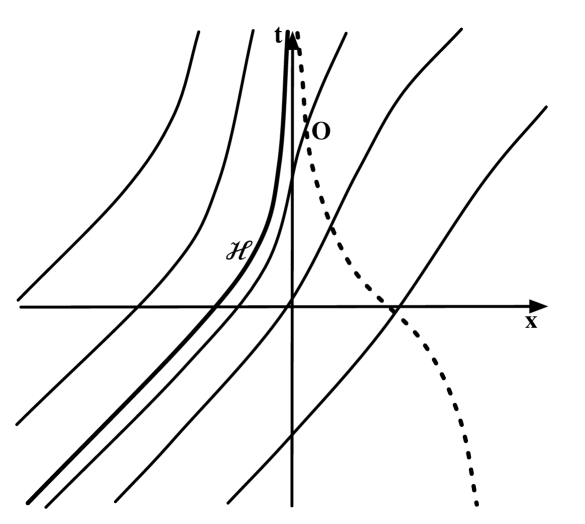
Figure 7: The worldlines of right-moving sound rays in the spacetime describing the formation of a critical black hole. The apparent horizon is just an asymptotic point at $x=0$, $t\to+\infty$. The event horizon, when it exists, corresponds to a line like the thick solid one. The worldline of the kink is dashed. This situation is qualitatively identical to the case of the formation of an extremal black hole in an infinite laboratory time.

As in the formation of the non-critical black hole, the portion of the diagram to the right of the curve $x=\xi(t)$ (i.e., to the right of the moving kink in the velocity profile) corresponds to a static spacetime, and for $t\to-\infty$ the geometry is Minkowskian — the worldlines tend to approach straight lines with slope $1/c$. However, now the apparent horizon is just the asymptotic point located at $x=0$, $t\to+\infty$, and in order to establish whether an event horizon does, or does not, exist one must perform an actual calculation of $U_{\rm H}$ for the “last” ray that crosses the kink. The expression for $U_{\rm H}$ is again obtained from equation (2.10), noticing that now $t_{0}=+\infty$ along the generator of the would-be horizon, so

$$U_{\rm H}=\lim_{t_{0}\to+\infty}\left(t_{0}+\frac{1}{c}\int_{-\infty}^{t_{0}}{\mathrm{d}}t\,\bar{v}\left(\xi(t)\right)\right)\;.$$ (3.4)

The necessary and sufficient condition for the event horizon to exist is that the limit on right hand side of equation (3.4) be finite. The integrand on right hand side of (3.4) can be approximated, for $t\to t_{0}\to+\infty$, as $-c+\kappa\,\xi(t)$, while for $t\to-\infty$ it just approaches zero. Hence $U_{\rm H}$ is, up to a finite constant, equal to $\kappa/c$ times the integral of $\xi$, evaluated at $t\to+\infty$. Here we must distinguish between the exponential behaviour and the power law — cases (i) and (ii). In the former $U_{\rm H}$ is finite, trivially. For the power law, it turns out that $U_{\rm H}$ is finite iff $\nu>1$.

3.3 Extremal black hole

The typical spatial profile function $\bar{v}(x)$ for an extremal black hole is plotted in figure 8.

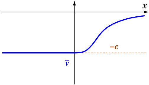
Figure 8: The static velocity profile $\bar{v}(x)$ for an acoustic extremal black hole.

For $x$ approaching zero from positive values we can write

$$\bar{v}(x)=-c+\mu\,x^{2}+{\cal O}(x^{3})\;,$$ (3.5)

where $\mu>0$ is a constant. As far as dynamics is concerned, we must distinguish the cases in which the apparent horizon is formed at finite laboratory time $t_{\rm H}$, and in an infinite time (i.e., for $t\to+\infty$).

3.3.1 Finite time

The function $\xi(t)$ is of the type shown in figure 1, and the worldlines of right-going sound rays are sketched in figure 9.

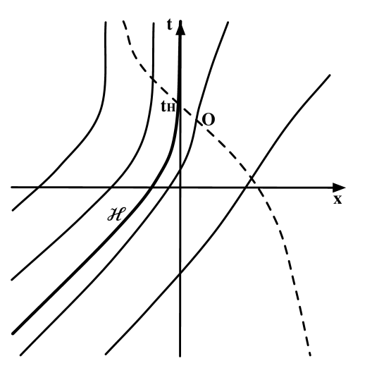
Figure 9: The worldlines of right-moving sound rays in the spacetime describing the formation of an extremal black hole in a finite laboratory time. The thick solid and dashed lines represent, respectively, the event horizon and the worldline of the kink.

The event horizon always exists.

3.3.2 Infinite time

The function $\xi(t)$ is as shown in figure 2, and the worldlines of right-going signals are shown in figure 7. As in the case of the formation of a critical black hole, the apparent horizon forms only asymptotically, for $x=0$ and $t\to+\infty$, so the event horizon exists iff $U_{\rm H}$, given by equation (3.4), has a finite value. Using the expansion (3.5) in equation (3.4), one finds that $U_{\rm H}$ is always finite when $\xi(t)$ is asymptotically exponential. On the other hand, for a power law, the event horizon exists iff $\nu>1/2$. (Note that the critical value of the exponent, $\nu=1/2$, is now not the same as for the critical black hole, $\nu=1$.)

3.4 Double-sided black hole configurations

The configurations we have analyzed until now are the simplest from a purely mathematical point of view. However, having in mind acoustic analogue geometries reproducible in a one-dimensional pipe in the laboratory, it is more sensible to consider double-sided configurations. By this we mean that, after passing (or approaching) the sonic/supersonic regime at $x=0$, and traversing an interval of width $I\geq 0$, the fluid again goes back to a subsonic regime as $x\to-\infty$.

Consider for example functions $\bar{v}(x)$ such that $\bar{v}(x)=-c$ for $-I\leq x\leq 0$,

$$\lim_{x\to-I^{-}}\frac{{\mathrm{d}}\bar{v}(x)}{{\mathrm{d}}x}\neq 0\;,~{}~{}~{}~{}~{}\lim_{x\to 0^{+}}\frac{{\mathrm{d}}\bar{v}(x)}{{\mathrm{d}}x}\neq 0\;,$$ (3.6)

and which outside the interval $-I\leq x\leq 0$ tend monotonically to zero as $|x|$ increases (see figures 10 and 11).

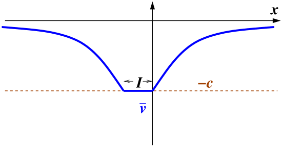
Figure 10: The static velocity profile $\bar{v}(x)$ for a double-sided critical black hole. $I$ indicates the size of the internal flat segment.

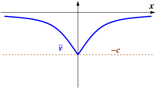
Figure 11: The static velocity profile $\bar{v}(x)$ for a double-sided critical black hole with zero “thickness” ($I=0$).

The corresponding fluid configuration represents what could be called a static “double-sided critical black hole”. The formation of such a configuration can be modelled by the velocity function

$$v(x,t)=\left\{\begin{array}[]{lll}\bar{v}(x)&\mbox{if}&x\geq\xi(t)\;,\\ \bar{v}(\xi(t))&\mbox{if}&-I-\xi(t)\leq x\leq\xi(t)\;,\\ \bar{v}(x)&\mbox{if}&x\leq-I-\xi(t)\;,\end{array}\right.$$ (3.7)

with $\xi$ a monotonically decreasing function of $t$, and $\bar{v}$ as above. Accordingly, the differential equation for right-going sound rays also splits:

$$\frac{{\mathrm{d}}x}{{\mathrm{d}}t}=\left\{\begin{array}[]{lll}c+\bar{v}(x)&\mbox{if}&x\geq\xi(t)\;.\\ c+\bar{v}(\xi(t))&\mbox{if}&-I-\xi(t)\leq x\leq\xi(t)\;,\\ c+\bar{v}(x)&\mbox{if}&x\leq-I-\xi(t)\;.\end{array}\right.$$ (3.8)

Geometries associated with the formation of non-extremal and extremal black holes can be constructed in the same way; see figures 12 and 13 for plots of the respective $\bar{v}$ functions.

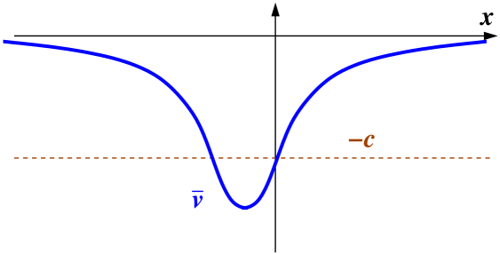
Figure 12: The static velocity profile $\bar{v}(x)$ for a double-sided non-extremal black hole. In the companion paper [5] we refer to this configuration as a black hole-white hole configuration.

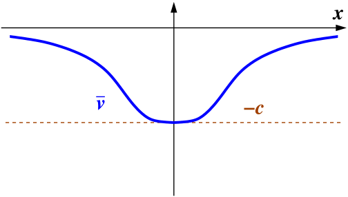
Figure 13: The static velocity profile $\bar{v}(x)$ for a double-sided extremal black hole with zero thickness ($I=0$).

3.4.1 Finite time

The function $\xi(t)$ is of the type illustrated in figure 1. The behaviour of right-going sound rays is shown in figure 14.

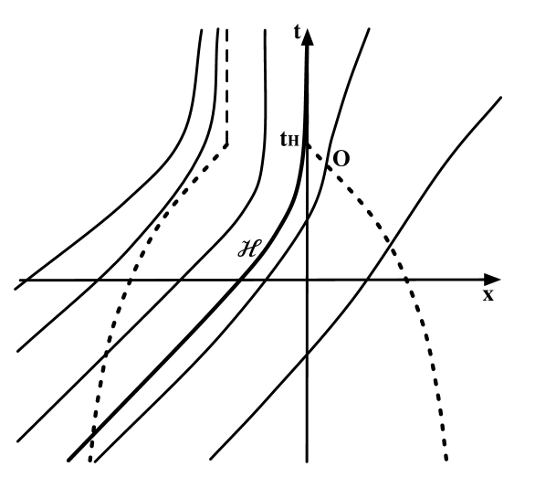
Figure 14: The worldlines of right-moving sound rays in the spacetime describing the formation of a double-sided critical black hole in a finite laboratory time. The event horizon is represented by the thick solid line, while the worldlines of the kinks are dashed.

The apparent horizon is the half-line $x=0$, $t>0$, and the event horizon always exists.

3.4.2 Infinite time

Let us now consider a function $\xi(t)$ of the type illustrated in figure 2. The behaviour of right-going sound rays is shown in figure 15.

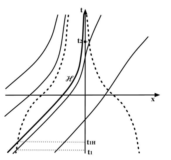
Figure 15: The worldlines of right-moving sound rays in the spacetime describing the formation of a double-sided critical black hole in an infinite laboratory time. The apparent horizon is the asymptotic point $x=0$, $t\to+\infty$. The event horizon (when it exists) is represented by the thick solid line, while the worldlines of the kinks are dashed.

For these particular configurations, whether an event horizon does, or does not, actually exist is now a rather tricky issue. The asymptotic behaviour of the function $\xi(t)$ at $t\to-\infty$ ensures that all the right-going rays start to the left of the right-moving kink (i.e., the one in the region $x<0$), then catch up with it, and begin to propagate through the intermediate region at a velocity $c+\bar{v}(\xi(t))$ that depends only on $t$. Before they reach the point $x=0$, such rays might be overtaken by the right-moving kink, but only to start the chase again. After several mutual overtakings (if the function $\xi(t)$ is sufficiently complicated), the rays will always make an ultimate overtaking of the right-moving kink, embarking upon a final encounter with the left-moving kink on the right (i.e., in the region $x>0$). Let us denote by $t_{1}$ the time of such a last crossing of the right-moving kink, so the corresponding event is $(-\xi(t_{1})-I,t_{1})$. Also, let us denote by $t_{2}$ the time at which the same ray crosses the kink on the right, so that the corresponding event is $(\xi(t_{2}),t_{2})$. From equation (3.8) we directly obtain the relation

$$\xi(t_{1})+I=-\xi(t_{2})+\int_{t_{1}}^{t_{2}}{\mathrm{d}}t\left[c+\bar{v}\left(\xi(t)\right)\right]\;.$$ (3.9)

between $t_{2}$ and $t_{1}$. (When the ray crosses the right-moving kink more than once, equation (3.9) will be satisfied by more than one value of $t_{1}$ for any given $t_{2}$. In order to avoid cumbersome notation, we shall simply denote by $t_{1}$ the largest of these roots, corresponding to the last crossing.) Then a necessary and sufficient condition for the existence of an event horizon is that, for $t_{2}\to+\infty$, $t_{1}$ tends to a finite value, say $t_{1{\rm H}}$. This guarantees that any right-going ray that last crosses the left kink at a time greater than $t_{1{\rm H}}$ does not reach the region $x>0$ (as ray-crossing cannot occur under the working hypothesis of this paper).

Applying this condition straightforwardly in order to see whether the event horizon exists is not easy. Indeed, that would require us to evaluate the integral in equation (3.9) for a generic, finite value of $t_{2}$, then solve for $t_{1}$ as a function of $t_{2}$. It is easier to use one of the following two alternative strategies:

1. Instead of asking whether the event horizon exists, one can ask whether the event horizon does not exist. A necessary and sufficient condition for this is that, for $t_{2}\to+\infty$, also $t_{1}\to+\infty$. In such a case, we can insert the asymptotic expansions (3.3) or (3.5) into equation (3.9) to get

   $$\xi(t_{1})+I\sim-\xi(t_{2})+\kappa\int_{t_{1}}^{t_{2}}{\mathrm{d}}t\,\xi(t)$$ (3.10)

   for a non-extremal black hole, and

   $$\xi(t_{1})+I\sim-\xi(t_{2})+\mu\int_{t_{1}}^{t_{2}}{\mathrm{d}}t\,\xi(t)^{2}$$ (3.11)

   for an extremal one. Plugging into these expressions the different asymptotic behaviours of the function $\xi(t)$, one can explicitly solve for $t_{1}$ as a function of $t_{2}$ for large values of the latter, and check whether $t_{1}$ does, or does not, tend to infinity when $t_{2}\to+\infty$.

2. Setting $t_{2}=+\infty$ into (3.9), one obtains

   $$\xi(t)+I=\int_{t}^{+\infty}{\mathrm{d}}t^{\prime}\left[c+\bar{v}\left(\xi(t^{\prime})\right)\right]\;.$$ (3.12)

   It is possible to show that the event horizon exists if and only if equation (3.12) possesses an odd number of finite solutions. In order to establish whether this is the case, it is convenient to define the function of $t$

   $$f(t):=\int_{t}^{+\infty}{\mathrm{d}}t^{\prime}\,\left[c+\bar{v}(\xi(t^{\prime}))\right]\;,$$ (3.13)

   whose points of crossing with $\xi(t)+I$ correspond to the solutions of equation (3.12). Of course, for $f$ to be well defined (and therefore for solutions of (3.12) to exist at all) one needs the integral defining it to be convergent. For asymptotically ($t\to+\infty$) exponential and power-law behaviours of $\xi(t)$ this happens in the cases already described. Now, whenever $f$ is well defined, it is clearly a monotonically decreasing function, because the integrand in equation (3.13) is always strictly positive. For $t\to-\infty$, $f(t)$ is just equal to the integral of the function $c+\bar{v}(\xi(t))$ evaluated at $t$, up to a finite constant. In this limit, $c+\bar{v}(\xi(t))\to c$ so we can write, for $t\to-\infty$:

   $$f(t)\sim-c\,t+\mbox{const}\;.$$ (3.14)

   Given the condition $\displaystyle\lim_{t\to-\infty}\dot{\xi}=0$, it is clear that the function $f(t)$ is always greater than $\xi(t)+I$ for $t\to-\infty$. On the other hand, for $t\to+\infty$, the asymptotic behaviour of $f(t)$ is obtained by expanding $\bar{v}$ in (3.13), which gives

   $$f(t)\sim\kappa\int_{t}^{+\infty}{\mathrm{d}}t^{\prime}\,\xi(t^{\prime})\;$$ (3.15)

   for critical (and non-extremal) black holes and

   $$f(t)\sim\mu\int_{t}^{+\infty}{\mathrm{d}}t^{\prime}\,\xi^{2}(t^{\prime})\;$$ (3.16)

   for extremal ones. If, for $t\to+\infty$, $f(t)$ is smaller (greater) than $\xi(t)+I$, then equation (3.12) has an odd (even) number of finite solution, and the event horizon does (does not) exist. Note that, if $f(t)\sim\xi(t)+I$, one must analyse subdominant terms in the asymptotic behaviour of $\xi(t)$ in order to draw any conclusion.

With either method, we find that for $I\neq 0$ the existence of an event horizon in double-sided configurations follows the same rules as in the previously analysed one-sided configurations. When $I=0$ however, it is more difficult to have an event horizon in a double sided configuration, and in general, one has to increase the rapidity with which one approaches the sonic regime. More specifically, for a critical black hole and an asymptotically exponential $\xi(t)$, the event horizon exists if $\kappa_{\rm D}>\kappa$, but not when $\kappa_{\rm D}<\kappa$, while for a power law there is no horizon. For an extremal black hole and an exponential $\xi(t)$ the horizon always exists, but in the case of a power law it does not exist if $\nu<1$, and it exists for $\nu\geq 1$, with the additional condition $B<1/\mu$ for the particular value $\nu=1$. For a critical black hole with asymptotically exponential $\xi(t)$ and $\kappa_{\rm D}=\kappa$, as well as for an extremal black hole with a power law and $\nu=1$, $B=1/\mu$, the asymptotic analysis is not sufficient and one must take into account also subdominant terms in the expansion of $\xi(t)$ for $t\to+\infty$.

4 Asymptotic redshift relations

For those situations in which an event horizon exists, we now find the asymptotic relation between $u$ and $U$ for rays close to the horizon generator. We also briefly discuss the implications of such a relation for quasi-particle creation in the various cases of interest.

4.1 Non-extremal black hole

Consider a sound ray corresponding to a value $U<U_{\rm H}$. For $U$ very close to $U_{\rm H}$, $t_{0}$ is very close to $t_{\rm H}$, and we can use the approximation (2.4) for $\xi(t)$. Furthermore, we can approximate $\bar{v}$ as in (3.3), so equation (3.2) gives

$$U=U_{\rm H}+\frac{\lambda}{c}\,(t_{0}-t_{\rm H})+{\cal O}([t_{0}-t_{\rm H}]^{2})\;.$$ (4.1)

This provides us with the link between $U$ and $t_{0}$.

In order to link $t_{0}$ with $u$, consider the integral on the right hand side of equation (2.11). For $x\to+\infty$, the integrand function vanishes, while near $\xi(t_{0})$ it can be approximated by $-c/(\kappa x)$. Then the integral is just given by the difference of the corresponding integrals evaluated at $x=+\infty$ and $x=\xi(t_{0})$, respectively, up to a possible finite positive constant. This gives

$$-\lambda\,(t_{0}-t_{\rm H})\sim\mbox{const}\,{\mathrm{e}}^{-\kappa u}\;.$$ (4.3)

Together with equation (4.1), this leads to

$$U\sim U_{\rm H}-\mbox{const}\,{\mathrm{e}}^{-\kappa u}\;.$$ (4.4)

This relation between $U$ and $u$ is exactly the one found by Hawking in his famous analysis of particle creation by a collapsing star [6]. It is by now a standard result that this relation implies the stationary creation of particles with a Planckian spectrum at temperature $\kappa/(2\pi)$ [7, 9].

4.2 Critical black hole

For a critical black hole, the results are very different according to whether the sonic regime is attained in a finite or an infinite laboratory time.

4.2.1 Finite time

The calculation of the relation between $U$ and $u$ is exactly equal to the one presented for the non-extremal black hole case. The two geometries coincide everywhere to the right of the apparent horizon and cannot be distinguished by the quasi-particle production observed at $x\to+\infty$.

4.2.2 Infinite time

Let us suppose that we are in a situation in which the event horizon exists, so $U_{\rm H}$ is finite. For another right-moving sound ray that corresponds to a value $U<U_{\rm H}$ we find, combining equations (2.10) and (3.4),

$$U=U_{\rm H}-\frac{\xi(t_{0})}{c}-\frac{1}{c}\int_{t_{0}}^{+\infty}{\mathrm{d}}t\left[c+\bar{v}\left(\xi(t)\right)\right]\;.$$ (4.5)

In the integration interval, $\xi(t)$ is close to zero, so equation (4.5) can be approximated as

$$U\sim U_{\rm H}-\frac{\xi(t_{0})}{c}-\frac{\kappa}{c}\int_{t_{0}}^{+\infty}{\mathrm{d}}t\,\xi(t)\;,$$ (4.6)

where the expansion (3.3) has been used. Equation (4.6) gives

$$U\sim U_{\rm H}-\frac{A}{c}\left(1+\frac{\kappa}{\kappa_{\rm D}}\right){\mathrm{e}}^{-\kappa_{\rm D}\,t_{0}}$$ (4.7)

for an asymptotically exponential $\xi$, and

$$U\sim U_{\rm H}-\frac{\kappa\,B}{(\nu-1)\,c}\,t_{0}^{-(\nu-1)}$$ (4.8)

for a power law with $\nu>1$.

For the link between $t_{0}$ and $u$ we obtain

$$u\sim t_{0}-\frac{1}{\kappa}\,\ln\xi(t_{0})\;,$$ (4.9)

as one can easily check inserting the appropriate asymptotic expansions into equation (2.11). Using equation (4.9) into equations (4.7) and (4.8) we find

$$U\sim U_{\rm H}-\mbox{const}\,\exp\left(-\frac{\kappa\,\kappa_{\rm D}}{\kappa+\kappa_{\rm D}}\,u\right)$$ (4.10)

for the exponential case, and

$$U\sim U_{\rm H}-\mbox{const}\,u^{-(\nu-1)}$$ (4.11)

for a power law with $\nu>1$. (Remember that for $\nu\leq 1$ the event horizon does not form.)

It is interesting to compare equations (4.10) and (4.11) with the corresponding one for the non-critical black hole, equation (4.4). Whereas the latter is basically independent of the details of the black hole formation (which only appear in the multiplicative constant), the relation between $U$ and $u$ in the critical case is not universal, but depends on the dynamical evolution. Even for an asymptotically exponential $\xi(t)$, which leads to an exponential dependence on $u$, the coefficient in the exponent is not universal as in equation (4.4), but depends on dynamics through the parameter $\kappa_{\rm D}$. This is not difficult to understand looking back at the way in which equations (4.4) and (4.10) have been derived. For equation (4.4), the exponential dependence was introduced relating $t_{0}$ with $u$, which only involves sound propagation in the final static region and cannot, therefore, be affected by dynamics. On the other hand, when deriving equation (4.10) it is sound propagation in the initial, dynamical, regime that introduces the exponential (in the particular case of an asymptotically exponential $\xi$); hence, it is not surprising that the final result keeps track of the dynamical evolution. However, it is interesting to note that in the limit $\kappa_{\rm D}\to+\infty$ equations (4.4) and (4.10) coincide. This limit corresponds to a very rapid approach towards the formation of an otherwise-never-formed (in finite time) apparent horizon. Regarding the creation of quasi-particles, this situation is operationally indistinguishable from the actual formation of the sonic point. However, this “degeneracy” might be accidental, given that the origin of the exponential relation is very different in the two cases.

4.3 Extremal black hole

As for the case of a critical black hole, we must distinguish between a finite and an infinite time of formation of the event horizon.

4.3.1 Finite time

For a sound ray close to the one that generates the horizon, equation (3.2) still holds. However, now one must use the expansion (3.5) when approximating the integrand thus obtaining

$$U\sim U_{\rm H}+\frac{\lambda}{c}\,(t_{0}-t_{\rm H})+{\cal O}([t_{0}-t_{\rm H}]^{3})\;.$$ (4.12)

Using again the approximation (3.5) in the evaluation of the integral on the right hand side of equation (2.11) one finds

$$t_{0}\sim t_{\rm H}-\lambda\,\mu\,u^{-1}\;.$$ (4.13)

Finally,

$$U\sim U_{\rm H}-\frac{1}{\mu\,c}\,u^{-1}\;.$$ (4.14)

Interestingly, this is the same relation that one finds for the gravitational case [15]. In particular, this implies that finite time collapse to form an extremal black hole will not result in a Planckian spectrum of quasi-particles [15]. This is completely compatible with the standard GR analysis, and is one of the reasons why extremal and non-extremal black holes are commonly interpreted as belonging to completely different thermodynamic sectors [16].

4.3.2 Infinite time

Assuming that the event horizon exists, we can again apply equation (4.5) and use the approximation (3.5) in order to find the relation between $U$ and $t_{0}$. The results are, for an asymptotically exponential $\xi(t)$:

$$U\sim U_{\rm H}-\frac{A}{c}\,{\mathrm{e}}^{-\kappa_{\rm D}\,t_{0}}\;;$$ (4.15)

for a power law with $1/2<\nu<1$:

$$U\sim U_{\rm H}-\frac{B}{c}\,t_{0}^{-\nu}\;;$$ (4.16)

for a power law with $\nu=1$:

$$U\sim U_{\rm H}-\frac{B}{c}\left(1+\mu\,B\right)t_{0}^{-1}\;;$$ (4.17)

for a power law with $\nu>1$:

$$U\sim U_{\rm H}-\frac{\mu\,B^{2}}{\left(2\,\nu-1\right)c}\,t_{0}^{-2\,\nu+1}\;.$$ (4.18)

Using the appropriate expansions in equation (2.9), one obtains the relation between $t_{0}$ and $u$:

$$u\sim t_{0}+\frac{1}{\mu\,\xi(t_{0})}\;.$$ (4.19)

For an asymptotically exponential $\xi(t)$ this becomes

$$u\sim\frac{1}{\mu\,A}\,{\mathrm{e}}^{\kappa_{\rm D}\,t_{0}}\;.$$ (4.20)

For a power law, one must again distinguish between three cases; for $1/2<\nu<1$:

$$u\sim t_{0}\;;$$ (4.21)

for $\nu=1$:

$$u\sim\left(1+\frac{1}{\mu\,B}\right)t_{0}\;;$$ (4.22)

for $\nu>1$:

$$u\sim\frac{1}{\mu\,B}\,t_{0}^{\nu}\;.$$ (4.23)

Putting together equations (4.15) and (4.20) one finds the relationship between $U$ and $u$ for the exponential case:

$$U\sim U_{\rm H}-\frac{1}{\mu\,c}\,u^{-1}\;.$$ (4.24)

For the power law one finds from equations (4.16)–(4.18) and (4.21)–(4.23), for $1/2<\nu<1$:

$$U\sim U_{\rm H}-\frac{B}{c}\,u^{-\nu}\;;$$ (4.25)

for $\nu=1$:

$$U\sim U_{\rm H}-{\left(1+\mu\,B\right)^{2}}{\mu\,c}\,u^{-1}\;;$$ (4.26)

and finally, for $\nu>1$:

$$U\sim U_{\rm H}-\frac{\left(\mu\,B\right)^{1/\nu}}{\left(2\,\nu-1\right)\mu\,c}\,u^{-(2-1/\nu)}\;.$$ (4.27)

In all these cases, quasi-particle production is neither universal, nor Planckian.

4.4 Double-sided black hole configurations

It is not difficult to prove that in the formation, in a finite amount of time, of double-sided non-extremal black holes, double-sided extremal black holes, and double-sided critical black holes, the asymptotic relation between $U$ and $u$ is identical to that calculated in the corresponding subsections above. The amount and features of quasi-particle creation are then the same. We will demonstrate this in detail for the case of a double-sided critical black hole, and then proceed to consider the situation in which the formation takes place in an infinite amount of time.

4.4.1 Finite time

Using the same notation as in section 3.4.2, let us call $t_{1}$ the largest of the $t_{1}$’s that satisfy equation (3.9), so $t_{1}$ is the time at which a right-going ray last crosses the kink on the left. There will be some regular relationship between $U$ and $t_{1}$, expressed by some differentiable function $f$, so that we can write $U=f(t_{1})$. For the event horizon to exist, the corresponding $U$ must be finite (equal to some value $U_{\rm H}$, say), so also $t_{1{\rm H}}=f^{-1}(U_{\rm H})$ must be finite (as already done in section 3.4.2, we denote by a suffix “H” the quantities that correspond to the horizon generator).

For a ray very close to the horizon generator we have

$$U=U_{\rm H}+f(t_{1})-f(t_{1{\rm H}})\sim U_{\rm H}-\dot{f}(t_{1{\rm H}})\left(t_{1{\rm H}}-t_{1}\right)\;,$$ (4.28)

where a dot denotes the derivative with respect to $t$. On the horizon, $t_{2}=t_{\rm H}$ so equation (3.9) reduces to

$$\xi(t_{1{\rm H}})+I=\int_{t_{1{\rm H}}}^{t_{\rm H}}{\mathrm{d}}t\left[c+\bar{v}\left(\xi(t)\right)\right]\;.$$ (4.29)

Subtracting (4.29) from (3.9) we obtain

$$\xi(t_{1})-\xi(t_{1{\rm H}})=-\xi(t_{2})+\int_{t_{1}}^{t_{1{\rm H}}}{\mathrm{d}}t\left[c+\bar{v}\left(\xi(t)\right)\right]-\int_{t_{2}}^{t_{\rm H}}{\mathrm{d}}t\left[c+\bar{v}\left(\xi(t)\right)\right]\;.$$ (4.30)

For a ray close to the horizon generator, $t_{2}$ is close to $t_{\rm H}$, and $t_{1}$ close to $t_{1{\rm H}}$, so equation (4.30) gives, keeping only terms to the leading order:

$$t_{1{\rm H}}-t_{1}\sim\frac{\lambda}{c+\bar{v}\left(\xi(t_{1{\rm H}})\right)+\dot{\xi}(t_{1{\rm H}})}\,(t_{\rm H}-t_{2})\;.$$ (4.31)

Together, equations (4.28) and (4.31) provide a linear link between $U$ and $t_{2}$. Since the relationship between $t_{2}$ and $u$ is exactly the same as the one between $t_{0}$ and $u$ in equation (4.3), the final result is again the one expressed by (4.4):

$$U\sim U_{\rm H}-\mbox{const}\,{\mathrm{e}}^{-\kappa u}\;.$$

4.4.2 Infinite time

Assuming that we are in a situation for which the event horizon does indeed exist, we can subtract equation (3.12) with $t_{1}\to t_{1{\rm H}}$ from equation (3.9), finding:

$$\xi(t_{1})-\xi(t_{1{\rm H}})=-\xi(t_{2})+\int_{t_{1}}^{t_{1{\rm H}}}{\mathrm{d}}t\left[c+\bar{v}\left(\xi(t)\right)\right]-\int_{t_{2}}^{+\infty}{\mathrm{d}}t\left[c+\bar{v}\left(\xi(t)\right)\right]\;.$$ (4.32)

For a ray close to the horizon generator, $t_{1}$ is close to $t_{1{\rm H}}$ and $t_{2}$ is large, so

$$t_{1{\rm H}}-t_{1}\sim\frac{\xi(t_{1})+\kappa\displaystyle\int_{t_{2}}^{+\infty}{\mathrm{d}}t\,\xi(t)}{c+\bar{v}\left(\xi(t_{1{\rm H}})\right)+\dot{\xi}(t_{1{\rm H}})}\;.$$ (4.33)

For an asymptotically exponential $\xi(t)$ we find, performing the integral,

$$t_{1{\rm H}}-t_{1}\sim\frac{A}{c+\bar{v}\left(\xi(t_{1{\rm H}})\right)+\dot{\xi}(t_{1{\rm H}})}\left(1+\frac{\kappa}{\kappa_{\rm D}}\right){\mathrm{e}}^{-\kappa_{\rm D}t_{2}}\;.$$ (4.34)

Similarly, for a power law with $\nu>1$:

$$t_{1{\rm H}}-t_{1}\sim\frac{B\,\kappa}{(\nu-1)\left(c+\bar{v}\left(\xi(t_{1{\rm H}})\right)+\dot{\xi}(t_{1{\rm H}})\right)}\,t_{2}^{-(\nu-1)}\;.$$ (4.35)

In both cases, the same results as in section 4.2, equations (4.10) and (4.11), follow.

In short, the amount and characteristics of the quasi-particle production calculated with the double-sided configurations are exactly the same as those calculated with the simpler profiles in the previous subsections except in two specific situations: The double-sided critical black hole with $I=0$ (see figure 11) and the double-sided extremal black hole. In the critical case, only the asymptotically exponential behaviour with $\kappa_{\rm D}>\kappa$ produces an event horizon and, therefore, only then we can talk about a stationary and Planckian creation of quasi-particles. In the extremal case the results described in section 4.3.2 only apply for $\nu\geq 1$ (with the further condition $B<1/\mu$ in the particular case $\nu=1$), because otherwise the event horizon itself does not exist.

5 Conclusions and discussion

In the present paper we have analyzed different dynamical black hole-like analogue geometries with regard to their properties in terms of quantum quasi-particle production. We have taken several $(1+1)$-dimensional spacetimes (considered as externally fixed backgrounds), and for each of them we (i) have calculated whether it possesses an event horizon or not, and if the answer is “yes”, (ii) have calculated the asymptotic redshift function that characterizes the amount and properties of the late-time quasi-particle production. In Table 1 the reader can find a summary of all our results.

Black hole type			Horizon?	Redshift	Equation
non-extremal	finite time		always	exponential	(4.4)
critical and	finite time		always	exponential	(4.4)
double-sided critical	infinite	exponential	always	exponential	(4.10)
with $I\neq 0$	time	power law	for $\nu>1$	power law	(4.11)
extremal and	finite time		always	power law	(4.14)
double-sided extremal	infinite	exponential	always	power law	(4.24)
with $I\neq 0$	time	power law	for $\nu>1/2$	power law	(4.25)–(4.27)
double-sided	finite time		always	exponential	(4.4)
critical	infinite	exponential	for $\kappa_{\rm D}>\kappa$	exponential	(4.10)
with $I=0$	time	power law	never
double-sided	finite time		always	power law	(4.14)
extremal	infinite	exponential	always	power law	(4.24)
with $I=0$	time	power law	for $\nu\geq 1$	power law	(4.26)–(4.27)

Table 1: This is a summary of the results found for the different configurations analyzed in the paper. To the table we have to add the following comments: For double-sided extremal black hole with $I=0$, with an infinite time of formation and an asymptotic power law for $\xi(t)$, the horizon forms in the case $\nu=1$ if the further condition $B<1/\mu$ holds. For the double-sided configurations with $I=0$ and an infinite time of formation, the asymptotic analysis is not sufficient for drawing conclusions when $\xi(t)$ is asymptotically exponential and $\kappa_{\rm D}=\kappa$, and when $\xi(t)$ is asymptotically a power law and $\nu=1$, $B=1/\mu$. For those cases, one need also consider subdominant terms in $\xi(t)$, so the results will depend on the details of formation.

The above results are pertinent to a purely mathematical model. Their physical relevance has to be assessed with respect to their application to both experimental reproduction of the analogue Hawking radiation, and to the lessons they can provide concerning the possible behavior of black hole formation and evaporation in semiclassical gravity. We now turn to separately consider these two issues.

5.1 Experimental realizability

The study carried on in this paper has identified several velocity profiles that are potentially interesting for experiments. In particular the critical black hole models seem worth taking into consideration in connection with the realizability of a Hawking-like flux in the laboratory. The creation of supersonic configurations in a laboratory is usually associated with the development of instabilities. There are many examples of the latter in the literature; e.g. in reference [20] it was shown that in an analogue model based on ripplons on the interface between two different sliding superfluids (for instance, ³He-phase A and ³He-phase B), the formation of an ergoregion would make the ripplons acquire an amplification factor that eventually would destroy the configuration. Therefore, this analogue system, although very interesting in its own right, will prove to be useless in terms of detecting a Hawking-like flux. However, by creating, instead of an ergoregion, a critical configuration one should be able, at least, to have a better control of the incipient instability, while at the same time producing a dynamically controllable Hawking-like flux.

Nevertheless, the actual realization of a critical configuration could also appear as a problematic task for entirely different reasons. The corresponding velocity profiles are characterized by discontinuities in the derivatives, so one might wonder whether they would be amenable to experimental construction, given that the continuum model is only an approximation. Let us therefore discuss in some detail the validity of the latter for realistic systems.

The main difference between an ideal perfect fluid model and a realistic condensed matter analogue is due to the microscopic structure of the system considered. In particular, it is generic to have a length scale $\delta$ which characterizes the breakdown of the continuum model ($\delta$ is of the order of the intermolecular distance for an ordinary fluid; of the coherence length for a superfluid; and of the healing length for a Bose–Einstein condensate). In general, the viability of the analogue model requires one to consider distances $\Delta$ of order of at least a few $\delta$, depending on the accuracy of the experiment performed. In particular, wave propagation is well defined only for wavelengths larger than $\delta$ (generally with an intermediate regime, for wavelengths between $\delta$ and $\Delta$, where the phenomena exhibit deviations with respect to the predictions based on the continuum model).

In general, a mathematical description based on the continuum model contains details involving scales smaller than $\Delta$ (for example, in the velocity profile). These details should, however, be regarded as unphysical: They are present in the model, but do not correspond to properties of the real physical system. In particular, they cannot be detected experimentally, because this would require e.g. using wavelengths smaller than $\Delta$, which do not behave according to the predictions of the model (and for wavelengths smaller than $\delta$ do not even make physical sense).

For the mathematical models considered in the present paper, all this implies that one will not be able to distinguish, on empirical grounds, between those cases for which the velocity profiles differ from each other only by small-scale details. In particular, double-sided configurations with $I=0$ should be equivalent to configurations with a small, but non-zero, thickness $I<\Delta$. Also, one would not be able to distinguish between two velocity profiles that differ only in a neighborhood $\Delta$ of $x=0$, one of which corresponds to a critical black hole, while the other describes an extremal one. In particular Hawking radiation will not distinguish between the models within each of these pairs.

This fact would not be troublesome, had our analysis led to identical results for the acoustic black holes of each pair. However, this is not the case (see Table 1). But then what shall we see if we realize these models in a laboratory?

In realistic situations, what is relevant for Hawking radiation is a coarse-grained profile obtained by averaging over a scale of order $\Delta$, thus neglecting the unphysical small scale details in $\bar{v}(x)$. This implies that as far as double-sided critical black holes are concerned, the reliable results are those pertinent to the non-zero thickness case ($I\neq 0$). Similarly, since these extremal black holes are never exactly realizable in a laboratory (as this would require tuning the velocity profile on arbitrary small scales), only the predictions based on the critical black hole mathematical model will survive in an experimental setting. Indeed, the relevant surface gravity will be defined by averaging the slope of the velocity profile over scales which are of order of $\Delta$. This averaged surface gravity will be non-zero for both the critical and the extremal black hole, but will be approximately equal to the surface gravity at the horizon of the critical black hole, while it will obviously not coincide with the one of the extremal (which is zero).

5.2 Hints for semiclassical gravity

In the body of the paper we have used a terminology particularly suitable to dealing with analogue models based on acoustics. Let us now discuss the most relevant features of our findings using a language more natural to GR.

When the geometry associated with the formation of a spherically symmetric black hole through classical gravitational collapse (as, for example, in the Oppenheimer-Snyder model [17]) is described in terms of Painlevé-Gullstrand [18] coordinates (whose counterpart, in the context of acoustic geometries, are the natural laboratory coordinates $x$ and $t$), the apparent horizon forms in a finite amount of coordinate time. In this regard, the Painlevé-Gullstrand time behaves similarly to the proper time measured by a freely-falling observer attached to the surface of the collapsing star. The non-extremal, non-critical $(1+1)$-dimensional model analysed in this paper, captures the main features of the formation of a (non-extremal) black hole. The dynamical collapse is represented by the function $\xi(t)$ in our calculations. In the language of GR, we can think of $\xi(t)$ as the radial distance between the surface of a collapsing star and its Schwarzschild radius; $\xi(t_{\rm H})=0$ corresponds to the moment in which the surface of the star enters its Schwarzschild radius, and this moment corresponds to a finite time (which we took to be $t_{\rm H}$).

For this model we recovered Hawking’s result that the formation of (non-extremal) black holes causes the quantum emission towards infinity of a stationary stream of radiation with a Planckian spectrum, at temperature $\kappa/(2\pi)$. The mechanism for particle creation is somewhat “more than dynamical” as the characteristics of the stationary stream of particles are “universal” and only depend on the properties of the geometry at the horizon, $\kappa$, and not on any detail of the dynamical collapse. Indeed, for $\xi(t)$ given by equation (2.4) — apparent horizon formation in a finite amount of time — we have seen that asymptotic quasi-particle creation does not depend even on the coefficient $\lambda$. That is, particle production does not depend on the velocity with which the surface of the collapsing star enters its Schwarzschild radius.

This picture leans toward the (quite standard) view that Hawking’s process is not just dynamical, but relies on the actual existence of an apparent horizon and an “ergoregion” beyond it, able to absorb the negative energy pairs [7, 19]. However, by analyzing alternative models, in this paper we have seen two unexpected things:

i)

One can also produce a truly Hawking flux with a temperature $\kappa/(2\pi)$ through the formation in a finite amount of time of either a single-sided critical black hole, or a double-sided critical black hole of finite “thickness”, or even one of zero “thickness” (see figure 11). This is an intriguing result, as in none of these cases there is an “ergoregion” beyond the apparent horizon, and in the last case there is just a single sonic point. (In the language of GR, this last configuration corresponds to stopping the collapse of a star at the very moment in which its surface reaches the Schwarzschild radius.)

ii)

Moreover, one can also produce a stationary and Planckian emission of quasi-particles by, instead of actually forming the apparent horizon, just approaching its formation asymptotically in time with sufficient rapidity ($\xi(t)\sim e^{-\kappa_{\rm D}t}$). In this case the temperature is not $\kappa/(2\pi)$ but $\kappa_{\rm eff}/(2\pi)$, with

$$\kappa_{\rm eff}:=\frac{\kappa\,\kappa_{\rm D}}{\kappa+\kappa_{\rm D}}\;,$$ (5.1)

and (at any finite time) there is neither an apparent horizon nor an ergoregion within the configuration. Explanations of particle production based on tunneling then seem not viable, and the phenomenon is closer to being interpreted as dynamical in origin. If fact, these configurations interpolate between situations in which the dynamics appears more prominently — when $\kappa_{\rm D}\ll\kappa$ we have that the temperature goes as $\kappa_{\rm D}/(2\pi)$ — and others in which the characteristics of the approached configuration are the more relevant and “universality” is recovered — when $\kappa_{\rm D}\gg\kappa$ we have that the temperature goes as $\kappa/(2\pi)$, indistinguishable from Hawking’s result.

By looking at our simple critical model, we can say that, in geometrical (kinematical) terms, in order to obtain a steady and universal flux of particles from a collapsing (spherically symmetric) star there is no need for its surface to actually cross the Schwarzschild radius; it is sufficient that it tend towards it asymptotically (in proper time), with sufficient rapidity.

Our critical configurations could prove to be relevant also in the overall picture of semiclassical collapse and evaporation of black hole-like objects. Our results based on critical configurations suggest an alternative scenario to the standard paradigm. At this stage we are only able to present it in qualitative and somewhat speculative terms. Being aware of the various assumptions that could ultimately prove to be untenable, we still think it is worth to present this possible alternative scenario.

Imagine a dynamically collapsing star. The collapse process starts to create particles dynamically before the surface of the star crosses its Schwarzschild radius (this particle creation is normally associated with a transient regime and has nothing to do with Hawking’s Planckian radiation). The energy extracted from the star in this way will make (due to energy conservation) its total mass decrease, and so also its Schwarzschild radius. By this argument alone, we can see that a process is established in which the surface of the star starts to closely chase its Schwarzschild radius while both collapse towards zero (this situation was already described by Boulware in reference [21]). Now, the question is: Will the surface of the shrinking star capture its shrinking Schwarzschild radius in a finite amount of proper time?

Let us rephrase this question in the language of this paper. In an evaporating situation our function $\xi(t)$ still represents the distance between the surface of the star and its Schwarzschild radius. The standard answer to the previous question is that $\xi(t)$ becomes zero in a finite amount of proper time. To our knowledge, this view (while certainly plausible) is not guaranteed by explicit systematic and compelling calculations but still relies on somewhat qualitative arguments. The standard reasoning can be presented as follows: For sufficiently massive collapsing objects, the classical behaviour of the geometry should dominate any quantum back-reaction at any and all stages of the collapse process, as Hawking’s temperature (considered as an estimate of the strength of this back-reaction) is very low; quantum effects would be expected to become important only at the last stages of the evaporation process.

However, in opposition to this standard view, Stephens, ’t Hooft, and Whiting [23] have argued for the mutual incompatibility of the existence of external observers measuring a Hawking flux and, at the same time, the existence of infalling observers describing magnitudes beyond the apparent horizon. The reason is that the operators describing any feature of the Hawking flux do not commute (and this non-commutation blows up at late times) with the infalling components of the energy-momentum tensor operator at the horizon. Therefore, if we accept this argument, the presence of a Hawking flux at infinity would be incompatible with the actual formation of the trapping horizon, which would be destroyed by the back-reaction associated to Hawking particles. This fact leads these authors (seeking for self consistency), to look for the existence of a Hawking flux (or at least a flux looking very much like it) in background geometries in which the collapse process of the star is halted, just before crossing the Schwarzschild radius, producing a bounce. (In our language this could be represented by a function $\xi(t)$ monotonically decreasing from $t=-\infty$ to some $t=t_{*}$, at which it reaches a very small positive value, and then monotonically increasing from $t=t_{*}$ to $t=+\infty$.) In their analysis they found exactly that: An approximately Planckian spectrum of particles present at infinity during a sufficiently long time interval.

However, the modified behaviour that deviates the least from the classical collapse picture, and at the same time eliminates the trapping horizon, is that in which $\xi(t)$ does not reach zero, but just “asymptotically approaches zero” at infinite proper time, and does that very quickly. This is represented in our critical configurations by the exponential behaviour $\xi(t)\sim e^{-\kappa_{\rm D}t}$ with a very large $\kappa_{\rm D}$. The interesting point is that the analysis in this paper suggests that with quasi-stationary configurations like this, one could expect quasi-stationary Planckian radiation at a temperature very close to $\kappa/(2\pi)$, just like in the Hawking process.

Standard GR suggests that the surface gravity $\kappa$ (inversely proportional to the total mass of the star) would increase with time through the back-reaction caused by the quantum dissipation. Moreover, it is sensible to think that during the evaporation process $\kappa_{\rm D}$ would also depend on $t$. As the evaporation temperature increases ($\kappa$ increases) the back-reaction would become more efficient and therefore we might expect that $\kappa_{\rm D}$ decreases. Then, one could arrive at a situation as the one portrayed in figure 16. The evolution of the evaporation temperature would interpolate between a starting temperature completely controlled by $\kappa$ and a late time temperature completely controlled by $\kappa_{\rm D}$, showing a possible semiclassical mechanism for regularizing the end point of the evaporation process.

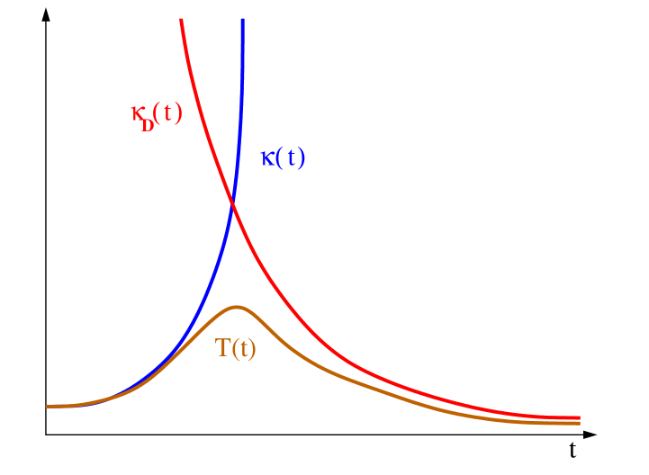
Figure 16: Possible behaviour of the evaporation temperature in an alternative semiclassical collapse and evaporation process based on critical configurations.

In this scenario the complete semiclassical geometry will have neither an apparent horizon nor an event horizon. In this circumstance there would be no trans-Planckian problem, nor information loss associated with the collapse and evaporation of this black hole-like object. Whether this scenario is viable or not will be the subject of future work.

Let us end by making a brief comment concerning modified dispersion relations. Everything we said in this paper assumes strict adherence to Lorentz symmetry. Even if semiclassical gravity contained Lorentz-violating traces in the form of modified dispersion relations at high energy, one would still expect that the resulting scenario for the collapse and evaporation of a black hole-like object would keep the quasi-stationary Hawking-like flux of particles as a robust prediction [24]. However, the complete conceptual scenario could be very different. In the presence of dispersion at high energies, the notion of horizon itself shows up only as a low-energy concept. For example, with superluminal modifications of the dispersion relations, high energy signals will be able to escape from the trapped region. The non-analytic behaviour of some sets of modes at the horizon become regularized. Therefore, the Stephens–’t Hooft–Whiting obstruction described above forbidding the formation of a (now approximate) trapping horizon need no longer apply. We expect that by analyzing different analogue models in which the Lorentz violating terms appear at different energy scales one would be able to explore the transition between all these alternative paradigms.

References

- [1] M. Novello, M. Visser and G. Volovik (eds.), Artificial Black Holes (Singapore, World Scientific, 2002).
- [2] C. Barceló, S. Liberati and M. Visser, “Analogue gravity,” Living Rev. Relativity 8, 12 (2005) [arXiv:gr-qc/0505065]. URL (cited on 22 March 2006): http://www.livingreviews.org/lrr-2005-12
- [3] C. Barceló, S. Liberati and M. Visser, “Analogue gravity from Bose-Einstein condensates,” Class. Quantum Grav. 18, 1137–1156 (2001) [arXiv:gr-qc/0011026].
- [4] M. Visser, C. Barceló and S. Liberati, “Analogue models of and for gravity,” Gen. Relativ. Gravit. 34, 1719–1734 (2002) [arXiv:gr-qc/0111111].
- [5] C. Barceló, S. Liberati, S. Sonego and M. Visser, “Causal structure of analogue spacetimes,” New J. Phys. 6, 186 (2004) [arXiv:gr-qc/0408022].
-
[6]
S. W. Hawking, “Black hole explosions,” Nature 248, 30–31 (1974);
——— “Particle creation by black holes,” Commun. Math. Phys. 43, 199–220 (1975); Erratum: ibid. 46, 206 (1976). - [7] N. D. Birrell and P. C. W. Davies, Quantum Fields in Curved Space (Cambridge, Cambridge University Press, 1982).
- [8] M. Visser, “Acoustic black holes: horizons, ergospheres, and Hawking radiation,” Class. Quantum Grav. 15, 1767–1791 (1998) [arXiv:gr-qc/9712010].
- [9] B. L. Hu, “Hawking-Unruh thermal radiance as relativistic exponential scaling of quantum noise,” in Thermal Field Theory and Applications, edited by Y. X. Gui, F. C. Khanna and Z. B. Su (Singapore, World Scientific, 1996), pp. 249–260 [arXiv:gr-qc/9606073].
- [10] M. Visser, “Essential and inessential features of Hawking radiation,” Int. J. Mod. Phys. D 12, 649–661 (2003) [arXiv:hep-th/0106111].
- [11] S. W. Hawking and G. F. R. Ellis, The Large Scale Structure of Space-Time (Cambridge, Cambridge University Press, 1973).
- [12] R. M. Wald, General Relativity (Chicago, University of Chicago Press, 1984).
- [13] S. Corley and T. Jacobson, “Black hole lasers,” Phys. Rev. D 59, 124011 (1999) [arXiv:hep-th/9806203].
- [14] R. Schützhold and W. G. Unruh, “Gravity wave analogues of black holes,” Phys. Rev. D 66, 044019 (2002).
- [15] S. Liberati, T. Rothman and S. Sonego, “Nonthermal nature of incipient extremal black holes,” Phys. Rev. D 62, 024005 (2000) [arXiv:gr-qc/0002019].
- [16] S. Liberati, T. Rothman and S. Sonego, “Extremal black holes and the limits of the third law,” Int. J. Mod. Phys. D 10, 33–39 (2001) [arXiv:gr-qc/0008018].
- [17] J. R. Oppenheimer and H. Snyder, “On continued gravitational contraction,” Phys. Rev. 56, 455–459 (1939).
-
[18]
P. Painlevé, “La mécanique classique et la theorie de la relativité,” C. R. Acad. Sci. (Paris) 173, 677–680 (1921).
A. Gullstrand, “Allgemeine Lösung des statischen Einkörperproblems in der Einsteinschen Gravitationstheorie,” Ark. Mat. Astron. Fys. 16, 1–15 (1922). - [19] L. Parker, “The production of elementary particles by strong gravitational fields,” in Asymptotic Structure of Space-Time, edited by F. P. Esposito and L. Witten (New York, Plenum, 1977), pp. 107–226.
- [20] G. E. Volovik, “Black-hole horizon and metric singularity at the brane separating two sliding superfluids,” Pisma Zh. Eksp. Teor. Fiz. 76, 296–300 (2002) [JETP Lett. 76, 240–244 (2002)] [arXiv:gr-qc/0208020].
- [21] D. G. Boulware, “Hawking radiation and thin shells,” Phys. Rev. D 13, 2169–2187 (1976).
- [22] A. Ashtekar and M. Bojowald, “Black hole evaporation: a paradigm,” Class. Quantum Grav. 22, 3349–3362 (2005) [arXiv:gr-qc/0504029].
- [23] C. R. Stephens, G. ’t Hooft and B. F. Whiting, “Black hole evaporation without information loss,” Class. Quantum Grav. 11, 621–647 (1994) [arXiv:gr-qc/9310006].
- [24] W. G. Unruh and R. Schützhold, “On the universality of the Hawking effect,” arXiv:gr-qc/0408009.