Stability of general relativistic static thick disks: the isotropic Schwarzschild thick disk

Abstract

We study the stability of general relativistic static thick disks, as an application we consider the thick disk generated by applying the “displace, cut, fill and reflect” method, usually known as the image method, to the Schwarzschild metric in isotropic coordinates. The isotropic Schwarzschild thick disk obtained from this method is the simplest model to describe, in the context of General Relativity, real thick galaxies. The stability under a general first order perturbation of the disk is investigated. The first order perturbation, when applying to the conservation equations, leads to a set of differential equations that are, in general, not self-consistent. This opens the possibility of performing various kinds of perturbations to transform the resulting system of equations into a self-consistent system. We perform a complete classification of the perturbations as well as the stability analysis for all the relevant physical perturbations. We found that, in general, the isotropic Schwarzschild thick disk is stable under these kinds of perturbations.

PACS: 04.40.Dg, 98.62.Hr, 04.20.Jb

I Introduction

Exact axial symmetric solutions of Einstein field equations are a good starting point for modeling astrophysical applications in General Relativity. This is due to the fact that the natural shape of an isolated self-gravitating fluid is axially symmetric. In the last decades, several exact solutions were studied as possible galactic models. Static thin disk solutions were first studied by Bonnor and Sackfield bon:sac and Morgan and Morgan mor:mor1 , where they considered disks without radial pressure. Disks with radial pressure and with radial tension have been considered by Morgan and Morgan mor:mor2 and González and Letelier gon:let1 , respectively. Self-similar static disks were studied by Lynden-Bell and Pineault lyn:pin , and Lemos lem . Moreover, solutions that involve superpositions of black holes with static disks were analyzed by Lemos and Letelier lem:let1 ; lem:let2 ; lem:let3 and Klein kle1 . Also, relativistic counter-rotating thin disks as sources of the Kerr type metrics were found by Bičák and Ledvinka bic:led . Counter-rotating models with radial pressure and dust disks without radial pressure were studied by González and Espitia gon:esp , and García and González gar:gon , respectively; while rotating disks with heat flow were studied by González and Letelier gon:let2 . Furthermore, static thin disks as sources of known vacuum spacetimes from the Chazy-Curzon metric cha ; cur and Zipoy-Voorhees zip ; voo metric were obtained by Bičák, Lynden-Bell and Katz bic:lyn1 . Also, Bičák, Lynden-Bell and Pichon bic:lyn2 found an infinite number of new static solutions. Stationary disk models including electric fields led:zof , magnetic fields let , and both electric and magnetic fields kat:bic have been studied. In the last years, exact solutions for thin disks made with single and composite halos of matter vog:let1 , charged dust vog:let2 and charged perfect fluid vog:let3 were obtained. For a survey on relativistic gravitating disks, see sem ; kar:hur . Most of the models constructed above were found using the metric to calculate its energy momentum-tensor, i.e. a inverse problem. Several exact disk solutions were found using the direct method that consists in computing the metric for a given energy momentum tensor representing the disk neu:mei ; kle:ric ; kle2 ; fra:kle ; kle3 ; kle4 ; kle5 . In a first approximation, the galaxies can be thought to be thin, this usually simplifies the analysis and provides very useful information. But, in order to model real physical galaxies the thickness of the disks must be considered. Exact axially symmetric relativistic thick disks in different coordinate systems were studied by González and Letelier gon:let3 . Also, different thick disks were obtained from the Schwarzschild metric in different coordinates systems with the “displace, cut, fill, and reflect” method vog:let4 . Recently, a relativistic generalization of the Miyamoto-Nagai potential was obtained vog:let5 .

The applicability of these disks models to any structure found in Nature lays in its stability. The study of the stability, analytically or numerically, is vital to the acceptance of the particular model. Also, the study of different types of perturbations, when applied to these models, might give an insight on the formation of bars, rings or different stellar patterns. Furthermore, a perturbation can cause the collapse of a stable object with the posterior appearance of a different kind of structure. An analytical treatment of the stability of disks in Newtonian theory can be found in bin:tre ; fri:pol and references therein. In general, the stability of disks in General Relativity is done in two ways. One way is to study the stability of the particle orbits along geodesics. This kind of studied was made by Letelier let2 transforming the Rayleigh criterion of stability ray ; lan:lif into a general relativistic formulation. Using this criterion, the stability of orbits around black holes surrounded by disks, rings and multipolar fields were analyzed let2 . Also, this criterion was employed in vog:let1 to study the stability of the isotropic Schwarzschild thin disk, and thin disks of single and composite halos. The stability of circular orbits in stationary axisymmetric spacetimes are studied in bar ; abr:pra . Moreover, the stability of circular orbits of the Lemos-Letelier solution lem:let2 for the superposition of a black hole and a flat ring are considered in sem:zac ; sem:zac2 ; sem2 . Also, Bičák, Lynden-Bell and Katz bic:lyn1 analyzed the stability of several thin disks without radial pressure or tension studying their velocity curves and specific angular momentum. The other way to study the stability of disks is to perturb its energy momentum tensor. This way is more complete than the analysis of particle motions along geodesics because we are taking into account the collective behavior of the particles. However, there are few studies in the literature performing this kind of perturbation. A general stability study of a relativistic fluid, with both bulk and dynamical viscosity, was done by Seguin seg . He considered the coefficients of the perturbed variables as constants, i.e. local perturbations. Usually, this condition is too restrictive. Stability analysis of thin disks from the Schwarzschild metric, the Chazy-Curzon metric and Zipoy-Voorhees metric perturbing their energy momentum tensor with a general first order perturbation were made by Ujevic and Letelier uje:let , finding that the thin disks without radial pressure are not stable uje:let2 .

In order to have a general relativistic physical model for galaxies, we must considered, first of all, the thickness of the disk and its stability under perturbations of the fluid quantities. The purpose of this work is to study numerically the stability of the isotropic Schwarzschild thick disk under a general first order perturbation. The perturbation is done in the temporal, radial, axial and azimuthal components of the quantities involved in the energy momentum tensor of the fluid. In the general thick disk case, the perturbed conservation equations are not self-consistent because the number of unknowns is larger than the number of equations. In order to make the system of equation self-consistent we must chose a combination of the perturbed quantities. This opens the possibility to perform several types of perturbed quantities combinations that provide a self-consistent set of equations. In this manuscript, we study the physical accepted perturbations. We mean by a physical perturbation the fact that a perturbation in a given direction of the pressure must create a perturbation in the same direction of the four velocity. The energy momentum perturbation considered in this manuscript is treated as “test matter”, so it does not modified the background metric obtained from the solution of Einstein equations.

The article is organized as follows. In Sec. II, we present the general perturbed conservation equations for the thick disk case. The energy momentum tensor is considered diagonal with its elements different from zero. Also, the energy momentum perturbation is considered as “test matter”. In this section we classified the possible perturbed quantities combinations that leads to a self-consistent set of the perturbed conservation equations of motion. In Sec. III, we present the thick disk considered for the analysis, i.e. the isotropic Schwarzschild thick disk. The form of its energy density and pressures, as well as, the restrictions that the thermodynamic quantities must obey to satisfy the strong, weak and dominant energy conditions are shown. Later, in Sec. IV, we perform all the physical accepted perturbations to the isotropic Schwarzschild thick disk to study its stability. Finally, in Sec. V, we summarized our results.

II Perturbed Equations

The thick disk considered is a particular case of the general static, axially symmetric metric

$$ds^{2}=-e^{2\Psi_{1}}dt^{2}+e^{2\Psi_{2}}R^{2}d\theta^{2}+e^{2\Psi_{3}}(dR^{2}+dz^{2}),$$ (1)

where $\Psi_{1}$, $\Psi_{2}$ and $\Psi_{3}$ are functions of the variables ($R,z$). (Our conventions are: $G=c=1$. Metric signature +2. Partial and covariant derivatives with respect to the coordinate $x^{\mu}$ denoted by $,\mu$ and $;\mu$, respectively.)

In its rest frame, the energy momentum tensor of the fluid $T^{\mu\nu}$ is diagonal with components (-$\rho,p_{R},p_{\theta},p_{z}$), where $\rho$ is the energy density and ($p_{R},p_{\theta},p_{z}$) are the radial, azimuthal and axial pressures or tensions, respectively. So, in this frame of reference, the energy momentum tensor can be written as

$$T^{\mu\nu}=\rho U^{\mu}U^{\nu}+p_{R}X^{\mu}X^{\nu}+p_{\theta}Y^{\mu}Y^{\nu}+p_{z}Z^{\mu}Z^{\nu},$$ (2)

where $U^{\mu}$, $X^{\mu}$, $Y^{\mu}$, and $Z^{\mu}$ are the four vectors of the orthonormal tetrad

$$U^{\mu}=e^{-\Psi_{1}}(1,0,0,0),$$

$$X^{\mu}=e^{-\Psi_{3}}(0,1,0,0),$$

$$Y^{\mu}=\frac{e^{-\Psi_{2}}}{R}(0,0,1,0),$$

$$X^{\mu}=e^{-\Psi_{3}}(0,0,0,1),$$ (3)

which satisfy the orthonormal relations. Note that with the above definitions, the timelike four velocity of the fluid is $U^{\mu}$ and the quantities $X^{\mu}$, $Y^{\mu}$, and $Z^{\mu}$ are the spacelike principal directions of the fluid. Furthermore, the energy momentum tensor satisfies Einstein field equations, $G_{\mu\nu}=\kappa T_{\mu\nu}$.

Due to the form of our axially symmetric metric, the quantities involved in the energy momentum tensor and the coefficients of the perturbed conservation equations are functions of the coordinates ($R,z$) only. Let us consider a general perturbation $A^{\mu}_{P}$ of a quantity $A^{\mu}$ in the form

$$A^{\mu}_{P}(t,R,\theta,z)=A^{\mu}(R,z)+\delta A^{\mu}(t,R,\theta,z),$$ (4)

where $A^{\mu}(R,z)$ is the unperturbed quantity and $\delta A^{\mu}(t,R,\theta,z)$ is the perturbation. Replacing (4) for each quantity in the energy momentum tensor (2) and reordering terms, we obtain that

$$T^{\mu\nu}_{P}(t,R,\theta,z)=T^{\mu\nu}(R,z)+\delta T^{\mu\nu}(t,R,\theta,z).$$ (5)

Hereafter, we assume that the perturbed energy momentum tensor does not modify the background metric found by solving the Einstein field equation $G_{\mu\nu}=\kappa T_{\mu\nu}$. In other words, the perturbation $\delta T^{\mu\nu}$ is treated as a test fluid. Not considering the fluid as a test fluid is a second degree of approximation to the stability problem in which the emission of gravitational radiation is considered. With the perturbed energy momentum tensor $T^{\mu\nu}_{P}$ and Einstein field equations, we obtain that the perturbed energy momentum equations for the problem must obey

$$\delta T^{\mu\nu}_{;\nu}=0.$$ (6)

These four equations can be found in Ref. uje:let from Eq. (8II) to Eq. (13II). Hereafter, the equations from Ref. uje:let will be denoted by II. In this manuscript we are interested in linear perturbations of the energy momentum tensor. So, in writing the explicit form of the four equations (6) we discard terms of order greater or equal to ($\delta^{2}$). It is explained in uje:let , that if we want a consistent perturbation model the tetrad must be perturbed. Moreover, demanding the orthonormal condition for the perturbed tetrad we find several relations between their components (14II). Because of the form of the perturbed energy momentum equation for the axially symmetric metric (1), the connection coefficients are only functions of the coordinates ($R,z$). Therefore, all the coefficients on the perturbed conservation equations depend only on ($R,z$) and we can construct a general perturbation of the form

$$\delta A^{\mu}(t,R,\theta,z)=\delta A^{\mu}(R,z)e^{i(k_{\theta}\theta-wt)}.$$ (7)

Hereafter $\delta A^{\mu}\equiv\delta A^{\mu}(R,z)$. In this article, we are interested in perturbations of the four velocity $U^{\mu}$ and the thermodynamics variables ($\rho,p_{R},p_{\theta},p_{z}$). For that reason, we see in (14II) that the $t$ components of the tetrad $\delta X^{t}$, $\delta Y^{t}$ and $\delta Z^{t}$ must be perturbed. Moreover, the tetrad perturbations $\delta X^{\theta}$, $\delta X^{z}$ and $\delta Y^{z}$ are not related whatsoever to the four-velocity or the thermodynamic variables perturbations and we can set them equal to zero. With these assumptions, the perturbation (7) and conditions (14II), the general perturbed energy momentum equations (8II)-(13II) can be cast into the particular form

$\mu=t$

$$\delta U^{R}_{,R}(\rho U^{t}+\xi_{1}p_{R}X^{R})+\delta U^{z}_{,z}(\rho U^{t}+\xi_{3}p_{z}Z^{z})+\delta U^{R}[{\rm F}(t,R,\rho U^{t})+\xi_{1,R}p_{R}X^{R}+\xi_{1}{\rm F}(t,R,p_{R}X^{R})]$$

$$+\delta U^{\theta}[ik_{\theta}(\rho U^{t}+\xi_{2}p_{\theta}Y^{\theta})]+\delta U^{z}[{\rm F}(t,z,\rho U^{t})+\xi_{3,z}p_{z}Z^{z}+\xi_{3}{\rm F}(t,z,p_{z}Z^{z})]+\delta\rho(-iwU^{t}U^{t})=0,$$ (8)

$\mu=R$

$$\delta p_{R,R}(X^{R}X^{R})+\delta U^{R}[-iw(\rho U^{t}+\xi_{1}p_{R}X^{R})]+\delta\rho(U^{t}U^{t}\Gamma^{R}_{tt})$$

$$+\delta p_{R}{\rm G}(R,R,X^{R}X^{R})+\delta p_{\theta}(Y^{\theta}Y^{\theta}\Gamma^{R}_{\theta\theta})+\delta p_{z}(Z^{z}Z^{z}\Gamma^{R}_{zz})=0,$$ (9)

$\mu=\theta$

$$\delta U^{\theta}[-w(\rho U^{t}+\xi_{2}p_{\theta}Y^{\theta})]+\delta p_{\theta}(k_{\theta}Y^{\theta}Y^{\theta})=0,$$ (10)

$\mu=z$

$$\delta p_{z,z}(Z^{z}Z^{z})+\delta U^{z}[-iw(\rho U^{t}+\xi_{3}p_{z}Z^{z})]+\delta\rho(U^{t}U^{t}\Gamma^{z}_{tt})$$

$$+\delta p_{R}(X^{R}X^{R}\Gamma^{z}_{RR})+\delta p_{\theta}(Y^{\theta}Y^{\theta}\Gamma^{z}_{\theta\theta})+\delta p_{z}{\rm G}(z,z,Z^{z}Z^{z})=0.$$ (11)

where

$${\rm F}(I,J,K)=K_{,J}+K(2\Gamma^{I}_{IJ}+\Gamma^{\alpha}_{\alpha J}),$$ (12)

$${\rm G}(I,J,K)=K_{,J}+K(\Gamma^{I}_{IJ}+\Gamma^{\alpha}_{\alpha J}),$$ (13)

and $\Gamma^{\alpha}_{\beta\gamma}$ are the Christoffel symbols.

Besides the four equations furnished by the energy momentum conservation equations, $T^{\mu\nu}_{;\nu}=0$, there is another important conservation equation, the equation of continuity,

$$(nU^{\mu})_{;\mu}=0,$$ (14)

where $n$ is the proper number density of particles. The proper number density of particles $n$, and the total energy density $\rho$ are related through the relation,

$$\rho=nm_{b}+\varepsilon,$$ (15)

where $m_{b}$ is the constant mean baryon mass and $\varepsilon$ the internal energy density. Multiplying Eq. (15) by $U^{\mu}$, performing the covariant derivative ($;\mu$) and using Eq. (14), we obtain that

$$(\rho U^{\mu})_{;\mu}=(\varepsilon U^{\mu})_{;\mu}.$$ (16)

Now, from the relation $U_{\nu}T^{\mu\nu}_{;\mu}=0$ and the energy momentum tensor (2), we obtain and expression for $(\rho U^{\mu})_{;\mu}$. Substituting this last expression into Eq. (16) we finally arrive at

$$(\varepsilon U^{\mu})_{;\mu}=p_{R}X^{\mu}U_{\nu}X^{\nu}_{;\mu}+p_{\theta}Y^{\mu}U_{\nu}Y^{\nu}_{;\mu}+p_{z}Z^{\mu}U_{\nu}Z^{\nu}_{;\mu},$$ (17)

which is a first order differential equation for $\varepsilon$. Therefore, with $\varepsilon$ given by (17) the equation of continuity (14) is satisfied. For this reason, the continuity equation can be omitted for our stability analysis because, in principle, we can always find a solution for $\varepsilon$. Hereafter, the contribution of $nm_{b}$ and $\varepsilon$ to the total energy density are consider in $\rho$. In the case when the internal energy density of the fluid is given, the equation of continuity must be considered. In other words, the knowledge of the thermodynamic properties of the disk is important for actual applications. The thermodynamic properties of the system can be obtained from observations or theoretically from the Fokker-Planck equation, where we obtain the particle distribution function of the disk. Solving the Fokker-Planck equation is not an easy task, but some progress in Newtonian gravity have been done (uje:let3, ).

The four equations (II-II) contain seven independent unknowns, say $\delta U^{R},\delta U^{\theta},\delta U^{z},\delta\rho,\delta p_{R},\delta p_{\theta},\delta p_{z}$. So, at this point, the number of unknowns are greater than the number of equations and the system is not self-consistent. This opens the possibility to perform different kind of perturbations to make the system self-consistent. In Table 1 we present the classification for all the possible perturbations that lead to a self-consistent system of equations. We divided the table in three sections that depend on the number of perturbed quantities, i.e. two, three and four quantities perturbations. Equation (10) is important for this classification because it only involve the two unknowns ($\delta U^{\theta},p_{\theta}$). Therefore, if one of them is, by construction, equal to zero then the other unknown is also zero. There is a possibility to avoid the other unknown to be equal zero, i.e. if the unknown coefficient is equal zero. This situation can occur in particular space-time points. We do not consider these cases. The system of equations for the different combinations of the perturbed quantities reduce to various differential equations, the form of the particular differential equation is written in the column Differential Equation. We denote by ODE# and PDE# an ordinary different equation of order # and a partial differential equation of order #, respectively. The differential equation marked with a question mark (?) means that other four perturbations, that do not include the $\delta U^{\theta}$ and $\delta p_{\theta}$ perturbations, are not self-consistent, but they might be if we assume other imposed conditions for the involve quantities, as for example $\delta p_{R}\equiv\delta p_{z}$. Moreover, if we assume other imposed conditions for the different types of perturbation shown in Table 1, the differential equation classification may change.

We are interested in consistent physical perturbations. For that reason we search for perturbations in which the velocity perturbation in a certain direction leads to a pressure perturbation in the same direction. For example, if we perturbed the $z$ component of the velocity $\delta U^{z}$ then we must perturb $\delta p_{z}$ to have a consistent physical problem. With the above criterion only four perturbations are allowed, these are marked with (*) in Table 1. These perturbations will be considered in our thick disk model. Furthermore, we perform the perturbation $\delta U^{R},\delta p_{R},\delta U^{z},\delta p_{z}$ with the extra imposed condition $\delta p_{R}\equiv\delta p_{z}$. This last perturbation are among the ones denoted by question mark. In this particular case, the system of equations reduced to a second order partial differential equation.

Table 1: Differential equation classification for all the possible different types of perturbations. The perturbations marked with (*) are the ones that are physical accepted. Other physical accepted perturbations are marked with (?) but these perturbations require extra imposed conditions.

Perturbations				Differential Equation
Two Perturbations
		$\delta p_{R}$	$\delta p_{z}$	PDE2
Three Perturbations
	$\delta U^{R}$	$\delta p_{R}$	$\delta U^{z}$	PDE2
	$\delta U^{R}$	$\delta p_{R}$	$\delta p_{z}$	ODE1 + PDE2
	$\delta U^{R}$	$\delta p_{R}$	$\delta\rho$	ODE2 *
	$\delta U^{R}$	$\delta U^{z}$	$\delta p_{z}$	PDE2
	$\delta U^{R}$	$\delta U^{z}$	$\delta\rho$	PDE1
	$\delta U^{R}$	$\delta p_{z}$	$\delta\rho$	PDE2
	$\delta p_{R}$	$\delta U^{z}$	$\delta p_{z}$	ODE1 + PDE2
	$\delta p_{R}$	$\delta U^{z}$	$\delta\rho$	PDE2
	$\delta U^{z}$	$\delta p_{z}$	$\delta\rho$	ODE2 *
Four Perturbations
$\delta U^{\theta}$	$\delta p_{\theta}$	$\delta U^{R}$	$\delta p_{R}$	ODE2 *
$\delta U^{\theta}$	$\delta p_{\theta}$	$\delta U^{R}$	$\delta U^{z}$	PDE1
$\delta U^{\theta}$	$\delta p_{\theta}$	$\delta U^{R}$	$\delta p_{z}$	PDE2
$\delta U^{\theta}$	$\delta p_{\theta}$	$\delta U^{R}$	$\delta\rho$	ODE1
$\delta U^{\theta}$	$\delta p_{\theta}$	$\delta U^{z}$	$\delta p_{z}$	ODE2 *
$\delta U^{\theta}$	$\delta p_{\theta}$	$\delta U^{z}$	$\delta p_{R}$	PDE2
$\delta U^{\theta}$	$\delta p_{\theta}$	$\delta U^{z}$	$\delta\rho$	ODE1
$\delta U^{\theta}$	$\delta p_{\theta}$	$\delta p_{R}$	$\delta\rho$	ODE1
$\delta U^{\theta}$	$\delta p_{\theta}$	$\delta p_{z}$	$\delta\rho$	ODE1
Without $\delta U^{\theta}$, $\delta p_{\theta}$				?

III Isotropic Schwarzschild Thick Disk

The static isotropic Schwarzschild thick disk was found in vog:let4 by applying the displace, cut, fill and replace method to the axially symmetric metric (1) with the definitions

$$\Psi_{1}=\ln\left(\frac{2r-m}{2r+m}\right),$$ (18)

$$\Psi_{2}=\Psi_{3}=2\ln\left(1+\frac{m}{2r}\right),$$ (19)

where $r^{2}=R^{2}+(h+b)^{2}$, ($m>0$, $b>0$) are parameters, and $h$ is a function of the coordinate $z$ given by

$$h(z)=\left\{\begin{tabular}[]{ll}$-z+C,$&$z\leq-a,$\\ $Az^{2}+Bz^{2n+2}$,&$-a\leq z\leq a,$\\ $z+C,$&$z\geq a,$\end{tabular}\right.$$ (20)

with

$$A=\frac{2n+1-ac}{4na},$$

$$B=\frac{ac-1}{4n(n+1)a^{2n+1}},$$

$$C=-\frac{a(2n+1+ac)}{4(n+1)},$$

where $n=1,2,\cdots$, and $c$ is the jump of the second derivative on $z=\pm a$, see vog:let4 . The energy density and the different pressures for this thick disk are

$$\rho=\frac{64m}{(m+2r)^{5}}[3(h+b)^{2}(1-h^{\prime 2})$$

$$\hskip 85.35826pt+r^{2}[h^{\prime 2}-1+h^{\prime\prime}(h+b)]],$$ (21)

$$p_{R}=p_{\theta}=\frac{32m^{2}}{(m+2r)^{5}(-m+2r)}[2(h+b)^{2}(1-h^{\prime 2})$$

$$\hskip 85.35826pt+r^{2}[h^{\prime 2}-1+h^{\prime\prime}(h+b)]],$$ (22)

$$p_{z}=\frac{64m^{2}(1-h^{\prime 2})(h+b)^{2}}{(m+2r)^{5}(-m+2r)},$$ (23)

where the prime ($\prime$) represents derivative with respect to the axial coordinate $z$. We have set in Eqs. (21)-(23), without losing generalization, the range of the $z$ coordinate between $-1\leq z\leq 1$. These means that the parameter $a$ of vog:let4 is equal to one. To satisfy the strong energy condition we must have that $\epsilon=\rho+p_{R}+p_{\theta}+p_{z}\geq 0$, the weak energy condition requires $\rho\geq 0$ and the dominant energy condition requires $|p_{R}/\rho|\leq 1$, $|p_{\theta}/\rho|\leq 1$ and $|p_{z}/\sigma|\leq 1$. If we set the parameters ($m,b,n,c$) explained in vog:let4 equal to ($m=1,b=2,n=1,c=0$), we obtain a thick disk with all energy conditions satisfied. Also, the level curves for this disk show that it is physically acceptable. For this set of parameters, the function $h$ has the form $h=3/4z^{2}-1/8z^{4}$. We remark that these are not the only parameters in which the level curves are physically accepted. In the next section we applied the selected perturbations of Sec. II to the isotropic Schwarzschild thick disk mention above and studied its stability.

IV Perturbations

Before we start applying the different kinds of perturbations to the isotropic Schwarzschild thick disk we must have some considerations. Note that the exact thick disk metric considered is infinite in the radial direction, but finite in the $z$ direction. In order to study the stability we need a criterion to make a finite disk, i.e. we need a cutoff in the radial coordinate. In Eqs. (21), (22) and (23), we see that the thermodynamic quantities decrease rapidly enough to define a cutoff radius. The cutoff radius $R_{cut}$ is set by the following criterion: the energy density within the thick disk formed by the cutoff radius is more than 90% of the infinite thick disk energy density. This leads to a cutoff radius of $R_{cut}=20$ units. Furthermore, the other 10% of the energy density that is distributed from outside the cutoff radius to infinity can be treated, if necessary, as a perturbation in the outermost boundary condition.

IV.1 Perturbation with $\delta U^{\theta}$, $\delta p_{\theta}$, $\delta U^{R}$, $\delta p_{R}$

We start perturbing the four velocity in its components $\theta$ and $R$, from the physical considerations mentioned in Sec. II we also expect variations in the thermodynamic quantities $p_{\theta}$ and $p_{R}$. The set of equations (II)-(II) reduce to a second order ordinary differential equation for the perturbation $\delta p_{R}$, say

$$F_{A}{\delta p_{R}}_{,RR}+F_{B}{\delta p_{R}}_{,R}+F_{C}\delta p_{R}=0,$$ (24)

where $(F_{A},F_{B},F_{C})$ are functions of ($R,z,w,k_{\theta}$), see Appendix A. For this particular case we have for the perturbation, $\delta p_{\theta}=-\delta p_{R}$.

Note that in Eq. (24) the coordinate $z$ only enters like a parameter. Moreover, the equation for $\delta p_{R}$ is independent of the parameter $w$, but $w$ needs to be different from zero to reach that form. The second order equation (24) is solved numerically with two boundary conditions, one at $R\approx 0$ and the other at the cutoff radius. At $R\approx 0$ we set the perturbation $\delta p_{R}$ to be $\approx$ 10% of the unperturbed pressure $p_{R}$ (22). In the outer radius of the disk we set $\delta{p_{R}}|_{R=R_{cut}}=0$ because we want our perturbation to vanish when approaching the edge of the disk, and in that way, to be in accordance with the linear perturbation applied. We say that our perturbations are valid if their values are lower, or of the same order of magnitude, than the 10% values of the unperturbed quantities.

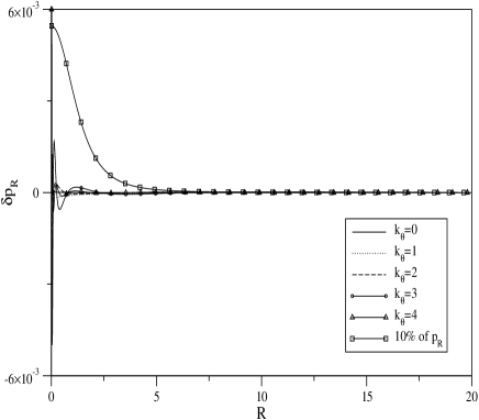
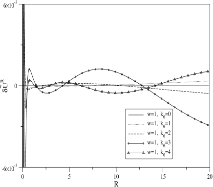
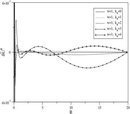
Figure 1: Profiles of the amplitude perturbations modes for the radial pressure, radial physical velocity and azimuthal physical velocity for the case when $z=0$, $w=1$ and $k_{\theta}=0,1,2,3,4$. In the pressure perturbation graph the 10% profile value of the radial pressure is depicted to ensure that the perturbations are in accordance with the stability criterion imposed. The value of the velocity perturbation profiles are well below the particles escape velocity.

In Fig. 1, we present the amplitude profile of the radial pressure perturbation, the physical radial velocity perturbation $\tilde{\delta U^{R}}=\sqrt{g_{RR}}\delta U^{R}$ and the physical azimuthal velocity perturbation $\tilde{\delta U^{\theta}}=\sqrt{g_{\theta\theta}}\delta U^{\theta}$ in the plane $z=0$. In Fig. 1 we see that the perturbation $\delta p_{R}$ decreases rapidly with $R$ and has oscillatory behavior. At first sight, the perturbation $\delta p_{R}$ appears to be stable for all $R$, but in order to make a complete analysis we have to compare at each radius the values of the different perturbations with the values of the radial pressure. For this purpose, we included in the same graph a profile of the 10% value of $p_{R}$. We see that the perturbations of $\delta p_{R}$ for different values of $k_{\theta}$ are always lower or, at least, of the same order of magnitude when compared to these 10% values.

Our four velocity $U^{\mu}$ (3) has only components in the temporal part, so we do not have values of $U^{R}$ and $U^{\theta}$ to make comparisons with the perturbed values $\tilde{\delta U^{R}}$ and $\tilde{\delta U^{\theta}}$ of Fig 1. For that reason we compared, in first approximation, the amplitude profiles of these perturbations with the value of the escape velocity in the Newtonian limit. In the Newtonian limit of General Relativity, we have the well known relation $g_{00}=\eta_{00}+2\Phi$. So, the Newtonian escape velocity $V_{e}=\sqrt{2|\Phi|}$ can be written as

$$V_{e}=\left(1-\frac{(1-\frac{m}{2r})^{2}}{(1+\frac{m}{2r})^{2}}\right)^{1/2}.$$ (25)

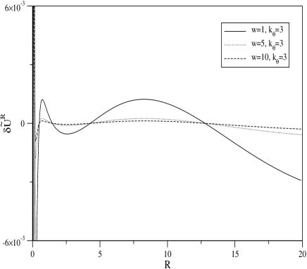
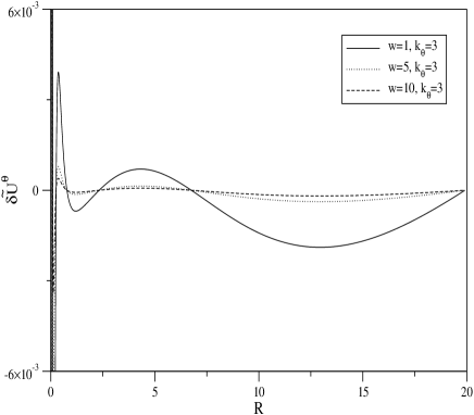
Figure 2: Profiles of the amplitude perturbations modes for the radial physical velocity and the azimuthal velocity for the case when $z=0$, $k_{\theta}=3$ and $w=1,5,10$. We note that when we increase the value of the frequency $w$ the modes are more stable.

For the parameters considered, we have that at $(R=0,z=0)$ and $(R=20,z=0)$ the escape velocity is $V_{e}=0.8$ and $V_{e}\approx 0.31$, respectively. The escape velocity values have a small variation with $z$. So, with this criterion, we may say that the perturbations $\tilde{\delta U^{R}}$ and $\tilde{\delta U^{\theta}}$ are stable because their values are always well below the escape velocity value. Recall that the perturbation $\delta p_{R}$ does not depend on the parameter $w$, but the perturbations $\tilde{\delta U^{R}}$ and $\tilde{\delta U^{\theta}}$ do. In Fig. 2 we show the numerical solution of $\tilde{\delta U^{R}}$ and $\tilde{\delta U^{\theta}}$ for different values of the frequency $w$ with the same wavenumber $k_{\theta}$. We see that when we increase the value of the parameter $w$ the perturbations become more stable. This behavior is the same for other values of $k_{\theta}$.

In this subsection we set the value of the parameter $z=0$. We performed the same analysis for different values of the parameter $-1<z<1$, and we found that the perturbations show the same qualitative behavior. Therefore, we can said that the isotropic thick disk is stable under perturbations of the form presented in this subsection. Nevertheless, if we treat the 10% of the energy density as a perturbation in the outermost radius of the disk by setting $\delta p_{R}|_{R=R_{cut}}=\epsilon$, where $\epsilon<10\%$ of $p_{R}|_{R=R_{cut}}$ the qualitative behavior of the mode profiles are the same. From these results, we can say that the general linear perturbation applied is stable, and for that reason, the perturbations do not form more complex structures like rings, bars or halos. Moreover, if we set the frequency $w\rightarrow iw$ we obtain the same equation for the perturbation $\delta p_{R}$, say (24). In this case, the real part of the general perturbation (7) diverge with time and the perturbation is not stable. These last considerations can be applied to every perturbation in the following subsections.

IV.2 Perturbation with $\delta U^{\theta}$, $\delta p_{\theta}$, $\delta U^{z}$, $\delta p_{z}$

In this subsection we perturb the four velocity in its components $\theta$ and $z$, and we expect variations in the thermodynamic quantities $p_{\theta}$ and $p_{z}$. The set of equations (II)-(II) reduce to a second order ordinary differential equation for the perturbation $\delta p_{z}$ given by

$$F_{A}{\delta p_{z}}_{,zz}+F_{B}{\delta p_{z}}_{,z}+F_{C}\delta p_{z}=0,$$ (26)

where $(F_{A},F_{B},F_{C})$ are functions of ($R,z,w,k_{\theta}$), see Appendix B. Note that in Eq. (26) the coordinate $R$ only enters like a parameter. Like the previous case, Eq. (26) is independent of the parameter $w$, but in order to reach that form we must have $w$ different from zero. The second order equation (26) is solved numerically with two boundary conditions, one in $z=0$ and the other in $z=1$. At $z=0$ we set the perturbation $\delta p_{z}$ to be $\approx 10\%$ of the unperturbed pressure $p_{z}$ (23). In the outer plane of the disk we set $\delta p_{z}|_{z=1}=0$ because we want our perturbation to vanish when approaching the edge of the disk, and in that way, to be in accordance with the linear perturbation applied.

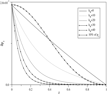
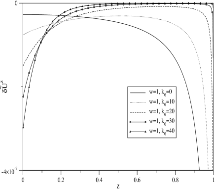
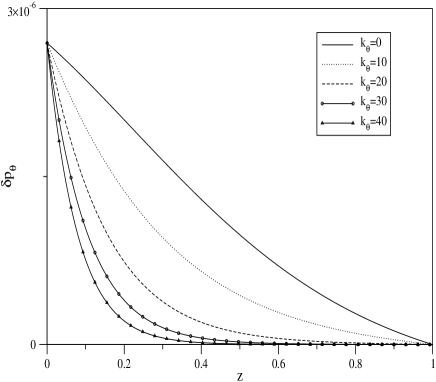
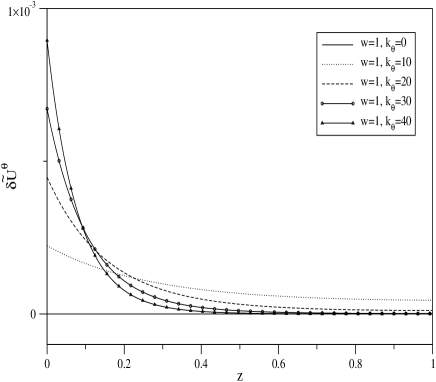
Figure 3: Profiles of the amplitude perturbations modes for the axial pressure, azimuthal pressure, axial physical velocity and azimuthal physical velocity for the case when $R=0.1$, $w=1$ and $k_{\theta}=0,10,20,30,40$. In the pressure perturbation graph the 10% profile value of the axial pressure is depicted to ensure that the perturbations are in accordance with the stability criterion imposed. In the azimuthal pressure perturbation graph the 10% profile was omitted because the values are three order of magnitudes higher. The values of the azimuthal velocity perturbation profiles are well below the particles escape velocity and the modes are stable. For the axial velocity perturbation profiles we see that the geometric properties of the disk create a kind of wall that impedes the particles for going out.

In Fig 3, we present the amplitude profiles of the axial pressure perturbation, the azimuthal pressure perturbation, the physical axial velocity $\tilde{\delta U^{z}}=\sqrt{g_{zz}}\delta U^{z}$ and the physical azimuthal velocity for the value of the parameter $R=0.1$. For comparison reasons, we included in the graph of the axial pressure perturbation the amplitude profile that corresponds to 10% of the value of $p_{z}$. We see in this graph that the modes profiles of the axial pressure are below, or of the same order of magnitude, when compared to the 10% profile. In this example the modes with wavenumber $k_{\theta}=0$ and $k_{\theta}=10$ have within the disk regions in which the profile values exceed the 10% profile. This perturbations are near the validity criterion used for the perturbations. In the axial velocity perturbations graph we see that the profiles suffer a sudden variation near the edge of the disk $z=1$. The axial velocity perturbation tends to expel the particles out from the disk. In our case, the particles are not allow to escape from the disk due to the fact that our geometrical disk is only valid for $-1\leq z\leq 1$. For that reason, the particles feel a kind of a wall that impedes them from going out. It is clear from the axial velocity perturbation profiles that the two nodes $(w=1,k_{\theta}=0)$ and $(w=1,k_{\theta}=10)$ are not stable, while the rest of the nodes are stable if we discard the region that is near the edge of the disk at $z=1$. Note that the starting point of the sudden variation of the axial velocity perturbation coincides with the radius in which the axial pressure perturbation exceeds the 10% value profile of $p_{z}$. Also, in Fig. 3, we see that the azimuthal pressure perturbations and the azimuthal velocity perturbations for different modes are stable. In the case of the azimuthal pressure, we have not included the 10% profile because is three order of magnitude higher than the perturbation value. Note that the amplitude values of azimuthal velocity perturbation are below the escape velocity considered for the disk.

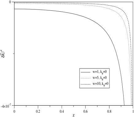
Figure 4: Profiles of the amplitude perturbations modes for the axial physical velocity for the case when $R=0.1$, $k_{\theta}=0$ and $w=1,5,10$. We note that if we increase the value of the $w$ parameter, the region in which the mode is stable increases. For higher values of $w$ the modes are stable if we discard the region near $z=1$.

The perturbation $\delta p_{z}$ does not depend on the parameter $w$, but the perturbations $\tilde{\delta U^{z}}$ and $\tilde{\delta U^{\theta}}$ do depend. In Fig. 4, we show the profile for the mode $k_{\theta}=0$ with different values of the frequency $w$ for the perturbation $\tilde{\delta U^{z}}$. We see that when we increase the value of the parameter $w=1$, the velocity perturbations are more stable (if we neglect the region near the edge of the disk at $z=1$). This is due to the fact that the frequency $w$ only enters the equation for $\delta U^{z}$ like a scale factor.

We have performed the same above analysis for different values of the parameter $R$, and we found that the qualitative behavior is the same. With these results we can say, if we neglect the region near the edge of the disk at $z=1$, that the isotropic thick disk is always stable for higher values of the parameter $w$ and has some stable modes for lower values of $w$. Moreover, for lower values of the frequency $w$, some modes of our general first order perturbation are not stable. In these cases, more complex structures may be form, but in order to study them, we need a higher order perturbation formalism.

IV.3 Perturbation with $\delta U^{R}$, $\delta p_{R}$, $\delta\rho$

In this subsection, we perturb the radial component of the four velocity, the radial pressure and the energy density of the fluid. The set of equations (II)-(II) reduce to a second order ordinary differential equation for the perturbation $\delta p_{R}$ of the form (24). The form of the functions $(F_{A},F_{B},F_{C})$ are given in Appendix C. In this case, the coordinate $z$ only enters like a parameter. Due to the fact that we are not considering perturbations in the azimuthal axis, the coefficients of the second order ordinary diffetential equation do not depend on the wavenumber $k_{\theta}$. This second order equation is solved numerically with the same boundary conditions described in Sec. IV-A.

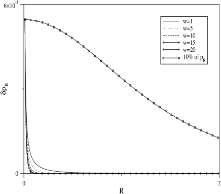
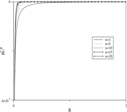
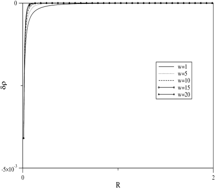
Figure 5: Profiles of the amplitude perturbations modes for the radial pressure, radial physical velocity and energy density for the case when $z=0$ and $w=1,5,10,15,20$. As in Fig. 1, we have depicted the 10% profile value of the radial pressure in the pressure perturbation graph. We see from these graphs that the pressure perturbation values are well below the 10% profile. In the energy density perturbation graph the 10% profile of the energy density was omitted because the values are two order of magnitudes higher. Also, the values of the velocity perturbations profiles are always lower than the escape velocity. Therefore, the modes are highly stable.

In Fig. 5 we present the amplitude profiles for different perturbation modes of the axial pressure, physical axial velocity and energy density for the value of the parameter $z=0$. We see in the graphs, that the perturbation profiles decrease rapidly in few units of $R$. Note that the graphs in Fig. 5 are plotted in the range [0,2], but the radius of the disk has been set in 20 units. We do not plot the 10% profile of the energy density because is at least two order of magnitude higher than the values depicted. Also, the values of the radial perturbation modes profiles are well below the escape velocity. We can say that all these modes are highly stable. We performed the above analysis for different values of $z$ and we found that the quantities involve have the same qualitative behavior. From these results, we can say that the general linear perturbation applied is highly stable, and for that reason, the perturbations do not form more complex structures like rings, bars or halos.

IV.4 Perturbation with $\delta U^{z}$, $\delta p_{z}$, $\delta\rho$

In this subsection we perturb the $z$ component of the four velocity, the $z$ component of the pressure and the energy density of the fluid. The set of equations (II)-(II) reduce to a second order ordinary differential equation for the perturbation $\delta p_{z}$ of the form (26). The functions $(F_{A},F_{B},F_{C})$ are given in Appendix D. Note that, like in Sec. IV-B, the coordinate $R$ enters like a parameter. In this case, we are not considering azimuthal perturbations and therefore the quantities involve do not depend on the parameter $k_{\theta}$. The second order equation is solved following the procedure of Sec. IV-B.

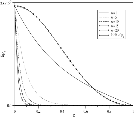
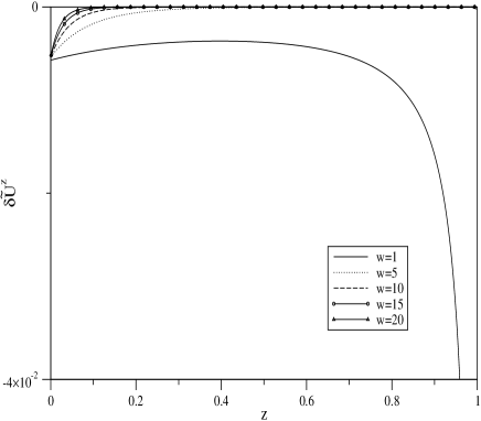
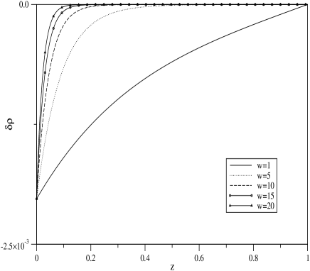
Figure 6: Profiles of the amplitude perturbations modes for the axial pressure, axial physical velocity and energy density for the case when $R=0.1$ and $w=1,5,10,15,20$. To ensure that the perturbations are in accordance with the stability criterion imposed, we have depicted in the pressure perturbation graph the 10% profile of the axial pressure. In the energy density perturbation graph the 10% profile of the energy density was omitted because the values are two order of magnitudes higher. In the axial velocity perturbation profiles the mode with $w=1$ is not stable. Note that the starting radius of the abrupt increase in the axial velocity perturbation amplitude coincide with the point in which the pressure perturbation becomes greater than the 10% profile.

In Fig. 6 we present the amplitude profiles of the axial pressure perturbation, the axial velocity perturbation and the energy density perturbation for the value of the parameter $R=0.1$. We see that the the pressure perturbation modes are always of the some order of magnitude or lower when compared to the 10% profile. Similar to the Sec. IV-B case, the velocity perturbation amplitude profiles increase abruptly near the edge of the disk at $z=1$. For higher values of the parameter $w$ the modes are stable. Even for the most stable mode there is a abruptly increase in the amplitude profile at the edge of the disk. This change in the behavior occurs very near $z=1$ and can not be seen in the axial velocity perturbation graph. In this case we can say that the mode with $w=1$ is not stable. If we compare the axial velocity perturbation graph of Fig. 6 with Fig. 4, we note that the perturbation modes considered in this subsection have larger regions of stability. The modes that correspond to the energy density perturbations are all stable. Note that we have not plot the 10% profile of the energy density because is at least two order of magnitude higher than the values depicted. We performed the above analysis for different values of the parameter $R$ and we found that the quantities involve have the same qualitative behavior. Similar to Sec. IV-B, some modes corresponding to lower values of the frequency $w$ are not stable. As we note in Fig. 6, this is related to the fact that our first order perturbation is not valid in some regions. In these cases, more complex structures may be form, but in order to study them, we need a higher order perturbation formalism.

IV.5 Perturbation with $\delta U^{R}$, $\delta p_{R}$, $\delta U^{z}$, $\delta p_{z}$ and $\delta p_{R}\equiv\delta p_{z}$

In this subsection we perturb the radial component of the four velocity, the axial component of the four velocity, the radial pressure and the axial pressure. This kind of perturbation belongs to the ones marked with a question mark in Table 1. As we said in Sec. II, we need an extra condition to make the set of equations self-consistent. In this case, we set $\delta p_{R}\equiv\delta p_{z}\equiv\delta p$. Therefore, the set of equations (II)-(II) reduce to a second order partial differential equation for the pressure perturbation $\delta p$, say

$$F_{A}\delta p_{,RR}+F_{B}\delta p_{,R}+F_{C}\delta p_{,zz}+F_{D}\delta p_{,z}+F_{E}\delta p=0,$$ (27)

where ($F_{A},F_{B},F_{C},F_{D},F_{E}$) are functions of ($R,z,w$), see Appendix E. The partial differential equation (27) is solved numerically with four boundary conditions, at $z\approx-1$, $z\approx 1$, $R\approx 0$ and $R=20$. The boundary condition at $z$ can not be set at 1 because some quantities diverge. As we said in Sec. IV-B, this is due to the geometrical restrictions that has the isotropic Schwarzschild thick disk. They are different ways in which we can set the boundary conditions in order to simulate various kinds of pressure perturbations. Here, we treat only the case when we have a pressure perturbation at $R\approx 0$ and along the $z$ axis, i.e. some kind of a rod perturbation. We set the value of the rod pressure perturbation to be 10% of the axial pressure. For the rest of the boundary conditions we set the values equal to zero because we want the perturbation to vanish when approaching the edge of the disk. We chose the 10% of the value of the axial pressure instead of the radial pressure because it has the lowest value near $R\approx 0$. In that way, the perturbation values are also below the 10% values of the radial pressure and the general linear perturbation is valid.

In Fig. 7, we present the perturbation amplitude for the pressure, the physical radial velocity and the physical axial velocity for $w=1$. We see in the pressure perturbation graph that the perturbation rapidly decays to values near zero when we move out from the center of the disk. In the velocity perturbations profiles we can see an interesting phenomenon. Note that in the lower domain of the disk [-1,0) the axial velocity perturbation is positive and in the upper domain (0,1] the axial velocity perturbation is negative. This means that due to the linear perturbation the disk tries to collapse to the plane $z=0$. Now, if we look to the radial velocity perturbation graph, we note that the upper and lower parts depart from the center of the disk due to the positive radial perturbation. The center of the disk tries to condensate. So, with these considerations, we may say that the disk tends to form some kind of a ring around the center of the disk. This phenomenon appears near the center of the disk in a few units of $R$. The parameter $w$ enters only like a scale factor in the differential equations quantities studied.

V Conclusions

In this manuscript we obtain the basic perturbation equations for studying the stability of thick disks. These equations were obtained when we applied a general first order perturbation to the conservation equations of motion. The great number of unknowns make the set of equations not self-consistent. In order to make the system of equations self-consistent we must chose a combination of the perturbed quantities. This opens the possibility for various types of combinations. In this manuscript we made a classification of these possibilities and studied the physical accepted perturbations. We can say, that the stability analysis we performed is more complete than the stability analysis of particle motion along geodesics because we take into account the collective behavior of the particles. However, this analysis can be said to be incomplete because the energy momentum perturbation tensor of the fluid is treated as a test fluid and does not alter the background metric. This is a second degree of approximation to the stability problem in which the emission of gravitational radiation is considered.

The stability analyses made to the isotropic Schwarzschild thick disk, show that this disk is stable when we applied radial and azimuthal perturbations. In the case of axial perturbations, the nodes are not stable near the edge of the disk. The lack of stability is due to the form of the geometric thick disk considered vog:let4 , i.e. it is only valid in a fixed axial interval $-a\leq z\leq a$, where $a$ is a constant (in our case $a$=1). If we discard the region near the axial edge we can say, in general, that for higher values of the parameters $w$ and $k_{\theta}$ the axial modes are also stable. For lower values of $w$, some axial perturbations are not stable. This is related to the fact that our first order perturbation is not valid in some regions of the considered quantities. In these cases, more complex structures may be form, but in order to study them, we need a higher order perturbation formalism.

Appendix A Coefficients of perturbation type A

The general form of the functions ($F_{A},F_{B},F_{C}$) appearing in the second order ordinary differential equation (24) are given by

$$F_{A}=A_{1}\alpha_{1},\hskip 14.22636ptF_{B}=A_{1}{\alpha_{1}}_{,R}+A_{1}\alpha_{2}+A_{3}\alpha_{1},$$

$$F_{C}=A_{1}{\alpha_{2}}_{,R}+A_{3}\alpha_{2}+A_{4}\alpha_{3},$$ (28)

where $\alpha_{1}$, $\alpha_{2}$ and $\alpha_{3}$ are

$$\alpha_{1}=-\frac{B_{1}}{B_{2}},\hskip 14.22636pt\alpha_{2}=\frac{B_{5}D_{4}-B_{4}D_{5}}{B_{2}D_{5}},$$

$$\alpha_{3}=\frac{C_{2}D_{4}}{C_{1}D_{5}}.$$ (29)

In Eqs. (28) and (29), we denote the coefficients of Eq. (II) by $A_{i}$, the coefficient of Eq. (II) by $B_{i}$, the coefficient of Eq. (10) by $C_{i}$, the coefficient of Eq. (II) by $D_{i}$, e.g., the first term in (II) has the coefficient $A_{1}$ multiplied by the factor $\delta U^{R}_{,R}$, the second term has the coefficient $A_{2}$ multiplied by the factor $\delta U^{R}$, etc. The explicit form of the above equations is obtained replacing the fluid variables ($\rho,p_{R},p_{\theta},p_{z}$) of the isotropic Schwarzschild thick disk.

Appendix B Coefficients of perturbation type B

The general form of the functions ($F_{A},F_{B},F_{C}$) appearing in the second order ordinary differential equation (26) are given by

$$F_{A}=A_{2}\alpha_{1},\hskip 14.22636ptF_{B}=A_{2}{\alpha_{1}}_{,z}+A_{2}\alpha_{2}+A_{5}\alpha_{1},$$

$$F_{C}=A_{2}{\alpha_{2}}_{,z}+A_{4}\alpha_{3}+A_{5}\alpha_{2},$$ (30)

where $\alpha_{1}$, $\alpha_{2}$ and $\alpha_{3}$ are

$$\alpha_{1}=-\frac{D_{1}}{D_{2}},\hskip 14.22636pt\alpha_{2}=\frac{B_{6}D_{5}-B_{5}D_{6}}{B_{5}D_{2}},$$

$$\alpha_{3}=\frac{C_{2}B_{6}}{C_{1}B_{5}},$$ (31)

where the meaning of the notation for the coefficients ($A_{i},B_{i},C_{i},D_{i}$) are explained in Appendix A.

Appendix C Coefficients of perturbation type C

The general form of the functions ($F_{A},F_{B},F_{C}$) are given by

$$F_{A}=A_{1}\alpha_{1},\hskip 14.22636ptF_{B}=A_{1}{\alpha_{1}}_{,R}+A_{1}\alpha_{2}+A_{3}\alpha_{1},$$

$$F_{C}=A_{1}{\alpha_{2}}_{,R}+A_{3}\alpha_{2}+A_{6}\alpha_{3},$$ (32)

where $\alpha_{1}$, $\alpha_{2}$ and $\alpha_{3}$ are

$$\alpha_{1}=-\frac{B_{1}}{B_{2}},\hskip 14.22636pt\alpha_{2}=\frac{B_{3}D_{4}-B_{4}D_{3}}{B_{2}D_{3}},$$

$$\alpha_{3}=-\frac{D_{4}}{D_{3}},$$ (33)

where the meaning of the notation for the coefficients ($A_{i},B_{i},D_{i}$) are explained in Appendix A.

Appendix D Coefficients of perturbation type D

The general form of the functions ($F_{A},F_{B},F_{C}$) are given by

$$F_{A}=A_{2}\alpha_{1},\hskip 14.22636ptF_{B}=A_{2}{\alpha_{1}}_{,z}+A_{2}\alpha_{2}+A_{5}\alpha_{1},$$

$$F_{C}=A_{2}{\alpha_{2}}_{,z}+A_{5}\alpha_{2}+A_{6}\alpha_{3},$$ (34)

where $\alpha_{1}$, $\alpha_{2}$ and $\alpha_{3}$ are

$$\alpha_{1}=-\frac{D_{1}}{D_{2}},\hskip 14.22636pt\alpha_{2}=\frac{B_{6}D_{3}-B_{3}D_{6}}{B_{3}D_{2}},$$

$$\alpha_{3}=-\frac{B_{6}}{B_{3}},$$ (35)

where the meaning of the notation for the coefficients ($A_{i},B_{i},D_{i}$) are explained in Appendix A.

Appendix E Coefficients of perturbation type E

The general form of the functions ($F_{A},F_{B},F_{C},F_{D},F_{E}$) appearing in the partial second order differential equation (27) are given by

$$F_{A}=A_{1}\alpha_{1},\hskip 14.22636ptF_{B}=A_{1}{\alpha_{1}}_{,R}+A_{1}\alpha_{2}+A_{3}\alpha_{1},$$

$$F_{C}=A_{2}\alpha_{3},\hskip 14.22636ptF_{D}=A_{2}{\alpha_{3}}_{,z}+A_{2}\alpha_{4}+A_{5}\alpha_{3},$$

$$F_{E}=A_{1}{\alpha_{2}}_{,R}+A_{2}{\alpha_{4}}_{,z}+A_{3}\alpha_{2}+A_{5}\alpha_{4},$$ (36)

where $\alpha_{1}$, $\alpha_{2}$, $\alpha_{3}$ and $\alpha_{4}$ are

$$\alpha_{1}=-\frac{B_{1}}{B_{2}},\hskip 14.22636pt\alpha_{2}=-\frac{B_{4}+B_{6}}{B_{2}},$$

$$\alpha_{3}=-\frac{D_{1}}{D_{2}},\hskip 14.22636pt\alpha_{4}=-\frac{D_{4}+D_{6}}{D_{2}}.$$ (37)

where the meaning of the notation for the coefficients ($A_{i},B_{i},D_{i}$) are explained in Appendix A.

Figure 7: Profiles of the amplitude perturbations modes for the pressure, radial physical velocity and axial physical velocity for the case when $w=1$. We see that the perturbation rapidly goes to values near zero when we depart from the center of the disk, i.e. the perturbations are stable. The parameter $w$ enters as a scale factor in the differential equations and do not alter the qualitative properties of the perturbations.

References

- (1) W.A. Bonnor and A. Sackfield, Commun. Math. Phys. 8, 338 (1968).
- (2) T. Morgan and L. Morgan, Phys. Rev. 183, 1097 (1969).
- (3) L. Morgan and T. Morgan, Phys Rev. D 2, 2756 (1970).
- (4) G.A. González and P.S. Letelier, Class. Quantum Grav. 16, 479 (1999).
- (5) D. Lynden-Bell and S. Pineault, Mon. Not. R. Astron. Soc. 185, 679 (1978).
- (6) J.P.S. Lemos, Class. Quantum Grav. 6, 1219 (1989).
- (7) J.P.S. Lemos and P.S. Letelier, Class. Quantum Grav. 10, L75 (1993).
- (8) J.P.S. Lemos and P.S. Letelier, Phys. Rev. D 49, 5135 (1994).
- (9) J.P.S. Lemos and P.S. Letelier, Int. J. Mod. Phys. D 5, 53 (1996).
- (10) C. Klein, Class. Quantum Grav. 14, 2267 (1997).
- (11) J. Bičák and T. Ledvinka, Phys. Rev. Lett. 71, 1669 (1993).
- (12) G.A. González and O.A. Espitia, Phys. Rev. D 68, 104028 (2003).
- (13) G. García R. and G.A. González, Phys. Rev. D 69, 124002 (2004).
- (14) G.A. González and P.S. Letelier, Phys. Rev. D 62, 064025 (2000).
- (15) M. Chazy, Bull. Soc. Math. France 52, 17 (1924).
- (16) H. Curzon, Proc. London Math. Soc. 23, 477 (1924).
- (17) D.M. Zipoy, J. Math. Phys. 7, 1137 (1966).
- (18) B.H. Voorhees, Phys. Rev. D 2, 2119 (1970).
- (19) J. Bičák, D. Lynden-Bell and J. Katz, Phys. Rev. D 47, 4334 (1993).
- (20) J. Bičák, D. Lynden-Bell and C. Pichon, Mon. Not. R. Astron. Soc. 265, 126 (1993).
- (21) T. Ledvinka, M. Zofka, and J. Bičák, in Proceedings of the 8th Marcel Grossman Meeting in General Relativity, edited by T. Piran (World Scientific, Singapore, 1999), pp. 339-341.
- (22) P.S. Letelier, Phys. Rev. D 60, 104042 (1999).
- (23) J. Katz, J. Bičák and D. Lynden-Bell, Class. Quantum Grav. 16, 4023 (1999).
- (24) D. Vogt and P.S. Letelier, Phys. Rev. D 68, 084010 (2003).
- (25) D. Vogt and P.S. Letelier, Class. Quantum Grav. 21, 3369 (2004)
- (26) D. Vogt and P.S. Letelier, Phys. Rev. D 70, 064003 (2004).
- (27) O. Semerák, in Gravitation: Following the Prague Inspiration, to Celebrate the 60th Birthday of Jiri Bičák, edited by O. Semerák, J. Podolsky, and M. Zofka (World Scientific, Singapure, 2002), p. 111, available at http://xxx.lanl.gov/abs/gr-qc/0204025.
- (28) V. Karas, J-M. Huré and O. Semerák, Class. Quantum Grav. 21, R1 (2004).
- (29) G. Neugebauer and R. Meinel, Phys. Rev. Lett. 75, 3046 (1995).
- (30) C. Klein and O. Richter, Phys. Rev. Lett. 83, 2884 (1999).
- (31) C. Klein, Phys. Rev. D 63, 064033 (2001).
- (32) J. Frauendiener and C. Klein, Phys. Rev. D 63, 084025 (2001).
- (33) C. Klein, Phys. Rev. D 65, 084029 (2002).
- (34) C. Klein, Phys. Rev. D 68, 027501 (2003).
- (35) C. Klein, Ann. Phys. (N.Y.) 12, 599 (2003).
- (36) G.A. González and P.S. Letelier, Phys. Rev. D 69, 044013 (2004).
- (37) D. Vogt and P.S. Letelier, Phys. Rev. D 71, 084030 (2005).
- (38) D. Vogt and P.S. Letelier, Mon. Not. R. Astron. Soc. 363, 268 (2005).
- (39) J. Binney and S. Tremaine, Galactic Dynamics, (Princeton University Press, New Jersey, 1987).
- (40) A.M. Fridman and V.L. Polyachenko, Physics of Gravitating Systems I : Equilibrium and Stability, (Springer-Verlag, New York, 1984).
- (41) P.S. Letelier, Phys. Rev. D 68, 104002 (2003).
- (42) Lord Rayleigh, Proc. R. Soc. London A93, 148 (1916).
- (43) L.D. Landau and E.M. Lifshitz, Fluid Mechanics, 2nd ed. (Pergamon Press, Oxford, 1987), Sec. 27.
- (44) J.M. Bardeen, Astrophys. J. 161, 103 (1970).
- (45) M.A. Abramowicz and A.R. Prasanna, Mon. Not. R. Astron. Soc. 245, 720 (1990).
- (46) O. Semerák and M. Žáček, Publ. Astron. Soc. Japan 52, 1067 (2000).
- (47) O. Semerák and M. Žáček, Class. Quantum Grav. 17, 1613 (2000).
- (48) O. Semerák, Class. Quantum Grav. 20, 1613 (2003).
- (49) F.H. Seguin, Astrophys. J. 197, 745 (1975).
- (50) M. Ujevic and P.S. Letelier, Phys. Rev. D 70, 084015 (2004).
- (51) In the Appendix section of reference uje:let are some typographical errors. In Eq. (A1) we must perform the transformation . In Eq. (B3) there is a factor missing.
- (52) M. Ujevic and P.S. Letelier, A&A 442, 785 (2005).