A solution to the cosmological constant problem

Abstract

We argue that, when coupled to Einstein’s theory of gravity, the Yukawa theory may solve the cosmological constant problem in the following sense: The radiative corrections of fermions generate an effective potential for the scalar field, such that the effective cosmological term $\Lambda_{\rm eff}$ is dynamically driven to zero. Thence, for any initial positive cosmological constant $\Lambda_{0}$, $\Lambda_{\rm eff}=0$ is an attractor of the semiclassical Einstein theory coupled to fermionic and scalar matter fields. When the initial cosmological term is negative, $\Lambda_{\rm eff}=\Lambda_{0}$ does not change. Next we argue that the dark energy of the Universe may be explained by a GUT scale fermion with a mass, $m\simeq 4.3\times 10^{15}~{}{\rm GeV}(\sqrt{\Lambda_{0}}/10^{13}~{}{\rm GeV})^{1/2}$. Finally, we comment on how the inflationary paradigm, BEH mechanism and phase transitions in the early Universe get modified in the light of our findings.

I Introduction

The cosmological constant problem can be stated follows Weinberg:1988cp . Vacuum fluctuations of any particle species contribute to the energy density of the vacuum as,

$$\rho_{0}=\pm\int\frac{d^{3}p}{(2\pi)^{3}}\frac{1}{2}({p^{2}+m^{2}})^{1/2}\,,$$ (1)

where $p$ is the momentum of a particle, $m$ its mass, and the positive (negative) sign stands for bosons (fermions). (In this article we use the natural units in which the speed of light and the reduced Planck constant are set to unity, $c=1$ and $\hbar=1$.) $\rho_{0}$ is a badly divergent quantity. It is often argued that a natural ultraviolet cutoff is the Planck scale, $m_{P}=G_{N}^{-1/2}\simeq 1.22\times 10^{19}~{}{\rm GeV}$, such that,

$$\rho_{0}=\pm\frac{m_{\rm P}^{4}}{16\pi^{2}}\simeq\pm(3.4\times 10^{18}~{}{\rm GeV})^{4}\,,$$ (2)

of equivalently,

$$\Lambda_{0}=\pm\frac{\rho_{0}}{M_{\rm P}^{2}}\simeq\pm 2.4\times 10^{37}~{}{\rm GeV}^{2}\,,$$ (3)

where $M_{\rm P}=(8\pi G_{N})^{-1/2}\simeq 2.4\times 10^{18}~{}{\rm GeV}$ is the reduced Planck mass. Above the Planck scale, an as of yet unknown quantum gravity theory is believed to lead to finite dynamics. The observed value Riess:1998 ; Perlmutter:1998 is at least 120 orders of magnitude smaller,

$$\Lambda_{\rm obs}\leq 3H_{0}^{2}\Omega_{\rm DE}\simeq 5\times 10^{-84}~{}{\rm GeV}^{2}\,,$$ (4)

where we used the current value for the Hubble parameter, $H_{0}\simeq 1.5\times 10^{-42}~{}{\rm GeV}$, and $\Omega_{\rm DE}\simeq 0.74$ is the dark energy contribution.

The discrepancy between (4) and (3) is known as the cosmological constant problem. There is a milder formulation of the problem, according to which supersymmetry takes care of the balance between the positive and negative contributions in (3) above the scale at which supersymmetry is restored. In this case, $\rho_{0}\sim\pm m_{\rm susy}^{4}$, where $m_{\rm susy}$ is the energy scale above which supersymmetry is restored. This works only for global supersymmetry however, since in local supersymmetry (which also includes gravity) this balance does not necessarily hold.

Zeldovich has proposed Zeldovich:1967gd that the discrepancy between the observed (4) and the theoretically more natural value (3) could be explained by a mechanism, where quantum matter fluctuations (2) would cancel an initial geometric cosmological constant of Einstein’s theory. Yet neither he, nor anyone else, has been able to provide a satisfactory compensatory mechanism. In this article we present such a dynamical mechanism, which explains how an initially large and positive $\Lambda_{0}$ can be driven to zero by the gravitational backreaction induced by fermionic quantum fluctuations, such that today the effective cosmological term has a small, but nonvanishing, value.

The cosmological constant has a long history Weinberg:1988cp ; RughZinkernagel:2000 since it was in 1917 introduced by Einstein to his general relativistic theory of gravitation. Around the same time Nernst Nernst:1916 observed that quantum matter (light) fluctuations can contribute to the vacuum energy. In 1968 the vacuum energy was experimentally observed Boyer:1968uf based on the Casimir effect Casimir:1948dh . Here we just briefly mention several attempts to solve the cosmological constant problem. It is well known that (tree level) scalar potentials (e.g. quintessence models PeeblesRatra:2002 ) cannot do the job because of the Weinberg theorem Weinberg:1988cp . This theorem states that one can always add a constant potential energy without dynamical consequences to any scalar field potential which naïvely drives the field towards the value, where its potential energy vanishes. Another possibility is “shadow” matter, which contributes with an opposite sign to the energy density as ordinary matter, and couples only gravitationally. This requires introduction of a lot of new and yet unobserved particle species, and moreover has problems when perturbative gravity corrections are taken into account KaplanSundrum:2005 . The general trend in literature is either to resort to the anthropic principle Weinberg:1988cp , or to postulate new symmetries, an example being the symmetry which relates positive and (as of yet unobserved) negative energy states Linde:1984ir ; KaplanSundrum:2005 ; 'tHooftNobbenhuis:2006 .

When written in the approximation of a homogeneous and isotropic space-time with the metric tensor,

$$g_{\mu\nu}={\rm diag}(-1,a^{2},a^{2},a^{2})\,,$$ (5)

the semiclassical Einstein equations can be written in the following FLRW form,

$$H^{2} \equiv \big{(}\frac{\dot{a}}{a}\Big{)}^{2}=\frac{8\pi G_{N}}{3}\rho+\frac{\Lambda_{0}}{3}-\frac{k}{a^{2}}$$ (6)

$$\frac{\ddot{a}}{a} = -\frac{4\pi G_{N}}{3}(\rho+3{\cal P})+\frac{\Lambda_{0}}{3}\,,$$ (7)

where $a$ denotes the scale factor, $\dot{a}=da/dt$, $\ddot{a}=d^{2}a/dt^{2}$, $H$ is the Hubble parameter, $G_{N}$ the Newton constant, $\Lambda_{0}$ the cosmological term, $\rho$ the energy density, ${\cal P}$ the pressure, and $k$ is the curvature of spatial sections of space-time. Here we take for simplicity $k=0$, which is consistent with current observations Spergel:2006 . In the derivation of Eqs. (6–7) one assumes that the matter stress-energy tensor has an ideal fluid form, and Eqs. (6–7) are written in the fluid rest frame.

We shall now calculate the stress-energy contribution to the Einstein equations (6–7) in the Yukawa theory. In doing so we shall resort to certain approximations, which are needed for analytical calculations.

The dynamics of the matter fields are described by the following model Yukawa theory,

$$S_{\rm Yu}=\int d^{4}x\sqrt{-g}{\cal L}_{\rm Yu}\,,$$ (8)

with the Lagrangian,

$$\sqrt{-g}{\cal L}_{\rm Yu}=\sqrt{-g}\Big{(}\bar{\psi}i\nabla\!\!\!\!/\psi-m_{0}\bar{\psi}\psi-\frac{1}{2}g^{\mu\nu}(\partial_{\mu}\varphi)(\partial_{\nu}\varphi)-V_{0}(\varphi)-\frac{1}{2}\xi_{0}{\cal R}\varphi^{2}-f_{0}\varphi\bar{\psi}\psi\Big{)}\,,$$ (9)

where $\nabla\!\!\!\!/=e^{\mu}_{b}\gamma^{b}(\partial_{\mu}-\Gamma_{\mu})$ denotes the covariant derivative acting on spinors, $e^{\mu}_{b}$ is the tetrad field, $\Gamma_{\mu}$ is the spin(or) connection, $m_{0}$ is the bare fermion mass, $\psi$ and $\varphi$ denote the fermionic and scalar fields, respectively, $V_{0}=(1/2)\mu_{0}^{2}\varphi^{2}+\lambda_{0}\varphi^{4}/4!$ is the (tree level) scalar potential, $\mu_{0}$ and $\lambda_{0}$ are the bare scalar mass and quartic self-coupling, respectively, ${\cal R}$ is the Ricci curvature scalar, $g={\rm det}(g_{\mu\nu})$, and $f_{0}$ is the Yukawa coupling.

Note that fermions appear quadratically in the action, so in principle they can be integrated out. In practice though, this can be done only in a handful of gravitational backgrounds. Since we are interested in solving the problem in a background given by a (positive or negative) cosmological term plus matter contribution, we make the first of our crude approximations and assume that the gravitational background is well approximated by (anti-)de Sitter space-time. Below we comment on how good this approximation is. The problem of integrating fermions in de Sitter background has recently been solved by Miao and Woodard MiaoWoodard:2006 , whereby they neglected scalar field fluctuations. This approximation is accurate to leading log, where the log refers to $\ln(a)$, and $a$ is the scale factor of the Universe (see Eq. (14) below). The leading log approximation is accurate in de Sitter background Woodard:2005cw . Certain aspects of the work in Ref. MiaoWoodard:2006 are inspired by an earlier work of Candelas and Raine CandelasRaine:1975 . Various quantum aspects of the Yukawa theory in de Sitter background have formerly been studied in Refs. GarbrechtProkopec:2006 ; MiaoWoodard:2005 ; ProkopecWoodard:2003 , and a new fermion mass generation mechanism has been found GarbrechtProkopec:2006 .

II de Sitter and anti-de Sitter spaces

de Sitter space is perhaps best viewed as a 4-dimensional hyperboloid embedded into the five-dimensional Minkowski space-time with the line element,

$$ds_{5}^{5}=-dX_{0}^{2}+dX_{1}^{2}+dX_{2}^{2}+dX_{3}^{2}+dX_{4}^{2}\,.$$ (10)

The embedded hyperboloid of de Sitter space is shown in figure 1, and it is determined by

$$-X_{0}^{2}+X_{1}^{2}+X_{2}^{2}+X_{3}^{2}+X_{4}^{2}=\frac{1}{H^{2}}\,,$$ (11)

where $H$ denotes the Hubble parameter. The symmetry of de Sitter space, $SO(1,4)$, is manifest in this embedding. One can define de Sitter invariant distance functions,

$$Z(X;X^{\prime})=H^{2}\sum_{A,B=0}^{4}\eta_{AB}X_{A}X^{\prime}_{B}=1-\frac{1}{2}Y(X;X^{\prime})\,,\qquad\eta_{AB}={\rm diag}(-1,1,1,1,1)\,.$$ (12)

We shall use the following flat four-dimensional coordinates (which cover 1/2 of de Sitter manifold),

$$X_{0} = \frac{1}{H}\sinh(Ht)+\frac{H}{2}{\rm e}^{Ht}\|\vec{x}\|^{2}\,,\qquad(-\infty<t<\infty)$$

$$X_{i} = {\rm e}^{Ht}x_{i}\,\qquad(-\infty<x_{i}<\infty)\,,\qquad(i=1,2,3)$$

$$X_{4} = \frac{1}{H}\cosh(Ht)-\frac{H}{2}{\rm e}^{Ht}\|\vec{x}\|^{2}\,,$$ (13)

in which the metric tensor reduces to the form (5), with the scale factor, $a={\rm e}^{Ht}$. When written in terms of conformal time $\eta$, defined as $ad\eta=dt$, the metric tensor acquires the conformal form,

$$g_{\mu\nu}=a^{2}\eta_{\mu\nu}\,,\qquad a=-\frac{1}{H\eta}\quad(\eta<0)\,,\qquad\eta_{\mu\nu}={\rm diag}(-1,1,1,1)\,.$$ (14)

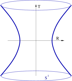
Figure 1: The embedding of de Sitter space into a five dimensional flat space-time. The vertical line corresponds to the time coordinate, $X_{0}=T$, and the radial coordinate, $R=({X_{1}^{2}+X_{2}^{2}+X_{3}^{2}+X_{4}^{2}})^{1/2}=1/H$. At each point $(T,R)$ there is a unit 3-sphere, $S^{3}$ (which has in this figure collapsed to $S^{1}$).

The invariant distance functions, $Z(X;X^{\prime})\equiv z(x;x^{\prime})$ and $Y(X;X^{\prime})\equiv y(x;x^{\prime})$, reduce in these coordinates to the simple form,

$$z(x;x^{\prime})=1-\frac{1}{2}y(x;x^{\prime})\,,\qquad y(x;x^{\prime})=aa^{\prime}H^{2}\Delta x^{2}$$ (15)

with $a=a(\eta)=-1/(H\eta)$, $a^{\prime}=a(\eta^{\prime})=-1/(H\eta^{\prime})$, and

$$\Delta x^{2}(x;x^{\prime})=-(|\eta-\eta^{\prime}|-i\epsilon)^{2}+\|\vec{x}-\vec{x}^{\prime}\|^{2}\,,$$ (16)

where (for later use) we introduced an infinitesimal $\epsilon>0$. In these coordinates the curvature of spatial sections vanishes, and thus they are also known as flat (Euclidean) coordinates, in which de Sitter space appears as uniformly expanding.

For the integration of fermions we also need the fermion propagator,

$$iS(x;x^{\prime})=\langle x|\frac{i}{\sqrt{-g}(i\nabla\!\!\!\!/-m)}|x^{\prime}\rangle\,,\qquad(m\equiv m_{0}+f_{0}\varphi)\,.$$ (17)

This propagator can be solved in de Sitter background and in the approximation of a nearly constant $\varphi$ ($\partial_{\mu}\varphi$ and higher order derivatives are neglected), and the solution can be written in the form CandelasRaine:1975 MiaoWoodard:2006 ,

$$iS(x;x^{\prime})=a\Big{(}i\nabla\!\!\!\!/+m\Big{)}(aa^{\prime})^{-\frac{1}{2}}\sum_{\pm}iS_{\pm}(y)\frac{1\pm\gamma^{0}}{2}$$ (18)

where $i\nabla\!\!\!\!/=a^{-\frac{D+1}{2}}i\gamma^{\mu}\partial_{\mu}a^{\frac{D-1}{2}}$, and $iS_{\pm}=iS_{\pm}(y)$ are the following de Sitter invariant scalar functions (which contain no spinor structure),

$$iS_{\pm}=\frac{H^{D-2}}{(4\pi)^{\frac{D}{2}}}\frac{\Gamma\Big{(}\frac{D}{2}-1\mp i\frac{m}{H}\Big{)}\Gamma\Big{(}\frac{D}{2}\pm i\frac{m}{H}\Big{)}}{\Gamma\Big{(}\frac{D}{2}\Big{)}}\;{{}_{2}F_{1}}\Big{(}\frac{D}{2}-1\mp i\frac{m}{H},\frac{D}{2}\pm i\frac{m}{H};\frac{D}{2};1-\frac{y}{4}\Big{)}\,,$$ (19)

where $m=m(\varphi)$ is defined in Eq. (17), $D$ denotes the number of space-time dimensions, ${{}_{2}F_{1}}$ is the hypergeometric function, and $\gamma^{\mu}$ are the Dirac $\gamma$-matrices. With the $\epsilon$ pole prescription as in (15–16), one can show that the propagator (18–19) indeed solves the Dirac equation in de Sitter space,

$$\sqrt{-g}(i\nabla\!\!\!\!/-m)iS(x;x^{\prime})=i\delta^{D}(x-x^{\prime})\,,$$ (20)

where $\delta^{D}(x-x^{\prime})$ denotes the $D$-dimensional Dirac $\delta$-distribution and $\varphi=$ const.

Similarly to de Sitter space, anti-de Sitter space can be thought of as the hyperboloid,

$$-X_{0}^{2}-X_{1}^{2}+X_{2}^{2}+X_{3}^{2}+X_{4}^{2}=-R^{2}\equiv-\frac{1}{H^{2}}\,,$$ (21)

embedded into the five-dimensional flat space-time with the line element,

$$ds_{5}^{5}=-dX_{0}^{2}-dX_{1}^{2}+dX_{2}^{2}+dX_{3}^{2}+dX_{4}^{2}\,,$$ (22)

which possesses an SO(2,3) symmetry. The graphical representation of anti-de Sitter space is the same as in figure 1, except that each point on the vertical axis corresponds to a circle, and the points of constant radii, $R=(X_{2}^{2}+X_{3}^{2}+X_{4}^{2})^{1/2}$, correspond to two-dimensional spheres $S^{2}$. The definition of anti-de Sitter invariant distance functions is as in de Sitter space (12), with the five dimensional metric given by, $\eta_{AB}={\rm diag}(-1,-1,1,1,1)$.

The following coordinates, which cover a 1/2 of anti-de Sitter space, are analogous to the flat de Sitter coordinates (13),

$$X_{0} = \frac{1}{2u}+\frac{u}{2}\Big{(}R^{2}+x_{2}^{2}+x_{3}^{2}-\eta^{2}\Big{)}\,\qquad(-\infty<\eta<\infty,u>0)$$

$$X_{1} = Ru\eta$$

$$X_{i} = Rux_{i}\qquad(i=2,3)\,\qquad(-\infty<x_{i}<\infty)$$

$$X_{4} = \frac{1}{2u}-\frac{u}{2}\Big{(}R^{2}-x_{2}^{2}-x_{3}^{2}+\eta^{2}\Big{)}\,,$$ (23)

With the additional replacement, $u=1/x_{1}$, these coordinates yield the conformal metric tensor,

$$g_{\mu\nu}=a^{2}\eta_{\mu\nu}\,,\qquad a=\frac{1}{Hx_{1}}\quad(x_{1}>0)\,,\qquad H=\frac{1}{R}\,.$$ (24)

One should not confuse $H$ in anti-de Sitter space (where it denotes the inverse radius of curvature of the space) with the Hubble parameter $H$ in de Sitter space. Note that unlike de Sitter space, which represents an expanding space time in conformal flat coordinates, the conformal flat coordinates of anti-de Sitter space (24) correspond to a static slicing with the space-time curved in one spatial direction, which we choose to be $x_{1}$. One can easily calculate the anti-de Sitter invariant distance function, $\bar{Z}=-H^{2}\sum_{A,B}\eta_{AB}X_{A}X_{B}^{\prime}=1+\bar{Y}/2$. Upon defining, $y(x;x^{\prime})\equiv\bar{Y}(X;X^{\prime})$ and $z(x;x^{\prime})\equiv\bar{Z}(X;X^{\prime})$, we find in these coordinates,

$$z(x;x^{\prime})=1+\frac{1}{2}y(x;x^{\prime})\,,\qquad y=aa^{\prime}H^{2}\Delta x^{2}\,,$$ (25)

where here $a=a(x_{1})=1/(Hx_{1})$, $a^{\prime}=a({x_{1}}^{\prime})=1/(H{x_{1}}^{\prime})$ $(x_{1},{x_{1}}^{\prime}>0)$ and $\Delta x^{2}$ is given in Eq. (16).

One can show that the anti-de Sitter fermion propagator in the presence of an approximately constant scalar field reduces to the form ProkopecRigopoulos:2006 ,

$$i\bar{S}(x;x^{\prime})=a\Big{(}i\nabla\!\!\!\!/+m\Big{)}(aa^{\prime})^{-\frac{1}{2}}\sum_{\pm}i\bar{S}_{\pm}(y)\frac{1\pm i\gamma^{1}}{2}\,,$$ (26)

where $i\bar{S}_{\pm}=i\bar{S}_{\pm}(y)$ are the anti-de Sitter invariant scalar functions,

$$i\bar{S}_{\pm}={\rm e}^{i(D-2)\pi/2}\frac{H^{D-2}}{(4\pi)^{\frac{D}{2}}}\frac{\Gamma\Big{(}\frac{D}{2}-1\mp\frac{m}{H}\Big{)}\Gamma\Big{(}\frac{D}{2}\pm\frac{m}{H}\Big{)}}{\Gamma\Big{(}\frac{D}{2}\Big{)}}\;{{}_{2}F_{1}}\Big{(}\frac{D}{2}-1\mp\frac{m}{H},\frac{D}{2}\pm\frac{m}{H};\frac{D}{2};1+\frac{y}{4}\Big{)}\,,$$ (27)

and $m\equiv m_{0}+f_{0}\varphi$. Note that the two propagators (18–19) and (26–27) are related by the analytic continuation,

$$H\rightarrow iH\,.$$ (28)

The extra phase in (27) comes from the term in the propagator proportional to $y^{1-D/2}$. This term gives rise to the $\delta$-function in the propagator equation (20), which induces an extra phase due to, $y=aa^{\prime}H^{2}\Delta x^{2}\rightarrow-y$. The spinor structure of the two propagators is related such that the positive and negative energy projectors are replaced as, $(1\pm\gamma^{0})/2\rightarrow(1\pm i\gamma^{1})/2$. The extra imaginary $i$ in the projectors, $(1\pm i\gamma^{1})/2$, is important, since it assures that the spinor structure drops out from the differential operator acting on the propagator.

III Effective potentials

When one uses the anti-de Sitter propagator (26–27) to calculate the effective action by an analogous procedure as done in Refs. CandelasRaine:1975 and MiaoWoodard:2006 , one obtains the following (renormalised) effective potential,

$$\bar{V}(\varphi)=V_{\rm tree}(\varphi)+\frac{H^{4}}{8\pi^{2}}\bigg{[}2\gamma_{E}\Big{(}\frac{m}{H}\Big{)}^{2}+(\zeta(3)\!-\!\gamma_{E})\Big{(}\frac{m}{H}\Big{)}^{4}\!+\!2\int_{x_{0}}^{m/H}\!\!\!dx(x-x^{3})\Big{(}\psi(1+x)+\psi(1-x)\Big{)}\bigg{]}\,,\quad$$ (29)

where,

$$V_{\rm tree}(\varphi)=\frac{1}{2}\mu^{2}\varphi^{2}+\frac{\lambda}{4!}\varphi^{4}-\frac{1}{2}{\cal R}\xi\varphi^{2}\,,$$ (30)

$\psi(z)=(d/dz)\ln(\Gamma(z))$ is the digamma function, and $\lambda$, $\mu$ and $\xi$ are the renormalised parameters (in Ref. MiaoWoodard:2006 the renormalisation has been chosen such that these parameters vanish), $\zeta(3)\simeq 1.202$ is the Riemann zeta function, and $\gamma_{E}\simeq 0.577$ is the Euler constant. This effective potential is induced by fermionic fluctuations in the presence of a nearly constant scalar field in anti-de Sitter space. Since the integrand has simple poles at $x=2,3,4,..$, the lower limit of integration can be taken as $x_{0}=0$ for $m/H<2$, and $x_{0}=[m/H]+c_{AdS}$ when $m/H>2$, where $0<c_{AdS}<1$ is a constant, and $[\cdot]$ denotes the integer part. For $m/H>2$ the potential (29) contains an unspecified constant, which has no dynamical relevance (the dynamical relevance is associated with $-dV/d\varphi$).

Just like the propagators, the effective potentials are related by the analytic continuation (28), such that the de Sitter effective potential reads MiaoWoodard:2006 ,

$$V(\varphi)=V_{\rm tree}(\varphi)+\frac{H^{4}}{8\pi^{2}}\bigg{[}\!-\!2\gamma_{E}\Big{(}\frac{m}{H}\Big{)}^{2}\!+\!(\zeta(3)\!-\!\gamma_{E})\Big{(}\frac{m}{H}\Big{)}^{4}\!-\!2\int_{0}^{m/H}\!\!\!dx(x+x^{3})\Big{(}\psi(1\!+\!ix)+\psi(1\!-\!ix)\Big{)}\bigg{]}\,.\quad$$ (31)

The large field limit of this effective potential is,

$$V\simeq-\frac{m^{4}}{8\pi^{2}}\ln\Big{(}\frac{m}{H}\Big{)}\qquad(m\gg H)\,.$$ (32)

The potentials (29–31) determine the dynamics of scalar fields in de Sitter and anti-de Sitter backgrounds. The dynamics in de Sitter space is given either by the corresponding Euler-Lagrange equations,

$$\partial_{t}^{2}\varphi-\frac{1}{a^{2}}{\vec{\partial}}^{\,2}\varphi+3H\partial_{t}\varphi=-\frac{dV}{d\varphi}\,,$$ (33)

or by the Starobinsky stochastic theory StarobinskyYokoyama:1994 Woodard:2005cw , according to which

$$\partial_{t}\varphi=-\frac{1}{3H}\frac{dV}{d\varphi}+\xi\\ \,,$$ (34)

where $\xi$ is the white noise

$$\langle\xi(x)\xi(x^{\prime})\rangle=\frac{H^{3}}{4\pi^{2}}\delta(t-t^{\prime})\frac{\sin(Ha\|\vec{x}-\vec{x}^{\prime}\|)}{Ha\|\vec{x}-\vec{x}^{\prime}\|}\,,$$ (35)

generated in accelerating space-times as vacuum fluctuations get stretched beyond the Hubble radius, $1/H$. When the effects of quantum tunneling and stochastic fluctuations are neglected, the field generally evolves in the direction of decreasing potential, $dV/d\varphi<0$.

In anti-de Sitter space the dynamics is determined by the Euler-Lagrange equation,

$$\frac{1}{a^{2}}\partial_{\eta}^{2}\varphi-\frac{1}{a^{2}}{\vec{\partial}}^{\,2}\varphi+2H\frac{1}{a}\frac{\partial}{\partial x_{1}}\varphi=-\frac{d\bar{V}}{d\varphi}$$ (36)

where $\bar{V}$ is given in (29). Note that the “damping” (third) term in anti-de Sitter space generates inhomogeneities and thus has a different meaning from its de Sitter counterpart in Eq. (33). Just like in de Sitter space, the Euler-Lagrange equation (36) tells as that the field $\varphi$ is driven in the direction of decreasing potential (along which $-d\bar{V}/d\varphi$ is positive).

In the large field limit ($m=m_{0}+f_{0}\varphi\gg H$), the effective potential (31) reduces to the form that deceptively looks like the Coleman-Weinberg effective potential ColemanWeinberg:1973 ; CandelasRaine:1975 ; MiaoWoodard:2006 , which exhibits the well known instability, according to which fermion fluctuations drive the scalar field to infinity, $\varphi\rightarrow\infty$, whereby $V\rightarrow-\infty$. This instability has been declared a problem. As we shall argue, when interpreted correctly, this runaway feature is the cure.

IV Stress-energy tensor

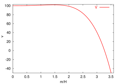
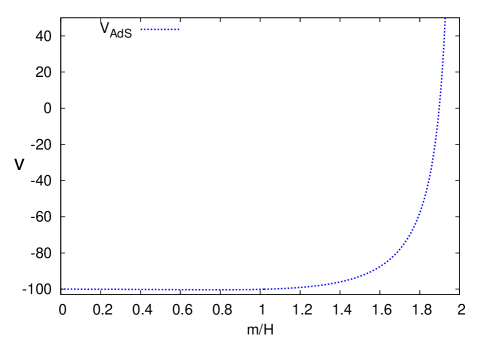
Figure 2: Naïve potential energies, $v=v_{0}+(16\pi^{2}/H^{4})V_{s}$, as a function of $m/H=(m_{0}+f_{0}\varphi)/H$ for de Sitter (left plot) and anti-de Sitter background space (right plot). Note that, as $\varphi$ increases, the potential energy decreases (increases) in de Sitter (anti-de Sitter) space. For definiteness, we chose $\xi=0$, $\mu=0$, $\lambda=0$ and $v(0)=100\,(-100)$ in de Sitter (anti-de Sitter) space.

We have so far said nothing about the back-reaction of matter fields onto gravity, as indicated in Eqs. (6–7). To address this question, we need to calculate the stress-energy tensor of the Yukawa theory (9), which is obtained by the variation of the action (8) with respect to the metric tensor (or tetrad). The relevant part of the stress-energy tensor is (here we suppress terms, which involve space-time derivatives acting on scalar fields, and whose contribution tend to be suppressed in accelerating space-times),

$$T_{\mu\nu} = \frac{a}{2}{\rm lim}_{x\rightarrow x^{\prime}}\Big{(}i\gamma_{(\mu}\nabla_{\nu)}iS(x;x^{\prime})-iS(x;x^{\prime})\overleftarrow{\nabla}^{\prime}_{(\mu}i\gamma_{\nu)}\Big{)}-\xi_{0}G_{\mu\nu}\varphi^{2}+\frac{1}{2}\mu_{0}^{2}\phi^{2}+\frac{\lambda_{0}}{4!}\phi^{4}+{\cal O}\Big{(}(\partial\varphi)^{2}\Big{)}\,,\qquad$$ (37)

where $\gamma_{(\mu}\nabla_{\nu)}$ denotes symmetrisation with respect to $\mu$ and $\nu$, and $G_{\mu\nu}={\cal R}_{\mu\nu}-\frac{1}{2}g_{\mu\nu}{\cal R}$ denotes the Einstein curvature tensor. Upon evaluating $T_{\mu\nu}$ in anti-de Sitter background and performing dimensional regularisation and renormalisation, one obtains ProkopecRigopoulos:2006 ($m=m_{0}+f_{0}\varphi$),

$$\bar{T}_{\mu\nu} = -\bar{V}_{s}(\varphi)g_{\mu\nu}+{\cal O}\Big{(}(\partial\varphi)^{2}\Big{)}$$

$$\bar{V}_{s}(\varphi) = V_{\rm tree}$$

$$\hskip-42.67912pt+\frac{H^{4}}{16\pi^{2}}\Bigg{[}(2\gamma_{E}\!-\!1)\Big{(}\frac{m}{H}\Big{)}^{2}\!+\!\Big{(}\frac{1}{2}\!+\!2\zeta(3)\!-\!2\gamma_{E}\Big{)}\Big{(}\frac{m}{H}\Big{)}^{4}+\Big{(}\frac{m}{H}\Big{)}^{2}\bigg{(}1\!-\!\Big{(}\frac{m}{H}\Big{)}^{2}\bigg{)}\bigg{(}\psi\Big{(}1\!+\!\frac{m}{H}\Big{)}+\psi\Big{(}1\!-\!\frac{m}{H}\Big{)}\bigg{)}\Bigg{]}\,.$$

The de Sitter potential energy is, as expected, obtained by the analytic continuation (28) of Eq. (IV),

$$V_{s}(\varphi) = V_{\rm tree}$$

$$\hskip-42.67912pt-\frac{H^{4}}{16\pi^{2}}\Bigg{[}(2\gamma_{E}\!-\!1)\Big{(}\frac{m}{H}\Big{)}^{2}\!-\!\Big{(}\frac{1}{2}\!+\!2\zeta(3)\!-\!2\gamma_{E}\Big{)}\Big{(}\frac{m}{H}\Big{)}^{4}+\Big{(}\frac{m}{H}\Big{)}^{2}\bigg{(}1\!+\!\Big{(}\frac{m}{H}\Big{)}^{2}\bigg{)}\bigg{(}\psi\Big{(}1\!+\!i\frac{m}{H}\Big{)}+\psi\Big{(}1\!-\!i\frac{m}{H}\Big{)}\bigg{)}\Bigg{]}\,,$$

which agrees with the result obtained in MiaoWoodard:2006 . We plot these two potential energies in figure 2. Note that the de Sitter potential energy shows instability and decays for large values of the argument, while the anti-de Sitter potential is stable. As the argument approaches, $m/H\rightarrow 2$, anti-de Sitter potential grows and diverges as, $\bar{V}_{s}\rightarrow+\infty$, such that the two curves cross. For each point on the de Sitter curve, there is an anti-de Sitter curve which crosses it. If they were both correct, the field dynamics would drive the field both towards larger values (along the de Sitter curve) as well as towards smaller values (along the anti-de Sitter curve). Obviously, both cannot simultaneously correspond to the correct dynamics.

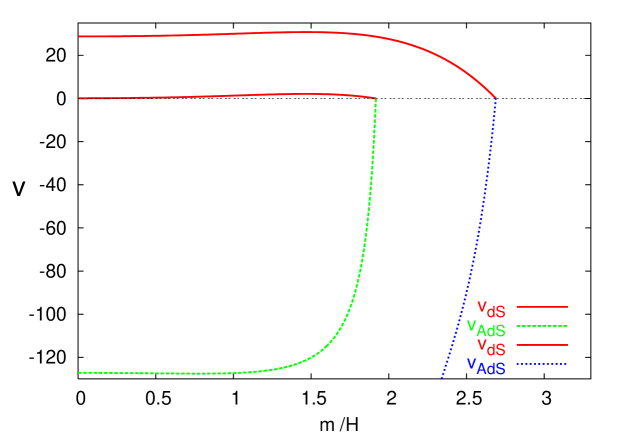
Figure 3: Improved, but still naïve, potential energies, $v_{s}=v_{0}+(16\pi^{2}/H^{4})V_{s}$, as a function of $m/H=(m_{0}+f_{0}\varphi)/H$ for de Sitter and anti-de Sitter space-times. Two (anti-)de Sitter curves are shown. The initial potential energy for the de Sitter and anti-de Sitter case is chosen such that they match at $V_{\rm eff}=0$. As in figure 2, we chose, $\xi=0$, $\mu=0$, $\lambda=0$.

This inconsistency is resolved by noting that de Sitter potentials are valid for all $\rho_{\rm eff}\geq 0$, while anti-de Sitter potentials are valid for $\rho_{\rm eff}\leq 0$, $\rho_{\rm eff}=0$ ($H=0$) being the limiting case, where

$$\rho_{\rm eff}\approx V_{\rm eff}\equiv\cases{V_{s}+M_{\rm P}^{2}\Lambda_{0}\,,&for $V_{\rm eff}\geq 0$ and $\Lambda_{0}\geq 0$\cr\bar{V}_{s}+M_{\rm P}^{2}\Lambda_{0}\,,&for $V_{\rm eff}\leq 0$ and $\Lambda_{0}\leq 0$\cr}\,.$$ (40)

Here $M_{\rm P}^{2}=(8\pi G_{N})^{-1}\simeq 2.4\times 10^{18}~{}{\rm GeV}$ denotes the reduced Planck mass. This leads to an improved dynamics, two examples of which are shown in figure 3. Note that the anti-de Sitter potential energy has simple poles at $m=nH$, where $n=2,3,4,..$ are the integers greater than or equal to 2, such that, for example, the second anti-de Sitter curve in figure 3 runs off to minus infinity at $m=2H$. The first reaction of a learned reader may be: if this picture were true, that would be disastrous, since that would imply that Minkowski space with $\Lambda_{\rm eff}=0$ would be unstable, and decay into anti-de Sitter space, from where it would run either to some large and negative value of $\Lambda_{\rm eff}$ (when $m/H<2$ at $V_{\rm eff}=0$) or even worse to $\Lambda_{\rm eff}\rightarrow-\infty$ (when $m/H>2$ at $V_{\rm eff}=0$). This results in a very uncomfortable observation that an unfortunate field fluctuation or a tunneling event might take us to anti-de Sitter space, resulting in dire consequences. There is one way we can be saved: if the field evolution slows down dramatically as one approaches $\Lambda_{\rm eff}=0$ from above, we would never reach anti-de Sitter. As we shall argue, this is indeed what happens. Even better, we shall see that the naïve interpretation in figure 3 is incorrect. In fact, the de Sitter and anti-de Sitter curves do not continuously connect at $\Lambda_{\rm eff}=0$, as suggested by figure 3, and the curves with $m>2H$ are in fact unphysical. Moreover, $\Lambda_{\rm eff}=0$ is the stable end-point of the evolution for all $\Lambda_{0}\geq 0$. We shall also see that the probability to tunnel to anti-de Sitter space is vanishingly small.

V Dynamical relaxation of the cosmological term

The true dynamics in de Sitter space are obtained by taking account of the matter back-reaction via the Einstein equation (6). When kinetic energies are neglected with respect to the potential energy $V_{\rm eff}$ in (40), which is justified in de Sitter and quasi-de Sitter space-times (slow-roll regime of primordial inflation), the Friedmann equation (6) reduces to,

$$H^{2}\simeq\frac{V_{\rm eff}}{3M_{\rm P}^{2}}\equiv\frac{1}{3}\Big{(}\Lambda_{0}+\frac{V_{s}}{M_{\rm P}^{2}}\Big{)}\equiv\frac{\Lambda_{\rm eff}}{3}\,,$$ (41)

with the scalar field dynamics given by Eq. (33) or by Eqs. (34–35).

Taking account of the matter backreaction means simply that Eq. (41) should be understood as $H=H(\varphi)$. The true potential energy $V_{\rm eff}=V_{\rm eff}(\varphi)$ (or equivalently the effective cosmological term, $\Lambda_{\rm eff}=V_{\rm eff}/M_{\rm P}^{2}$) is then given by the self-consistent solution of equations (41) and (IV).

To get analytical insight into the field dynamics, observe that in the limit when $m/H=(m_{0}+f_{0}\varphi)/H\gg 1$, the potential energy (IV) reduces to the form,

$$V_{s}(\varphi)\simeq V_{\rm tree}-\frac{H^{4}}{8\pi^{2}}\Bigg{[}\Big{(}\frac{m}{H}\Big{)}^{4}\Big{[}\ln\Big{(}\frac{m}{H}\Big{)}-\frac{1}{4}+\gamma_{E}-\zeta(3)\Big{]}+\Big{(}\frac{m}{H}\Big{)}^{2}\Big{[}\ln\Big{(}\frac{m}{H}\Big{)}-\frac{5}{12}+\gamma_{E}\Big{]}+\frac{11}{120}\Bigg{]}\,,$$ (42)

where $V_{\rm tree}$ is given in Eq. (30). At a first sight the potential (42) seems to be of the Coleman-Weinberg type ColemanWeinberg:1973 , whereby $H$ is interpreted as a renormalisation scale. Moreover, for a sufficiently large expectation value of the field, the potential seems to be unstable and naïvely drives the field into anti-de Sitter space. Yet when Eq. (41) is taken account of, the picture completely changes. To see this we insert (42) into (41) to get,

$$H^{2}=\frac{\Lambda_{0}}{3}-\frac{m^{4}}{3\pi m_{\rm P}^{2}}\ln\Big{(}\frac{m}{H}\Big{)}\,,\qquad\qquad(m\gg H)\,,$$ (43)

where $m_{\rm P}=G_{N}^{-1/2}\simeq 1.22\times 10^{19}~{}{\rm GeV}$ and we kept only the leading order term in (42). If we want to solve this for $H$ or $\Lambda_{\rm eff}$ as a function of $m$, the following form of (43) is suitable for iterative procedure,

$$H=m\exp\Big{(}-\frac{\pi m_{\rm P}^{2}\Lambda_{0}}{m^{4}}+\frac{3\pi m_{\rm P}^{2}}{m^{2}}\frac{H^{2}}{m^{2}}\Big{)}\,.$$ (44)

When $H^{2}\ll m^{4}/(3\pi m_{\rm P}^{2})\simeq(\Lambda_{0}/3)/\ln(m/H)$ (which is a stronger condition than $m\gg H$), already the leading order iteration becomes a good approximation,

$$H=m\exp\Big{(}-\frac{\pi m_{\rm P}^{2}\Lambda_{0}}{m^{4}}\Big{)}\qquad\Big{(}H^{2}\ll\frac{m^{4}}{3\pi m_{\rm P}^{2}}\Big{)}\,.$$ (45)

A careful look at (45) reveals something quite bizarre. The potential energy corresponding to (45) is simply,

$$V_{s} = -\Lambda_{0}M_{\rm P}^{2}+V_{\rm res}$$

$$V_{\rm res} = 3m^{2}M_{\rm P}^{2}\exp\Big{(}-\frac{2\pi m_{\rm P}^{2}\Lambda_{0}}{m^{4}}\Big{)}\,,$$ (46)

which is of a completely different form than the perturbative-looking potential (42). Moreover, the potential (46) is nonperturbative with respect to both gravitational and Yukawa coupling constants. Furthermore, one can show that the full solution of Eq. (43) is also nonperturbative with respect to $\Lambda_{0}$. Recall that, after integrating the fermions in a nontrivial background (de Sitter) space-time, we obtained a seemingly perturbative effective potential. Yet, when the matter backreaction onto gravity is taken account of, the resulting effective potential becomes nonperturbative both in the Yukawa coupling, as well as in the gravitational coupling constants (the latter is quite common in classical gravity).

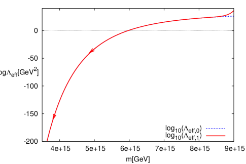
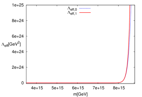
Figure 4: The effective cosmological term $\Lambda_{\rm eff}=3H^{2}$ as a function of $m=m_{0}+f_{0}\varphi$. The left pannel shows $\log_{10}(\Lambda_{\rm eff})$, the right pannel $\Lambda_{\rm eff}$. As $m$ decreases, $\Lambda_{\rm eff}$ approaches zero faster than exponentially. The dashed (blue) and solid (red) curves correspond to the $0$th and $1$st order iterative solutions of Eq. (44), respectively. From the left pannel we see that the effective cosmological term, $\Lambda_{\rm eff}=5\times 10^{-84}~{}{\rm GeV}^{2}$ in Eq. (4), corresponding to the dark energy density of the Universe today, implies for the fermion mass, $m=4.3\times 10^{15}~{}{\rm GeV}$ (where we chose $\sqrt{\Lambda_{0}}=10^{13}~{}{\rm GeV}$).

The effective cosmological term as inferred from Eq. (45) is,

$$\Lambda_{\rm eff}=3m^{2}\exp\Big{(}-\frac{2\pi m_{\rm P}^{2}\Lambda_{0}}{m^{4}}\Big{)}\,,$$ (47)

which approaches zero if $m$ approaches zero. Recall that $m=m_{0}+f_{0}\varphi$, such that this holds independently of the initial fermion mass $m_{0}$. What remains to be shown is that $m\rightarrow 0$ at late times. It suffices to show that the potential energy (46) (at this level of approximation, $V=V_{s}$, cf. Eq. (32)) drives the system towards $m=0$ at late times, where $\Lambda_{\rm eff}=0$. Indeed, since within our approximations, $-V^{\prime}=-V_{s}^{\prime}\propto-m^{\prime}=-f_{0}<0$ ($V^{\prime}\equiv dV/d\varphi$), the force pulls the field towards the origin at $m=0$, where both the potential energy $V_{s}$ and $H^{2}=\Lambda_{\rm eff}/3$ exhibit essential singularity. Visually this can be seen in figure 4, in which we plot the effective cosmological term (47) as a function of $m$. The arrows in figure 4 indicate the direction along which the field evolves. To conclude, we found that the cosmological constant problem is solved in the Yukawa theory plus Einstein’s gravity in the following sense: independently of the initial value of the cosmological term $\Lambda_{0}$, as long as it is positive (and smaller than the Planck scale), it is dynamically driven to zero,

$$\Lambda_{\rm eff}\;\stackrel{{\scriptstyle m\rightarrow 0}}{{\longrightarrow}}\;0\,.$$ (48)

Hence $\Lambda_{\rm eff}=0$ is an attractor for any positive initial cosmological constant $\Lambda_{0}>0$ in a Yukawa theory coupled to gravity. This is true for any Yukawa theory whose tree level couplings $\mu$, $\lambda$ and $\xi$ are such that the scalar field does not get stuck forever in a false vacuum.

Next we address the question of tunneling from de Sitter to anti-de Sitter space. The tunneling probability, $P_{\rm tunnel}$, can be estimated in terms of the Euclidean action $S_{E}$ as follows,

$$P_{\rm tunnel} \sim {\rm e}^{-S_{E}}$$

$$S_{E} = \int d^{4}x_{E}\sqrt{g_{E}}M_{\rm P}^{2}\Lambda_{\rm eff}\,.$$ (49)

Working in closed coordinates (which cover whole de Sitter space),

$$ds_{E}^{2}=\frac{1}{H^{2}\sinh^{2}(\eta_{E})}\Big{(}d\eta_{E}^{2}+d\chi^{2}+\sin^{2}(\chi)\big{(}d\theta^{2}+\sin^{2}(\theta)d\phi^{2}\big{)}\Big{)}\,\quad(-\infty\leq\eta_{E}\leq\infty,\;0\leq\chi\leq\pi)\,,$$ (50)

we have $\sqrt{g_{E}}=H^{-4}\sin^{2}(\chi)\sin(\theta)/\sinh^{4}(\eta_{E})$ such that the Euclidean action (49) becomes,

$$S_{E} = \frac{2\pi m_{\rm P}^{2}}{H^{2}}\sinh^{4}\Big{(}\frac{Ht_{E}}{2}\Big{)}\bigg{(}\sinh^{2}\Big{(}\frac{Ht_{E}}{2}\Big{)}+\frac{3}{2}\bigg{)}\,,$$ (51)

where $t_{E}$ is the physical Euclidean time, which determines the instanton duration, and it is defined as, ${\rm e}^{2\eta_{E}}-1=1/\sinh^{2}(Ht_{E}/2)$. Note that the action (51) diverges as $t_{E}\rightarrow\infty$, implying that the tunneling is strictly speaking forbidden. For a Hubble time instanton, $t_{E}\sim 1/H$, Eq. (51) yields,

$$S_{E}\sim\frac{m_{\rm P}^{2}}{H^{2}}\,,$$ (52)

such that the probability for Hubble time instantons is suppressed as, $P_{\rm tunnel}\sim\exp(-m_{\rm P}^{2}/H^{2})$, which is so tiny that it is indistinguishable from zero today. A typical time interval that anti-de Sitter instantons can exist (for which $S_{E}\sim 1$) can be estimated from (51) to be, $t_{E}\sim(m_{\rm P}H)^{-1/2}\simeq 2\times 10^{11}~{}{\rm GeV}^{-1}\sim 10^{-13}~{}{\rm sec}$. The question of the role of stochastic fluctuations is under investigation ProkopecRigopoulos:2006 .

Having established that de Sitter space is stable against rolling and tunneling into anti-de Sitter space, we now comment on what happens if the Universe begins with a negative cosmological term $\Lambda_{0}$. The relevant potential energy curve is shown in figure 3 (the lower left (dashed green) curve). The field begins at some $\Lambda_{0}<0$, and since the potential is concave (curved upwards), the field fluctuates around $m=0$, as given by Eq. (36). Just like in de Sitter space, the potential energy plotted in figure 3 is naïve, and the full account of the potential energy (when field fluctuations are suppressed) can be obtained by the self-consistent solution of Eq. (IV) and the corresponding Friedmann equation which can be obtained from Eq. (6) by analytic continuation,

$$H^{2}\equiv\Big{(}\frac{1}{a^{2}}\frac{da}{dx_{1}}\Big{)}^{2}=-\frac{\Lambda_{0}}{3}-\frac{\bar{V}_{s}(\varphi)}{3M_{\rm P}^{2}}\,,$$ (53)

where here $H=1/R$ is the inverse radius of curvature of anti-de Sitter space, and we approximated the energy density by the corresponding anti-de Sitter potential energy (IV), $\rho\simeq\bar{V}_{s}$. For a large curvature radius, $R=H^{-1}\gg\sqrt{3/|\Lambda_{0}|}$, the potential (IV) can be expanded around the singular point $m=2H$ (which is approached whenever $|\Lambda_{0}|\ll m_{\rm P}^{2}$) to obtain (we set $\mu,\lambda,\xi=0$),

$$\bar{V}_{s}(\varphi)=\frac{3H^{4}}{4\pi^{2}}\Big{(}\frac{1}{2-m/H}+\frac{8}{3}\zeta(3)-\frac{9}{2}\Big{)}\qquad\big{(}H^{2}\ll\Lambda_{0}/3\big{)}\,.$$ (54)

Just like in de Sitter space, the self-consistent solution in anti-de Sitter space exhibits two branches. The effective potential at the upper near-Minkowski branch (where $H\approx 0$) can be approximated by,

$$\bar{V}_{s}\simeq-\Lambda_{0}M_{\rm P}^{2}-\frac{3}{4}m^{2}M_{\rm P}^{2}\,,$$ (55)

such that

$$\Lambda_{\rm eff}=-3H^{2}\simeq-\frac{3}{4}m^{2}\,,$$ (56)

which behaves like an inverted harmonic oscillator with a negative mass term (cf. Ref. GuthPi:1982 ),

$$m_{AdS}^{2}\simeq-\frac{3}{2}f_{0}^{2}M_{\rm P}^{2}\,\qquad(m_{0}=0,\;H^{2}\ll-\Lambda_{0}/3)\,.$$ (57)

In this analysis we have also assumed, $m\ll(m_{\rm P}^{2}|\Lambda_{0}|)^{1/4}$. These results can be interpreted as follows. If the Universe begins with a negative initial $\Lambda_{0}$ and at the lower branch, then it is dynamically driven towards the stable point at, $m=0,\Lambda_{\rm eff}=\Lambda_{0}$, which is the true potential minimum. If, on the other hand, the Universe begins at the upper branch (55), it will exhibit an inverted harmonic oscillator instability with the mass (57) and quickly descent to the lower branch and eventually end up again at the stable point, $\Lambda_{\rm eff}=\Lambda_{0}$. In this sense there is no problem with stability of Minkowski space.

VI Dark energy

Next we address the question whether the dark energy of the Universe Riess:1998 ; Perlmutter:1998 , whose density is

$$\Omega_{\rm DE}\equiv\frac{\rho_{\rm DE}}{\rho_{\rm cr}}=0.74\pm 0.04\,,$$ (58)

(the 3 year WMAP data Spergel:2006 with a Hubble parameter prior results in, $\Omega_{\rm DE}=0.76{+0.04\atop-0.06}$) or equivalently

$$\Lambda_{\rm eff,DE}\simeq 5\times 10^{-84}~{}{\rm GeV}^{2}\,,$$ (59)

can be explained within our model, where, $\rho_{\rm cr}=3H_{0}^{2}M_{\rm P}^{2}\simeq 4\times 10^{-47}~{}{\rm(GeV)^{4}}$ is the critical energy density today. To see that, we recast Eq. (45) in the following form suitable for iterations,

$$m^{4}=\frac{\pi m_{\rm P}^{2}\Lambda_{0}}{\ln\big{(}m/H\big{)}}\,\qquad\Big{(}H^{2}\ll\frac{m^{4}}{3\pi m_{\rm P}^{2}}\Big{)}\,,$$ (60)

from where we obtain,

$$m=4.3\times 10^{15}\Big{(}\frac{\sqrt{\Lambda_{0}}}{10^{13}~{}{\rm GeV}}\Big{)}^{1/2}~{}{\rm GeV}\,.$$ (61)

The choice $\Lambda_{0}=(10^{13}~{}{\rm GeV})^{2}$ is the natural scale of primordial inflation Starobinsky:1980te ; Guth:1980zm . Note that $m\propto\Lambda_{0}^{1/4}\simeq H_{I}^{1/2}$ ($H_{I}$ is the Hubble parameter during primordial inflation) changes rather slowly, as the scale of primordial inflation changes. Even though $m$ in Eq. (61) is of the GUT scale, the curvature of the effective potential (46) today is of the order the Hubble parameter today, $d^{2}V/d\varphi^{2}\sim H_{0}^{2}$, which is tiny. The mass (61) is our prediction for the heaviest fermion which acquires mass via the mechanism presented here. There may be heavier fermions in Nature, which couple to a (grand-unified) Higgs field Higgs:1964 , e.g. to a field with a negative mass term and a positive quartic coupling, but they do not contribute to $\Omega_{\rm DE}$. Indeed, the residual vacuum energy of all Higgs fields and other scalar and condensate fields is already contained in $\Lambda_{0}$, such that the dynamical compensation mechanism presented here works for the residual vacuum energies of any Brout-Englert-Higgs (BEH) mechanism EnglertBrout:1964  Higgs:1964 and phase transition, which takes place in the early Universe. What is special about the scalar field responsible for our mechanism, is that it must not couple to gauge and other scalar fields which would result in an upward sloped effective potential.

What remains to be shown is that, from the moment when the energy density becomes dominated by the residual fermionic energy density $V_{\rm res}$ in (46), the Universe enters a slow roll regime. We thus need to estimate the rate of change of the Hubble parameter. From Eq. (45) we infer,

$$\frac{\dot{H}}{H}\simeq\frac{4\pi m_{\rm P}^{2}\Lambda_{0}}{m^{4}}\frac{\dot{m}}{m}\,.$$ (62)

In the slow roll regime we have, $\dot{\varphi}\simeq-V^{\prime}/(3H)$. This and Eq. (46) allow us to estimate $\dot{m}/m$, such that (62) gives,

$$\frac{\dot{H}}{H^{2}}\simeq-f_{0}^{2}\frac{4\pi m_{\rm P}^{6}\Lambda_{0}^{2}}{m^{10}}\,.$$ (63)

Slow roll regime requires, $|\dot{H}/H^{2}|\ll 1$, which means that

$$f_{0}\ll f_{\rm cr}=\frac{m^{5}}{\sqrt{4\pi}m_{\rm P}^{3}\Lambda_{0}}\simeq 2.4\times 10^{-6}\Big{(}\frac{\sqrt{\Lambda_{0}}}{10^{13}~{}{\rm GeV}}\Big{)}^{\frac{1}{2}}\,.$$ (64)

This is a rather small value, but still corresponds to a modest fine tunning. The electron Yukawa is sufficiently small, $f_{e}\simeq 2\times 10^{-6}$, to marginally satisfy the bound (64).

From the rate of change of dark energy, $\rho_{\rm DE}\simeq V_{\rm res}$, which is defined in Eq. (46),

$$\frac{\dot{\rho}_{\rm DE}}{\rho_{\rm DE}}=-3H(1+w_{\rm DE})=-8\pi f_{0}^{2}\frac{m_{\rm P}^{6}\Lambda_{0}^{2}H}{m^{10}}\,,$$ (65)

we immediately infer,

$$\frac{\sqrt{\Lambda_{0}}}{f_{0}^{2}}=\frac{1}{12\pi^{3/2}}\frac{m_{\rm P}}{1+w_{\rm DE}}\bigg{[}\ln\Big{(}\frac{\pi m_{\rm P}^{2}\Lambda_{0}}{H^{4}}\Big{)}\bigg{]}^{5/2}\simeq\frac{1\times 10^{24}~{}{\rm GeV}}{1+w_{\rm DE}}\,.$$ (66)

When the slow roll condition (64) is met, $w_{\rm DE}$ gets close to $-1$, as it should. In evaluating (66) we took, $\Lambda_{0}^{1/2}=10^{13}~{}{\rm GeV}$. The r.h.s. changes by about $10\%$ for each order of magnitude change in the scale of primordial inflation, $\Lambda_{0}^{1/2}$. Since the current observational bounds on $w_{\rm DE}$, $-1.2<(w_{\rm DE})_{\rm obs}\leq-0.8$ Seljak:2004xh and $(w_{\rm DE})_{\rm obs}=-1.06{{+0.13}\atop{-0.08}}$ Spergel:2006 , do not resolve $w_{\rm DE}$ from $-1$, we cannot yet use (66) to constrain the fundamental parameters, $f_{0}$ and $\Lambda_{0}$, of the theory.

Next we estimate the number of e-foldings and the time before the Universe reaches the singular point at $\Lambda_{\rm eff}=0$ (flat Minkowski space). The number of e-foldings can be estimated as ($V^{\prime}=dV/d\varphi$),

$$N=\int Hdt=-\frac{3}{f_{0}}\int\frac{H^{2}}{V^{\prime}}dm=\frac{m^{6}}{6f_{0}^{2}m_{\rm P}^{4}\Lambda_{0}}\,.$$ (67)

Since we do not know the value of $f_{0}^{2}/\sqrt{\Lambda_{0}}$, we cannot yet calculate $N$. Based on the slow-roll bound (64) we can however estimate the minimum number of e-foldings before the Universe hits the singularity at $m=0$,

$$N\geq N_{\rm cr}\equiv\frac{m^{6}}{6f_{\rm cr}^{2}m_{\rm P}^{4}\Lambda_{0}}=\frac{2}{3}\ln\Big{(}\frac{m}{H}\Big{)}\simeq 88\,.$$ (68)

The amount of time left before the Universe reaches the singular point can be estimated as,

$$t=\int dt=-\frac{3}{f_{0}}\int\frac{H}{V^{\prime}}dm=\frac{\pi^{5/4}}{4f_{0}^{2}}\frac{\Lambda_{0}^{1/4}}{m_{\rm P}^{3/2}}\int_{u_{0}}^{\infty}\frac{du}{u^{9/4}}{\rm e}^{u}\rightarrow\infty\,,$$ (69)

with $u_{0}=(\pi m_{\rm p}^{2}\Lambda_{0})/m^{4}=\ln\big{(}m/H\big{)}\simeq 132$. Hence, the singular point $\Lambda_{\rm eff}=0$ is reached only at an infinite future, which protects us from the singularity.

Flat Minkowski space is thus the singular point of Yukawa theory, which is reached only at future infinity. If that point were ever reached, strictly speaking one would loose all information about the initial state, since all universes with an initial $\Lambda_{0}>0$ converge to that point, representing a new type of information loss. Figure 3 is thus incorrect in the following sense. If one ever reaches the point $\Lambda_{\rm eff}=0$, $m=0$, any information about the initial $\Lambda_{0}$ would be lost, such that it makes no sense to continuously connect de Sitter and anti-de Sitter curves, as indicated in figure 3. For a negative $\Lambda_{0}$, the evolution in anti-de Sitter space is trivial, in the sense that the effective cosmological term does not change, $\Lambda_{\rm eff}=\Lambda_{0}$. If for some reason the Universe starts at the upper near-Minkowski branch (55), $\Lambda_{\rm eff}\approx 0$, then it will rapidly descent to $\Lambda_{\rm eff}=\Lambda_{0}<0$, as explained at the end of Section V. This is really an instability associated with anti-de Sitter space. Minkowski space is the space with $\Lambda_{0}=0$, and it is thus fully stable.

When viewed as a function of the fermion mass $m$, as $m$ becomes smaller and smaller, the singular point $\Lambda_{\rm eff}=0$ is approached faster than exponentially, implying that at late times trajectories with different initial $\Lambda_{0}$ rapidly bunch up, and as time goes on it becomes more difficult to resolve the original $\Lambda_{0}$ of the Universe. Since our theory contains essentially three free parameters ($\Lambda_{0},f_{0}$ and $m$), to resolve $\Lambda_{0}$ and $f_{0}$, in addition to $\Omega_{\rm DE}$ and $w_{\rm DE}$, one has to measure $dw_{\rm DE}/dt$, which is planned to be measured in the near future.

VII Discussion

A dynamical mechanism for relaxation of the cosmological term is presented in section V by making use of the Yukawa theory coupled to Einstein’s gravity. The mechanism is generic however and should apply to any theory, which in Minkowski space exhibits an effective scalar potential with instability or runaway behavior. When the matter backreaction to Einstein’s gravity is taken into account, the scalar field is dynamically driven towards the attractor at $\Lambda_{\rm eff}=0$, for any initial positive cosmological term below the Planck scale, $\Lambda_{0}\ll m_{\rm P}^{2}$, and for any reasonable tree level coupling parameters. If $\Lambda_{0}<0$, the dynamics is trivial, and $\Lambda_{\rm eff}=\Lambda_{0}$.

Related work on Yukawa theory does not offer an explanation for why $\Lambda_{\rm eff}\approx 0$ today. For example, in Ref. CandelasRaine:1975 we read, “there is no particle creation in de Sitter space.” In references which discuss the Coleman-Weinberg-type of effective theories, it is universally claimed that the effective Yukawa theories pose a problem, because of the instability of the effective scalar potential induced by the radiative effects of fermions.

An early attempt to attribute dark energy to the quantum fermionic fluctuations in expanding space-times dates a couple of years back GarbrechtProkopec:2004 . The attempt failed since at that time the authors were not aware of Ref. CandelasRaine:1975 and did not properly calculate the contribution of fermionic fluctuations to the stress-energy tensor in de Sitter and other expanding backgrounds.

It is worth noting that in the light of our dynamical relaxation mechanism for $\Lambda_{\rm eff}$, the problem of constructing quasi-stable local minima with a small but positive effective cosmological term, an example being the recent construction within the context of string theory KachruKalloshLindeTrivedi:2003 , loses its main motivation.

The next question is whether it is reasonable to assume that the effective scalar potentials in de Sitter and anti-de Sitter spaces are dominated by the Yukawa coupling to fermions. It is well known that coupling to scalars contributes positively to the scalar potential energy ColemanWeinberg:1973 ; CandelasRaine:1975 (in the latter reference, replace $m^{2}$ by $\lambda\varphi^{2}$). It is less known that gauge fields contribute also positively to the effective potential ProkopecTsamisWoodard:2006 , such that for the dynamical mechanism to be operative as advocated, it must be that the coupling of scalars to fermions dominates over the coupling to scalars and gauge fields at large scalar field expectation values at least for one scalar field. If the heaviest fermion of that kind has a mass, $m\simeq 4.3\times 10^{15}~{}{\rm GeV}(\sqrt{\Lambda_{0}}/10^{13}~{}{\rm GeV})^{1/2}$, and the Yukawa coupling not larger than the electron Yukawa, then our mechanism can explain the dark energy of the Universe, which makes up about $74\%$ of the energy density of the Universe, and which has a negative equation of state, $w_{\rm DE}\in(-1.14,-0.93)$ Spergel:2006 .

The history of the Universe gets revised within the Yukawa theory (8–9) as follows. The Universe begins with an initial positive cosmological term, $\Lambda_{0}>0$, and with a scalar field vacuum expectation value close to zero. The latter can be achieved, for example, with a positive scalar mass term or quartic self-coupling. The initial cosmological term is not just of geometric origin, but it also comprises contributions of vacuum fluctuations of all matter fields. Even though the precise value of $\Lambda_{0}$ is not important, if we want to realise primordial inflation within our model, then $\Lambda_{0}\sim(10^{13}~{}{\rm GeV})^{2}$. If the initial $\Lambda_{0}$ differs significantly from $(10^{13}~{}{\rm GeV})^{2}$, than one or a series of phase transitions in the pre-inflationary Universe can eventually generate a value suitable for primordial inflation. What is important is that the last slow roll regime of the theory corresponds to a scale, $\sqrt{\Lambda_{0}}\sim 10^{13}~{}{\rm GeV}$, since then the amplitude of cosmological perturbations will correspond to the measured value. Since vacuum fluctuations of fermions in de Sitter background generate the effective potential (31), the field rolls driven by, $-dV/d\varphi>0$. If the potential happens to be trapped at a small value of the field by e.g. a positive scalar mass term, the field eventually tunnels to a value above which $-dV/d\varphi>0$. One gets a slow roll inflation and enough of e-foldings when the condition, $f_{0}\leq 10^{-3}$, is met (note that this condition is milder than the slow roll condition today (64)), such that the Universe’s homogeneity, isotropy, flatness, age and size problems are solved in the usual way Guth:1980zm . Our inflationary model neither suffers from the usual runaway problem, presumed to be present in inflationary models with the Coleman-Weinberg potentials AlbrechtSteinhardt:1982 , nor it suffers from the naturalness problem related to the usual fine tunning of the zero potential energy at the end of inflation.

After the end of inflation, the field decays, the Universe reheats, and the potential energy is approximately given by (42) and (32), where $H$ is now dominated by the radiation contribution, and can be viewed as a thermal (renormalisation) scale. The nature of the potential changes again in the matter era at a redshift, $z\simeq 0.3$, when dark energy starts dominating, and the Universe enters a new slow roll regime, driven by the effective potential (46). While our model does not really solve the coincidence problem (why are the densities of dark energy and matter so similar today?), we point out that the required fermion mass (61), whose fluctuations yield the correct amount of dark energy, is of the GUT scale, which is well motivated by particle physics. If during some earlier epoch in radiation or matter era the vacuum energy starts dominating (this may happen for example after a Higgs-like phase transition, or at the time of chiral condensate formation), then again (46) becomes the relevant potential, driving dynamically $\Lambda_{\rm eff}$ toward smaller values. This means that phase transitions mediated by scalar fields or some other condensates, which may change the vacuum energy and thus the effective cosmological term, do not anymore pose a problem, since any vacuum energy gets eventually compensated. Even though it is not necessary to change the standard electroweak BEH mechanism EnglertBrout:1964 Higgs:1964 , the Higgs potential may still happen to have a nonvanishing negative mass-squared term and a positive quartic self-coupling. A positive quartic coupling is not any more required, since the potential ultimately gets stabilised through the Yukawa couplings to the Standard Model fermions by the mechanism presented here. Since in this modified mass generation mechanism the Higgs mass would be of the order or smaller than the Hubble parameter today, $m_{H}\sim H_{0}\sim 10^{-33}~{}{\rm eV}$, the Higgs particle would not be seen at the LHC or any future accelerator experiments. If the quartic self-coupling of the Higgs field is chosen to be strictly zero, then there is no hierarchy problem associated with large Higgs field radiative corrections (gauge fields radiative corrections still contribute). Furthermore, the issue of the electroweak vacuum stability Sher:1988 , and more generally the question whether this modified electroweak mass generation mechanism is consistent with all accelerator experiments, requires further investigation.

Finally, there are many possible improvements to this work: one can relax the assumption that the background space-time is (anti-)de Sitter, and work with quasi-(anti-)de Sitter space and more general expanding space-times; one can study how gradient corrections affect the results, etc.

References

- (1) S. Weinberg, “The Cosmological Constant Problem,” Rev. Mod. Phys. 61 (1989) 1.
- (2) A. G. Riess et al. [Supernova Search Team Collaboration], “Observational Evidence from Supernovae for an Accelerating Universe and a Cosmological Constant,” Astron. J. 116 (1998) 1009 [arXiv:astro-ph/9805201]. A. G. Riess et al. [Supernova Search Team Collaboration], “Type Ia Supernova Discoveries at From the Hubble Space Telescope: Evidence for Past Deceleration and Constraints on Dark Energy Evolution,” Astrophys. J. 607 (2004) 665 [arXiv:astro-ph/0402512].
- (3) S. Perlmutter et al. [Supernova Cosmology Project Collaboration], “Measurements of Omega and Lambda from 42 High-Redshift Supernovae,” Astrophys. J. 517 (1999) 565 [arXiv:astro-ph/9812133]. S. Perlmutter et al. [Supernova Cosmology Project Collaboration], “Discovery of a Supernova Explosion at Half the Age of the Universe and its Cosmological Implications,” Nature 391 (1998) 51 [arXiv:astro-ph/9712212].
- (4) Y. B. Zeldovich, “Cosmological Constant And Elementary Particles,” JETP Lett. 6 (1967) 316 [Pisma Zh. Eksp. Teor. Fiz. 6 (1967) 883].
- (5) S. E. Rugh and H. Zinkernagel, “The quantum vacuum and the cosmological constant problem,” arXiv:hep-th/0012253.
- (6) W. Nernst, “Über einen Versuch, von quantentheoretischen Betrachtungen zur Annahme stetiger Energieänderungen zurückzukehren”, Verhandlungen der Deutschen Physikalischen Gesellschaft 18 (1916) 83.
- (7) T. H. Boyer, “Quantum Electromagnetic Zero Point Energy Of A Conducting Spherical Shell And The Casimir Model For A Charged Particle,” Phys. Rev. 174 (1968) 1764.
- (8) H. B. G. Casimir, “On The Attraction Between Two Perfectly Conducting Plates,” Kon. Ned. Akad. Wetensch. Proc. 51 (1948) 793.
- (9) P. J. E. Peebles and B. Ratra, “The cosmological constant and dark energy,” Rev. Mod. Phys. 75 (2003) 559 [arXiv:astro-ph/0207347].
- (10) D. E. Kaplan and R. Sundrum, “A symmetry for the cosmological constant,” arXiv:hep-th/0505265.
- (11) G. ’t Hooft and S. Nobbenhuis, “Invariance under complex transformations, and its relevance to the cosmological constant problem,” arXiv:gr-qc/0602076.
- (12) A. D. Linde, “The Inflationary Universe,” Rept. Prog. Phys. 47 (1984) 925.
- (13) D. N. Spergel et al., “Wilkinson Microwave Anisotropy Probe (WMAP) Three Year Results: Implications for Cosmology” (2006), submitted to Ap.J.
- (14) S. P. Miao and R. P. Woodard, “Leading log solution for inflationary Yukawa,” arXiv:gr-qc/0602110.
- (15) R. P. Woodard, “A leading logarithm approximation for inflationary quantum field theory,” Nucl. Phys. Proc. Suppl. 148 (2005) 108 [arXiv:astro-ph/0502556].
- (16) P. Candelas and D. J. Raine, “General Relativistic Quantum Field Theory - An Exactly Soluble Model,” Phys. Rev. D 12 (1975) 965.
- (17) B. Garbrecht and T. Prokopec, “Fermion mass generation in de Sitter space,” arXiv:gr-qc/0602011.
- (18) S. P. Miao and R. P. Woodard, “The fermion self-energy during inflation,” arXiv:gr-qc/0511140.
- (19) T. Prokopec and R. P. Woodard, “Production of massless fermions during inflation,” JHEP 0310 (2003) 059 [arXiv:astro-ph/0309593]; ibid. Erratum.
- (20) Tomislav Prokopec and Gerasimos Rigopoulos, work in progress.
- (21) S. R. Coleman and E. Weinberg, “Radiative Corrections As The Origin Of Spontaneous Symmetry Breaking,” Phys. Rev. D 7 (1973) 1888.
- (22) A. A. Starobinsky and J. Yokoyama, “Equilibrium state of a selfinteracting scalar field in the De Sitter background,” Phys. Rev. D 50 (1994) 6357 [arXiv:astro-ph/9407016].
- (23) A. A. Starobinsky, “A New Type Of Isotropic Cosmological Models Without Singularity,” Phys. Lett. B 91 (1980) 99.
- (24) A. H. Guth, “The Inflationary Universe: A Possible Solution To The Horizon And Flatness Problems,” Phys. Rev. D 23 (1981) 347.
- (25) P. W. Higgs, “Broken Symmetries, Massless Particles And Gauge Fields,” Phys. Lett. 12 (1964) 132. P. W. Higgs, “Broken Symmetries And The Masses Of Gauge Bosons,” Phys. Rev. Lett. 13 (1964) 508.
- (26) F. Englert and R. Brout, “Broken Symmetry And The Mass Of Gauge Vector Mesons,” Phys. Rev. Lett. 13 (1964) 321.
- (27) U. Seljak et al., “Cosmological parameter analysis including SDSS Ly-alpha forest and galaxy bias: Constraints on the primordial spectrum of fluctuations, neutrino mass, and dark energy,” Phys. Rev. D 71 (2005) 103515 [arXiv:astro-ph/0407372].
- (28) A. H. Guth and S. Y. Pi, “Fluctuations In The New Inflationary Universe,” Phys. Rev. Lett. 49 (1982) 1110.
- (29) S. Kachru, R. Kallosh, A. Linde and S. P. Trivedi, “De Sitter vacua in string theory,” Phys. Rev. D 68 (2003) 046005 [arXiv:hep-th/0301240].
- (30) B. Garbrecht and T. Prokopec, “Energy density in expanding universes as seen by Unruh’s detector,” Phys. Rev. D 70 (2004) 083529 [arXiv:gr-qc/0406114].
- (31) T. Prokopec, N. Tsamis and R. P. Woodard, in preparation.
- (32) A. Albrecht and P. J. Steinhardt, “Cosmology For Grand Unified Theories With Radiatively Induced Symmetry Breaking,” Phys. Rev. Lett. 48 (1982) 1220.
- (33) M. Sher, “Electroweak Higgs Potentials And Vacuum Stability,” Phys. Rept. 179 (1989) 273. M. Lindner, M. Sher and H. W. Zaglauer, “Probing Vacuum Stability Bounds At The Fermilab Collider,” Phys. Lett. B 228 (1989) 139.