Some remarks on the notions of general covariance
and background independence

Abstract

The notion of ‘general covariance’ is intimately related to the notion of ‘background independence’. Sometimes these notions are even identified. Such an identification was made long ago by James Anderson, who suggested to define ‘general covariance’ as absence of what he calls ‘absolute structures’, a term here taken to define the even less concrete notion of ‘background’. We discuss some of the well known difficulties that occur when one tries to give a precise definition of the notion of ‘absolute structure’. As a result, there still seem to be fundamental difficulties in defining ‘general covariance’ or ‘background independence’ so as to become a non-trivial selection principle for fundamental physical theories.

In the second part of this contribution we make some historical remarks concerning the 1913 ‘Entwurf’-Theory by Einstein and Grossmann, in which general covariance was first put to the fore, and in which Einstein presented an argument why Poincaré-invariant theories for a zero-mass scalar gravitational field necessarily suffer from severe inconsistencies concerning energy conservation. This argument is instructive, even though—or because—it appears to be incorrect, as we will argue below.

This paper is a contribution to “An assessment of current paradigms in the physics of fundamental interactions”, edited by I.O. Stamatescu (Springer Verlag, to appear).

1 Introduction

It is a widely shared opinion that the most outstanding and characteristic feature of General Relativity is its manifest background independence. Accordingly, those pursuing the canonical quantization programme for General Relativity see the fundamental virtue of their approach in precisely this preservation of ‘background independence’. Indeed, there is no disagreement as to the background dependence of competing approaches, like the perturbative spacetime approach or string theory. Accordingly, many string theorists would subscribe to the following research strategy:

“Seek to make progress by identifying the background structure in our theories and removing it, replacing it with relations which evolve subject to dynamical laws.” ([22] p. 10).

But what means do we have to reliably identify background structures?

There is another widely shared opinion according to which the principle of general covariance is devoid of any physical content. This was first forcefully argued for in 1917 by Erich Kretschmann [14] and almost immediately accepted by Einstein [24] (Vol. 7, Doc. 38, p. 39), who from then on seemed to have granted the principle of general covariance no more physical meaning then that of a formal heuristic concept.

From this it appears that it would not be a good idea to define ‘background independence’ via ‘general covariance’, for this would not result in a physically meaningful selection principle that could effectively guide future research. What would be a better definition? ‘Diffeomorphism invariance’ is the most often quoted candidate. What precisely is the difference between general covariance and diffeomorphism invariance, and does the latter really improve on the situation? These are the questions to be discussed here. For related and partially complementary discussions, that also give more historical details, we refer to [18, 19] and [4] respectively.

As a historical remark we recall that Einstein quite clearly distinguished between the principle of general relativity (PGR) on one hand, and the principle of general covariance (PGC) on the other. He proposed that the formal PGC would imply (but not be equivalent to) the physical PGR. He therefore adopted the PGC as a heuristic principle, guiding our search for physically relevant equations. But how can this ever work if Kretschmann is right and hence PGC devoid of any physical content? Well, what Kretschmann precisely said was that any physical law can be rewritten in an equivalent but generally covariant form. Hence general covariance alone cannot rule out any physical law. Einstein maintained that it did if one considers the aspect of ‘formal simplicity’. Only those expressions which are formally ‘simple’ after having been written in a generally covariant form should be considered as candidates for physical laws. Einstein clearly felt the lack for any good definition of formal ‘simplicity’, hence he recommended to experience it by comparing General Relativity to a generally covariant formulation of Newtonian gravity (then not explicitly known to him), which was later given by Cartan [6, 7] and Friedrichs [11] and which did not turn out to be outrageously complicated, though perhaps somewhat unnatural. In any case, one undeniably feels that this state of affairs is not optimal.

2 Attempts to define general covariance and/or
background independence

A serious attempt to clarify the situation was made by James Anderson [2][3], who introduced the notion of absolute structure which here we propose to take synonymously with background independence. This attempt will be discussed in some detail below. Before doing this we need to clarify some other notions.

2.1 Laws of motion: covariance versus invariance

We represent space-time by a tuple $(M,g)$, where $M$ is a four-dimensional infinitely differentiable manifold and $g$ a Lorentzian metric of signature $(+,-,-,-)$. The global topology of $M$ is not restricted a priori, but for definiteness we shall assume a product-topology $\mathbb{R}\times S$ and think of the first factor as time and the second as space (meaning that $g$ restricted to the tangent spaces of the submanifolds $S_{t}:=\{t\}\times S$ is negative definite and positive definite along $\mathbb{R}_{p}:=\mathbb{R}\times\{p\}$. Also, unless stated otherwise, the Lorentzian metric $g$ is assumed to be at least twice continuously differentiable. We will generally not need to assume $(M,g)$ to be geodesically complete.

Being a $C^{\infty}$-manifold, $M$ is endowed with a maximal atlas of coordinate functions on open domains in $M$ with $C^{\infty}$-transition functions on their mutual overlaps. Transition functions relabel the points that constitute $M$, which for the time being we think of as recognizable entities, as mathematicians do. (For physicists these points are mere ‘potential events’ and do not have an obvious individuality beyond an actual, yet unknown, event that realizes this potentiality.) Different from maps between coordinate charts are global diffeomorphisms on $M$, which are $C^{\infty}$ maps $f:M\rightarrow M$ with $C^{\infty}$ inverses $f^{-1}:M\rightarrow M$. Diffeomorphisms form a group (multiplication being composition) which we denote by $\mathrm{Diff(M)}$. Diffeomorphisms act (mostly, but not always, naturally) on geometric objects representing physical entities, like particles and fields. The transformed geometric object has then to be considered a priori as a different object on the same manifold (which is not meant to imply that they are necessarily physically distinguishable in a specific theoretical context). This is sometimes called the ‘active’ interpretation of diffeomorphisms to which we will stick throughout.

Structures that obey equations of motion are e.g. particles and fields. Classically, a structureless particle (no spin etc.) is mathematically represented by a map into spacetime:

$$\gamma:\mathbb{R}\rightarrow M\,,$$ (1)

such that the tangent vector-field $\dot{\gamma}$ is everywhere timelike, i.e. ($g(\dot{\gamma},\dot{\gamma})>0$). Other structures that are also represented by maps into spacetime are strings, membranes, etc.

A field is defined by a map from spacetime, that is,

$$\Phi:M\rightarrow V$$ (2)

where $V$ is some vector space (or, slightly more general, affine space, to include connections). To keep the main argument simple we neglect more general situations where fields are sections in non-trivial vector bundles or non-linear target spaces.

Let $\gamma$ collectively represent all structures given by maps into spacetime and $\Phi$ collectively all structures represented by maps from spacetime. Equations of motions usually take the general symbolic form

$$\mathcal{F}[\gamma,\Phi,\Sigma]=0$$ (3)

which should be read as equation for $\gamma,\Phi$ given $\Sigma$.

$\Sigma$ represents some non-dynamical structures on $M$. Only if the value of $\Sigma$ is prescribed do we have definite equations of motions for $(\gamma,\Phi)$. This is usually how equations of motions are presented in physics: solve (3) for $(\gamma,\Phi$), given $\Sigma$. Here only $(\gamma,\Phi)$ represent physical ‘degrees of freedom’ of the theory to which alone observables refer (or out of which observables are to be constructed). By ‘theory’ we shall always understand, amongst other things, a definite specification of degrees of freedom and observables.

The group $\mathrm{Diff(M)}$ acts on the objects $(\gamma,\Phi)$ (here we restrict the fields to tensor fields for simplicity) as follows:

$$(f,\gamma)\ \rightarrow\ f\cdot\gamma\ :=\ g\circ\gamma\qquad \mbox{for particles etc.}\,,$$ (4a)

$$(f,\Phi)\ \rightarrow\ f\cdot\Phi\ :=\ D(f_{*})\circ\Phi\circ f^{-1}\qquad \mbox{for fields etc.}\,,$$ (4b)

where $D$ is the representation of $GL(4,\mathbb{R})$ carried by the fields. In addition, we require that the non-dynamical quantities $\Sigma$ to be geometric objects, i.e. to support an action of the diffeomorphism group.

Definition 1.

Equation (3) is said to be covariant under the subgroup $G\subseteq\mathrm{Diff(M)}$ iff for all $f\in G$

$$F[\gamma,\Phi,\Sigma]=0\,\Leftrightarrow\,F[f\cdot\gamma\,,\,f\cdot\Phi\,,\,f\cdot\Sigma]=0\,.$$ (5)

Definition 2.

Equation (3) is said to be invariant under the subgroup $G\subseteq\mathrm{Diff(M)}$ iff for all $f\in G$

$$F[\gamma,\Phi,\Sigma]=0\,\Leftrightarrow\,F[f\cdot\gamma\,,\,f\cdot\Phi\,,\,\Sigma]=0\,.$$ (6)

Note the difference: in Definition 2 the non-dynamical structures $\Sigma$ are the same on both sides of the equation, whereas in Definition 1 they are allowed to be also transformed by $f\in\mathrm{Diff(M)}$. Covariance merely requires the equation to ‘live on the manifold’, i.e. to be well defined in a differential-geometric sense, whereas an invariance is required to transforms solutions to the equations of motions to solutions of the very same equation, which is a much more restrictive condition.

As a simple example, consider the vacuum Maxwell equations on a fixed spacetime (Lorentzian manifold $(M,g)$):

$$dF\, =\,0\,,$$ (7a)

$$d\star F\, =\,0\,,$$ (7b)

where $F$ denotes the 2-form of the electromagnetic field and $d$ the exterior differential. The $\star$ denotes the (linear) ‘Hodge duality’ map, which in components reads

$$\star F_{\mu\nu}=\tfrac{1}{2}\varepsilon_{\mu\nu\alpha\beta}F^{\alpha\beta}\,,$$ (8)

and which depends on the background metric $g$ through $\varepsilon$ and the operation of raising indices: $F^{\alpha\beta}:=g^{\alpha\mu}g^{\beta\nu}\,F_{\mu\nu}$. The system (7) is clearly $\mathrm{Diff(M)}$–covariant since it is written purely in terms of geometric structures on $M$ and makes perfect sense as equation on $M$. In particular, given any diffeomorphisms $f$ of $M$, we have that $f\cdot F$ satisfies (7a) iff $F$ does. But it is not likewise true that $d\star F=0$ implies $d\star f\cdot F=0$. In fact, it may be shown that this is true iff $f$ is a conformal isometry of the background metric $g$, i.e. $f\cdot g=\lambda\,g$ for some positive real-valued function $\lambda$ on $M$. Hence the system (7) is not $\mathrm{Diff(M)}$–invariant but only $G$–invariant, where $G$ is the conformal group of $(M,g)$.

2.2 Triviality pursuit

2.2.1 Covariance trivialised (Kretschmann’s point)

Consider the ordinary ‘non-relativistic’ diffusion equation for the $\mathbb{R}$-valued field $\phi$ (giving the concentration density):

$$\partial_{t}\phi=\kappa\Delta\phi\,.$$ (9)

This does not look Lorentz covariant, let alone covariant under diffeomorphisms. But if rewritten it in the form

$$\left\{n^{\mu}\nabla_{\mu}-\kappa(n^{\mu}n^{\nu}-g^{\mu\nu})\nabla_{\mu}\nabla_{\nu}\right\}\phi=0\,,$$ (10)

where $g^{\mu\nu}$ are the contravariant components of the spacetime metric (recall that we use the ’mostly minus’ convention for its signature), $\nabla_{\mu}$ is its covariant derivative, and $n^{\mu}$ is a normalized covariant-constant timelike vector field which gives the preferred flow of time encoded in (9) (i.e. on scalar fields $\partial_{t}=n^{\mu}\nabla_{\mu}$). Equation (10) has the form (3) with no $\gamma$, $\Phi=\phi$, and $\Sigma=(g^{\mu\nu},n^{\mu})$ and is certainly diffeomorphism covariant in the sense of Definition 1. The largest invariance group – in the sense of Definition 2 – is given by that subgroup of $\mathrm{Diff(M)}$ whose elements stabilize the non-dynamical structures $\Sigma$. We write

$$\text{Stab}_{\mathrm{Diff(M)}}(\Sigma)=\{f\in\mathrm{Diff(M)}\mid f\cdot\Sigma=\Sigma\}$$ (11)

In our case, $\text{Stab}_{\mathrm{Diff(M)}}(g)$ the 10-parameter Poincaré group. In addition, $f$ stabilizes $n^{\mu}$ if it is in the 7-parameter subgroup $\mathbb{R}\times E(3)$ of time translations and spatial Euclidean motions.

This example already shows (there will be more below) how to proceed in order to make any theory covariant under $\mathrm{Diff(M)}$. As already noted, $\mathrm{Diff(M)}$-covariance merely requires the equation to be well defined in the sense of differential geometry, i.e. it should live on the manifold. It seems clear that any equation that has been written down in a special coordinate system on $M$ (like (9)) can also be written in a $\mathrm{Diff(M)}$-covariant way by introducing the coordinate system – or parts of it – as background geometric structure. This is, in more modern terms, the formal core of the critique put forward by Erich Kretschmann in 1917 [14].

2.2.2 Invariance trivialized

Given that an equation of the form (3) is already $G$-covariant, we can equivalently express the condition of being $G$-invariant by

$$F[\gamma,\Phi,\Sigma]=0\,\Leftrightarrow\,F[\gamma,\Phi\,,\,f\cdot\Sigma]=0\,,\quad\forall f\in G\,,$$ (12)

i.e. any solution of the equation parameterized by $\Sigma$ is also a solution of the different equation parameterized by $f\cdot\Sigma$. Evidently, the more non-dynamical structures there are the more difficult it is to satisfy (12). In generic situations it will only be satisfied if $G=\text{Stab}_{\mathrm{Diff(M)}}(\Sigma)$. Hence, in distinction to the covariance group, increasing the amount of structures of the type $\Sigma$ cannot enlarge the invariance group. The case of the largest possible invariance group deserves a special name:

Definition 3.

Equation (3) is called diffeomorphism invariant iff it allows $\mathrm{Diff(M)}$ as invariance group.

In view of (12), the requirement of $\mathrm{Diff(M)}$-invariance can be understood as a strong limit on the amount of non-dynamical structure $\Sigma$. Generically it seems to eliminate any $\Sigma$, i.e. the theory should contain no non-dynamical background fields whatsoever. Intuitively this is what background independence stands for. Conversely, any $\mathrm{Diff(M)}$-covariant theory without non-dynamical fields is trivially $\mathrm{Diff(M)}$-invariant. Hence it seems sensible to simply identify ‘$\mathrm{Diff(M)}$-invariance’ and ‘background independence’, and this is what most working physicists seem to do.

But this turns out to be too simple. The heart of the difficulty lies in our distinction between dynamical and non-dynamical structures, which turns out not to be sufficiently sharp. Basically we just said that a structure ($\gamma$ or $\Phi$) was dynamical if it had no a priori prescribed values, but rather obeyed some equations of motion. We did not say what qualifies an equation as an ‘equation of motion’. Can it just be any equation? If yes then we immediately object that there exists an obvious strategy to trivialize the requirement of $\mathrm{Diff(M)}$-invariance: just let the values of $\Sigma$ be determined by equations rather than by hand; in this way they formally become ‘dynamical’ variables and no non-dynamical quantities are left. Formally this corresponds to the replacement scheme

$$\Phi \ \mapsto\ \Phi^{\prime}\ =\ (\Phi,\Sigma)\,,$$ (13a)

$$\Sigma \ \mapsto\ \Sigma^{\prime}\ =\ \emptyset\,,$$ (13b)

so that invariance now becomes as trivial as the requirement of covariance.

More concretely, reconsider the examples (7) and (10) above. In the first case we now regard the spacetime metric $g$ as ‘dynamical’ field for which we add the condition of flatness as ‘equation of motion’:

$$\text{\bf Riem}[g]=0\,,$$ (14)

where Riem denotes the Riemann tensor of $(M,g)$. In the second case we regard $g$ as well as the timelike vector field $n$ as ‘dynamical’ and add (14) and the two equations

$$g(n,n) \,=\,c^{2}\,,$$ (15a)

$$\nabla n \,=\,0\,.$$ (15b)

In this fashion we arrive at diffeomorphism invariant equations. But do they really represent the same theory as the one we originally started from? For example, are their solution spaces ‘the same’? Naively the answer is clearly ‘no’, simply because the reformulated theory has—by construction—a much larger space of solutions. For any solution $\Phi$ of the original equations $F[\Phi,\Sigma]=0$, where $\Sigma$ is fixed, we now have the whole $\mathrm{Diff(M)}$–orbit of solutions, $\{(f\cdot\Phi,f\cdot\Sigma)\mid f\in\mathrm{Diff(M)}\}$ of the new equations, which treat $\Sigma$ as dynamical variable. A bijective correspondence can only be established if the transformations $f$ that act non-trivially on $\Sigma$ (i.e. $f\not\in\text{Stab}_{\mathrm{Diff(M)}}(\Sigma)$) are declared to be gauge transformations, so that any two field configurations related by such a $f$ are considered to be physically identical.

If this is done, the simple strategy outlined here suffices to (formally) trivialize the requirement of diffeomorphism invariance. Hence defining background independence as being simple diffeomorphism invariance would also render it a trivial requirement. How could we improve its definition so as to make it a useful notion? This is precisely what Anderson attempted in [3]. He noted the following peculiarities of the reformulation just given:

• The new fields $g$ or $(g,n)$ obey an autonomous set of equations which does not involve the proper dynamical fields $F$ or $\phi$ respectively. In contrast, the equations for the latter do involve $g$ or $(g,n)$. Physically speaking, the system whose states are parameterized by the new variables acts upon the system whose states are parameterized by $F$ or $\phi$, but not vice versa. An agent which dynamically acts but is not acted upon may well be called ‘absolute’ – in generalization of Newton’s absolute space. Such an absolute agent should be eliminated.

• The sector of solution space parameterized by $g$ or $(g,n)$ consists of a single diffeomorphism orbit. For example, this means that for any two solutions $(\phi,g,n)$ and $(\phi^{\prime},g^{\prime},n^{\prime})$ of (10), (14), and (15) there exists a diffeomorphism $f$ such that $(g^{\prime},n^{\prime})=(f\cdot g\,,\,f\cdot n)$. So ‘up to diffeomorphisms’ there exists only one solution in the $(g,n)-$sector. This is far from true for $\phi$: the two solutions $\phi$ and $\phi^{\prime}$ are generally not related by a diffeomorphism. This difference just highlights the fact that the added variables really did not correspond to new degrees of freedom (they were never supposed to) because the added equations were chosen strong enough to maximally fix their values (up to diffeomorphisms).

A closer analysis shows that the first criterion is really too much dependent on the presentation to be generally useful as a necessary condition. Absolute structures will not always reveal their nature by obeying autonomous equations. The second criterion is more promising and actually entered the literature with some refinements as criterion for absolute structures. Before going into this, we will discuss some attempts to disable the trivialization strategies just outlined.

2.3 Strategies against triviality

2.3.1 Involving the principle of equivalence

As diffeomorphism covariance is a rather trivial requirement to satisfy, we will from now on only be concerned with diffeomorphism invariance. As we explained, it could be achieved by letting the $\Sigma$’s ‘change sides’, i.e. become dynamical structures ($\gamma$’s and $\Phi$’s), as schematically written down in (13). We seek sensible criteria that will limit the number of such renegades. A physical criterion that suggests itself is to allow only those $\Sigma$ to change sides which are known to correspond to dynamical variables in a wider context. For example, we may allow the spacetime metric $g$ to become formally dynamical, since we know that it describes the gravitational field, even if in the context at hand the self-dynamics of the gravitational field is not relevant and therefore, as a matter of approximation, fixed to some value (e.g. the Minkowski metric). Doing this would render the Maxwell equations (7) (plus the equations for $g$) diffeomorphism invariant. But this alone would not work for the diffusion equation, where $n$ would still act as a non-dynamical structure.

Hence we see that the requirement to achieve diffeomorphism invariance by at most adjoining $g$ to the dynamical variables is rather non trivial and connects to Einstein’s principle of equivalence. Let us quote Wolfgang Pauli in this context ([21], p. 181, his emphasis):

“Einen physikalischen Inhalt bekommt die allgemeine kovariante Formulierung der Naturgesetze erst durch das Äquivalenzprinzip, welches zur Folge hat, daß die Gravitation durch die $g_{ik}$ allein beschrieben wird, und das diese nicht unabhängig von der Materie gegeben, sondern selbst durch die Feldgleichungen bestimmt sind. Erst deshalb können die $g_{ik}$ als physikalische Zustandsgrößen bezeichnet werden”. ([21], p. 181; the emphases are Pauli’s)

2.3.2 Absolute structures

As already remarked, another strategy to render the requirement of diffeomorphism invariance non-trivial was suggested by Anderson [3] by means of his notion of ‘absolute structures’. However, most commentators share the opinion that Anderson did not succeed to give a proper definition of this term. Even worse, some feel that so far nobody has, in fact, succeeded in giving a fully satisfying definition.

To see what is behind this somewhat unhappy state of affairs let us start with a tentative definition that suggests itself from the discussion given above:

Definition 4 (Tentative).

Any field which is either not dynamical, or whose solution space consists of a single $\mathrm{Diff(M)}$-orbit, is called an absolute structure.

In general terms, let ${\cal S}$ denote the space of solutions to a given theory. If the theory is $\mathrm{Diff(M)}$ invariant ${\cal S}$ carries an action of $\mathrm{Diff(M)}$. The fields can be thought of as coordinate functions on ${\cal S}$. An absolute structure is a coordinate which takes the same range of values in each $\mathrm{Diff(M)}$ orbit and therefore cannot separate any two of them. If we regard $\mathrm{Diff(M)}$ as a gauge group, i.e. that $\mathrm{Diff(M)}$–related configurations are physically indistinguishable, then absolute structures carry no observable content.

Following our general strategy we could now attempt to give a definition of ‘background independence’:

Definition 5.

(Tentative) A theory is called background independent iff its equations are $\mathrm{Diff(M)}$-invariant in the sense of Definition 3 and its fields do not include absolute structures in the sense of Definition 4.

Before discussing these proposal, let us look at some more examples.

2.4 More examples

2.4.1 Scalar gravity a la Einstein-Fokker

In 1913, just before the advent of General Relativity, Gunnar Nordsröm invented a formally consistent Poincaré–invariant scalar theory of gravity, a variant of which we will describe in some detail in the second part of this contribution. Its essence is the field equation (29) and the equation of motion (35a) for a test particle. Shortly after its publication it was pointed out by Einstein and Fokker that Nordström’s (second) theory can be presented in a ‘covariant’ way. Explicitly they said:

“Im folgenden soll dargetan werden, daß man zu einer in formaler Hinsicht vollkommen geschlossenen und befriedigenden Darstellung der Theorie [Nordströms] gelangen kann, wenn man, wie dies bei der Einstein-Grossmannschen Theorie bereits geschehen ist, das invarianten-theoretische Hilfsmittel benutzt, welches uns in dem absoluten Differentialkalkül gegeben ist”. ([24], Vol. 4, Doc. 28, p. 321)

The essential observation is this: consider conformally flat metrics:

$$g_{\mu\nu}=\phi^{2}\,\eta_{\mu\nu}\,,$$ (16)

then the field equation is equivalent to

$$R[g]\,=\,24\pi G\,g^{\mu\nu}T_{\mu\nu}\,,$$ (17a)

where $$R[g] g g$$ is the Ricci scalar for the metric , whereas the equation of motion for the particle becomes the geodesic equation with respect to :

$$\ddot{x}^{\mu}+\Gamma^{\mu}_{\alpha\beta}\dot{x}^{\alpha}\dot{x}^{\beta}=0\,.$$ (17b)

Now, the system (17), considered as equations for the metric $g$ and the trajectory $x$, is clearly $\mathrm{Diff(M)}$-invariant. But Nordströms theory is equivalent to (17) plus (16). Here $\eta$ is a non-dynamical field so that (17,16) is only $\mathrm{Diff(M)}$-covariant. According to the general scheme outlined above this could be remedied by letting the metric $\eta$ be a new dynamical variable whose equation of motion just asserts its flatness:

$$\text{\bf Riem}[\eta]=0\,.$$ (18)

But then $\eta$ qualifies as an absolute structure according to Definition 4 and the theory (17,16,18) is not background independent. The subgroup $G\subset\mathrm{Diff(M)}$ that stabilizes $\eta$ is—by definition— the inhomogeneous Lorentz group, which had already been the invariance group of Nordströms theory. So no additional invariance has, in fact, been gained in the transition from Nordström’s to the Einstein-Fokker formulation.

Sometimes the absolute structures are not so easy to find because the theory is formulated in such a way that they are not yet isolated as separate field. For example, in the case at hand, (16) and (18) together are clearly equivalent to the single condition that $g$ be conformally flat, which in turn is equivalent to the vanishing of the conformal curvature tensor for $g$ (Weyl tensor):

$$\text{\bf Weyl}[g]=0\,.$$ (19)

The field $\eta_{\mu\nu}$ has now disappeared from the description and the theory does not explicitly display any absolute structure anymore. But, of course, it is still there; it is now part of the field $g$. To bring it back to light, make a field redefinition $g_{\mu\nu}\mapsto(\phi,h_{\mu\nu})$ which isolates the part determined by (19); for example

$$\phi :=\left[-\det\{g_{\mu\nu}\}\right]^{\frac{1}{8}}\,,$$ (20)

$$h_{\mu\nu} :=g_{\mu\nu}\,\left[-\det\{g_{\mu\nu}\}\right]^{-\frac{1}{4}}\,.$$ (21)

Then any two solutions for the full set of equations are such that their component fields $h_{\mu\nu}$ and $h^{\prime}_{\mu\nu}$ are related by a diffeomorphism. Hence $h_{\mu\nu}$ is an absolute structure.

Clearly there is a rather non-trivial mathematical theory behind the last statement of diffeomorphism equivalence of $h_{\mu\nu}$. We could not have made that statement had we not already been in possession of the full solution theory for (19) which, after all, is a complicated set of non-linear partial differential equations of second order.

2.4.2 A massless scalar field from an action principle

Usually we require the equations of motion to be the Euler-Lagrange equations for some associated action principle. Would the somewhat bold strategy to render non-dynamical structures dynamical by adding by hand ‘equations of motion’ which fix them to their previous values also work if these added equations were required to be the Euler-Lagrange equations for some common action principle? The answer is by no means obvious, as the following simple example taken from [23] illustrates:

Consider a real massless scalar field in Minkowski space:

$$\square\phi:=\eta^{\mu\nu}\nabla_{\mu}\nabla_{\nu}\phi=0\,.$$ (22)

According to standard strategy the non-dynamical Minkowski metric $\eta$ is eliminated by introducing the dynamical variable $g$, replacing $\eta$ in (22) by $g$, and adding the flatness condition

$$\text{Riem}[g]=0$$ (23)

as new equation of motion. Is there an action principle whose Euler-Lagrange equations are (equivalent to) these equations? This seems impossible without introducing yet another field $\lambda$ (a Lagrange multiplier) whose variation just yields (23). The action would then be

$$S=\tfrac{1}{2}\int dV\ g^{\mu\nu}\nabla_{\mu}\phi\,\nabla_{\nu}\phi+\tfrac{1}{4}\int dV\ \lambda^{\alpha\beta\mu\nu}R_{\alpha\beta\mu\nu}\,,$$ (24)

where the symmetries of the tensor field $\lambda$ are that of the Riemann tensor:

$$\lambda^{\alpha\beta\mu\nu}=\lambda^{[\alpha\beta][\mu\nu]}=\lambda^{\mu\nu\alpha\beta}\,.$$ (25)

Variation with respect to $\phi$ and $\lambda$ yield (22) and (23) respectively, and variation with respect to $g$ gives

$$\nabla_{\mu}\nabla_{\nu}\lambda^{\alpha\mu\beta\nu}=T^{\alpha\beta}\,,$$ (26)

where $T^{\alpha\beta}$ is the energy-momentum tensor for $\phi$. These equations do not give a background independent theory for the fields $(\phi,g,\lambda)$ since $g$ is an absolute structure. The solution manifold of the $\phi$ field is, in fact, the same as before. For this it is important to note that there is an integrability condition resulting from (26,23), namely $\nabla_{\alpha}T^{\alpha\beta}=0$, which is however already implied by (22). Hence no extra constraints on $\phi$ result from (26).

However, the $\lambda$ field seems to actually add more dimensions to the solution manifold and hence to the observable content of the theory. Indeed, using the Poincaré Lemma in flat space one shows that any divergenceless symmetric 2-tensor $T^{\mu\nu}$ can always be written as in (26), where $\lambda$ has the symmetries (25). But this does not fix $\lambda^{\mu\alpha\nu\beta}$, so that the set of $\mathrm{Diff(M)}$–equivalence classes of stationary points of (24) is strictly ‘larger’ than the set of solutions of (22). In other words, the ($\mathrm{Diff(M)}$ reduced) phase space for the theory described by (24) is ‘larger’ then that for (22). A a result we conclude that the reformulation given here does not achieve an equivalent $\mathrm{Diff(M)}$–invariant reformulation of (22) in terms of an action principle.

2.5 Problems with absolute structures

A first thing to realize form the examples above is that the notion of absolute structure should be slightly refined. More precisely, it should be made local in order to capture the idea that an absolute element in the theory does not represent local degrees of freedom. Rather than saying that a field corresponds to an absolute structure if its solution space consists of a single $\mathrm{Diff(M)}$–orbit, we would like to make the latter condition local:

Definition 6.

Two fields $T_{1}$ and $T_{2}$ are said to be locally diffeomorphism equivalent iff for any point $p\in M$ there exits a neighbourhoods $U$ of $p$ and a diffeomorphism $\phi_{U}:U\rightarrow U$ such that $\phi_{U}\cdot(T_{1}\big{|}_{U})=T_{2}\big{|}_{U}$.

Note that local diffeomorphism equivalence defines an equivalence relation on the set of fields. Accordingly, following a suggestion of Friedman [9], we should replace the tentative Definition 4 by the following

Definition 7.

Any field which is either not dynamical or whose solutions are all locally diffeomorphism equivalent is called an absolute structure.

In fact, this is what we implicitly used in the discussions above where we slightly oversimplified matters. For example, any two flat metrics $g_{1},g_{2}$ (i.e. which satisfy $\text{\bf Riem}[g_{1,2}]=0$) are generally only locally diffeomorphism equivalent. Likewise, a conformally flat metric $g$ (i.e. which satisfy Weyl[g]=0) is locally diffeomorphism equivalent to $f^{2}\eta$, where $f$ is non-vanishing function and $\eta$ is a fixed flat metric.

Having corrected this we should also adapt the tentative Definition 5:

Definition 8.

A theory is called background independent iff its equations are $\mathrm{Diff(M)}$-invariant in the sense of Definition 3 and its fields do not include absolute structures in the sense of Definition 7.

So far so good. Is this, then, the final answer? Unfortunately not! The standard argument against this notion of absolute structure is that it may render structures absolute that one would normally call dynamical. The canonical example, usually attributed to Robert Geroch [13], makes use of the well known fact in differential geometry that nowhere vanishing vector fields are always locally diffeomorphism equivalent (see e.g. Theorem 2.1.9 in [1]). Hence any diffeomorphism invariant theory containing vector fields among their fundamental field variables cannot be background independent. For example, consider the coupled Einstein-Euler equations for a perfect fluid of density $\rho$ and four-velocity $u$ in spacetime with metric $g$. This system of equations is $\mathrm{Diff(M)}$-invariant. By definition of a velocity field we have $g(u,u)=c^{2}$. This means that $u$ cannot have zeros, even if for physical reasons we would usually assume the fluid to be not everywhere in spacetime, i.e. the support of $\rho$ is a proper subset of spacetime. Then the four velocity of the fluid is an absolute structure, contrary to our physical intention.

I know of two suggestions how to avoid this conclusion in the present example. One is to use the 1-form $u_{\mu}\,dx^{\mu}$ rather than the vector field $u^{\mu}\partial_{\mu}$ as fundamental dynamical variable for the fluid. The point being that one-form fields are not locally diffeomorphism equivalent. For example, a closed (exact) one-form field will always be mapped into a closed (exact) one-form field, and hence cannot be locally diffeomorphism equivalent to a non-closed field. Another suggestion, in fact the only one that I have seen in the literature ([10] p. 59 footnote 9 and [25], p. 99, footnote 8) is to take the energy-momentum density $\Pi$ rather than $u$ as fundamental variable. To be sure, on the support of $\Pi$ we can think of it as equal to $\rho u$, but on the complement of its support there is no need to define a $u$. This avoids the unwanted conclusion whenever $\Pi$ indeed has zeros; otherwise the argument given above for $u$ just applies to $\Pi$.

An even simpler argument, which I have not seen in the physics literature, even applies to pure gravity. It rests on the following theorem from differential geometry, an elegant proof of which was given by Moser [15]: given two compact oriented $n$-dimensional manifolds $V_{1}$ and $V_{2}$ with $n$-forms $\mu_{1}$ and $\mu_{2}$ respectively. There exists an orientation preserving diffeomorphism $\phi:V_{1}\rightarrow V_{2}$ such that $\phi^{*}\mu_{2}=\mu_{1}$ iff the $\mu_{1}$-volume of $V_{1}$ equals the $\mu_{2}$-volume of $V_{2}$, i.e. iff

$$\int_{V_{1}}\mu_{1}=\int_{V_{2}}\mu_{2}\,.$$ (27)

If we take $V_{1}=V_{2}$ to be the closure of an open neighbourhood $U$ in the spacetime manifold $M$, this theorem implies that the metric volume forms, written in coordinates as

$$\mu=\sqrt{\big{|}\det[g(\partial_{\mu},\partial_{\nu})]\big{|}}\,dx^{1}\wedge\cdots\wedge dx^{n}\,,$$ (28)

are locally diffeomorphism equivalent iff they assign the same volume to $U$. Hence it follows that the metric volume elements modulo constant factors are absolute elements in pure gravity. Note that this implies that for any metric $g$ any any point $p\in M$ there is always a local coordinate system $\{x^{\mu}\}$ in an open neighbourhood $U$ of $p$ such that $\sqrt{|\det[g(\partial_{\mu},\partial_{\nu})]|}=1$.

3 A historical note on scalar gravity

In his contribution (“Physikalischer Teil”) to the ‘Entwurf Paper’ ([24], Vol. 4, Doc. 13), that Einstein wrote with his lifelong friend Marcel Grossmann, Einstein finished with § 7 whose title asks: “Can the gravitational field be reduced to a scalar ?” (“Kann das Gravitationsfeld auf einen Skalar zurückgeführt werden ?”). There he presented a Gedankenexperiment-based argument which apparently shows that any Poincaré-invariant scalar theory of gravity, in which the scalar gravitational field couples exclusively to the trace of the energy-momentum tensor, necessarily violates energy conservation and is hence physically inconsistent. This he presented as plausibility argument why gravity has to be described by a more complex quantity, like the $g_{\mu\nu}$ of the ‘Entwurf Paper’, where he and Grossmann considers ‘generally covariant’ equations for the first time. After having presented his argument, he ends § 7 (and his contribution) with the following sentences, showing that his conviction actually derived on some form of the PGC:

“Ich muß freilich zugeben, daß für mich das wirksamste Argument darür, daß eine derartige Theorie [eine skalare Gravitationstheorie] zu verwerfen sei, auf der Überzeugung beruht, daß die Relativität nicht nur orthogonalen linearen Substitutionen gegenüber besteht, sondern einer viel weitere Substitutionsgruppe gegenüber. Aber wir sind schon desshalb nicht berechtigt, dieses Argument geltend zu machen, weil wir nicht imstande waren, die (allgemeinste) Substitutionsgruppe ausfindig zu machen, welche zu unseren Gravitationsgleichungen gehört”. ([24], Vol. 4, Doc. 13, p. 323)

Einstein belief, that scalar theories of gravity are ruled out, placed him—in this respect—in opposition to most of his contemporary physicist who took part in the search for a (special-) relativistic theory of gravity (Nordström, Abraham, Mie, von Laue ..). Some of them were not convinced, it seems, by Einstein’s inconsistency argument. For example, even after General Relativity was completed, Max von Laue wrote a comprehensive review paper on Nordströms theory, thereby at least implicitly claiming inner consistency [26].

On the other hand, modern commentators seem to fully accept Einstein’s claim and view it as important step in the development of General Relativity [16][17] and possibly also as an important step towards the requirement of general covariance. From a modern field theoretic viewpoint, however, the claim of violation of energy conservation of a Poincaré-invariant theory sounds even paradoxical, since Noether’s theorem guarantees the existence of a conserved quantity associated to the symmetry of time-translations. This quantity is usually identified with energy (or even taken as definition of energy). Hence Einstein’s argument cannot be entirely obvious. It even becomes intrinsically incorrect if placed within a straightforward scalar theory of gravity, as will be shown below.

3.1 Einstein’s argument

Einstein first pointed out that the source for the gravitational field must be a scalar built from the matter quantities alone, and that the only such scalar is the trace $T^{\mu}_{\mu}$ of the energy-momentum tensor (as pointed out to Einstein by von Laue, as Einstein acknowledges, calling $T^{\mu}_{\mu}$ the “Laue Scalar”). Moreover, for closed stationary systems the so-called Laue-Theorem states that the integral over space of $T^{\mu\nu}$ must vanish, except for $\mu=0=\nu$; hence the space integral of $T^{\mu}_{\mu}$ equals that of $T^{00}$, which means that the total (active and passive) gravitational mass of a closed static system equals its inertial mass. However, if the system is not closed, the weight depends on the stresses (the spatial components $T^{ij}$), which Einstein deems unacceptable.

His argument proper is then as follows: consider a box $B$ filled with electromagnetic radiation of total energy $E$. We idealize the walls of the box to be inwardly perfectly mirrored and of infinite stiffness, i.e. they can support normal stresses (pressure) without any deformation. The box has an additional vertical strut in the middle connecting top and bottom walls, which supports all the vertical material stresses that counterbalance the radiation pressure, so that the side walls merely sustain normal and no tangential stresses. The box can slide without friction along a vertical shaft, $S$, whose cross section corresponds exactly to that of the box. The walls of the shaft are likewise idealized to be inwardly perfectly mirrored and of infinite stiffness. The whole system of shaft and box is finally placed in a homogeneous static gravitational field, $\vec{g}$, which points vertically downward. Now we perform the following process. We start with the box being placed in the shaft in the upper position. Then we slide it down to the lower position; see Fig. 1. There we remove the side walls of the box—without any radiation leaking out—such that the sideways pressures are now provided by the shaft walls. The strut in the middle is left in position to further take all the vertical stresses, as before. Then the box together with the detached side walls are pulled up to their original positions. Finally the system is reassembled so that it assumes its initial state. Einstein’s claim is now that in a very general class of imaginable scalar theories the process of pulling up the parts needs less work than what is gained in energy in letting the box (with side walls attached ) down. Hence he concluded that such theories necessarily violate energy conservation.

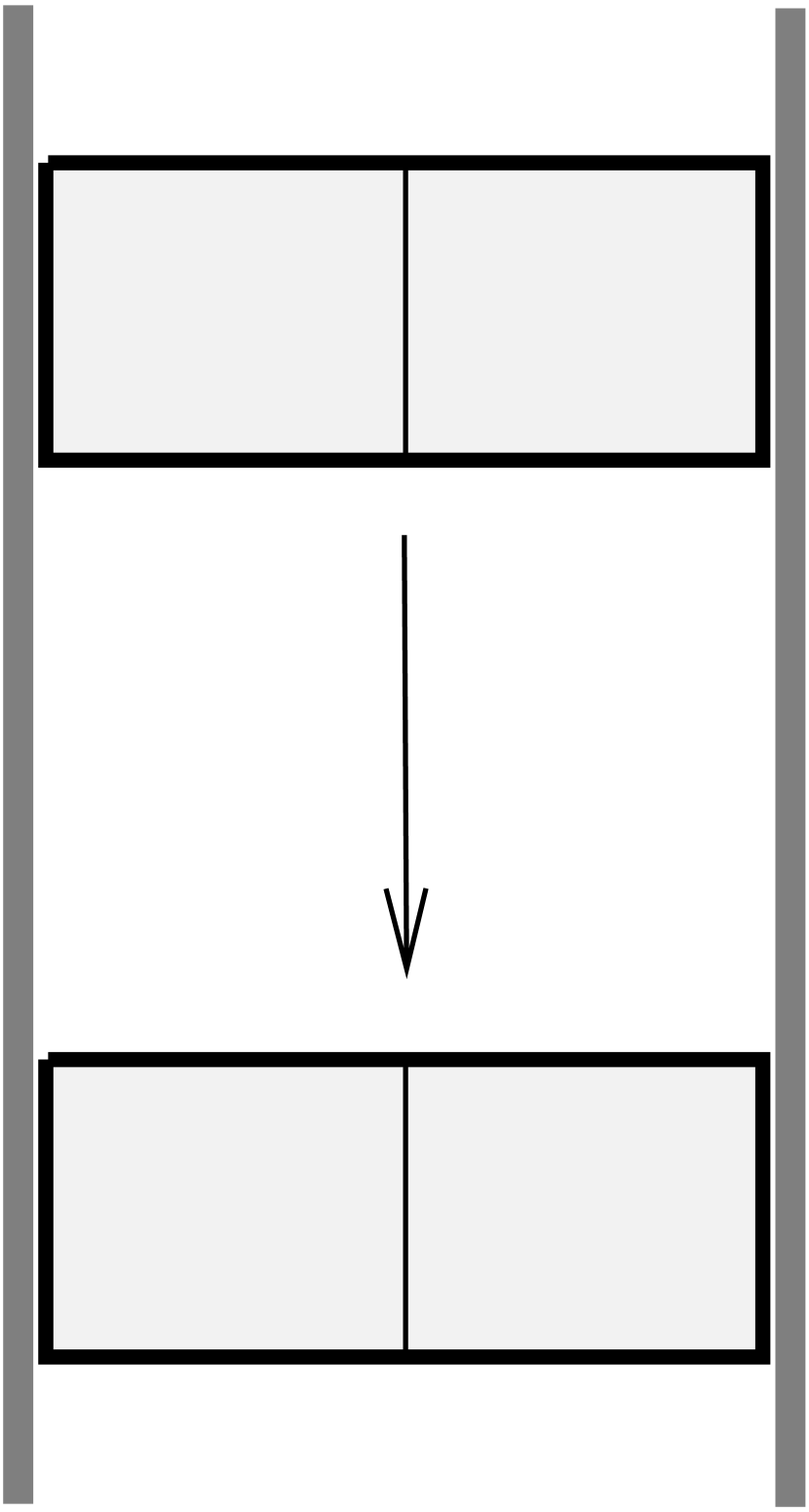
Figure 1: Lowering the box in the gravitational field with side walls attached.

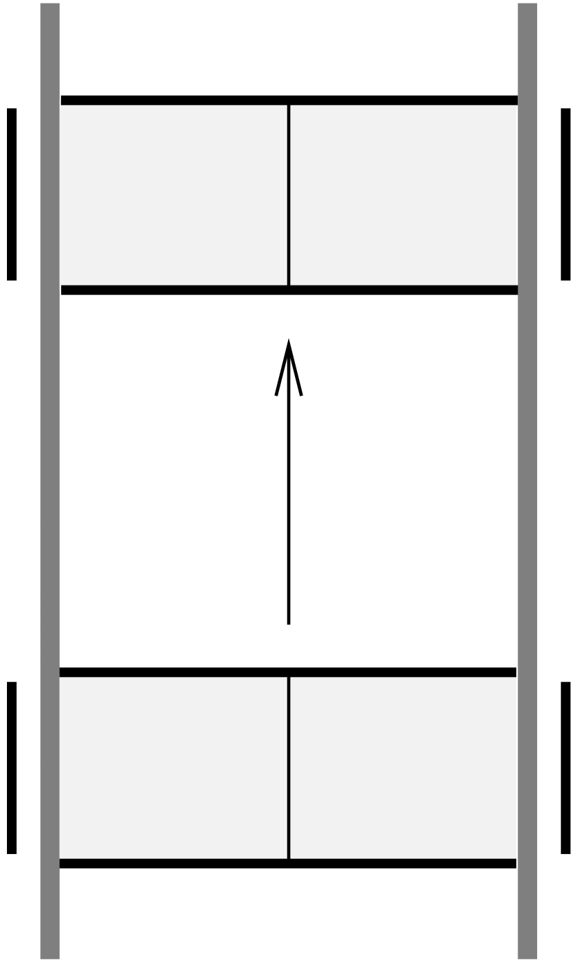
Figure 2: Raising the box in the gravitational field with side walls taken off.

Indeed, radiation plus box is a closed static system. Hence the weight of the total system is proportional to its total energy $E$, which we may pretend to be given by the radiation energy alone, since the contributions from the rest masses of the walls will cancel in the final energy balance, so that we may formally set them to zero at this point. Lowering this box by an amount $h$ in a static homogeneous gravitational field of strength $g$ results in an energy gain of $\Delta E=hgE/c^{2}$. So despite the fact that radiation has a traceless energy-momentum tensor, trapped radiation has a weight given by $E/c^{2}$. This is due to the radiation pressure which puts the walls of the trapping box under tension. Tension makes an independent contribution to weight, independent of the material that supports it. For each parallel pair of side-walls the tension is just the radiation pressure, which is one third of the energy density. So each pair of side-walls contribute $E/3c^{2}$ to the (passive) gravitational mass (over and above their rest mass, which we set to zero) in the lowering process when stressed, and zero in the raising process when unstressed. Hence, Einstein concluded, there is a net gain in energy of $2E/3c^{3}$ (there are two pairs of side walls).

But it seems that Einstein neglects the fact that, in contrast to the lowering process, during the lifting process the state of the shaft $S$ is changed. Moreover, the associated contribution to the energy balance just renders Einstein’s argument inconclusive. Indeed, when the side walls are first removed in the lower position, the walls of the shaft necessarily come under stress because they now need to provide the horizontal balancing pressures. In the raising process that stress distribution of the shaft is translated upwards. But that does cost energy, even though it is not associated with any proper transport of the material the shaft is made from. As already pointed out, stresses make their own contribution to weight, independent of the nature of the material that supports them. In particular, a redistribution of stresses in a material immersed in a gravitational field will generally makes a non-vanishing contribution to the energy balance, even if the material does not move. This is explicitly seen in the model theory discussed next.

3.2 A formally consistent model-theory for scalar gravity

We wish to construct a Poincaré-invariant theory of a scalar gravitational field, $\Phi$, coupled to matter. We will use Lagrangian methods. Regarding the Minkowski metric we use the ‘mostly minus’ convention, that is, $\eta_{\mu\nu}=\mbox{diag}(1,-1,-1,-1)$.

We start from the obvious generalization of Poisson’s equation, $\Delta\Phi=4\pi G\rho$, with the ‘Laue-scalar’ as source:

$$\square\Phi=-\kappa T\,,\quad\text{where}\quad\kappa:=4\pi G/c^{2}\,.$$ (29)

Here $\square=\eta^{\mu\nu}\partial_{\mu}\partial_{\nu}$ and $T=\eta^{\mu\nu}T_{\mu\nu}$. $T_{\mu\nu}$ is the stress-energy tensor of the matter (sign-normalization: $T_{00}=T_{0}^{0}=+$energy-density). We seek an action which makes (29) its Euler-Lagrange equation. It’s easy to guess:

$$S_{\rm field}+S_{\rm int}=\frac{1}{\kappa c^{3}}\int d^{4}x\left(\tfrac{1}{2}\partial_{\mu}\Phi\partial^{\mu}\Phi-\kappa\Phi T\right)\,.$$ (30)

where $S_{\rm field}$, given by the first term, is the action for the gravitational field and $S_{\rm int}$, given by the second term, accounts for the interaction with matter.

To this we have to add the action $S_{\rm matter}$ for the matter, which we only specify insofar as we we assume that the matter consists of a point particle of rest-mass $m_{0}$ and a ‘rest’ that needs not be specified further for our purposes here. Hence $S_{\rm matter}=S_{\rm particle}+S_{\rm rom}$ (rom = rest of matter) where

$$S_{\rm particle}=-m_{0}c^{2}\int d\tau\,.$$ (31)

The quantity $d\tau=\tfrac{1}{c}\sqrt{\eta_{\mu\nu}dz^{\mu}dz^{\nu}}$ is the proper time along the worldline of the particle. The energy-momentum tensor of the particle is given by

$$T^{\mu\nu}(x)=m_{0}c\,\int{\dot{z}}^{\mu}(\tau){\dot{z}}^{\nu}(\tau)\ \delta^{(4)}(x-z(\tau))\ d\tau\,,$$ (32)

so that the particle’s contribution to the interaction term in (30) is

$$S_{\text{int-particle}}=-m_{0}\int\Phi(z(\tau))\ d\tau\,.$$ (33)

Hence the total action can be written in the following form:

$$\begin{split}S_{\rm tot}=&-m_{0}c^{2}\int\bigl{(}1+\Phi(z(\tau))/c^{2}\bigr{)}\ d\tau\\ &+\frac{1}{\kappa c^{3}}\int d^{4}x\ \bigl{(}\tfrac{1}{2}\partial_{\mu}\Phi\partial^{\mu}\Phi-\kappa\Phi T_{\text{rom}}\bigr{)}\\ &+S_{\text{rom}}\,.\end{split}$$ (34)

By construction the field equations that follow from this action are given by (29), where the energy momentum-tensor refers to the matter without the test particle, if we treat the latter as test particle. The equations of motion for the test particle are then given by

$$\ddot{z}^{\mu} \,=\,P^{\mu\nu}\partial_{\nu}\phi\,,$$ (35a)

where $$P^{\mu\nu} \,=\,\eta^{\mu\nu}-{\dot{z}}^{\mu}{\dot{z}}^{\nu}/c^{2}$$ (35b)

and $$\phi \,=\,c^{2}\ln(1+\Phi/c^{2})\,.$$ (35c)

Two things are worth remarking at this point:

• The term $P^{\mu\nu}$ is a projector perpendicular to the timelike direction given by $\dot{z}$. It is necessary in order to avoid overdetermination. Due to $\dot{z}^{\mu}\dot{z}_{\mu}=c^{2}$ there can only be three independent equations of motion. Indeed, an equation like $\ddot{z}^{\mu}=\partial^{\mu}\phi$ immediately leads to the integrability condition $\dot{z}^{\mu}\partial_{\mu}\phi=0$, which renders this equations useless since it says that $\phi$ may not change along the worldline of the particle.

• Whereas $\Phi$ plays the analog of the Newtonian potential in the SR-adapted field equation (29), it is $\phi$ rather than $\Phi$ that plays the analog of the Newtonian equation potential in the equation of motion for a test particle. The relation between the two potential is given by (35c). We were not free to just impose an equation of motion for the test particle, in which $\phi$ in (35a) is replaced by $\Phi$. Rather, (35a) is an unambiguous consequence of the consistency requirement, according to which all forms of matter couple to gravity in the same fashion, namely via the $\Phi T$ – term in the interaction Lagrangian. From (32) via (33) this directly leads to (35).

Suppose there exists some inertial coordinate system $x^{\mu}$ with respect to which $\Phi$ (and hence $\phi$) is static, i.e. $\partial_{0}\Phi=0$, then in these coordinates (35a) is equivalent to the following 3-vector equation ($t=x^{0}$)

$$\tfrac{d^{2}}{dt^{2}}\vec{z}(t)=-\left(1-|\tfrac{d}{dt}\vec{z}(t)|^{2}/c^{2}\right)\ \vec{\nabla}\varphi(\vec{z}(t))\,.$$ (36)

From Einstein’s own recollections we know that he also arrived at an equation like (36) in an early attempt to generalize Newton’s scalar theory of gravity, but that he dismissed it for not satisfying some variant of the universality of free fall, according to which the vertical acceleration of a body should be independent of the horizontal velocity of its center of mass. In his own words:

“Dieser Satz, der auch als Satz über die Gleichheit der trägen und schweren Masse formuliert werden kann, leuchtete mir nun in seiner tiefen Bedeutung ein. Ich wunderte mich im höchsten Grade über sein Bestehen und vermutete, dass in ihm der Schlüssel für ein tieferes Verständnis der Trägheit und Gravitation liegen müsse. An seiner strengen Gültigkeit habe ich auch ohne Kenntnis des Resultates der schönen Versuche von Eötvös, die mir – wenn ich mich richtig erinnere – erst später bekannt wurden, nicht ernsthaft gezweifelt.” ([8], pp. 135–136)

Concerning this statement, at least three things seem truly remarkable:

• That Einstein would dismiss the quadratic dependence of the vertical acceleration on $v/c$, as predicted by (36), as “not in accord with the ‘old experience’ (sic!) of the universality of free fall”.

• The dependence of the vertical acceleration on the horizontal center-of-mass velocity is clearly expressed by (36). However, Einstein’s additional claim that there is also a similar dependence on the internal energy does not survive closer scrutiny. One might think at first that (36) also predicts that, for example, the gravitational acceleration of a box filled with a gas decreases with temperature, due to the increasing velocities of the gas molecules. But this arguments neglects the walls of the box which gain in stress due to the rising gas pressure. According to (29) more stress means less weight. In fact, a general argument due to Laue (1911) shows that these effects precisely cancel (see e.g. [17] for a lucid discussion).

• Einstein’s requirement that the vertical acceleration should be independent of the horizontal velocity is (for good reasons) not at all implied by the modern formulation of the (weak) equivalence principle, according to which the worldline of a freely falling test-body (without higher mass-multipole-moments and without charge and spin) is determined by its initial spacetime point and four velocity, i.e. independent of the further constitution of the test body. In contrast, Einstein’s requirement relates two motions with different initial velocities. In fact, it is badly in need of a proper interpretation to even make physical sense. Are we to require that two bodies dropped from some altitude, one with the other without horizontal initial velocity, reach the ground simultaneously? What what does ‘simultaneously’ refer to? Simultaneously in the initial rest frame of one of the two bodies? Or at the same lapse of eigentimes of the two bodies?

In passing we remark that (36) gives rise to a periastron precession of $-1/6$ times the value obtained from GR.

3.3 Energy conservation

Corresponding to Poincaré-invariance there are 10 conserved currents. In particular, the total energy $E$ relative to an inertial system is conserved. For a particle coupled to gravity it is easily calculated and consists of three contributions corresponding to the gravitational field, the particle, and the interaction-energy of particle and field:

$$E_{\scriptscriptstyle\rm gravity} \,=\,\frac{1}{2\kappa c^{2}}\int d^{3}x\ \bigl{(}(\partial_{ct}\Phi)^{2}+(\vec{\nabla}\Phi)^{2}\bigr{)}\,,$$ (37a)

$$E_{\scriptscriptstyle\rm particle} \,=\,m_{0}c^{2}\,\gamma(v)\,,$$ (37b)

$$E_{\scriptscriptstyle\rm interaction} \,=\,m_{0}\,\gamma(v)\,\Phi\bigl{(}\vec{z}(t),t\bigr{)}\,,$$ (37c)

where $v=|{d\vec{z}(t)/dt}|$ (the velocity of the particle w.r.t. the inertial system) and $\gamma(v)=1/\sqrt{1-v^{2}/c^{2}}$. This looks all very familiar.

3.4 Energy-momentum conservation in general

Let’s return to general matter models and let $\mathcal{T}^{\mu\nu}$ be the total stress-energy tensor of the gravity-matter-system. It is the sum of three contributions:

$$T_{\scriptscriptstyle\rm total}^{\mu\nu}=T_{\scriptscriptstyle\rm gravity}^{\mu\nu}+T_{\scriptscriptstyle\rm matter}^{\mu\nu}+T_{\scriptscriptstyle\rm interaction}^{\mu\nu}\,,$$ (38)

where

$$T_{\scriptscriptstyle\rm gravity}^{\mu\nu} \,=\,\frac{1}{\kappa c^{2}}\bigl{(}\partial^{\mu}\Phi\partial^{\nu}\Phi-\tfrac{1}{2}\eta^{\mu\nu}\partial_{\lambda}\Phi\partial^{\lambda}\Phi\bigr{)}\,,$$ (39a)

$$T_{\scriptscriptstyle\rm matter}^{\mu\nu} \,=\,\text{depending on matter model}\,,$$ (39b)

$$T_{\scriptscriptstyle\rm interaction}^{\mu\nu} \,=\,\eta^{\mu\nu}(\Phi/c^{2})T_{\scriptscriptstyle\rm matter}\,.$$ (39c)

Energy-momentum-conservation is expressed by

$$\partial_{\mu}{T_{\scriptscriptstyle\rm total}}^{\mu\nu}=F^{\nu}_{\scriptscriptstyle\rm external}\,,$$ (40)

where $F^{\nu}_{\scriptscriptstyle\rm external}$ is the four-force of a possible external agent. The 0-component of it (i.e. energy conservation) can be rewritten in the form

$$\mbox{external power supplied}\ =\ \frac{d}{dt}\int_{D}d^{3}x\ {T^{00}_{\scriptscriptstyle\rm total}}+\int_{\partial D}{T^{0k}_{\scriptscriptstyle\rm total}}n_{k}\ d\Omega\,.$$ (41)

If the matter system is of finite spatial extent, meaning that outside some bounded spatial region $D$ we have that $T_{\scriptscriptstyle\rm matter}^{\mu\nu}$ vanishes identically, and if we further assume that no gravitational radiation escapes to infinity, the surface integral in (41) vanishes identically. Integrating (41) over time we then get

$$\mbox{external energy supplied}\ =\ \Delta E_{\scriptscriptstyle\rm gravity}+\Delta E_{\scriptscriptstyle\rm matter}+\Delta E_{\scriptscriptstyle\rm interaction}\,,$$ (42)

with

$$E_{\scriptscriptstyle\rm interaction}=\int_{D}d^{3}x\ (\Phi/c^{2})T_{\scriptscriptstyle\rm matter}\,,$$ (43)

and where $\Delta(\mbox{something})$ denotes the difference between the initial and final value of ‘something’. If we apply this to a process that leaves the internal energies of the gravitational field and the matter system unchanged, for example a processes where the matter system, or at least the relevant parts of it, are rigidly moved in the gravitational field, like in Einstein’s Gedankenexperiment of the ‘radiation-shaft-system’, we get

$$\mbox{external energy supplied}\ =\ \Delta\left\{\int_{D}d^{3}x\ (\Phi/c^{2})T_{\scriptscriptstyle\rm matter}\right\}\,.$$ (44)

Now my understanding of what a valid claim of energy non-conservation would be, is to show that this equation can be violated, granted the hypotheses under which it was derived. This is not what Einstein did (compare Conclusions).

If the matter system stretches out to infinity and conducts energy and momentum to infinity, than the surface term that was neglected above gives a non-zero contribution that must be included in (44). Then a proof of violation of energy conservation must disprove this modified equation. (Energy conduction to infinity as such is not in any disagreement with energy conservation; you have to prove that they do not balance in the form predicted by the theory.)

3.5 Conclusion

For the discussion of Einstein’s Gedankenexperiment the term (43) is the relevant one. It accounts for the weight of stress. Pulling up a radiation-filled box inside a shaft also moves up the stresses in the shaft walls that must act sideways to balance the radiation pressure. This lifting of stresses to higher gravitational potential costs energy, according to the theory presented here. This energy was neglected by Einstein, apparently because it is not associated with a transport of matter. He included it in the lowering phase, where the side-walls of the box are attached to the box and move with it, but neglected them in the raising phase, where the side walls are those of the shaft, which do not move. But as far as the ‘weight of stresses’ is concerned, this difference is irrelevant. What (43) tells us is that raising stresses in an ambient gravitational potential costs energy, irrespectively of whether it is associated with an actual transport of the stressed matter or not. This would be just the same for the transport of heat in a heat conducting material. Raising the heat distribution against the gravitational field costs energy, even if the material itself does not move.

I conclude that Einstein’s argument is not convincing. Clearly this is not meant to give any scientific support to scalar theories of gravity (as opposed to GR), which we know are ruled out by experiment. For example, as already mentioned above, the model theory discussed here gives the wrong amount (even the wrong sign) for the perihelion shift of Mercury, namely $-1/6$ times Einstein’s value. Moreover, theories in which the gravitational field couples to matter via its trace of the energy-momentum tensor predict a vanishing global deflection of light. But what is not the case is that scalar theories are intrinsically inconsistent, as apparently suggested by Einstein. For Einstein this argument might have appeared as a convenient physical way to rule out scalar theories, whose primary deficiency he saw, however, in the lack of being generally covariant.

Acknowledgements

I thank Jürgen Ehlers for remarks and discussions.

References

- [1] Ralph Abraham and Jerrold E. Marsden. Foundations of Mechanics. The Benjamin/Cummings Publishing Company, Reading, Massachusetts, second edition, 1978.
- [2] James L. Anderson. Relativity principles and the role of coordinates in physics. In Hong-Yee Chiu and William F. Hoffmann, editors, Gravitation and Relativity, pages 175–194. W.A. Benjamin, Inc., New York and Amsterdam, 1964.
- [3] James L. Anderson. Principles of Relativity Physics. Academic Press, New York, 1967.
- [4] Julian Barbour. On general covariance and best matching. In Craig Callender and Nick Huggett, editors, Physics Meets Philosophy at the Planck Scale – Contemporary Theories in Quantum Gravity, pages 199–212. Cambridge University Press, Cambridge (England), 2001.
- [5] Otto Bergmann. Scalar field theory as a theory of gravitation. I. American Journal of Physics, 24(1):38–42, 1956.
- [6] Elie Cartan. Sur les varietes a connexion affine et la théorie de la relativité généralisée. Annales Scientifiques de l’École Normale Supérieure, 40:325–412, 1923.
- [7] Elie Cartan. Sur les varietes a connexion affine et la théorie de la relativité généralisée. Annales Scientifiques de l’École Normale Supérieure, 41:1–15, 1924.
- [8] Albert Einstein. Mein Weltbild. Ullstein Verlag, Berlin, 1977.
- [9] Michael Friedman. Relativity principles, absolute objects and symmetry groups. In Patrick Suppes, editor, Space, Time and Geometry, pages 296–320, Dordrecht, Holland, 1973. D. Reidel Publishing Company.
- [10] Michael Friedman. Foundations of Space-Time Theories. Princeton University Press, Princeton, New Jersey, 1983.
- [11] K. Friedrichs. Eine invariante Formulierung des Newtonschen Gravitationsgesetzes und des Grenzüberganges vom Einsteinschen zum Newtonschen Gesetz. Mathematische Analen, 98:566–575, 1927.
- [12] A.L. Harvey. Brief review of lorentz-covariant scalar theories of gravitation. American Journal of Physics, 33(6):449–460, 1965.
- [13] Roger Jones. The special and general principles of relativity. In P. Barker and C.G. Shugart, editors, After Einstein, pages 159–173, Memphis, USA, 1981. Memphis State University Press.
- [14] Erich Kretschmann. Über den physikalischen Sinn der Relativitätspostulate, A. Einsteins neue und seine ursprüngliche Relativitätstheorie. Annalen der Physik, 53:575–614, 1917.
- [15] Jürgen Moser. On the volume elements on a manifold. Transactions of the American Mathematical Society, 120(2):286–294, 1965.
- [16] John Norton. Einstein, Nordström and the early demise of scalar Lorentz-covariant theories of gravitation. Archive for the History of Exact Sciences, 45:17–94, 1992.
- [17] John Norton. Einstein and Nordström: Some lesser known thought experiments in gravitation. In John Earman, Michel Janssen, and John Norton, editors, The Attraction of Gravitation: New Studies in History of General Relativity, pages 3–29, Boston, MA, 1993. Birkäuser Verlag.
- [18] John Norton. General covariance and the foundations of general relativity: Eight decades of dispute. Reports of Progress in Physics, 56:791–858, 1993.
- [19] John Norton. General covariance, gauge theories and the Kretschmann objection. In Katherine Brading and Elena Castellani, editors, Symmetries in Physics: Philosophical Reflections, pages 110–123. Cambridge University Press, Cambridge, UK, 2003.
- [20] Wolfgang Pauli. Theory of Relativity. Dover Publications, Inc., New York, 1981. Unabridged and unaltered republication of the english translation by G. Field that was first published in 1958 by Pergamon Press.
- [21] Wolfgang Pauli. Relativitätstheorie. Springer Verlag, Berlin, 2000. Reprint of the original ‘Encyclopädie-Artikel’ from 1921 with various additions, including Pauli’s own supplementary notes from 1956. Edited and annotated by Domenico Giulini.
- [22] Lee Smolin. The case for background independence. www.arxiv.org/abs/hep-th/0507235.
- [23] Rafael Sorkin. An example relevant to the Kretschmann-Einstein debate. Modern Physics Letters A, 17(11):695–700, 2002.
- [24] John Stachel et al., editors. The Collected Papers of Albert Einstein, Vols. 1-9. Princeton University Press, Princeton, New Jersey, 1987-2005.
- [25] Norbert Straumann. General Relativity. Springer Verlag, Berlin, 2004.
- [26] Max von Laue. Die Nordströmsche Gravitationstheorie. Jahrbuch der Radioaktivität und Elektronik, 14(3):263–313, 1917.