Stability analysis of sonic horizons in Bose-Einstein condensates

Abstract

We examine the linear stability of various configurations in Bose-Einstein condensates with sonic horizons. These configurations are chosen in analogy with gravitational systems with a black hole horizon, a white hole horizon and a combination of both. We discuss the role of different boundary conditions in this stability analysis, paying special attention to their meaning in gravitational terms. We highlight that the stability of a given configuration, not only depends on its specific geometry, but especially on these boundary conditions. Under boundary conditions directly extrapolated from those in standard General Relativity, black hole configurations, white hole configurations and the combination of both into a black hole–white hole configuration are shown to be stable. However, we show that under other (less stringent) boundary conditions, configurations with a single black hole horizon remain stable, whereas white hole and black hole–white hole configurations develop instabilities associated to the presence of the sonic horizons.

I Introduction

It is widely expected that underneath the general relativity description of gravitational phenomena there is a deeper layer in which quantum physics plays an important role. However, at this stage we don’t have enough intertwined theoretical and observational knowledge to know how an appropriate description of what underlies gravity is or should be. Moreover, starting from structurally-complete quantum theories of gravity, it could still be very difficult to extract the specific way in which the first “quantum” modifications to classical general relativity might show up (this happens for example within the Loop Quantum Gravity approach LQG ).

Analogue models of General Relativity (GR) analogue-book ; review provide specific and clear examples in which effective spacetime structures ultimately emerge from (non-relativistic) quantum many-body systems. For certain (semiclassical) configurations and low levels of resolution, one can appropriately describe the physical behaviour of the system by means of a classical (or quantum) field theory in a curved (Lorentzian) background geometry. However, when one probes the system with higher and higher resolution, the geometrical structure progressively dissolves into a purely quantum regime barcelo-bec . Therefore, although analogue models cannot be considered at this stage complete models of quantum gravity (they do not lead to the Einstein equations in any regime or approximation), they provide specific and tractable models that reproduce many aspects of the overall scenario expected in the realm of real gravity.

The main objective of this and similar studies is to obtain specific indications about the type of deviations from the GR behaviour to be expected when quantum gravitational effects become important. All, under the assumption that the underlying structure to GR is somewhat similar to that in condensed matter systems. In particular, in this paper we are interested in the behaviour of gravity-like configurations containing horizons within Bose–Einstein condensates (BECs). (See, e.g., Refs. dalfovo ; castin ; ketterle and barcelo-bec ; sonicBH1 ; sonicBH2 for reviews on BECs and for their usefulness as analogue models respectively). A nice feature of these systems is that their theoretical description in terms of the Gross-Pitaevskii (GP) equation can be interpreted as incorporating, from the start, the first “quantum” corrections to the behaviour of the system. Linear perturbations over a background BEC configuration satisfy an equation which is a standard wave equation over a curved effective spacetime plus corrections containing $\hbar$. These corrections cause the dispersion relations in BEC to be “superluminal” (strictly speaking, supersonic): some perturbations can travel faster than the speed of sound in the system. The effects of these corrections in the linearized dynamical evolution of a configuration are especially relevant in the presence of horizons as their one-way-membrane nature simply disappears. This is in tune with the idea that a horizon can serve as a magnifying glass of the physics at high energies (see, e.g., Ref. Padmanabhan:1998vr ).

The specific objective of this paper is to analyze the dynamical behaviour of (effectively) one-dimensional BECs with density and velocity profiles containing one or two sonic horizons. In particular, we search for the presence of dynamical instabilities and analyze how their existence is related to the occurrence of these horizons. The stability analysis presented in Ref. sonicBH2 for black hole-like configurations with fluid sinks in their interior, concluded that these configurations were intrinsically unstable. However, the WKB analysis of the stability of horizons in Ref. leonhardt suggested that black hole horizons might well be stable, while configurations with white hole horizons seem to posses unstable modes. Regarding configurations in which a black hole horizon is connected with a white hole horizon in a straight line, the analysis presented in Ref. jacobson concluded, also within a WKB approximation, that these configurations were intrinsically unstable, producing a so-called “black hole laser”. However, when the white hole horizon is connected back to the black hole horizon to produce a ring, it was found that these configurations can be stable or unstable depending on their specific form sonicBH1 ; sonicBH2 . This suggests that periodic boundary conditions can eliminate some of the instabilities associated with the black hole laser.

In this paper we will try to shed some light on all of these issues and clear up some of the apparent contradictions. To simplify matters, we will consider one-dimensional profiles that are piecewise uniform with either one or two step-like discontinuities. As has been discussed in Ref. sonicBH2 , in terms of dynamical (in)stability, there seems to be no crucial qualitative difference between the present case and a profile with smooth transitions between regions with an (asymptotically) uniform density distribution. Therefore the idealized case that we consider here should contain all the essential information relevant to more complicated profiles as well. The specific way to examine the kind of instability we are interested in, consists basically in seeking whether, under appropriate boundary conditions, there are complex eigenfrequencies of the system which lead to an exponential increase with time of the associated perturbations, i.e. a dynamical instability. Throughout the paper we will use a language and notation as close to GR as possible. In particular, we will use boundary conditions similar to those imposed in the standard quasi-normal mode analysis of black holes in GR quasi-normal-modes . One of the main results of our analysis is to highlight the fundamental importance of the boundary conditions in determining whether a configuration is stable or unstable.

The structure of this paper is as follows. In the next section we will review the basic ingredients of gravitational analogies in BECs. At the same time, we will set up the conceptual framework for our discussion, based on a parametrization well adapted for an acoustic interpretation (a brief comparison with the Bogoliubov representation is presented in appendix B). Section III contains a detailed formulation of our specific problem. This includes the mode expansion in uniform sections, a derivation of the matching conditions at each discontinuity and a discussion of the various boundary conditions to be applied. Then, in section IV we proceed case by case, analyzing different situations and presenting the results we have obtained for each of them. This includes a brief description of the numerical algorithm we have used. Finally, in section V we discuss our results, compare them with other results available in the literature, and draw some conclusions.

II Preliminaries

In second quantization, a dilute gas of interacting bosons can be described by a quantum field $\widehat{\Psi}$ satisfying the equation

$${\rm i}\hbar\;\frac{\partial}{\partial t}{\widehat{\Psi}}=\left(-{\hbar^{2}\over 2m}\nabla^{2}+V_{\rm ext}({\mathbf{x}})+\text{\sl g}{\widehat{\Psi}}^{\dagger}{\widehat{\Psi}}\right){\widehat{\Psi}},$$ (1)

where $m$ is the boson mass, $V_{\text{ext}}$ the external potential and g the coupling constant which is related to the corresponding scattering length $a$ through $\text{\sl g}={4\pi\hbar^{2}a/m}$. In this manner all quantum effects can, in principle, be taken into account. Once the Bose-Einstein condensation has taken place, the quantum field can be separated into a macroscopic wave function $\psi$ (the corresponding order parameter) and a field operator $\widehat{\varphi}$ describing quantum fluctuations over it: ${\widehat{\Psi}}=\psi+{\widehat{\varphi}}$. The macroscopic wave function satisfies the Gross-Pitaevskii (GP) equation

$${\rm i}\hbar\;\frac{\partial}{\partial t}\psi(t,{\mathbf{x}})=\left(-{\hbar^{2}\over 2m}\nabla^{2}+V_{\rm ext}({\mathbf{x}})+\text{\sl g}\;|\psi|^{2}\right)\psi(t,{\mathbf{x}}),$$ (2)

while for the linear quantum perturbation we have the Bogoliubov equation

$${\rm i}\hbar\;\frac{\partial}{\partial t}{\widehat{\varphi}}=\left(-{\hbar^{2}\over 2m}\nabla^{2}+V_{\rm ext}({\mathbf{x}})+\text{\sl g}\;2|\psi|^{2}\right){\widehat{\varphi}}+\text{\sl g}\;\psi^{2}\;{\widehat{\varphi}}^{\dagger}.$$ (3)

Adopting the Madelung representation for the order parameter

$$\psi=\sqrt{n}e^{{\rm i}\theta/\hbar}e^{-{\rm i}\mu t/\hbar}$$ (4)

(here $n$ is the condensate density, $\mu$ the chemical potential and $\theta$ a phase factor which is related to the velocity potential), and substituting in (2) we arrive at

$$\partial_{t}n =-{1\over m}\nabla\cdot(n\nabla\theta),$$ (5a)

$$\partial_{t}\theta =-{1\over 2m}(\nabla\theta)^{2}-\text{\sl g}\;n-V_{\text{ext}}-\mu-V_{\text{quantum}},$$ (5b)

where the so-called “quantum potential” is defined as

$$V_{\text{quantum}}=-{\hbar^{2}\over 2m}{\nabla^{2}\sqrt{n}\over\sqrt{n}}.$$ (6)

In most situations the quantum potential in Eq. (5b) can be neglected (see below). The resulting equations (5a) and (5b) are then equivalent to the continuity equation and the Bernoulli equation for a classical fluid. In this case, it is well known that the propagation of acoustic waves in the system can be described by means of an effective metric, thus providing the analogy with the propagation of fields in curved spacetimes Unruh:1980cg ; visser97 . Given a background configuration ($n_{0}$ and $\theta_{0}$), this metric can be written as

$$(g_{\mu\nu})=\frac{m}{\text{\sl g}}c\begin{pmatrix}v^{2}-c^{2}&&-\mathbf{v}^{\text{T}}\\ -\mathbf{v}&&\mathbf{\openone}\end{pmatrix},$$ (7)

where $c^{2}\equiv\text{\sl g}n_{0}/m$ and $\mathbf{v}\equiv\nabla\theta_{0}/m$. These magnitudes, $c$ and $\mathbf{v}$, represent the local velocity of sound and the local velocity of the fluid flow respectively.

The functions $c(t,{\mathbf{x}})$ and $\mathbf{v}(t,{\mathbf{x}})$ completely characterize the acoustic metric. In GR any metric has to be obtained by solving the Einstein equations. Here, however, the magnitudes $c(t,{\mathbf{x}})$ and $\mathbf{v}(t,{\mathbf{x}})$, and so the acoustic metric, are those satisfying the continuity and Bernoulli equations of hydrodynamics [Eqs. (5) without the quantum potential]. Thus, these equations play a role analogous to the vacuum Einstein equations in GR. Of course, at the global non-linear level these equations are completely different from the real Einstein equations. But their way of acting when linearized around a background solution captures the essence of a proper linearized GR behaviour.

There exist, however, situations in which the quantum potential in Eq. (5) cannot be neglected. This is evidently the case if the characteristic length of the spatial variations of the condensate density is much smaller than the so-called healing length: $\xi\equiv\hbar/(mc)$. But this case is not the only one. To illustrate this point, let us consider the dispersion law obtained for a homogeneous BEC (see below):

$$(\omega-vk)^{2}=c^{2}k^{2}+{1\over 4}c^{2}\xi^{2}k^{4}.$$ (8)

This is a “superluminally modified” dispersion relation due to the presence of the term with $k^{4}$. For $\xi k\ll 1$ we can rewrite this expression as

$$\omega=\left(v\pm c\sqrt{1+{1\over 4}\xi^{2}k^{2}}\right)k\simeq(v\pm c)k+{1\over 8}c\xi^{2}k^{3}+\mathcal{O}(\xi^{4}k^{5}).$$ (9)

Here we clearly see that the (relative) importance of the term $\propto k^{3}$, given by ${c\over 8(v\pm c)}\xi^{2}k^{2}$, depends not only on the ratio between the corresponding wavelength and the healing length, $\xi k$, but also on the specific features of the background magnitudes [note that the factor $c/(v\pm c)$ may be quite large]. In other words, the smallness of the corresponding wavelength is a necessary condition in order to neglect the contribution of the quantum potential, but it is not a sufficient condition. One has to bear this issue in mind, especially when the system possesses horizons (i.e. points at which $c^{2}=v^{2}$).

Summarizing, there are background configurations which, when probed with sufficiently large wavelengths, act as if they were effective Lorentzian geometries. But there are other configurations for which this geometrical interpretation fails, irrespective of the probing wavelength. The latter situation occurs when there are horizons in the configuration: strictly speaking, we cannot talk about an “effective Lorentzian geometry” in the regions surrounding these horizons.

Without forgetting this subtlety, we will continue to call (7) the “effective metric” in the system, even when analyzing the full GP equation. Then, we can consider the equations (5) to play the role of some sort of semiclassical vacuum Einstein equations. Their treatment is classical, but they incorporate corrections containing $\hbar$. Therefore, BECs’ standard treatment based on the GP equation provides an example of a way of incorporating quantum corrections to the dynamics of a system without recurring to the standard procedures of back-reaction. Again, although at the global non-linear level these equations bear no relationship whatsoever with any sort of ”semiclassical” Einstein equations, at the linear level, that is, in terms of linear tendencies of departing from a given configuration, equations (5) encode the essence of the linearized GR behaviour (a Lorentzian wave equation in a curved background), semiclassically modified to incorporate a superluminal dispersion term, as we have already discussed.

We will now proceed to describe the details of our specific calculations.

III Dynamical analysis

As a first step in our calculations, let us linearize the Eqs. (5). Let us write

$$n({\mathbf{x}},t) =n_{0}({\mathbf{x}})+\text{\sl g}^{-1}\widetilde{n}_{1}({\mathbf{x}},t),$$ (10a)

$$\theta({\mathbf{x}},t) =\theta_{0}({\mathbf{x}})+\theta_{1}({\mathbf{x}},t),$$ (10b)

where $\widetilde{n}_{1}$ and $\theta_{1}$ are small perturbations of the density and phase of the BEC. The Eqs. (5) then separate into two time-independent equations for the background,

$$0 =-\nabla\cdot(c^{2}\mathbf{v}),$$ (11a)

$$0 =-{1\over 2}m\mathbf{v}^{2}-mc^{2}-V_{\text{ext}}-\mu+{\hbar^{2}\over 2m}{\nabla^{2}c\over c},$$ (11b)

plus two time-dependent equations for the perturbations,

$$\partial_{t}\widetilde{n}_{1} =-\nabla\cdot\left(\widetilde{n}_{1}\mathbf{v}+c^{2}\nabla\theta_{1}\right),$$ (12a)

$$\partial_{t}\theta_{1} =-\mathbf{v}\cdot\nabla\theta_{1}-\widetilde{n}_{1}+{1\over 4}\xi^{2}\nabla\cdot\left[c^{2}\nabla\left({\widetilde{n}_{1}\over c^{2}}\right)\right].$$ (12b)

We will restrict ourselves to work in (1+1) dimensions. This means that we consider perturbations propagating in a condensate in such a way that the transverse degrees of freedom are effectively frozen. In other words, the only allowed motions of both the perturbations and the condensate itself are along the $x$-axis.

We will examine two types of one-dimensional background profiles. The first type consists of two regions each with a uniform density and velocity, connected through a step-like discontinuity. The second type of profiles consists of three homogeneous regions, and hence two discontinuities. We wish to know whether these profiles do or do not present dynamical instabilities. The underlying question is the relation between the presence of horizons and these dynamical instabilities. At each discontinuity, matching conditions apply that connect the magnitudes describing the condensate at both sides of the discontinuity. Furthermore, we need a set of boundary conditions, which determine what happens at the far ends of the condensate. Finally, in the uniform sections of the condensate, the regime can either be subsonic or supersonic, and of course there will be an acoustic horizon at each transition between a subsonic and a supersonic region. All these elements determine the characteristics of the system, and hence its eigenfrequencies.

We will now describe these elements one by one in detail.

III.1 Plane-wave expansion in uniform regions

In order to study the dynamics of the system, let us first consider a region in which the condensate is homogeneous (with $c$ and $v$ constant), and seek for solutions of Eqs. (12) in the form of plane waves:

$$\widetilde{n}_{1}(x,t) =Ae^{i(kx-\omega)t},$$ (13a)

$$\theta_{1}(x,t) =Be^{i(kx-\omega)t},$$ (13b)

where $A$ and $B$ are constant amplitude factors. Our aim is to elucidate about the possible instabilities of the system, so the frequency $\omega$ and the wavevector $k$ in these expressions will be considered as complex hereafter [the existence of solutions with Im$(\omega)>0$ would indicate the instability of the system]. Substituting into Eqs. (12) we find

$$\begin{pmatrix}i(\omega-vk)&&c^{2}k^{2}\\ \\ 1+{1\over 4}\xi^{2}k^{2}&&-i(\omega-vk)\end{pmatrix}\begin{pmatrix}A\\ \\ B\end{pmatrix}=0.$$ (14)

For a non-trivial solution to exist, the determinant of the above matrix must vanish. This condition gives the dispersion law (8) and since this is a fourth order polynomial in $k$, its roots will, in general, give four independent solutions for the equations of motion in the form (13).

III.2 Matching conditions at a discontinuity

Let us take $x=0$ to be a point of discontinuity. The values of $v$ and $c$ both undergo a finite jump when crossing this point. These jumps have to satisfy the background constraint $vc^{2}=\text{const}$ [see Eq. (11a)]. The solutions of Eqs. (12) in the regions $x<0$ and $x>0$ have the form of plane waves which are then subject to matching conditions at $x=0$. It is not difficult to see that $\theta_{1}$ has to be continuous at the jump but with a discontinuous derivative, while the function $\widetilde{n}_{1}$ has to undergo a finite jump. The exact conditions can be obtained by integrating Eqs. (12) about an infinitesimal interval containing the point $x=0$. This results in the following four independent, generally valid matching conditions:

$$[\theta_{1}]=0,\qquad[v\widetilde{n}_{1}+c^{2}\partial_{x}\theta_{1}]=0,$$ (15a)

$$\left[{\widetilde{n}_{1}\over c^{2}}\right]=0,\qquad\left[c^{2}\partial_{x}\left({\widetilde{n}_{1}\over c^{2}}\right)\right]=0.$$ (15b)

The square brackets in these expressions denote, for instance, $[\theta_{1}]=\left.\theta_{1}\right|_{x=0^{+}}-\left.\theta_{1}\right|_{x=0^{-}}$. We can simplify the second condition in Eq.(15a) to $[c^{2}\partial_{x}\theta_{1}]=0$ by noting that $[v\widetilde{n}_{1}]=0$ because of the background continuity equation (11a), while for our choice of a homogeneous background the last condition becomes simply $[\partial_{x}\widetilde{n}_{1}]=0$.

For a given frequency $\omega$, the general solution of Eqs. (12) can be written as

$$\widetilde{n}_{1}=\begin{cases}\displaystyle\sum_{j=1}^{4}A_{j}e^{i(k_{j}x-\omega t)}&(x<0),\\ \displaystyle\sum_{j=5}^{8}A_{j}e^{i(k_{j}x-\omega t)}&(x>0),\end{cases}\qquad\qquad\theta_{1}=\begin{cases}\displaystyle\sum_{j=1}^{4}A_{j}{\omega-v_{\text{L}}k_{j}\over ic^{2}_{\text{L}}k^{2}_{j}}e^{i(k_{j}x-\omega t)}&(x<0),\\ \displaystyle\sum_{j=5}^{8}A_{j}{\omega-v_{\text{R}}k_{j}\over ic^{2}_{\text{R}}k^{2}_{j}}e^{i(k_{j}x-\omega t)}&(x>0),\end{cases}$$ (16)

where $\{k_{j}\}$ are the roots of the corresponding dispersion equations (four roots for each homogeneous region), and the constants $A_{j}$ have to be such that the matching conditions (15) are satisfied. The subscripts $L$ and $R$ indicate the values of $c$ and $v$ in the left-hand-side (lhs) and the right-hand-side (rhs) region respectively. We can write down these conditions in matrix form $\Lambda_{ij}A_{j}=0$, where

$$\left(\Lambda_{ij}\right)=\begin{pmatrix}{\omega-v_{\text{L}}k_{1}\over c^{2}_{\text{L}}k^{2}_{1}}&{\omega-v_{\text{L}}k_{2}\over c^{2}_{\text{L}}k^{2}_{2}}&{\omega-v_{\text{L}}k_{3}\over c^{2}_{\text{L}}k^{2}_{3}}&{\omega-v_{\text{L}}k_{4}\over c^{2}_{\text{L}}k^{2}_{4}}&-{\omega-v_{\text{R}}k_{5}\over c^{2}_{\text{R}}k^{2}_{5}}&-{\omega-v_{\text{R}}k_{6}\over c^{2}_{\text{R}}k^{2}_{6}}&-{\omega-v_{\text{R}}k_{7}\over c^{2}_{\text{R}}k^{2}_{7}}&-{\omega-v_{\text{R}}k_{8}\over c^{2}_{\text{R}}k^{2}_{8}}\\ \\ {\omega\over k_{1}}&{\omega\over k_{2}}&{\omega\over k_{3}}&{\omega\over k_{4}}&-{\omega\over k_{5}}&-{\omega\over k_{6}}&-{\omega\over k_{7}}&-{\omega\over k_{8}}\\ \\ {1\over c^{2}_{\text{L}}}&{1\over c^{2}_{\text{L}}}&{1\over c^{2}_{\text{L}}}&{1\over c^{2}_{\text{L}}}&-{1\over c^{2}_{\text{R}}}&-{1\over c^{2}_{\text{R}}}&-{1\over c^{2}_{\text{R}}}&-{1\over c^{2}_{\text{R}}}&\\ \\ k_{1}&k_{2}&k_{3}&k_{4}&-k_{5}&-k_{6}&-k_{7}&-k_{8}&\\ \end{pmatrix}.$$ (17)

Furthermore, these conditions have to be complemented with conditions at the boundaries of the system and then we will obtain the solution of a particular problem.

III.3 Boundary conditions

In order to extract the possible intrinsic instabilities of a BEC configuration, we have to analyze whether there are linear mode solutions with positive $\text{Im}(\omega)$ that satisfy outgoing boundary conditions. By “outgoing” boundary conditions we mean that the group velocity is directed outwards (toward the boundaries of the system). The group velocity for a particular $k$-mode is defined as

$$v_{g}\equiv\text{Re}\left(\frac{d\omega}{dk}\right)=\text{Re}\left(\frac{c^{2}k+{1\over 2}\xi^{2}c^{2}k^{3}}{\omega-vk}+v\right),$$ (18)

where we have used the dispersion relation (8). The physical idea behind this outgoing boundary condition is that only disrupting disturbances originated inside the system can be called instabilities.

To illustrate this assertion, let us look at the classical linear stability analysis of a Schwarzschild black hole in GR. When considering outgoing boundary conditions both at the horizon and in the asymptotic region at infinity quasi-normal-modes , only negative $\text{Im}(\omega)$ modes (the quasi-normal modes) are found, and thus the black hole configuration is stable. If the presence of ingoing waves at infinity were allowed, there would also exist positive $\text{Im}(\omega)$ solutions. In other words, the Schwarzschild solution in GR is stable when considering only internal rearrangements of the configuration. If instead the black hole were allowed to absorb more and more energy coming from infinity, its configuration would continuously change and appear to be unstable.

The introduction of modified dispersion relations adds an important difference with respect to the traditional boundary conditions used in linearized stability analysis in GR. Consider for example a black hole configuration. In a BEC black hole, one boundary is the standard asymptotic region, just like in GR. For an acoustic (quadratic) dispersion relation, nothing can escape from the interior of a sonic black hole (the acoustic behaviour is analogous to linearized GR). But due to the superluminal corrections, information from the interior of the acoustic black hole can escape through the horizon and affect its exterior. Therefore, since we are taking this permeability of the horizon into consideration, the other boundary is not the black hole horizon itself (usually described in GR by an infinite value of the “tortoise” coordinate; see for example quasi-normal-modes ), but the internal singularity. The outgoing boundary condition at such a singularity reflects the fact that no information can escape from it.

There is another complication that deserves some attention. In the case of a phononic dispersion relation, the signs of $v_{g}\equiv v\pm c$ and $\text{Im}(k)\equiv(v\pm c)\text{Im}(\omega)$ coincide for $\text{Im}(\omega)>0$. For example, in an asymptotic $x\to+\infty$ subsonic region, an outgoing $k$-mode has $v_{g}>0$, so that $\text{Im}(k)>0$ and, therefore, the mode is damped towards this infinity (giving a finite contribution to its norm). Owing to this fact, in the linear stability analysis of black hole configurations, it is usual to assume that stable modes correspond to non-normalizable perturbations (think of the standard quasi-normal modes), while unstable modes correspond to normalizable perturbations.

When considering modified dispersion relations, however, this association no longer holds. In particular, with the BEC dispersion relation, in an asymptotic $x\to+\infty$ region, among the unstable ($\text{Im}(\omega)>0$) outgoing ($v_{g}>0$) $k$-modes, there are modes with $\text{Im}(k)>0$ as well as modes with $\text{Im}(k)<0$. An appropriate interpretation of these two possibilities seems to be the following. The unstable outgoing modes that are convergent at infinity (those with $\text{Im}(k)>0$) are associated with perturbations of the system that are initiated in an internal compact region of the system. Unstable outgoing modes that are divergent at infinity are associated with initial perturbations acting also at the boundary at infinity itself.

Take for example a black hole-like configuration of the form described in Fig. 1. The right asymptotic region, which can be interpreted as containing a “source” of BEC gas in our analogue model, simulates the asymptotic infinity outside the black hole in GR. The convergence condition at the rhs then implies that the perturbations are not allowed to affect this asymptotic infinity initially. However, for the left asymptotic region, this condition is less obvious. In our BEC configuration, this left asymptotic region can be seen as representing a “sink”. It corresponds to the GR singularity of a gravitational black hole. The fact that in GR this singularity is situated at a finite distance (strictly speaking, at a finite amount of proper time) from the horizon, indicates that it might be sensible to allow the perturbations to affect this left asymptotic region from the start. We will therefore consider two possibilities for the boundary condition at $x\rightarrow-\infty$. (a) Either we impose convergence in both asymptotic regions, thereby eliminating the possibility that perturbations have an immediate initial effect on the sink, or (b) we allow the perturbations to affect the sink right from the start, i.e. we don’t impose convergence at the left asymptotic region. The option of imposing the convergence at the left asymptotic region could be interpreted as excluding the influence of the singularity on the stability of the system. In other words, condition (b) would then be equivalent to examining the stability due to the combined influence of the horizon and the singularity, while under condition (a) only the stability of the horizon would be taken into account.

As a final note to this discussion, since we are interested in the analogy with gravity, we have assumed an infinite system at the rhs. In a realistic condensate other boundary conditions could apply, for example taking into account the reflection at the ends of the condensate (see e.g. sonicBH1 ; sonicBH2 ).

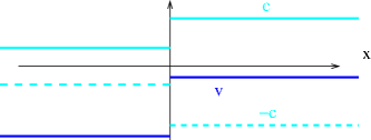
Figure 1: Flow and sound velocity profiles with step-like discontinuities simulating a black hole-like configuration. The negative value of $v$ indicates that the fluid is left-moving. At the rhs, the fluid is subsonic since $c>\lvert v\rvert$. At the lhs it has become supersonic. At $x=0$, there is a sonic horizon.

IV Case by case analysis and results

We will now briefly describe the general calculation method which we have used, and then discuss case by case the specific configurations we have analyzed.

IV.1 Numerical method

We first consider background flows and sound velocity profiles with one discontinuity. We will always assume left-moving flows.

We are seeking for possible solutions of the linearized Eqs. (12) with $\text{Im}(\omega)>0$. We use the following numerical method:

1. For each frequency $\omega$ in a grid covering an appropriate region of the upper-half complex plane, we calculate its associated $k$-roots [by solving the dispersion relation (8)] and their respective group velocities (18) at both the lhs and the rhs of the configuration.

2. We then take the four equations $\Lambda_{ij}A_{j}=0$, where $\Lambda$ is the $4\times 8$ matrix (17) determined by the matching conditions at the discontinuity. For each mode $k_{j}$ that does not satisfy the boundary conditions in the relevant asymptotic region, we add an equation of the form $A_{j}=0$. Thus we have a total set of equations which can be written as $\widetilde{\Lambda}_{ij}A_{j}=0$, where $\widetilde{\Lambda}$ is now a $(4+N)\times 8$ matrix the number $N$ of forbidden modes can in principle vary between $0$ and $8$). Numerically it is convenient to normalize $\widetilde{\Lambda}$ in such a way that its rows are unit vectors.

3. We can then define a non-negative function $F(\omega)$, where $F(\omega)=0$ means that the frequency $\omega$ is an eigenfrequency of the system, in the following way.

   • If $N<4$, then $F(\omega)=0$. Indeed, we have $8$ variables $A_{j}$ and $4+N$ equations. Then, it is obvious that there will always exist a non-trivial solution $\{A_{j}\}$.

   • If $N=4$, then $F(\omega)=|{\mathrm{det}}(\widetilde{\Lambda})|$. In this case there will be a non-trivial solution only if the determinant of the matrix $\widetilde{\Lambda}$ vanishes.

   • If $N=5$, then $F(\omega)$ is taken to be the sum of the modulus of all possible determinants that are obtained from $\widetilde{\Lambda}$ by eliminating one row. Notice that in this case $\widetilde{\Lambda}$ is a non-square $9\times 8$ matrix because there are more conditions than variables. In this situation it is highly unexpectable to find zeros in $F$ as this would mean a double degeneracy.

   • If $N>5$, $F(\omega)$ is defined by a straightforward generalization of the procedure for $N=5$.

4. We plot the function $F(\omega)$ in the upper half of the complex plane, and look for its zeros. Each of these zeros indicates an unstable eigenfrequency, and so the presence (or absence) of these zeros will indicate the instability (or stability) of the system.

In all our numerical calculations we have chosen values for the speed of sound and the fluid velocity close to unity. Moreover, we set $vc^{2}=1$ and choose units such that $\xi\,c=1$. The typical values of the velocity of sound in BECs range between 1mm/s–10mm/s, while the healing length lies between $10^{-3}$mm – $10^{-4}$mm. In consequence, our numerical results can be translated to realistic physical numbers by using nanometres and microseconds as natural units. For example, the typical lifetime for the development of an instability with Im$(\omega)\simeq 0.1$ would be about $10$ microseconds. We have checked that our results do not depend on the particular values chosen for the velocities of the system.

IV.2 Black hole configurations

Consider a flow accelerating from a subsonic regime on the rhs to a supersonic regime on the lhs, see Figure 1. For rhs observers this configuration possesses a black hole horizon. For such configurations with a single black hole-like horizon, when requiring convergence in both asymptotic regions [case (a)], there are no zeros (see Figure 2), except for two isolated points on the imaginary axis (see Figure 3, which is a zoom of the relevant area in Figure 2). (We always check the existence of a zero by zooming in on the area around its location up to the numerical resolution of our program.) These points are of a very special nature. They are located at the boundary between regions with different number $N$ of forbidden modes in the asymptotic regions. The zeros that we will find for other configurations are of a totally different nature: they are sharp vanishing local minima of $F(\omega)$ living well inside an area with a constant value of $N$ ($N=4$ to be precise). We discuss the meaning of these special points in Appendix A. For now, let it suffice to mention that points of this kind are always present in any flow, independently of whether it reaches supersonic regimes or not. Hence it seems that they do not correspond to real physical instabilities, since otherwise any type of flow would appear to be unstable. Accordingly, in the following, we will not take these points into consideration. When we assert that a figure is devoid of instabilities, we will mean that the function $F(\omega)$ has no zeros except for the special ones just mentioned.

Figure 2 also shows that the system remains stable even when eliminating the condition of convergence at the lhs [case (b)].

To sum up, configurations possessing a (single) black hole horizon are stable under the general boundary conditions that we have described, i.e. outgoing in both asymptotic regions and convergent in the upstream asymptotic region, independently of whether convergence is also fulfilled in the downstream asymptotic region or not.

		Black hole		White hole
		$c_{\text{super}}=0.7$, $c_{\text{sub}}=1.8$.		$c_{\text{sub}}=1.8$, $c_{\text{super}}=0.7$.
(a) (b)
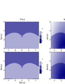
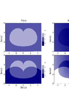
		Accelerating subsonic flow		Decelerating subsonic flow
		$c_{\text{sub1}}=1.8$, $c_{\text{sub2}}=1.9$.		$c_{\text{sub1}}=1.9$, $c_{\text{sub2}}=1.8$.
(a) (b)

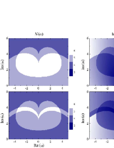
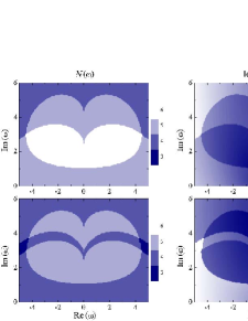
Figure 2: Stability analysis under outgoing boundary conditions for profiles with one discontinuity. Represented is the relevant portion of the upper-half complex frequency plane. From top to bottom and left to right: black hole and white hole configurations, accelerating and decelerating subsonic flows (the speed of sound $c$ is indicated for each region and the velocity $v$ is then obtained from the constrain $vc^{2}=1$; $c>1$ corresponds to a subsonic region, $c<1$ to a supersonic region; in addition, we use $\xi\,c=1$ in all our calculations). The lhs pictures represent the number $N$ of forbidden modes in the asymptotic regions. The rhs pictures represent the function $F(\omega)$ (to enhance the contrast, we have drawn the logarithm), and white points or regions, where $F(\omega)=0$, represent instabilities. In the upper pictures [case (a)], convergence has been imposed in both asymptotic regions. In the lower pictures [case (b)], convergence has been imposed only in the upstream asymptotic region. It is seen that black hole configurations are stable in both case (a) and (b), as are accelerating subsonic flows. White hole configurations are stable in case (a), but develop a huge continuous region of instabilities in case (b). Only a small strip of instabilities subsists in the decelerating subsonic flow, indicating that the major part of this unstable region is a genuine consequence of the existence of the white hole horizon. Note that continuous regions of instability correspond to $N<4$.

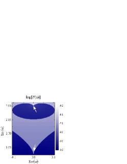
Figure 3: Two special zeros of the function $F(\omega)$ appear in the stability analysis of a black hole configuration (this plot is a zoom of the corresponding plot in Fig. 2). They are located at the boundary between regions with different number $N$ of prohibited modes. These points do not seem to represent real instabilities of the system (see appendix A).

IV.3 White hole configurations

Let us now consider flows decelerating from a supersonic regime (rhs) to a subsonic one (lhs). From the point of view of lhs observers, the geometric configuration possesses a white hole horizon. In GR, a white hole corresponds to the time reversal of a black hole. Therefore, unstable modes of a white hole configuration would correspond to stable (quasinormal) modes of the black hole. However, when modified dispersion relations are present, the precise definition of quasinormal modes cannot be based only upon the outgoing character of the modes, but their divergent or convergent character also has to be taken into account. Having in mind that in the acoustic approximation (proper Lorentzian behaviour) the outgoing character of a quasinormal mode implies that this mode diverges at the boundaries at infinity, it is reasonable to impose divergence as an additional defining requirement (apart from being outgoing) for a quasinormal mode in the presence of modified dispersion relations. Using this definition, we have checked (by analyzing the lower-half complex $\omega$ plane), that black hole configurations do not show any quasinormal (stable) eigenfrequency. Thus, we can conclude that one-dimensional white holes are stable. We emphasize here the word one-dimensional because we do not expect this situation to remain true in higher dimensions. We know for example that standard GR black holes in 3+1 dimensions possess quasinormal modes. We expect these quasinormal modes to subsist when taking into account departures from the acoustic (Lorentzian) dispersion relation; we only expect them to acquire modified eigenfrequencies. These quasinormal modes would then identify instabilities of the corresponding white hole configuration. We leave the analysis of the quasinormal modes in different analogue gravitational configurations in BECs for future work, since this analysis has its own subtleties.

The boundary conditions appropriate for the analysis of white hole-like configurations correspond to only having ingoing waves (due to time reversal) at the boundaries. But from the point of view of acoustic models in a laboratory, the analysis of the intrinsic stability of the flow (under the outgoing boundary conditions described above) is also interesting. This analysis also has particular relevance with regard to configurations with two horizons (see below).

In Fig. 2 we see that under outgoing boundary conditions the flow is stable when convergence is required in both asymptotic regions [case (a)], but exhibits a continuous region of instabilities at low frequencies when convergence is fulfilled only at the rhs [case (b)]. Indeed, in this continuous region $N=3$, in other words the algebraic system $\widetilde{\Lambda}_{ij}A_{ij}=0$ is underdetermined and any frequency is automatically an eigenfrequency.

When looking at the case of a completely subsonic flow suffering a deceleration (see Fig. 2), we find something similar. The system is clearly stable when convergence is imposed at the lhs, i.e. in case (a). Without convergence at the lhs, case (b), there is a continuous strip of instabilities which corresponds, as in the white hole case, to a region where $N=3$. However, this region is localized at relatively high frequencies and so disconnected from $\omega\sim 0$. We can say that part of the continuous region of instabilities found in the white hole configuration has its origin merely in the deceleration of the flow (giving rise to this high frequency strip). But there is still a complete region of instabilities that is genuine of the existence of a white hole horizon. In fact, by decreasing the healing length parameter $\xi$, the strip moves up to higher and higher frequencies, becoming less and less important as one approches the acoustic limit. However, the continuous region of instabilities associable with the horizon does not change its character in this process.

We can therefore conclude the following with regard to decelerating configurations. When convergence is fulfilled downstream, the configuration is stable, regardless of whether it contains a white hole horizon or not. When this convergence condition is dropped, there is a tendency to destabilization. In the presence of a white hole horizon, the configuration actually becomes dramatically unstable, since there is a huge continuous region of instabilities, and even perturbations with arbitrarily small frequencies destabilize the configuration. In the absence of such a horizon, only a small high-frequency part of this unstable region subsists.

IV.4 Black hole–white hole configurations

Consider flows passing from being subsonic to supersonic and then back to subsonic (Figure 4). The numerical algorithm we have followed to deal with this problem is equivalent to the one presented above, but with a larger set of equations. In this case we have $12$ arbitrary constants $A_{j}$, which have to satisfy $8+N$ equations: 4 matching conditions at each discontinuity and $N(0-8)$ additional conditions of the form $A_{j}=0$, corresponding to modes that do not fulfill the boundary conditions in a particular asymptotic region.

When convergence is imposed at the lhs, we do not find any instabilities, regardless of whether the fluid is globally accelerating or decelerating [the final lhs fluid velocity is larger or smaller than the initial rhs one respectively, see Figure 5 cases (a)]. Also when replacing the intermediate supersonic region by a subsonic one, thereby removing the acoustic horizons, the fluid is stable, independently of whether it is globally accelerating or decelerating.

When dropping the convergence condition at the lhs the situation changes completely. When the intermediate region is supersonic, i.e. in a black hole–white hole configuration, a discrete set of instabilities appears at low frequencies [Fig. 5 cases (b)]. It is worth mentioning that, when carefully looking at plots of type (a)-cases, we observe some traces of these zeros in the form of local minima which can be understood as particularly soft regions. These regions, although very close to zero in some situations, never give rise to real zeros, as we have carefully checked by zooming in. Notice that these local minima appear in regions with $N=5$ where a zero would mean a double degeneracy within the row vectors in the corresponding matrix $\tilde{\Lambda}_{ij}$. When the fluid is globally decelerating, additionally there is a continuous region of instabilities at higher frequencies. Indeed, in this region, as in the case of the white hole configuration, $N<4$, and so every frequency in this region automatically represents an instability. When the intermediate region is subsonic, the discrete set of local minima at low frequencies disappears, but the continuous strip of instabilities at higher frequencies persists in the case of a globally decelerating fluid. The discrete set of instabilities is therefore a genuine consequence of the existence of horizons.

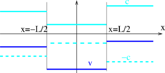
Figure 4: Flow and sound velocity profiles with step-like discontinuities simulating a black hole–white hole configuration.

The number of discrete zeros we find in the black hole–white hole configuration increases with the size $L$ of the supersonic region (see Fig. 6), while their $\text{Im}(\omega)$ decreases. This suggests that the region between the horizons acts as a sort of well discretizing some of the instabilities found for the white hole configurations. The larger the well, the larger the amount of instabilities, but the longer-lived these instabilities.

To summarize, when requiring convergence in both asymptotic regions, all the types of configurations with two discontinuities that we have discussed are stable. When not requiring convergence at the lhs, discretized instabilities appear associated with the presence of horizons.

		Black hole–white hole (globally accelerating)		Black hole–white hole (globally decelerating)
		$c_{\text{sub-lhs}}=1.8$, $c_{\text{super}}=0.7$, $c_{\text{sub-rhs}}=1.9$.		$c_{\text{sub-lhs}}=1.9$, $c_{\text{super}}=0.7$, $c_{\text{sub-rhs}}=1.8$.
(a) (b)
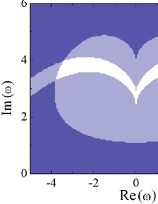
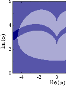
		Globally accelerating subsonic flow		Globally decelerating subsonic flow
		$c_{\text{sub-lhs}}=1.7$, $c_{\text{sub}}=1.8$, $c_{\text{sub-rhs}}=1.9$.		$c_{\text{sub-lhs}}=1.9$, $c_{\text{sub}}=1.8$, $c_{\text{sub-rhs}}=1.7$.
(a) (b)

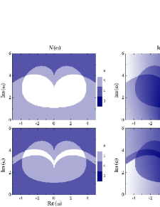
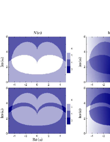
Figure 5: Stability analysis for profiles with two discontinuities. From top to bottom and left to right: globally accelerating and decelerating black hole–white hole configurations, globally accelerating and decelerating subsonic configurations. In all these plots we have used $L=2.5$ as the size of the intermediate region (see also caption under Fig. 2). When convergence is imposed in both asymptotic regions [case (a)], all the configurations are stable. When convergence is only imposed upstream [case (b)], the configurations with sonic horizons present a discrete set of instabilities at low frequencies, while the decelerating configurations show a small continuous unstable strip at high frequencies. The decelerating configuration with sonic horizons combines both types of instabilities.

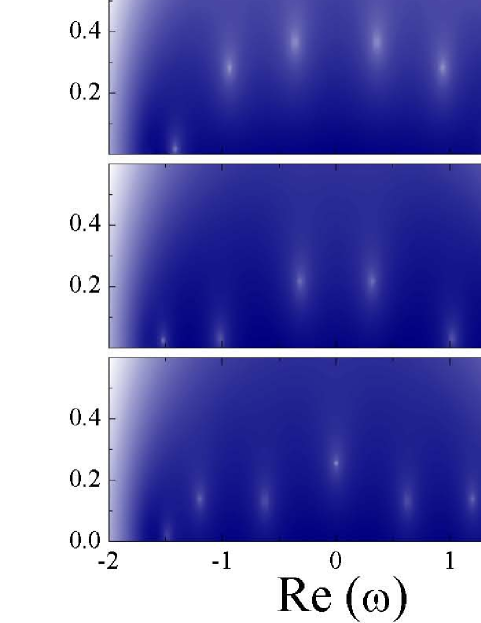
Figure 6: The number of discrete instabilities in the black hole–white hole configuration increases with the size $L$ of the intermediate supersonic region. In these plots we have used $c_{\rm sub-lhs}=1.8$, $c_{\rm super}=0.7$, $c_{\rm sub-rhs}=1.9$ (with their corresponding $v=1/c^{2}$) and $\xi\,c=1$.

IV.5 Black hole configurations with modified boundary conditions

We have seen in section IV.2 that configurations with a single black hole horizon do not possess instabilities in any situation. However, as we have just discussed, when they are continued into a white hole configuration, some instabilities can show up. Here, we would like to point out that the same happens if instead of extending the black hole configuration we introduce a wall (or sink) at a finite distance inside the supersonic region, described by other boundary conditions than the ones we have considered so far. For example, by replacing the lhs boundary conditions by $\theta|_{x=-L}=0$, we obtain Fig. 7. We can perfectly see how a set of discrete unstable modes appears.

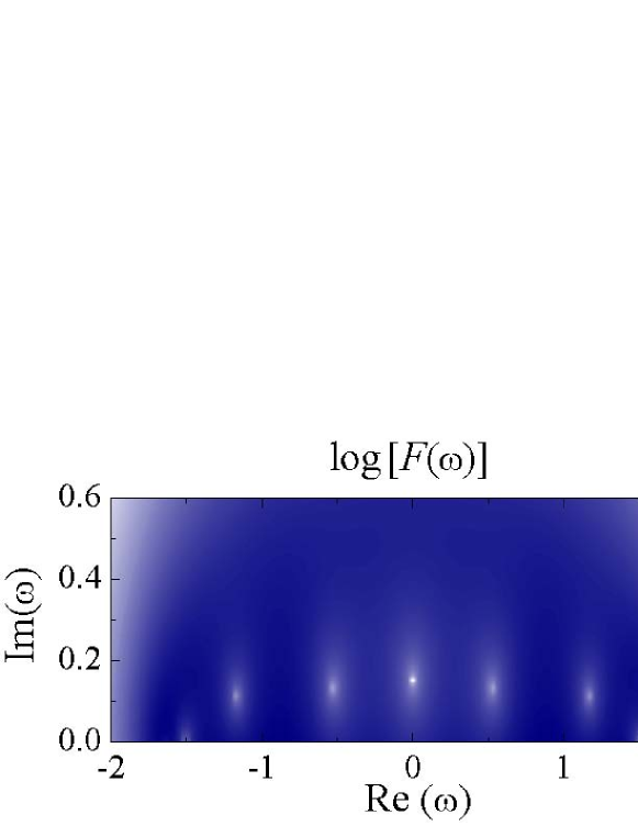
Figure 7: A discrete set of instabilities appears in a black hole configuration when the lhs asymptotic region representing the singularity is replaced by a wall or sink. In this plot we have used $c_{\rm sub}=1.9$ and $c_{\rm super}=0.7$ (with their corresponding $v=1/c^{2}$); in addition we have taken $L=6$ as the size of the, now finite, internal region.

V Discussion and conclusions

Let us start by discussing the stability of configurations with a single black hole-like horizon in analogue systems that incorporate superluminal dispersion relations. We have seen that by requiring purely outgoing and convergent boundary conditions in both asymptotic regions, these configurations do not show any signs of instability. The same applies when dropping the convergence condition downstream (i.e. on the lhs). This seems to contradict the results in Ref. sonicBH2 . There, the existence of a future (spacelike) singularity inside the black hole, from which no information is allowed to escape, was implemented by introducing a sink in the supersonic region at a finite distance from the horizon. Then, it was found that there were discrete instabilities in the system. However, these instabilities correspond to the following particular set of boundary conditions: i) At the asymptotic region, only convergent boundary conditions were imposed, without any condition about the direction of propagation (in- or outgoing) of the perturbations; ii) At the sink, two types of boundary conditions were required, specifically designed for dealing with symmetric and anti-symmetric configurations. In our language these boundary conditions correspond to $\{\theta^{\prime}|_{\rm sink}=0,n^{\prime}|_{\rm sink}=0\}$ and $\{\theta|_{\rm sink}=0,n|_{\rm sink}=0\}$ respectively. In comparing this result with ours we have checked two important facts. On the one hand, their unstable modes have ingoing contributions at the asymptotic region. On the other hand, the boundary conditions at the sink are such that they combine outgoing and ingoing contributions – their sink implementation makes waves reaching the sink bounce back towards the horizon. These two facts are responsible for the unstable behaviour of these black hole-like configurations. If no energy is introduced into the system from the asymptotic region (in other words, if only outgoing perturbations are allowed) and moreover any bouncing at the sink is eliminated, then these configurations are stable. This is in agreement with the result found in Ref. leonhardt .

In the case of configurations with a single white hole horizon, we have seen that with outgoing and convergent boundary conditions in both asymptotic regions, there are no instabilities in the system. However, when eliminating the convergence condition in the downstream asymptotic region, one finds a continuous region of instabilities surrounding $\omega=0$. Thus, we see that these white hole configurations are stable only when the boundary conditions are sufficiently restrictive.

When analyzing configurations connecting two different subsonic regions, we have also seen that, again, when convergence is required at the lhs, they are stable. But when this convergence condition is relaxed, globally decelerating configurations tend to become unstable, whereas globally accelerating ones remain stable. The instabilities of these decelerating configurations without horizons (i.e. purely subsonic ones) show up, however, in a small strip at high frequencies. In contrast, white hole configurations present instabilities for a wide range of frequencies, starting from arbitrarily small values. This points out that the presence of a white hole horizon drastically stimulates the instability of the configuration.

With regard to the black hole–white hole configurations, we have seen that, as before, with outgoing and convergent boundary conditions, they are stable. However, when relaxing the convergence condition downstream, they develop a discrete set of unstable modes.

In the analysis of the black hole laser instability in Ref. jacobson , the authors found that these black hole–white hole configurations were intrinsically unstable. However, they did not analyze what happens to the modes at the lhs infinity. Our analysis shows that by restricting the possible behaviour of the modes in the downstream asymptotic region, one can eliminate the unstable behaviour of the black hole laser. This is in agreement with the results in Refs. sonicBH1 ; sonicBH2 . There, the instabilities can in some cases be removed by requiring periodicity, that is, by imposing additional boundary conditions to the modes.

To sum up, we have shown the high sensibility of the stability not only on the type of configuration (the presence of a single horizon or of two horizons, the accelerating or decelerating character of the fluid), but particularly on the boundary conditions. With outgoing boundary conditions, when requiring convergence at the downstream asymptotic region, both black hole and white hole configurations are stable (and also the combination of both into a black hole–white hole configuration). When relaxing this convergence condition at the lhs, configurations with a single black hole horizon remain stable, whereas white hole and black hole–white hole configurations develop instabilities not present in (subsonic) flows without horizons.

Appendix A Zeros at the boundaries of the regions in $N(\omega)$

Given an $\omega$, one can find its four associated $k$ roots, $\{k_{j}\}$. If instead of $\omega$ one takes $\tilde{\omega}=-\omega^{*}$, it can be seen that the new roots $\{\tilde{k}_{j}\}$ are just $\{-k_{j}^{*}\}$. For this reason the function $F(\omega)$ is mirror symmetric with respect to the imaginary axis (this is seen in all our figures). Now, when $\omega$ is pure imaginary ($\omega=-\omega^{*}$), the set $\{k_{j}\}$ has to be equal to the set $\{-k_{j}^{*}\}$. There are three posibilities. Either all four roots are pure imaginary, two are imaginary and the other two complex satisfying $k_{j}=-k_{l}^{*}$, with $j\neq l$, or there are two pairs of complex roots satisfying $k_{j}=-k_{l}^{*}$. When moving through the imaginary $\omega$ axis, there are points at which there is a transition from one of these possibilities to another. At any transition point there has to be a pair of imaginary roots with equal value. Defining $\omega^{\prime\prime}\equiv{\rm Im}(\omega)$ and $\kappa\equiv-ik$, the dispersion equation (8) can be written as

$$(\omega^{\prime\prime}-v\kappa)^{2}-\left(c^{2}-{1\over 4}c^{2}\xi^{2}\kappa^{2}\right)\kappa^{2}=0.$$ (19)

This is a fourth order polynomial in $\kappa$ with real coefficients. If this polynomial has two equal real roots then we know that the derivative with respect to $\kappa$ of the polynomial has to be zero at that point. It is not difficult to see that this also implies that the derivative with respect to $\kappa$ of the function

$$(w-v\kappa)\mp\left(c^{2}-{1\over 4}c^{2}\xi^{2}\kappa^{2}\right)^{1/2}\kappa$$ (20)

has to be zero at this same point. But this derivative coincides with the definition of the group velocity given in (18) (when $\omega$ and $k$ are pure imaginary, $d\omega/dk$ is directly real). Therefore, we conclude that at any transition point on the imaginary $\omega$-axis we have degeneracy: at least two imaginary $k$ roots with equal value. At the same time, the group velocity associated with them becomes zero. This is why these points are located at the boundary between regions with a different number of forbidden modes: these are places in which outgoing modes transform into ingoing ones. The zero that appears in the function $F(\omega)$ at these points is due to the degeneracy and does not tell us anything about the existence or not of a real instability there. To know whether a real instability appears, one first has to find the actual four independent solutions of equations (12) at the point that led to the degeneracy. Let us check under which circumstances one can find a solution of the form

$$\widetilde{n}_{1}(x,t) =A_{1}\,x\,e^{i(kx-\omega)t},$$ (21a)

$$\theta_{1}(x,t) =B_{1}\,x\,e^{i(kx-\omega)t}+B_{2}e^{i(kx-\omega)t}.$$ (21b)

For these expressions to be a solution of Eqs. (12), the following conditions have to be satisfied:

$$\begin{pmatrix}i(\omega-vk)&&c^{2}k^{2}\\ \\ 1+{1\over 4}\xi^{2}k^{2}&&-i(\omega-vk)\end{pmatrix}\begin{pmatrix}A_{1}\\ \\ B_{1}\end{pmatrix}=0,$$ (22)

$$\begin{pmatrix}i(\omega-vk)&&c^{2}k^{2}\\ \\ 1+{1\over 4}\xi^{2}k^{2}&&-i(\omega-vk)\end{pmatrix}\begin{pmatrix}0\\ \\ B_{2}\end{pmatrix}+\begin{pmatrix}-v&&-2ic^{2}k\\ \\ -{1\over 2}i\xi^{2}k&&v\end{pmatrix}\begin{pmatrix}A_{1}\\ \\ B_{1}\end{pmatrix}=0.$$ (23)

From the first condition we obtain that the dispersion relation (8) has to be fulfilled. As a consequence we also find that $B_{1}=A_{1}(\omega-vk)/(ic^{2}k^{2})$. Now, from the second condition we obtain

$$\begin{pmatrix}-c^{2}k^{2}\\ \\ i(\omega-vk)\end{pmatrix}={A_{1}\over B_{2}}\begin{pmatrix}-v&&-2ic^{2}k\\ \\ -{1\over 2}i\xi^{2}k&&v\end{pmatrix}\begin{pmatrix}1\\ \\ {(\omega-vk)\over ic^{2}k^{2}}\end{pmatrix}$$ (24)

This is a system of two equations from which, eliminating $A_{1}/B_{2}$ and after some rearranging, we obtain:

$$c^{2}k+{1\over 2}c^{2}\xi^{2}k^{3}+v(\omega-vk)=0.$$ (25)

This is exactly the condition for a vanishing group velocity (18). Therefore, when functions in the form of plane waves do not lead to four linearly independent solutions, but for example two are “degenerate”, then we can use the previous solution (21) avoiding this degeneracy. Once we have the actual four independent solutions of the problem, they have to be matched with the four solutions in the other region (typically these will have the form of plane waves, unless we are in a very special situation in which degeneracy occurs in both regions at the same time) and see whether there is a combination satisfying all the boundary conditions.

Although we haven’t made such a full detailed calculation, the fact that this kind of situation occurs in any type of flow indicates that it is safe to assume that they do not represent real instabilities, as already mentioned.

Appendix B Bogoliubov representation

All calculations and numerical simulations presented in the text have been performed independently by using the acoustic representation and the Bogoliubov representation sonicBH1 ; sonicBH2 described in this appendix. We have found identical results with the two methods, double checking in this way the absence of numerical artifacts.

Consider a one-dimensional setup with a potential $V_{\rm ext}$ that produces a profile for the speed of sound of the form

$$c(x)=\left\{\begin{array}[]{ll}c_{0},&x<0\\ c_{0}[1+(\sigma-1)x/\epsilon],&0<x<\epsilon\\ \sigma c_{0},&\epsilon<x\end{array}\right..$$ (26)

We will assume $\sigma>1$ and a flow velocity in the inward ($x\to-\infty$) direction, i.e. a black hole-like configuration for a rhs observer. The limit $\epsilon\rightarrow 0$ provides the same profile we have discussed in the main text.

The condensate wave function can be written as the sum of a stationary background state $\psi_{0}$ and a perturbation $\phi$ satisfying

$$i\partial_{t}\phi=-\partial_{x}^{2}\phi/2+(c^{2}-v^{2}/2+\partial_{x}^{2}c/2c)\phi+c^{2}e^{2i\int^{x}v}\phi^{*},$$ (27)

that will then be expanded into Bogoliubov modes

$$\phi=u_{\omega}(x)e^{-i\omega t}+w^{*}_{\omega}(x)e^{i\omega^{*}t}.$$ (28)

¿From now on, we drop the subindex $\omega$, but remember that all equations should be valid for every (complex) frequency $\omega$ separately.

The assumption of a small $\epsilon$ leads to a linear solution for the modes $u$ and $w$ in the intermediate region $0<x<\epsilon$. Together with the transition conditions at $x=0$ and $x=\epsilon$, which substitute the singular character of $\partial_{x}^{2}c/c$ at those points, this leads to the following connection formulas (in the limit $\epsilon\rightarrow 0$), see Ref. sonicBH2 :

$$[u/c]= 0, [\partial_{x}(cu)]= 0,$$ (29)

$$[w/c]= 0, [\partial_{x}(cw)]= 0,$$ (30)

where as before we have used the notation $[u]=u|_{x\to 0^{+}}-u|_{x\to 0^{-}}$.

Let us write the density and phase in terms of the stationary values plus perturbations:

$$n=n_{0}+\text{\sl g}^{-1}\widetilde{n}_{1},\qquad\theta=\theta_{0}+\theta_{1},$$ (31)

and note that the matching condition for the background velocity potential is $[\theta_{0}]=0.$

The relation between the acoustic and the Bogoliubov representation of the perturbations can easily be obtained by noting that, to first order,

$$\phi=\sqrt{m/\text{\sl g}}\,c(\widetilde{n}_{1}/2mc^{2}+i\theta_{1})e^{i\theta_{0}},$$ (32)

where we have used the fact that $c^{2}=\text{\sl g}n_{0}/m$. Note that $\widetilde{n}_{1}$ and $\theta_{1}$ are real. Then, comparison of Eq. (32) with the Bogoliubov mode expansion $\phi=ue^{-i\omega t}+w^{*}e^{i\omega^{*}t}$ yields

$$u =\sqrt{m/\text{\sl g}}\,c(\widetilde{n}_{1}/2mc^{2}+i\theta_{1})e^{i\theta_{0}},$$ (33)

$$w =\sqrt{m/\text{\sl g}}\,c(\widetilde{n}_{1}/2mc^{2}-i\theta_{1})e^{-i\theta_{0}}.$$ (34)

We then have

$$[u/c]\propto[(\widetilde{n}_{1}/2c^{2}+i\theta_{1})e^{i\theta_{0}}]\propto[\widetilde{n}_{1}/2c^{2}+i\theta_{1}]$$ (35)

and likewise for $w$. Comparing with Eq. (29), we obtain

$$[\widetilde{n}_{1}/c^{2}]\propto[u/c]+[w/c]=0,$$ (36)

$$[\theta_{1}]\propto[u/c]-[w/c]=0,$$ (37)

which correspond to two of the conditions in Eqs. (15).

Taking into account that $[\theta_{0}]=[c^{2}v]=[\theta_{1}]=0$ and that $\partial_{x}c_{L}=\partial_{x}c_{R}=0$, we can write

$$[\partial_{x}(cu)]\propto \;i[v\widetilde{n}_{1}]/2+[\partial_{x}\widetilde{n}_{1}]/2+i[c^{2}\partial_{x}\theta_{1}],$$ (38)

$$[\partial_{x}(cw)]\propto -i[v\widetilde{n}_{1}]/2+[\partial_{x}\widetilde{n}_{1}]/2-i[c^{2}\partial_{x}\theta_{1}].$$ (39)

In other words $[\partial_{x}\widetilde{n}_{1}]=0$ and $[v\widetilde{n}_{1}/2+c^{2}\partial_{x}\theta_{1}]=0$. Because of the continuity equation $vc^{2}=\text{const}$, we have $[v\widetilde{n}_{1}]\propto[n_{1}/c^{2}]=0$, so that the boundary conditions ultimately become

$$[\partial_{x}\widetilde{n}_{1}] =0, [c^{2}\partial_{x}\theta_{1}] =0,$$ (40)

i.e. the other two conditions in Eqs. (15) with the corresponding simplifications.

References

- (1) A. Ashtekar and J. Lewandowski, “Background independent quantum gravity: A status report,” Class. Quant. Grav. 21, R53 (2004) [arXiv:gr-qc/0404018].
- (2) C. Barceló, S. Liberati and M. Visser, “Analogue Gravity,” Living Rev. Relativity 8, (2005), 12. URL (cited on 02-20-06): http://www.livingreviews.org/lrr-2005-12 [arXiv:gr-qc/0505065].
- (3) M. Novello, M. Visser and G. Volovik (eds.), Artificial black holes, World Scientific, Singapore (2002).
- (4) C. Barceló, S. Liberati and M. Visser, “Analog gravity from Bose-Einstein condensates,” Class. Quant. Grav. 18, 1137 (2001) [arXiv:gr-qc/0011026].
- (5) F. Dalfovo, S. Giorgini, L. Pitaevskii and S. Stringari, “Theory of Bose-Einstein condensation in trapped gases , Rev. Mod. Phys. 71, 463 (1999) [arXiv:cond-mat/9806038].
- (6) Y. Castin, “Bose-Einstein condensates in atomic gases: simple theoretical results,” in: Coherent atomic matter waves, Lecture Notes of Les Houches Summer School, edited by R. Kaiser, C. Westbrook, and F. David, EDP Sciences and Springer-Verlag (2001).
- (7) W. Ketterle, D.S. Durfee and D.M. Stamper-Kurn, “Making, probing and understanding Bose-Einstein condensates , in: Bose-Einstein condensation in atomic gases, Proceedings of the International School of Physics ‘Enrico Fermi’, edited by M. Inguscio, S. Stringari and C.E. Wieman, IOS Press, Amsterdam (1999) [arXiv:cond-mat/9904034].
- (8) L. J. Garay, J. R. Anglin, J. I. Cirac and P. Zoller, “Black holes in Bose-Einstein condensates,” Phys. Rev. Lett. 85, 4643 (1999) [arXiv:gr-qc/0002015].
- (9) L. J. Garay, J. R. Anglin, J. I. Cirac and P. Zoller, “Sonic black holes in dilute Bose-Einstein condensates,” Phys. Rev. A 63, 023611 (2001) [arXiv:gr-qc/0005131].
- (10) T. Padmanabhan, “Event horizon: Magnifying glass for Planck length physics,” Phys. Rev. D 59, 124012 (1999) [arXiv:hep-th/9801138].
- (11) U. Leonhardt, T. Kiss, and P. Ohberg, “Theory of elementary excitations in unstable Bose-Einstein condensates and the instability of sonic horizons,” Phys. Rev. A 67, 033602 (2003).
- (12) S. Corley and T. Jacobson, “Black hole lasers,” Phys. Rev. D 59, 124011 (1999) [arXiv:hep-th/9806203].
- (13) K. D. Kokkotas and B. G. Schmidt, “Quasi-normal modes of stars and black holes,” Living Rev. Rel. 2, 2 (1999) [arXiv:gr-qc/9909058].
- (14) W. G. Unruh, “Experimental Black Hole Evaporation,” Phys. Rev. Lett. 46, 1351 (1981).
- (15) M. Visser, “Acoustic black holes: Horizons, ergospheres, and Hawking radiation,” Class. Quant. Grav. 15, 1767 (1998) [arXiv:gr-qc/9712010].