Counting of Black Hole Microstates

Abstract

The entropy of a black hole can be obtained by counting states in loop quantum gravity. The dominant term depends on the Immirzi parameter involved in the quantization and is proportional to the area of the horizon, while there is a logarithmic correction with coefficient -1/2.

It is an honour and a pleasure to write in the volume dedicated to Professor Amal Kumar Raychaudhuri, eminent theoretical physicist and revered teacher of generations of Physics students. The theory of gravitation, with which he preoccupied himself, is progressing steadily, and although a full quantum theory is not yet at hand, a lot of interesting results are available.

A framework for the description of quantum gravity using holonomy variables has become popular as loop quantum gravity ash . A start was made in this work in the direction of counting of black hole microstates. Further progress was made in gm0 , meissner and in gm . In the present article we shall try to tie up some loose ends left there. Other discussions of the subject can be found in tamaki ; 0511084 .

In this approach, there is a classical isolated horizon and quantum states are sought to be built up by associating spin variables with punctures on the horizon. The entropy is obtained by counting the possible states that are consistent with a particular area, or more precisely with a particular eigenvalue of the area operator ash .

We set units such that $4\pi\gamma\ell_{P}^{2}=1$, where $\gamma$ is the Immirzi parameter and $\ell_{P}$ the Planck length. Equating the classical area $A$ of the horizon to the eigenvalue of the area operator we find

$$A=2\sum_{p=1}^{N}\sqrt{j_{p}(j_{p}+1)}\;,$$ (1)

where the $p$-th puncture carries a spin $j_{p}$, more accurately an irreducible representation labelled by $j_{p}$, and contributes a quantum of area $2\sqrt{j_{p}(j_{p}+1)}$ to the total area spectrum. For mathematical convenience let us replace the half-odd integer spins by integers $n_{p}=2j_{p}$, which makes the area equation $A=\sum_{p}\sqrt{n_{p}(n_{p}+2)}$. Henceforth, $n_{p}$ will be referred to as the ‘spin’ carried by the $p$-th puncture. A puncture carrying zero spin contributes nothing to the spectrum, hence such punctures are irrelevant. Since the minimum ‘spin’ each puncture should carry is unity the total number of punctures cannot exceed $A/\sqrt{3}$. At the same time, the largest ‘spin’ a puncture can carry is also bounded, $n\leq N$, where $\sqrt{N(N+2)}=A$.

A sequence of ‘spins’ $n_{p}$, each $1\leq n_{p}\leq N$, will be called permissible if it obeys (1). The $p$-th puncture gives $(n_{p}+1)$ number of quantum states. In this way each permissible sequence gives rise to a certain number of quantum states. The task is to find the total number of states for all permissible sequences. Let it be $d(A)$. One can subdivide the problem as follows: Fix any puncture, say $p=1$. Consider the subset of all permissible sequences such that puncture 1 carries ‘spin’ 1. For such sequences the area equation (1) reads

$$\sum_{p\neq 1}\sqrt{n_{p}(n_{p}+2)}=A-\sqrt{3}\;.$$ (2)

So the total number of quantum states given by all sequences obeying (2) is $d(A-\sqrt{3})$. But the puncture 1 itself gives two states. Therefore, the total number quantum states given by the subset of permissible sequences in which puncture 1 carries ‘spin’ 1 is $2d(A-\sqrt{3})$. In the next step consider the subset of all permissible sequences such that puncture 1 carries ‘spin’ 2. Arguments similar to the above leads to the total number of states for such subset of sequences as $3d(A-2\sqrt{2})$. Continuing this process we end up with a recurrence relation

$$d(A)=\sum_{n=1}^{N-1}(n+1)d(A-\sqrt{n(n+2)})+N+1.$$ (3)

This is similar to the relation in meissner , but differs from it in having all values of $m=-j,-j+1,...+j$ allowed.

In solving (3) we employ a trial solution $d(A)=\exp(\lambda A)$. Then (3) puts a condition on $\lambda$:

$$\sum_{n=1}^{N}(n+1)\,e^{-\lambda\sqrt{n(n+2)}}=1\;.$$ (4)

Therefore, a solution for $\lambda$ obeying the above equation implies a solution of the recurrence relation (3). For large area $A\gg 1$, we have $N\gg 1$. Moreover, for $\lambda=o(1)$ the summand falls off exponentially for large $n$. So formally we can extend the sum up to infinity. This numerically yields $\lambda\simeq 0.861$. The error we make in estimating $\lambda$ by extending the sum all the way to infinity is $o(e^{-A})$. The total degeneracy $d(A)$ then gives rise to a Boltzmann entropy $S(A)=\ln d(A)=\lambda A$. In physical units

$$S(A)={\lambda A\over 4\pi\gamma\ell_{P}^{2}}\;,$$ (5)

which yields $A/4\ell_{P}^{2}$ if we choose the parameter $\gamma=\lambda/\pi$. This is the basic idea behind the counting and thereby, making a prediction for the $\gamma$-parameter in order that an entirely quantum geometric calculation matches a semi-classical formula. Thus we cannot derive the semiclassical world but can adjust our parameters in the theory such that the semiclassical world emerges.

In the above counting process we completely miss which configuration of spins dominates the counting, in other words contributes the largest number of quantum states. A common misconception is that the smallest ‘spin’ $n=1$ at every puncture gives rise to the largest number of quantum states. It arises from the intuition that such configuration maximizes the number of punctures and is therefore semiclassically favoured. The following analysis will show that such an intuition is incorrect. We focus on punctures carrying identical spins. This is somewhat in analogy with statistical mechanics where we look for particles carrying the same energy. Let the number of punctures carrying ‘spin’ $n$ be $s_{n}$. So in the area equation (1) the sum over punctures can be replaced by the sum over spins

$$A=\sum_{n}s_{n}\sqrt{n(n+2)}\;.$$ (6)

Equation (6) further symbolizes the fact that spins are more fundamental in this problem than punctures. A configuration of ‘spins’ $s_{n}$ will be called permissible if it obeys (6). Each configuration yields $\prod_{n}(n+1)^{s_{n}}$ quantum states but each of the configurations can be chosen in $(\sum s_{n})!/\prod s_{n}!$ ways (punctures are considered distinguishable). Therefore, the total number of quantum states given by such a configuration is

$$d_{s_{n}}={(\sum_{n}s_{n})!\over\prod_{n}s_{n}!}\prod_{n}(n+1)^{s_{n}}\;.$$ (7)

However, the configuration in (7) may not be permissible. To obtain a permissible configuration we maximize $\ln d_{s_{n}}$ by varying $s_{n}$ subject to the constraint (6). In the variation we assume that $s_{n}\gg 1$ for each $n$ (or only such configurations dominate the counting). Such an assumption clearly breaks down if $A\sim o(1)$. The variational equation $\delta\ln d_{s_{n}}=\lambda\delta A$, where $\lambda$ is a Lagrange multiplier, gives

$${s_{n}\over\sum s_{n}}=(n+1)\,e^{-\lambda\sqrt{n(n+2)}}\;.$$ (8)

Clearly, for consistency, $\lambda$ obeys (4) with $N=\infty$ (cf. krasnov ). As already observed this hardly makes a difference, more precisely the differences are exponentially suppressed $o(e^{-A})$ for large areas. Moreover, although each $s_{n}\gg 1$, the sum $\sum s_{n}$ is convergent, since large $n$ terms are exponentially suppressed. This can be explicitly seen by plugging in (8) into (6), which yields

$$\sum s_{n}=A\left[\sum(n+1)\sqrt{n(n+2)}\,e^{-\lambda\sqrt{n(n+2)}}\right]^{-1}=0.342A\;.$$ (9)

Plotting (8) we find how the configuration contributing the largest number of quantum states is distributed over all spins. The maximum number of punctures carry integer 1 (which are truly spin 1/2), as the intuition suggests, but surprisingly all other spins also contribute.

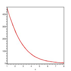
Figure 1: Dominant configuration.

Let us denote the configuration (8) dominating the counting by $\bar{s}_{n}$. The total number of quantum states is obviously $d=\sum_{s_{n}}d_{s_{n}}$ where the sum extends over all permissible configurations. However, the largest number of states come from some dominant configuration $\bar{s}_{n}$. So we can expand $d$, more accurately the entropy $\ln d$, around this dominant configuration and the result should be expressible in the form $\ln d=\ln d_{\bar{s}_{n}}-{\textstyle{1\over 2}}\sum_{n,n^{\prime}}\delta s_{n}K_{nn^{\prime}}\delta s_{n^{\prime}}+o(\delta s_{n}^{2})$, where $\delta s_{n}$ satisfies the area equation $\sum\delta s_{n}\sqrt{n(n+2)}=0$, which follows by requiring that the displaced configuration $\bar{s}_{n}+\delta s_{n}$ also obeys the area equation (6). One may wonder at this point whether such a condition can ever be met since $\delta s_{n}$ are integers whereas $\sqrt{n(n+2)}$ are irrational. Strictly speaking in the area equation (6) we require that the sum $\sum s_{n}\sqrt{n(n+2)}$ should be close to $A$. In other words a range $-\Delta\leq A\leq\Delta$, where $\Delta\ll A$, must exist such that the sum lies in the range. This amounts to saying that $\sum\delta s_{n}\sqrt{n(n+2)}$ be a number $\epsilon\sim o(1)$, where $\epsilon$ may vary with configurations but the variation is slow. The matrix $K_{nn^{\prime}}$ which depends on $\bar{s}_{n}$ is symmetric. A simple calculation gives $K_{nn^{\prime}}=\delta_{nn^{\prime}}/\bar{s}_{n}-1/(\sum\bar{s}_{m})$. The total number of states can be expressed as

$$d=d_{\bar{s}_{n}}\sum_{-\infty}^{\infty}e^{-{\textstyle{1\over 2}}\sum_{n,n^{\prime}}\delta s_{n}K_{nn^{\prime}}\delta s_{n^{\prime}}}\delta(\sum\delta s_{n}\sqrt{n(n+2)})$$ (10)

where the sum extends over all fluctuations. The large fluctuations die out exponentially. The Gaussian sum over fluctuations would have produced a factor $1/\sqrt{{\rm det}(K)}$ if the delta function were not there. It is easy to see that $K$ has a zero eigenvalue ($\sum K_{nn^{\prime}}\bar{s}_{n^{\prime}}=0$), so this hypothetical factor would be divergent. But the delta function makes the sum over the zero mode of $K$ finite. Note that each nonzero eigenvalue of $K$ scales like $1/A$, so the fluctuations $\delta s_{n}$, which have to be rewritten in terms of normal modes $\delta s_{n}^{\prime}$ of $K$, have to be converted to $\delta s_{n}^{\prime}/\sqrt{A}$, producing extra factors of $\sqrt{A}$ for each summation. As one summation is removed by the delta function,

$$d=Cd_{\bar{s}_{n}}\Big{[}\prod_{n}\sqrt{A}\,\Big{]}/\sqrt{A},$$ (11)

where $C$ does not involve $A$. Plugging (8) into (7) and neglecting $o(1)$ factors we find

$$d_{\bar{s}_{n}}=\exp(\lambda A)[\sum\bar{s}_{n}]^{1/2}/\prod_{n}(2\pi\,\bar{s}_{n})^{1/2}.$$ (12)

Noting that the factors of $\sqrt{A}$ cancel, we get $d=\exp(\lambda A)$ up to factors of $o(1)$ which will anyway be of $o(1)$ in the entropy and therefore have been neglected throughout in the calculation.

The above steps illustrate the basic points of the calculation which now can be adapted to the actual counting. The actual counting problem involves another crucial condition: Each puncture carrying a representation labelled by ‘spin’ $n$ must be associated with a state $|n,m\rangle$ where $m$ is half-odd integer valued spin projections, $-n/2\leq m\leq n/2$. The condition is that $\sum_{p}m_{p}=0$ where the sum extends over all punctures. Therefore, a sequence of ‘spins’ $n_{p}$ is permissible if it obeys the area equation and the spin projection equations simultaneously. The task is to count the number of states for all such permissible sequences. A recurrence relation, similar to (3), can be found also in this case. Following meissner we relax the spin-projection equation to $\sum_{p}m_{p}=\nu$ where $\nu$ is a half-odd integer that can take any sign. Let the total number of states be $d_{\nu}(A)$. As before fix a puncture, say 1, and let it carry ‘spin’ 1. For such sequences the area and the spin projection equations become $\sum_{p\neq 1}\sqrt{n_{p}(n_{p}+2)}=A-\sqrt{3}$ and $\sum_{p}m_{p}=\nu\pm 1/2$ respectively. Therefore, the number of quantum states for all permissible configurations such that the puncture 1 carries ‘spin’ 1 is $d_{\nu+1/2}(A-\sqrt{3})+d_{\nu-1/2}(A-\sqrt{3})$. Continuing this process as before we end up with the recurrence relation

$$d_{\nu}(A)=\sum_{n=1}^{N-1}\sum_{m=-n/2}^{n/2}d_{\nu-m}(A-\sqrt{n(n+2)})+1,$$ (13)

where the largest ‘spin’ $N$ contributes only one state to the above sum, provided $\nu$ belongs to the set of allowed values of $m=\{-N/2,...N/2\}$. In order to solve (13) we consider the Fourier transform of $d_{\nu}(A)$

$$d_{\nu}(A)=\int_{-2\pi}^{2\pi}{d\omega\over 4\pi}\;d_{\omega}(A)\,e^{i\omega\nu}$$ (14)

and re-express the recurrence relation in terms of $d_{\omega}(A)$:

$$d_{\omega}(A)=\sum_{n}d_{\omega}(A-\sqrt{n(n+2)})\sum_{m}\cos(m\omega)\;.$$ (15)

In an attempt to solve (15) we again employ a trial solution $d_{\omega}(A)=\exp(\lambda_{\omega}A)$, which on being plugged into the recurrence relation yields a condition on $\lambda_{\omega}$:

$$1=\sum_{n}e^{-\lambda_{\omega}\sqrt{n(n+2)}}\sum_{m}\cos(m\omega)\;.$$ (16)

The above equation (16) clearly shows that $\lambda_{\omega}$ is a periodic function of $\omega$. It is also multi-valued. However, it has a local maximum at $\omega=0$ and in a small neighbourhood of this maximum it can be approximated by a power series $\lambda_{\omega}=\lambda+a_{2}\omega^{2}+a_{4}\omega^{4}+\cdots$. Values of $\lambda,a_{2},a_{4},...$ etc can then be obtained from (16) by comparing various powers of $\omega$. It can be easily shown that $\lambda$ obeys the same recurrence relation as (3), therefore the same as before,

$$a_{2}=-{\sum e^{-\lambda\sqrt{n(n+2)}}\sum{1\over 2}m^{2}\over\sum(n+1)\sqrt{n(n+2)}e^{-\lambda\sqrt{n(n+2)}}}\simeq-0.151\;.$$ (17)

Finally, we are interested in

$$d_{0}(A)=\int_{-2\pi}^{2\pi}{d\omega\over 4\pi}\;e^{\lambda_{\omega}A}={\alpha\over\sqrt{A}}\;e^{\lambda A}\;,\quad{\rm where}\;\alpha\sim o(1)\;,$$ (18)

which yields an entropy $S(A)=\lambda A-{1\over 2}\ln A$, or

$$S(A)={\lambda A\over 4\pi\gamma\ell_{P}^{2}}-{1\over 2}\ln A$$ (19)

in physical units. Thus, incorporation of the projection equation $\sum m=0$ does not alter the leading expression of entropy, hence does not give a different requirement on the $\gamma$-parameter to make the leading entropy agree with the semiclassical formula, but gives a universal log-correction to the semiclassical formula with a factor of $1/2$.

The counting using the dominant configuration is cleaner when the projection equation is incorporated. Here we present the detailed calculation. As before, let $s_{n,m}$ denotes the number of punctures carrying ‘spin’ $n$ and projection $m$. The area and spin projection equations take the form

$$A=\sum_{n,m}s_{n,m}\sqrt{n(n+2)}\;,\quad 0=\sum_{n,m}ms_{n,m}\;.$$ (20)

A configuration $s_{n,m}$ will be called permissible if it satisfies both of these equations (20). Since now the $m$-quantum numbers are also specified each puncture is in a definite quantum state specified by two quantum numbers $n,m$. The total number of quantum states for all configurations is the number of ways a configuration can be chosen. This can be done in two steps. Note that $\sum_{m}s_{n,m}=s_{n}$. So first, the configuration $s_{n}$ can be chosen in $(\sum s_{n})!/\prod s_{n}!$ ways. Then out of $s_{n}$ the configuration $s_{n,m}$ can be chosen in $s_{n}!/\prod_{m}s_{n,m}!$ ways and finally a $\prod_{n}$ has to be taken. Thus we get

$$d_{s_{n,m}}={(\sum_{n}s_{n})!\over\prod_{n}s_{n}!}\prod_{n}{s_{n}!\over\prod_{m}s_{n,m}!}={(\sum_{n,m}s_{n,m})!\over\prod_{n,m}s_{n,m}!}\;.$$ (21)

To obtain permissible configurations which contribute the largest number of quantum states we maximize $\ln d_{s_{n,m}}$ by varying $s_{n,m}$ subject to the two conditions (20). The calculation is identical as before and the result can be expressed in terms of two Lagrange multipliers $\lambda,\alpha$

$${s_{n,m}\over\sum s_{n,m}}=e^{-\lambda\sqrt{n(n+2)}-\alpha m}\;.$$ (22)

Consistency requires that $\lambda$ and $\alpha$ be related to each other as $\sum_{n}e^{-\lambda\sqrt{n(n+2)}}\sum_{m}e^{-\alpha m}=1$. In order that (22) satisfy the spin projection equation we must require the sum $\sum_{n}e^{-\lambda\sqrt{n(n+2)}}\sum_{m}me^{-\alpha m}=0$. This is possible if and only if $\sum_{m}me^{-\alpha m}=0$ for all $n$, which essentially implies $\alpha=0$. (The value $2i\pi$ is excluded by positivity requirements.) Therefore, the condition on $\lambda$ becomes the same as before. The sum $\sum s_{n,m}=\sum s_{n}$ is also the same as before.

The total number of quantum states for all permissible configurations is clearly $d(A)=\sum_{s_{n,m}}d_{s_{n,m}}$. To estimate $d(A)$ we again expand $\ln d$ around the dominant configuration (22), denoted by $\bar{s}_{n,m}$. As before, it gives $\ln d=\ln d_{\bar{s}_{n,m}}-{1\over 2}\sum\delta s_{n,m}K_{n,m;n^{\prime}m^{\prime}}\delta s_{n^{\prime}m^{\prime}}+o(\delta s_{n,m}^{2})$ where $K$ is the symmetric matrix $K_{n,m;n^{\prime}m^{\prime}}=\delta_{nn^{\prime}}\delta_{mm^{\prime}}/\bar{s}_{n,m}-1/\sum_{k,l}\bar{s}_{k,l}$. All variations $\bar{s}_{n,m}+\delta s_{n,m}$ must satisfy the two conditions (20) which give the two conditions $\sum\delta s_{n,m}\sqrt{n(n+2)}=0$ and $\sum\delta s_{n,m}m=0$. Taking into account these equations the total number of states can be expressed as

$$d = d_{\bar{s}_{n,m}}\sum_{-\infty}^{\infty}e^{-{1\over 2}\sum\delta s_{n,m}K_{n,m;n^{\prime}m^{\prime}}\delta s_{n^{\prime}m^{\prime}}}\;\delta(\sum\delta s_{n,m}\sqrt{n(n+2)})\;\delta(\sum\delta s_{n,m}m)$$ (23)

$$= C^{\prime}d_{\bar{s}_{n,m}}\Big{[}\prod_{n,m}\sqrt{A}\,\Big{]}/A,$$

where $C^{\prime}$ is again independent of $A$. Inserting (22) into (21) and dropping $o(1)$ factors we get

$$d_{\bar{s}_{n,m}}=\exp(\lambda A)(\sum\bar{s}_{n,m})^{1/2}/\prod_{n,m}(2\pi\bar{s}_{n,m})^{1/2}.$$ (24)

Plugging these expressions into $d$ we finally get

$$d={\alpha\over\sqrt{A}}\;e^{\lambda A}\;,\quad{\rm where}\;\alpha\sim o(1)\;,$$ (25)

leading once again to the formula (19) for the entropy. The origin of an extra $\sqrt{A}$ can be easily traced in this approach, which is the additional condition $\sum ms_{n,m}=0$. Thus the coefficient of the log-correction is absolutely robust and does not depend on the details of the configurations at all. It is directly linked with the boundary conditions the horizon must satisfy.

References

- (1) A. Ashtekar, J. Baez and K. Krasnov, Adv. Theor. Math. Phys. 4 (2000) 1
- (2) A. Ghosh and P. Mitra, Phys. Rev. D71 (2005) 027502
- (3) K. A. Meissner, Class. Quant. Grav. 21 (2004) 5245
- (4) A. Ghosh and P. Mitra, Phys. Letters B616 (2005) 114
- (5) T. Tamaki and H. Nomura, Phys.Rev. D72 (2005) 107501
- (6) C.-H. Chou et al, gr-qc/0511084
- (7) K. V. Krasnov, Phys. Rev. D55 (1997) 3505; A. P. Polychronakos, D69 (2004) 044010