Signals for Lorentz Violation in Post-Newtonian Gravity

Abstract

The pure-gravity sector of the minimal Standard-Model Extension is studied in the limit of Riemann spacetime. A method is developed to extract the modified Einstein field equations in the limit of small metric fluctuations about the Minkowski vacuum, while allowing for the dynamics of the 20 independent coefficients for Lorentz violation. The linearized effective equations are solved to obtain the post-newtonian metric. The corresponding post-newtonian behavior of a perfect fluid is studied and applied to the gravitating many-body system. Illustrative examples of the methodology are provided using bumblebee models. The implications of the general theoretical results are studied for a variety of existing and proposed gravitational experiments, including lunar and satellite laser ranging, laboratory experiments with gravimeters and torsion pendula, measurements of the spin precession of orbiting gyroscopes, timing studies of signals from binary pulsars, and the classic tests involving the perihelion precession and the time delay of light. For each type of experiment considered, estimates of the attainable sensitivities are provided. Numerous effects of local Lorentz violation can be studied in existing or near-future experiments at sensitivities ranging from parts in $10^{4}$ down to parts in $10^{15}$.

I Introduction

At the classical level, gravitational phenomena are well described by general relativity, which has now survived nine decades of experimental and theoretical scrutiny. In the quantum domain, the Standard Model of particle physics offers an accurate description of matter and nongravitational forces. These two field theories provide a comprehensive and successful description of nature. However, it remains an elusive challenge to find a consistent quantum theory of gravity that would merge them into a single underlying unified theory at the Planck scale.

Since direct measurements at the Planck scale are infeasible, experimental clues about this underlying theory are scant. One practical approach is to search for properties of the underlying theory that could be manifest as suppressed new physics effects, detectable in sensitive experiments at attainable energy scales. Promising candidate signals of this type include ones arising from minuscule violations of Lorentz symmetry cpt04 ; reviews .

Effective field theory is a useful tool for describing observable signals of Lorentz violation kp . Any realistic effective field theory must contain the Lagrange densities for both general relativity and the Standard Model, possibly along with suppressed operators of higher mass dimension. Adding also all terms that involve operators for Lorentz violation and that are scalars under coordinate transformations results in an effective field theory called the Standard-Model Extension (SME). The leading terms in this theory include those of general relativity and of the minimally coupled Standard Model, along with possible Lorentz-violating terms constructed from gravitational and Standard-Model fields.

Since the SME is founded on well-established physics and constructed from general operators, it offers an approach to describing Lorentz violation that is largely independent of the underlying theory. Experimental predictions of realistic theories involving relativity modifications are therefore expressible in terms of the SME by specifying the SME coefficient values. In fact, the explicit form of all dominant Lorentz-violating terms in the SME is known akgrav . These terms consist of Lorentz-violating operators of mass dimension three or four, coupled to coefficients with Lorentz indices controlling the degree of Lorentz violation. The subset of the theory containing these dominant Lorentz-violating terms is called the minimal SME.

Since Lorentz symmetry underlies both general relativity and the Standard Model, experimental searches for violations can take advantage either of gravitational or of nongravitational forces, or of both. In the present work, we initiate an SME-based study of gravitational experiments searching for violations of local Lorentz invariance. To restrict the scope of the work to a reasonable size while maintaining a good degree of generality, we limit attention here to the pure-gravity sector of the minimal SME in Riemann spacetime. This neglects possible complexities associated with matter-sector effects and with Riemann-Cartan hhkn or other generalized spacetimes, but it includes all dominant Lorentz-violating signals in effective action-based metric theories of gravity.

The Minkowski-spacetime limit of the minimal SME ck has been the focus of various experimental studies, including ones with photons photonexpt ; photonth1 ; photonth2 , electrons eexpt ; eexpt2 ; eexpt3 , protons and neutrons ccexpt ; spaceexpt ; bnsyn , mesons hadronexpt , muons muexpt , neutrinos nuexpt , and the Higgs higgs . To date, no compelling evidence for nonzero coefficients for Lorentz violation has been found, but only about a third of the possible signals involving light and ordinary matter (electrons, protons, and neutrons) have been experimentally investigated, while some of the other sectors remain virtually unexplored. Our goal here is to provide the theoretical basis required to extend the experimental studies into the post-newtonian regime, where asymptotically Minkowski spacetime replaces the special-relativistic limit.

Nonzero SME coefficients for Lorentz violation could arise via several mechanisms. It is convenient to distinguish two possibilities, spontaneous Lorentz violation and explicit Lorentz violation. If the Lorentz violation is spontaneous ksp , the SME coefficients arise from underlying dynamics, and so they must be regarded as fields contributing to the dynamics through the variation of the action. In contrast, if the Lorentz violation is explicit, the SME coefficients for Lorentz violation originate as prescribed spacetime functions that play no dynamical role. Remarkably, the geometry of Riemann-Cartan spacetimes, including the usual Riemann limit, is inconsistent with explicit Lorentz violation akgrav . In principle, a more general non-Riemann geometry such as a Finsler geometry might allow for explicit violation akgrav ; gyb , but this possibility remains an open issue at present. We therefore limit attention to spontaneous Lorentz violation in this work. Various scenarios for the underlying theory are compatible with a spontaneous origin for Lorentz violation, including ones based on string theory ksp , noncommutative field theories ncqed , spacetime-varying fields spacetimevarying , quantum gravity qg , random-dynamics models fn , multiverses bj , and brane-world scenarios brane .

Within the assumption of spontaneous Lorentz breaking, the primary challenge to extracting the post-newtonian physics of the pure-gravity minimal SME lies in accounting correctly for the fluctuations around the vacuum values of the coefficients for Lorentz violation, including the massless Nambu-Goldstone modes bkgrav . Addressing this challenge is the subject of Sec. II of this work. The theoretical essentials for the analysis are presented in Sec. II.1, while Sec. II.2 describes our methodology for obtaining the effective linearized field equations for the metric fluctuations in a general scenario. The post-newtonian metric of the pure-gravity minimal SME is obtained in Sec. III.1, and it is used to discuss modifications to perfect-fluid and many-body dynamics in Sec. III.2. In recent decades, a substantial effort has been invested in analysing weak-field tests of general relativity in the context of post-newtonian expansions of an arbitrary metric, following the pioneering theoretical works of Nordtvedt and Will ppn ; cmw . Some standard and widely used forms of these expansions are compared and contrasted to our results in Sec. III.3. The theoretical part of this work concludes in Sec. IV, where the key ideas for our general methodology are illustrated in the context of a class of bumblebee models.

The bulk of the present paper concerns the implications for gravitational experiments of the post-newtonian metric for the pure-gravity sector of the minimal SME. This issue is addressed in Sec. V. To keep the scope reasonable, we limit attention to leading and subleading effects. We identify experiments that have the potential to measure SME coefficients for Lorentz violation, and we provide estimates of the attainable sensitivities. The analysis begins in Sec. V.1 with a description of some general considerations that apply across a variety of experiments, along with a discussion of existing bounds. In Sec. V.2, we focus on experiments involving laser ranging, including ranging to the Moon and to artificial satellites. Section V.3 studies some promising laboratory experiments on the Earth, including gravimeter measurements of vertical acceleration and torsion-pendulum tests of horizontal accelerations. The subject of Sec. V.4 is the precession of an orbiting gyroscope, while signals from binary pulsars are investigated in Sec. V.5. The role of the classic tests of general relativity is discussed in Sec. V.6. To conclude the paper, a summary of the main results is provided in Sec. VI, along with a tabulation of the estimated attainable experimental sensitivities for the SME coefficients for Lorentz violation. Some details of the orbital analysis required for our considerations of laser ranging are relegated to Appendix A. Throughout this work, we adopt the notation and conventions of Ref. akgrav .

II Theory

II.1 Basics

The SME action with gravitational couplings is presented in Ref. akgrav . In the general case, the geometric framework assumed is a Riemann-Cartan spacetime, which allows for nonzero torsion. The pure gravitational part of the SME Lagrange density in Riemann-Cartan spacetime can be viewed as the sum of two pieces, one Lorentz invariant and the other Lorentz violating:

$${{\cal L}}_{\rm gravity}={{\cal L}}_{\rm LI}+{{\cal L}}_{\rm LV}.$$ (1)

All terms in this Lagrange density are invariant under observer transformations, in which all fields and backgrounds transform. These include observer local Lorentz transformations and observer diffeomorphisms or general coordinate transformations. The piece ${{\cal L}}_{\rm LI}$ also remains invariant under particle transformations, in which the localized fields and particles transform but the backgrounds remain fixed. These include particle local Lorentz transformations and particle diffeomorphisms. However, for vanishing fluctuations of the coefficients for Lorentz violation, the piece ${{\cal L}}_{\rm LV}$ changes under particle transformations and thereby breaks Lorentz invariance.

The Lorentz-invariant piece ${{\cal L}}_{\rm LI}$ is a series in powers of the curvature $R_{\kappa\lambda\mu\nu}$, the torsion $T_{\lambda\mu\nu}$, the covariant derivatives $D_{\kappa}$, and possibly other dynamical fields determining the pure-gravity properties of the theory. The leading terms in ${{\cal L}}_{\rm LI}$ are usually taken as the Einstein-Hilbert and cosmological terms in Riemann-Cartan spacetime. The Lorentz-violating piece ${{\cal L}}_{\rm LV}$ is constructed by combining coefficients for Lorentz violation with gravitational field operators to produce individual terms that are observer invariant under both local Lorentz and general coordinate transformations. The explicit form of this second piece can also be written as a series in the curvature, torsion, covariant derivative, and possibly other fields:

$${{\cal L}}_{\rm LV} = e(k_{T})^{\lambda\mu\nu}T_{\lambda\mu\nu}+e(k_{R})^{\kappa\lambda\mu\nu}R_{\kappa\lambda\mu\nu}$$ (2)

$$+e(k_{TT})^{\alpha\beta\gamma\lambda\mu\nu}T_{\alpha\beta\gamma}T_{\lambda\mu\nu}$$

$$+e(k_{DT})^{\kappa\lambda\mu\nu}D_{\kappa}T_{\lambda\mu\nu}+\ldots,$$

where $e$ is the determinant of the vierbein $e_{\mu}^{{\phantom{\mu}}a}$. The coefficients for Lorentz violation $(k_{T})^{\lambda\mu\nu}$, $(k_{R})^{\kappa\lambda\mu\nu}$, $(k_{TT})^{\alpha\beta\gamma\lambda\mu\nu}$, $(k_{DT})^{\kappa\lambda\mu\nu}$ can vary with spacetime position. Since particle local Lorentz violation is always accompanied by particle diffeomorphism violation bkgrav , the coefficients for Lorentz violation also control diffeomorphism violation in the theory.

In the present work, we focus on the Riemann-spacetime limit of the SME, so the torsion is taken to vanish. We suppose that the Lorentz-invariant piece of the theory is the Einstein-Hilbert action, and we also restrict attention to the leading-order Lorentz-violating terms. The gravitational terms that remain in this limit form part of the minimal SME. The basic features of the resulting theory are discussed in Ref. akgrav , and those relevant for our purposes are summarized in this subsection.

The effective action of the minimal SME in this limit can be written as

$$S=S_{\rm EH}+S_{\rm LV}+S^{\prime}.$$ (3)

The first term in (3) is the Einstein-Hilbert action of general relativity. It is given by

$$S_{\rm EH}={{1}\over{2\kappa}}\int d^{4}xe(R-2\Lambda),$$ (4)

where $R$ is the Ricci scalar, $\Lambda$ is the cosmological constant, and $\kappa=8\pi G$. As usual, in the present context of a Riemann spacetime, the independent degrees of freedom of the gravitational field are contained in the metric $g_{\mu\nu}$. Since we are ultimately focusing on the post-newtonian limit of (3), in which the effects of $\Lambda$ are known to be negligible, we set $\Lambda=0$ for the remainder of this work.

The second term in Eq. (3) contains the leading Lorentz-violating gravitational couplings. They can be written as

$$S_{\rm LV}={{1}\over{2\kappa}}\int d^{4}xe(-uR+s^{\mu\nu}R^{T}_{\mu\nu}+t^{\kappa\lambda\mu\nu}C_{\kappa\lambda\mu\nu}).$$ (5)

In this equation, $R^{T}_{\mu\nu}$ is the trace-free Ricci tensor and $C_{\kappa\lambda\mu\nu}$ is the Weyl conformal tensor. The coefficients for Lorentz violation $s^{\mu\nu}$ and $t^{\kappa\lambda\mu\nu}$ inherit the symmetries of the Ricci tensor and the Riemann curvature tensor, respectively. The structure of Eq. (5) implies that $s^{\mu\nu}$ can be taken traceless and that the various traces of $t^{\kappa\lambda\mu\nu}$ can all be taken to vanish. It follows that Eq. (5) contains 20 independent coefficients, of which one is in $u$, 9 are in $s^{\mu\nu}$, and 10 are in $t^{\kappa\lambda\mu\nu}$.

The coefficients $u$, $s^{\mu\nu}$, and $t^{\kappa\lambda\mu\nu}$ typically depend on spacetime position. Their nature depends in part on the origin of the Lorentz violation. As mentioned in the introduction, explicit Lorentz violation is incompatible with Riemann spacetime akgrav . We therefore limit attention in this work to spontaneous Lorentz violation in Riemann spacetime, for which the coefficients $u$, $s^{\mu\nu}$, $t^{\kappa\lambda\mu\nu}$ are dynamical fields. Note that spontaneous local Lorentz violation is accompanied by spontaneous diffeomorphism violation, so as many as 10 symmetry generators can be broken through the dynamics, with a variety of interesting attendant phenomena bkgrav . Note also that $u$, $s^{\mu\nu}$, $t^{\kappa\lambda\mu\nu}$ may be composites of fields in the underlying theory. Examples for this situation are discussed in Sec. IV.

The third term in Eq. (3) is the general matter action $S^{\prime}$. In addition to determining the dynamics of ordinary matter, it includes contributions from the coefficients $u$, $s^{\mu\nu}$, $t^{\kappa\lambda\mu\nu}$, which for our purposes must be considered in some detail. The action $S^{\prime}$ could also be taken to include the SME terms describing Lorentz violation in the matter sector. These terms, given in Ref. akgrav , include Lorentz-violating matter-gravity couplings with potentially observable consequences, but addressing these effects lies beyond the scope of the present work. Here, we focus instead on effects from the gravitational and matter couplings of the coefficients $u$, $s^{\mu\nu}$, $t^{\kappa\lambda\mu\nu}$ in Eq. (5).

Variation with respect to the metric $g_{\mu\nu}$ while holding $u$, $s^{\mu\nu}$, and $t^{\kappa\lambda\mu\nu}$ fixed yields the field equations

$$G^{\mu\nu}-(T^{Rstu})^{\mu\nu}=\kappa(T_{g})^{\mu\nu}.$$ (6)

In this expression,

$$(T^{Rstu})^{\mu\nu}\hskip-5.0pt \equiv -{\textstyle{1\over 2}}D^{\mu}D^{\nu}u-{\textstyle{1\over 2}}D^{\nu}D^{\mu}u+g^{\mu\nu}D^{2}u+uG^{\mu\nu}$$ (7)

$$+{\textstyle{1\over 2}}s^{\alpha\beta}R_{\alpha\beta}g^{\mu\nu}+{\textstyle{1\over 2}}D_{\alpha}D^{\mu}s^{\alpha\nu}+{\textstyle{1\over 2}}D_{\alpha}D^{\nu}s^{\alpha\mu}$$

$$-{\textstyle{1\over 2}}D^{2}s^{\mu\nu}-{\textstyle{1\over 2}}g^{\mu\nu}D_{\alpha}D_{\beta}s^{\alpha\beta}+{\textstyle{1\over 2}}t^{\alpha\beta\gamma\mu}R_{\alpha\beta\gamma}^{\phantom{\alpha\beta\gamma}\nu}$$

$$+{\textstyle{1\over 2}}t^{\alpha\beta\gamma\nu}R_{\alpha\beta\gamma}^{\phantom{\alpha\beta\gamma}\mu}+{\textstyle{1\over 2}}t^{\alpha\beta\gamma\delta}R_{\alpha\beta\gamma\delta}g^{\mu\nu}$$

$$-D_{\alpha}D_{\beta}t^{\mu\alpha\nu\beta}-D_{\alpha}D_{\beta}t^{\nu\alpha\mu\beta},$$

while the general matter energy-momentum tensor is defined as usual by

$${\textstyle{1\over 2}}e(T_{g})^{\mu\nu}\equiv\delta{{\cal L}}^{\prime}/\delta g_{\mu\nu},$$ (8)

where ${\cal L}^{\prime}$ is the Lagrange density of the general matter action $S^{\prime}$.

II.2 Linearization

One of the central goals of this work is to use the SME to obtain the newtonian and leading post-newtonian corrections to general relativity induced by Lorentz violations. For this purpose, it suffices to work at linear order in metric fluctuations about a Minkowski background. We can therefore adopt the usual asymptotically inertial coordinates and write

$$g_{\mu\nu}=\eta_{\mu\nu}+h_{\mu\nu}.$$ (9)

In this subsection, we derive the effective linearized field equations for $h_{\mu\nu}$ in the presence of Lorentz violation.

II.2.1 Primary linearization

A key issue is the treatment of the dynamics of the coefficient fields $u$, $s^{\mu\nu}$, and $t^{\kappa\lambda\mu\nu}$. As described above, these are assumed to induce spontaneous violation of local Lorentz invariance and thereby acquire vacuum expectation values $\overline{u}$, $\overline{s}^{\mu\nu}$, and $\overline{t}^{\kappa\lambda\mu\nu}$, respectively. Denoting the field fluctuations about these vacuum solutions as $\tilde{u}$, $\tilde{s}^{\mu\nu}$, and $\tilde{t}^{\kappa\lambda\mu\nu}$, we can write

$$u = \overline{u}+\tilde{u},$$

$$s^{\mu\nu} = \overline{s}^{\mu\nu}+\tilde{s}^{\mu\nu},$$

$$t^{\kappa\lambda\mu\nu} = \overline{t}^{\kappa\lambda\mu\nu}+\tilde{t}^{\kappa\lambda\mu\nu}.$$ (10)

Note that the fluctuations include as a subset the Nambu-Goldstone modes for local Lorentz and diffeomorphism violation, which are described in Ref. bkgrav . For present purposes it suffices to work at linear order in the fluctuations, so in what follows nonlinear terms at $O(h^{2})$, $O(h\tilde{u})$, $O(\tilde{s}^{2})$, etc., are disregarded, and we adopt the standard practice of raising and lowering indices on linear quantities with the Minkowski metric $\eta_{\mu\nu}$.

Deriving the effective linearized field equations for $h_{\mu\nu}$ involves applying the expressions (9)-(10) in the asymptotically inertial frame. It also requires developing methods to account for effects on $h_{\mu\nu}$ due to the fluctuations $\tilde{u}$, $\tilde{s}^{\mu\nu}$, $\tilde{t}^{\kappa\lambda\mu\nu}$. In fact, as we show below, five key assumptions about the properties of these fluctuations suffice for this purpose.

The first assumption concerns the vacuum expectation values. We assume (i): the vacuum values $\overline{u}$, $\overline{s}^{\mu\nu}$, $\overline{t}^{\kappa\lambda\mu\nu}$ are constant in asymptotically inertial cartesian coordinates. Explicitly, we take

$$\partial_{\alpha}\overline{u} = 0,$$

$$\partial_{\alpha}\overline{s}^{\mu\nu} = 0,$$

$$\partial_{\alpha}\overline{t}^{\kappa\lambda\mu\nu} = 0.$$ (11)

More general conditions could be adopted, but assumption (i) ensures that translation invariance and hence energy-momentum conservation are preserved in the asymptotically Minkowski regime. The reader is cautioned that this assumption is typically different from the requirement of covariant constancy.

The second assumption ensures small Lorentz-violating effects. We suppose (ii): the dominant effects are linear in the vacuum values $\overline{u}$, $\overline{s}^{\mu\nu}$, $\overline{t}^{\kappa\lambda\mu\nu}$. This assumption has been widely adopted in Lorentz-violation phenomenology. The basic reasoning is that any Lorentz violation in nature must be small, and hence linearization typically suffices. Note, however, that in the present context this assumption applies only to the vacuum values of the coefficients for Lorentz violation in the SME action (3). Since these coefficients are related via undetermined coupling constants to the vacuum values of the dynamical fields in the underlying theory, assumption (ii) provides no direct information about the sizes of the latter.

With these first two assumptions, we can extract the linearized version of the field equations (7) in terms of $h_{\mu\nu}$ and the fluctuations $\tilde{u}$, $\tilde{s}^{\mu\nu}$, and $\tilde{t}^{\kappa\lambda\mu\nu}$. Some calculation shows that the linearized trace-reversed equations can be written in the form

$$R_{\mu\nu}=\kappa(S_{g})_{\mu\nu}+{\cal A}_{\mu\nu}+{\cal B}_{\mu\nu}.$$ (12)

In this expression, $(S_{g})_{\mu\nu}$ is the trace-reversed energy-momentum tensor defined by

$$(S_{g})_{\mu\nu}=(T_{g})_{\mu\nu}-{\textstyle{1\over 2}}\eta_{\mu\nu}(T_{g})^{\alpha}_{\phantom{\alpha}\alpha},$$ (13)

where $(T_{g})_{\mu\nu}$ is the linearized energy-momentum tensor containing the energy-momentum density of both conventional matter and the fluctuations $\tilde{u}$, $\tilde{s}^{\mu\nu}$, and $\tilde{t}^{\kappa\lambda\mu\nu}$. Also, the terms ${\cal A}_{\mu\nu}$ and ${\cal B}_{\mu\nu}$ in Eq. (12) are given by

$${\cal A}_{\mu\nu} = -\partial_{\mu}\partial_{\nu}\tilde{u}-{\textstyle{{1}\over{2}}}\eta_{\mu\nu}\Box\tilde{u}+\partial_{\alpha}\partial_{(\mu}\tilde{s}^{\alpha}_{\phantom{\alpha}\nu)}-{\textstyle{{1}\over{2}}}\Box\tilde{s}_{\mu\nu}$$ (14)

$$+{\textstyle{{1}\over{4}}}\eta_{\mu\nu}\Box\tilde{s}^{\alpha}_{\phantom{\alpha}\alpha}-2\partial_{\alpha}\partial_{\beta}\tilde{t}^{\phantom{\mu}\alpha\phantom{\nu}\beta}_{\mu\phantom{\alpha}\nu}+\eta_{\mu\nu}\partial_{\alpha}\partial_{\beta}\tilde{t}^{\alpha\gamma\beta}_{\phantom{\alpha\gamma\beta}\gamma}$$

$$+\overline{s}^{\alpha}_{\phantom{\alpha}(\mu}\partial_{\alpha}\Gamma^{\beta}_{\phantom{\beta}\nu)\beta}+\overline{s}^{\alpha\beta}\partial_{\alpha}\Gamma_{(\mu\nu)\beta}-\overline{s}^{\alpha}_{\phantom{\alpha}(\mu}\partial^{\beta}\Gamma_{\nu)\beta\alpha}$$

$$+{\textstyle{{1}\over{2}}}\eta_{\mu\nu}\overline{s}^{\alpha}_{\phantom{\alpha}\beta}\partial^{\gamma}\Gamma^{\beta}_{\phantom{\beta}\gamma\alpha}-4\overline{t}^{\phantom{(\mu}\alpha\phantom{\nu)}\beta}_{(\mu\phantom{\alpha}\nu)}\partial_{\alpha}\Gamma^{\gamma}_{\phantom{\gamma}\gamma\beta},$$

and

$${\cal B}_{\mu\nu} = \overline{u}R_{\mu\nu}-{\textstyle{{1}\over{2}}}\eta_{\mu\nu}\overline{s}^{\alpha\beta}R_{\alpha\beta}+\overline{s}^{\alpha}_{\phantom{\alpha}(\mu}R_{\nu)\alpha}$$ (15)

$$+2\overline{t}^{\alpha\beta\gamma}_{\phantom{\alpha\beta\gamma}(\mu}R_{\alpha\beta\gamma\nu)}-{\textstyle{{3}\over{2}}}\eta_{\mu\nu}\overline{t}^{\alpha\beta\gamma\delta}R_{\alpha\beta\gamma\delta}$$

$$-2\overline{t}^{\phantom{(\mu}\alpha\phantom{\nu)}\beta}_{(\mu\phantom{\alpha}\nu)}R_{\alpha\beta}.$$

The connection coefficients appearing in Eq. (14) are linearized Christoffel symbols, where indices are lowered with the Minkowski metric as needed. The terms $R$, $R_{\alpha\beta}$, and $R_{\alpha\beta\gamma\delta}$ appearing in Eqs. (12)-(15) and elsewhere below are understood to be the linearized Ricci scalar, Ricci tensor, and Riemann curvature tensor, respectively.

II.2.2 Treatment of the energy-momentum tensor

To generate the effective equation of motion for $h_{\mu\nu}$ alone, the contributions from the fluctuations $\tilde{u}$, $\tilde{s}^{\mu\nu}$, $\tilde{t}^{\kappa\lambda\mu\nu}$ must be expressed in terms of $h_{\mu\nu}$, its derivatives, and the vacuum values $\overline{u}$, $\overline{s}^{\mu\nu}$, $\overline{t}^{\kappa\lambda\mu\nu}$. In general, this is a challenging task. We adopt here a third assumption that simplifies the treatment of the dynamics sufficiently to permit a solution while keeping most interesting cases. We assume (iii): the fluctuations $\tilde{u}$, $\tilde{s}^{\mu\nu}$, $\tilde{t}^{\kappa\lambda\mu\nu}$ have no relevant couplings to conventional matter. This assumption is standard in alternate theories of gravity, where it is desired to introduce new fields to modify gravity while maintaining suitable matter properties. It follows that $(S_{g})_{\mu\nu}$ can be split as

$$(S_{g})_{\mu\nu}=(S_{M})_{\mu\nu}+(S_{stu})_{\mu\nu},$$ (16)

where $(S_{M})_{\mu\nu}$ is the trace-reversed energy-momentum tensor for conventional matter.

To gain insight about assumption (iii), consider the contributions of the fluctuations $\tilde{u}$, $\tilde{s}^{\mu\nu}$, $\tilde{t}^{\kappa\lambda\mu\nu}$ to the trace-reversed energy-momentum tensor $(S_{g})_{\mu\nu}$. A priori, the fields $u$, $s^{\mu\nu}$, $t^{\kappa\lambda\mu\nu}$ can have couplings to matter currents in the action $S^{\prime}$, which would affect the energy-momentum contribution of $\tilde{u}$, $\tilde{s}^{\mu\nu}$, $\tilde{t}^{\kappa\lambda\mu\nu}$. However, through the vacuum values $\overline{u}$, $\overline{s}^{\mu\nu}$, $\overline{t}^{\kappa\lambda\mu\nu}$, these couplings would also induce coefficients for Lorentz violation in the SME matter sector, which are generically known to be small from nongravitational experiments. The couplings of the fluctuations $\tilde{u}$, $\tilde{s}^{\mu\nu}$, $\tilde{t}^{\kappa\lambda\mu\nu}$ to the matter currents are therefore also generically expected to be small, and so it is reasonable to take the the matter as decoupled from the fluctuations for present purposes.

Possible exceptions to the decoupling of the fluctuations and matter can arise. For example, in the case of certain bumblebee models, including those described in Sec. IV, the fluctuations $\tilde{s}^{\mu\nu}$ can be written in terms of a vacuum value and a propagating vector field. This vector field can be identified with the photon in an axial gauge bkgrav . A sufficiently large charge current $j^{\mu}$ could then generate significant fluctuations $\tilde{s}^{\mu\nu}$, thereby competing with gravitational effects. However, for the various systems considered in this work, the gravitational fields dominate over the electrodynamic fields by a considerable amount, so it is again reasonable to adopt assumption (iii).

Given the decomposition (16), the task of decoupling the fluctuations $\tilde{u}$, $\tilde{s}^{\mu\nu}$, $\tilde{t}^{\kappa\lambda\mu\nu}$ in $(S_{g})_{\mu\nu}$ reduces to expressing the partial energy-momentum tensor $(S_{stu})_{\mu\nu}$ in terms of $h_{\mu\nu}$, its derivatives, and the vacuum values $\overline{u}$, $\overline{s}^{\mu\nu}$, $\overline{t}^{\kappa\lambda\mu\nu}$. For this purpose, we can apply a set of four identities, derived from the traced Bianchi identities, that are always satisfied by the gravitational energy-momentum tensor akgrav . The linearized versions of these conditions suffice here. They read

$$\kappa\partial^{\mu}(T_{g})_{\mu\nu}=-\overline{s}^{\alpha\beta}\partial_{\beta}R_{\alpha\nu}-2\overline{t}^{\alpha\beta\gamma\delta}\partial_{\delta}R_{\alpha\beta\gamma\nu}.$$ (17)

Using the fact that $(T_{M})_{\mu\nu}$ is separately conserved, one can show that the four conditions (17) are satisfied by

$$\kappa(S_{stu})_{\mu\nu} = -2\overline{s}^{\alpha}_{\phantom{\alpha}(\mu}R_{\nu)\alpha}+{\textstyle{1\over 2}}\overline{s}_{\mu\nu}R+\eta_{\mu\nu}\overline{s}^{\alpha\beta}R_{\alpha\beta}$$ (18)

$$-4\overline{t}^{\alpha\beta\gamma}_{\phantom{\alpha\beta\gamma}(\mu}R_{\alpha\beta\gamma\nu)}+2\eta_{\mu\nu}\overline{t}^{\alpha\beta\gamma\delta}R_{\alpha\beta\gamma\delta}$$

$$+4\overline{t}^{\alpha\phantom{\mu}\beta}_{\phantom{\alpha}\mu\phantom{\beta}\nu}R_{\alpha\beta}+\Sigma_{\mu\nu}.$$

In this equation, the term $\Sigma_{\mu\nu}$ obeys

$$\partial^{\mu}(\Sigma_{\mu\nu}-{\textstyle{{1}\over{2}}}\eta_{\mu\nu}\Sigma^{\alpha}_{\phantom{\alpha}\alpha})=0.$$ (19)

It represents an independently conserved piece of the linearized energy-momentum tensor that is undetermined by the conditions (17).

For calculational purposes, it is convenient in what follows to adopt assumption (iv): the independently conserved piece of the trace-reversed energy momentum tensor vanishes, $\Sigma_{\mu\nu}=0$. Since $\Sigma_{\mu\nu}$ is independent of other contributions to $(S_{stu})_{\mu\nu}$, one might perhaps suspect that it vanishes in most theories, at least to linear order. However, theories with nonzero $\Sigma_{\mu\nu}$ do exist and may even be generic. Some simple examples are discussed in Sec. IV. Nonetheless, it turns out that assumption (iv) suffices for meaningful progress because in many models the nonzero contributions from $\Sigma_{\mu\nu}$ merely act to scale the effective linearized Einstein equations relative to those obtained in the zero-$\Sigma_{\mu\nu}$ limit. Models of this type are said to violate assumption (iv) weakly, and their linearized behavior is closely related to that of the zero-$\Sigma_{\mu\nu}$ limit. In contrast, a different behavior is exhibited by certain models with ghost kinetic terms for the basic fields. These have nonzero contributions to $\Sigma_{\mu\nu}$ that qualitatively change the behavior of the effective linearized Einstein equations relative to the zero-$\Sigma_{\mu\nu}$ limit. Models with this feature are said to violate assumption (iv) strongly. It is reasonable to conjecture that for propagating modes a strongly nonzero $\Sigma_{\mu\nu}$ is associated with ghost fields, but establishing this remains an open issue lying outside the scope of the present work.

II.2.3 Decoupling of fluctuations

At this stage, the trace-reversed energy-momentum tensor $(S_{g})_{\mu\nu}$ in Eq. (12) has been linearized and expressed in terms of $h_{\mu\nu}$, its derivatives, and the vacuum values $\overline{u}$, $\overline{s}^{\mu\nu}$, $\overline{t}^{\kappa\lambda\mu\nu}$. The term ${\cal B}_{\mu\nu}$ in Eq. (12) already has the desired form, so it remains to determine ${\cal A}_{\mu\nu}$. The latter explicitly contains the fluctuations $\tilde{s}^{\mu\nu}$, $\tilde{t}^{\kappa\lambda\mu\nu}$, and $\tilde{u}$. By assumption (iii), the fluctuations couple only to gravity, so it is possible in principle to obtain them as functions of $h_{\mu\nu}$ alone by solving their equations of motion. It follows that ${\cal A}_{\mu\nu}$ can be expressed in terms of derivatives of these functions. Since the leading-order dynamics is controlled by second-order derivatives, the leading-order result for ${\cal A}_{\mu\nu}$ is also expected to be second order in derivatives. We therefore adopt assumption (v): the undetermined terms in ${\cal A}_{\mu\nu}$ are constructed from linear combinations of two partial spacetime derivatives of $h_{\mu\nu}$ and the vacuum values $\eta_{\mu\nu}$, $\overline{u}$, $\overline{s}^{\mu\nu}$, and $\overline{t}^{\kappa\lambda\mu\nu}$. More explicitly, the undetermined terms take the generic form $M_{\mu\nu}^{\phantom{{\mu\nu}}\alpha\beta\gamma\delta}\partial_{\alpha}\partial_{\beta}h_{\gamma\delta}$. This assumption ensures a smooth match to conventional general relativity in the limit of vanishing coefficients $M_{\mu\nu}^{\phantom{{\mu\nu}}\alpha\beta\gamma\delta}$.

To constrain the form of ${\cal A}_{\mu\nu}$, we combine assumption (v) with invariance properties of the action, notably those of diffeomorphism symmetry. Since we are considering spontaneous symmetry breaking, which maintains the symmetry of the full equations of motion, the original particle diffeomorphism invariance can be applied. In particular, it turns out that the linearized particle diffeomorphism transformations leaves the linearized equations of motion (12) invariant. To proceed, note first that the vacuum values $\overline{u}$, $\overline{s}^{\mu\nu}$, $\overline{t}^{\kappa\lambda\mu\nu}$ and $\eta_{\mu\nu}$ are invariant under a particle diffeomorphism parametrized by $\xi^{\mu}$ bkgrav , while the metric fluctuation transforms as

$$h_{\mu\nu}\rightarrow h_{\mu\nu}-\partial_{\mu}\xi_{\nu}-\partial_{\nu}\xi_{\mu}.$$ (20)

The form of Eq. (18) then implies that $(S_{g})_{\mu\nu}$ is invariant at linear order, and from Eq. (15) we find ${\cal B}_{\mu\nu}$ is also invariant. It then follows from Eq. (12) that ${\cal A}_{\mu\nu}$ must be particle diffeomorphism invariant also.

The invariance of ${\cal A}_{\mu\nu}$ can also be checked directly. Under a particle diffeomorphism, the induced transformations on the fluctuations $\tilde{s}^{\mu\nu}$, $\tilde{t}^{\kappa\lambda\mu\nu}$, $\tilde{u}$ can be derived from the original transformation of the fields $u$, $s^{\mu\nu}$, and $t^{\kappa\lambda\mu\nu}$ in the same manner that the induced transformation of $h_{\mu\nu}$ is obtained from the transformation for $g_{\mu\nu}$. We find

$$\tilde{t}^{\kappa\lambda\mu\nu} \rightarrow \tilde{t}^{\kappa\lambda\mu\nu}+\overline{t}^{\alpha\lambda\mu\nu}\partial_{\alpha}\xi^{\kappa}+\overline{t}^{\kappa\alpha\mu\nu}\partial_{\alpha}\xi^{\lambda}$$

$$+\overline{t}^{\kappa\lambda\alpha\nu}\partial_{\alpha}\xi^{\mu}+\overline{t}^{\kappa\lambda\mu\alpha}\partial_{\alpha}\xi^{\nu},$$

$$\tilde{s}^{\mu\nu} \rightarrow \tilde{s}^{\mu\nu}+\overline{s}^{\mu\alpha}\partial_{\alpha}\xi^{\nu}+\overline{s}^{\alpha\nu}\partial_{\alpha}\xi^{\mu},$$

$$\tilde{u} \rightarrow \tilde{u}.$$ (21)

Using these transformations, one can verify explicitly that ${\cal A}_{\mu\nu}$ is invariant at leading order under particle diffeomorphisms.

The combination of assumption (v) and the imposition of particle diffeomorphism invariance suffices to extract a covariant form for ${\cal A}_{\mu\nu}$ involving only the metric fluctuation $h_{\mu\nu}$. After some calculation, we find ${\cal A}_{\mu\nu}$ takes the form

$${\cal A}_{\mu\nu} = -2a\overline{u}R_{\mu\nu}+\overline{s}^{\alpha\beta}R_{\alpha(\mu\nu)\beta}-\overline{s}^{\alpha}_{\phantom{\alpha}(\mu}R_{\nu)\alpha}$$ (22)

$$-b\overline{t}^{\alpha\phantom{\mu}\beta}_{\phantom{\alpha}\mu\phantom{\beta}\nu}R_{\alpha\beta}-{\textstyle{{1}\over{4}}}b\eta_{\mu\nu}\overline{t}^{\alpha\beta\gamma\delta}R_{\alpha\beta\gamma\delta}$$

$$-b\overline{t}^{\alpha\beta\gamma}_{\phantom{\alpha\beta\gamma}(\mu}R_{\nu)\gamma\alpha\beta}.$$

Some freedom still remains in the structure of ${\cal A}_{\mu\nu}$, as evidenced in Eq. (22) through the presence of arbitrary scaling factors $a$ and $b$. These can take different values in distinct explicit theories.

We note in passing that, although the above derivation makes use of particle diffeomorphism invariance, an alternative possibility exists. One can instead apply observer diffeomorphism invariance, which is equivalent to invariance under general coordinate transformations. This invariance is unaffected by any stage of the spontaneous symmetry breaking, so it can be adapted to a version of the above reasoning. Some care is required in this procedure. For example, under observer diffeomorphisms the vacuum values $\overline{u}$, $\overline{s}^{\mu\nu}$, $\overline{t}^{\kappa\lambda\mu\nu}$ transform nontrivially, and the effects of this transformation on Eqs. (11) must be taken into account. In contrast, the fluctuations $\tilde{s}^{\mu\nu}$, $\tilde{t}^{\kappa\lambda\mu\nu}$, $\tilde{u}$ are unchanged at leading order under observer diffeomorphisms. In any case, the result (22) provides the necessary structure of ${\cal A}_{\mu\nu}$ when the assumptions (i) to (v) are adopted.

II.2.4 Effective linearized Einstein equations

The final effective Einstein equations for the metric fluctuation $h_{\mu\nu}$ are obtained upon inserting Eqs. (15), (18), and (22) into Eq. (12). We can arrange the equations in the form

$$R_{\mu\nu}=\kappa(S_{M})_{\mu\nu}+\Phi^{\overline{u}}_{\mu\nu}+\Phi^{\overline{s}}_{\mu\nu}+\Phi^{\overline{t}}_{\mu\nu}.$$ (23)

The quantities on the right-hand side are given by

$$\Phi^{\overline{u}}_{\mu\nu} = \overline{u}R_{\mu\nu},$$

$$\Phi^{\overline{s}}_{\mu\nu} = {\textstyle{1\over 2}}\eta_{\mu\nu}\overline{s}^{\alpha\beta}R_{\alpha\beta}-2\overline{s}^{\alpha}_{\phantom{\alpha}(\mu}R_{\alpha\nu)}+{\textstyle{1\over 2}}\overline{s}_{\mu\nu}R$$

$$+\overline{s}^{\alpha\beta}R_{\alpha\mu\nu\beta},$$

$$\Phi^{\overline{t}}_{\mu\nu} = 2\overline{t}^{\alpha\beta\gamma}_{\phantom{\alpha\beta\gamma}(\mu}R_{\nu)\gamma\alpha\beta}+2\overline{t}^{\phantom{\mu}\alpha\phantom{\nu}\beta}_{\mu\phantom{\alpha}\nu}R_{\alpha\beta}$$ (24)

$$+{\textstyle{{1}\over{2}}}\eta_{\mu\nu}\overline{t}^{\alpha\beta\gamma\delta}R_{\alpha\beta\gamma\delta}$$

$$= 0.$$

Each of these quantities is independently conserved, as required by the linearized Bianchi identities. Each is also invariant under particle diffeomorphisms, as can be verified by direct calculation. The vanishing of $\Phi^{\overline{t}}_{\mu\nu}$ at the linearized level is a consequence of these conditions and of the index structure of the coefficient $\overline{t}^{\alpha\beta\gamma\delta}$, which implies the identity eh $\overline{t}_{[\alpha\beta}^{\phantom{[\alpha\beta}[\gamma\delta}\delta^{\mu]}_{\phantom{\mu]}\nu]}=0$.

In Eq. (23), the coefficients of $\Phi^{\overline{u}}_{\mu\nu}$, $\Phi^{\overline{s}}_{\mu\nu}$, $\Phi^{\overline{t}}_{\mu\nu}$ are taken to be unity by convention. In fact, scalings can arise from the terms in Eq. (22) or, in the case of models weakly violating assumption (iv), from a nonzero $\Sigma_{\mu\nu}$ term in Eq. (18). However, these scalings can always be absorbed into the definitions of the vacuum values $\overline{u}$, $\overline{s}^{\mu\nu}$, $\overline{t}^{\kappa\lambda\mu\nu}$. In writing Eq. (23) we have implemented this rescaling of vacuum values, since it is convenient for the calculations to follow. However, the reader is warned that as a result the vacuum values of the fields $u$, $s^{\mu\nu}$, $t^{\kappa\lambda\mu\nu}$ appearing in Eq. (5) differ from the vacuum values in Eqs. (24) by a possible scaling that varies with the specific theory being considered.

Since Eq. (23) is linearized both in $h_{\mu\nu}$ and in the vacuum values, the solution for $h_{\mu\nu}$ can be split into the sum of two pieces,

$$h_{\mu\nu}=h^{E}_{\mu\nu}+\tilde{h}_{\mu\nu},$$ (25)

one conventional and one depending on the vacuum values. The first term $h^{E}_{\mu\nu}$ is defined by the requirement that it satisfy

$$R_{\mu\nu}=\kappa(S_{M})_{\mu\nu},$$ (26)

which are the standard linearized Einstein equations of general relativity. The second piece controls the deviations due to Lorentz violation. Denoting by $\widetilde{R}_{\mu\nu}$ the Ricci tensor constructed with $\tilde{h}_{\mu\nu}$, it follows that this second piece is determined by the expression

$$\widetilde{R}_{\mu\nu}=\Phi^{\overline{u}}_{\mu\nu}+\Phi^{\overline{s}}_{\mu\nu},$$ (27)

where it is understood that the terms on the right-hand side are those of Eqs. (24) in the limit $h_{\mu\nu}\rightarrow h^{E}_{\mu\nu}$, so that only terms at linear order in Lorentz violation are kept.

Equation (27) is the desired end product of the linearization process. It determines the leading corrections to general relativity arising from Lorentz violation in a broad class of theories. This includes any modified theory of gravity that has an action with leading-order contributions expressible in the form (5) and satisfying assumptions (i)-(v). Note that the fields $u$, $s^{\mu\nu}$, $t^{\kappa\lambda\mu\nu}$ can be composite, as occurs in the bumblebee examples discussed in Sec. IV. Understanding the implications of Eq. (27) for the post-newtonian metric and for gravitational experiments is the focus of the remainder of this work.

III Post-newtonian Expansion

This section performs a post-newtonian analysis of the linearized effective Einstein equations (27) for the pure-gravity sector of the minimal SME. We first present the post-newtonian metric that solves the equations. Next, the equations of motion for a perfect fluid in this metric are obtained. Applying them to a system of massive self-gravitating bodies yields the leading-order acceleration and the lagrangian in the point-mass limit. Finally, a comparison of the post-newtonian metric for the SME with some other known post-newtonian metrics is provided.

III.1 Metric

Following standard techniques sw , we expand the linearized effective Einstein equations (26) and leading-order corrections (27) in a post-newtonian series. The relevant expansion parameter is the typical small velocity $\overline{v}$ of a body within the dynamical system, which is taken to be $O(1)$. The dominant contribution to the metric fluctuation $h_{\mu\nu}$ is the newtonian gravitational potential $U$. It is second order, $O(2)=\overline{v}^{2}\approx G\overline{M}/\overline{r}$, where $\overline{M}$ is the typical body mass and $\overline{r}$ is the typical system distance. The source of the gravitational field is taken to be a perfect fluid, and its energy-momentum tensor is also expanded in a post-newtonian series. The dominant term is the mass density $\rho$. The expansion for $h_{\mu\nu}$ begins at $O(2)$ because the leading-order gravitational equation is the Poisson equation $\vec{\nabla}^{2}U=-4\pi G\rho$.

The focus of the present work is the dominant Lorentz-violating effects. We therefore restrict attention to the newtonian $O(2)$ and sub-newtonian $O(3)$ corrections induced by Lorentz violation. For certain experimental applications, the $O(4)$ metric fluctuation $h_{00}$ would in principle be of interest, but deriving it requires solving the sub-linearized theory of Sec. II.1 and lies beyond the scope of the present work.

As might be expected from the form of $\Phi^{\overline{u}}_{\mu\nu}$ in Eq. (24), which involves a factor $\overline{u}$ multiplying the Ricci tensor, a nonzero $\overline{u}$ acts merely to scale the post-newtonian metric derived below. Moreover, since the vacuum value $\overline{u}$ is a scalar under particle Lorentz transformations and is also constant in asymptotically inertial coordinates, it plays no direct role in considerations of Lorentz violation. For convenience and simplicity, we therefore set $\overline{u}=0$ in what follows. However, no assumptions are made about the sizes of the coefficients for Lorentz violation, other than assuming they are sufficiently small to validate the perturbation techniques adopted in Sec. II.2. In terms of the post-newtonian bookkeeping, we treat the coefficients for Lorentz violation as $O(0)$. This ensures that we keep all possible Lorentz-violating corrections implied by the linearized field equations (23) at each post-newtonian order considered.

The choice of observer frame of reference affects the coefficients for Lorentz violation and must therefore be specified in discussions of physical effects. For immediate purposes, it suffices to assume that the reference frame chosen for the analysis is approximately asymptotically inertial on the time scales relevant for any experiments. In practice, this implies adopting a reference frame that is comoving with respect to the dynamical system under consideration. The issue of specifying the observer frame of reference is revisited in more detail as needed in subsequent sections.

As usual, the development of the post-newtonian series for the metric involves the introduction of certain potentials for the perfect fluid cmw . For the pure-gravity sector of the minimal SME taken at $O(3)$, we find that the following potentials are required:

$$U = G\int d^{3}x^{\prime}{{\rho(\vec{x}^{\prime},t)}\over{R}},$$

$$U^{jk} = G\int d^{3}x^{\prime}{{\rho(\vec{x}^{\prime},t)R^{j}R^{k}}\over{R^{3}}},$$

$$V^{j} = G\int d^{3}x^{\prime}{{\rho(\vec{x}^{\prime},t)v^{j}(\vec{x}^{\prime},t)}\over{R}},$$

$$W^{j} = G\int d^{3}x^{\prime}{{\rho(\vec{x}^{\prime},t)v^{k}(\vec{x}^{\prime},t)R^{k}R^{j}}\over{R^{3}}},$$

$$X^{jkl} = G\int d^{3}x^{\prime}{{\rho(\vec{x}^{\prime},t)v^{j}(\vec{x}^{\prime},t)R^{k}R^{l}}\over{R^{3}}},$$

$$Y^{jkl} = G\int d^{3}x^{\prime}{{\rho(\vec{x}^{\prime},t)v^{m}(\vec{x}^{\prime},t)R^{m}R^{j}R^{k}R^{l}}\over{R^{5}}},$$ (28)

where $R^{j}=x^{j}-x^{\prime j}$ and $R=|\vec{x}-\vec{x}^{\prime}|$ with the euclidean norm.

The potential $U$ is the usual newtonian gravitational potential. In typical gauges, the potentials $V^{j}$, $W^{j}$ occur in the post-newtonian expansion of general relativity, where they control various gravitomagnetic effects. In these gauges, the potentials $U^{jk}$, $X^{jkl}$, and $Y^{jkl}$ lie beyond general relativity. To our knowledge the latter two, $X^{jkl}$ and $Y^{jkl}$, have not previously been considered in the literature. However, they are needed to construct the contributions to the $O(3)$ metric arising from general leading-order Lorentz violation.

A ‘superpotential’ $\chi$ defined by

$$\chi=-G\int d^{3}x^{\prime}\rho(\vec{x}^{\prime},t)R$$ (29)

is also used in the literature cmw . It obeys the identities

$$\partial_{j}\partial_{k}\chi = U^{jk}-\delta^{jk}U,$$

$$\partial_{0}\partial_{j}\chi = V^{j}-W^{j}.$$ (30)

In the present context, it is convenient to introduce two additional superpotentials. We define

$$\chi^{j} = G\int d^{3}x^{\prime}\rho(\vec{x}^{\prime},t)v^{j}(\vec{x}^{\prime},t)R$$ (31)

and

$$\psi = G\int d^{3}x^{\prime}\rho(\vec{x}^{\prime},t)v^{j}(\vec{x}^{\prime},t)R^{j}R.$$ (32)

These obey several useful identities including, for example,

$$\partial_{j}\partial_{k}\chi^{l} = \delta^{jk}V^{l}-X^{ljk},$$

$$\partial_{j}\partial_{k}\partial_{l}\psi = 3\delta^{(jk}V^{l)}-3\delta^{(jk}W^{l)}-3X^{(jkl)}+3Y^{jkl}.$$

In the latter equation, the parentheses denote total symmetrization with a factor of $1/3$.

In presenting the post-newtonian metric, it is necessary to fix the gauge. In our context, it turns out that calculations can be substantially simplified by imposing the following gauge conditions:

$$\partial_{j}g_{0j} = {{1}\over{2}}\partial_{0}g_{jj},$$

$$\partial_{j}g_{jk} = {{1}\over{2}}\partial_{k}(g_{jj}-g_{00}).$$ (34)

It is understood that these conditions apply to $O(3)$. Although the conditions (34) appear superficially similar to those of the standard harmonic gauge sw , the reader is warned that in fact they differ at $O(3)$.

With these considerations in place, direct calculation now yields the post-newtonian metric at $O(3)$ in the chosen gauge. The procedure is to break the effective linearized equations (27) into temporal and spatial components, and then to use the usual Einstein equations to eliminate the pieces $h^{E}_{\mu\nu}$ of the metric on the right-hand side in favor of the potentials (28) in the chosen gauge, keeping appropriate track of the post-newtonian orders. The resulting second-order differential equations for $\tilde{h}_{\mu\nu}$ can be solved in terms of the potentials (27).

After some work, we find that the metric satisfying Eqs. (26) and (27) can be written at this order as

$$g_{00} = -1+2U+3\overline{s}^{00}U+\overline{s}^{jk}U^{jk}-4\overline{s}^{0j}V^{j}+O(4),$$

$$g_{0j} = -\overline{s}^{0j}U-\overline{s}^{0k}U^{jk}-{\textstyle{{7}\over{2}}}(1+{\textstyle{{1}\over{28}}}\overline{s}^{00})V^{j}+{\textstyle{{3}\over{4}}}\overline{s}^{jk}V^{k}$$ (36)

$$-{\textstyle{{1}\over{2}}}(1+{\textstyle{{15}\over{4}}}\overline{s}^{00})W^{j}+{\textstyle{{5}\over{4}}}\overline{s}^{jk}W^{k}$$

$$+{\textstyle{{9}\over{4}}}\overline{s}^{kl}X^{klj}-{\textstyle{{15}\over{8}}}\overline{s}^{kl}X^{jkl}-{\textstyle{{3}\over{8}}}\overline{s}^{kl}Y^{klj},$$

$$g_{jk} = \delta^{jk}+(2-\overline{s}^{00})\delta^{jk}U$$

$$+(\overline{s}^{lm}\delta^{jk}-\overline{s}^{jl}\delta^{mk}-\overline{s}^{kl}\delta^{jm}+2\overline{s}^{00}\delta^{jl}\delta^{km})U^{lm}.$$

Although they are unnecessary for a consistent $O(3)$ expansion, the $O(3)$ terms for $g_{0j}$ and the $O(2)$ terms for $g_{jk}$ are displayed explicitly because they are useful for part of the analysis to follow. The $O(4)$ symbol in the expression for $g_{00}$ serves as a reminder of the terms missing for a complete expansion at $O(4)$. Note that the metric potentials for general relativity in the chosen gauge are recovered upon setting all coefficients for Lorentz violation to zero, as expected. Note also that a nonzero $\bar{u}$ would merely act to scale the potentials in the above equations by an unobservable factor $(1+\bar{u})$.

The properties of this metric under spacetime transformations are induced from those of the SME action. As described in Sec. II.1, two different kinds of spacetime transformation can be considered: observer transformations and particle transformations. The SME is invariant under observer transformations, while the coefficients for Lorentz violation determine both the particle local Lorentz violation and the particle diffeomorphism violation in the theory. Since the SME includes all observer-invariant sources of Lorentz violation, the $O(3)$ post-newtonian metric of the minimal SME given in Eqs. (LABEL:g00)-(LABEL:gjk) must have the same observer symmetries as the $O(3)$ post-newtonian metric of general relativity.

One relevant set of transformations under which the metric of general relativity is covariant are the post-galilean transformations pg . These generalize the galilean transformations under which newtonian gravity is covariant. They correspond to Lorentz transformations in the asymptotically Minkowski regime. A post-galilean transformation can be regarded as the post-newtonian product of a global Lorentz transformation and a possible gauge transformation applied to preserve the chosen post-newtonian gauge. Explicit calculation verifies that the $O(3)$ metric of the minimal SME is unchanged by an observer global Lorentz transformation, up to an overall gauge transformation and possible effects from $O(4)$. This suggests that the post-newtonian metric of the minimal SME indeed takes the same form (LABEL:g00)-(LABEL:gjk) in all observer frames related by post-galilean transformations, as expected.

In contrast, covariance of the minimal-SME metric (LABEL:g00)-(LABEL:gjk) fails under a particle post-galilean transformation, despite the freedom to perform gauge transformations. This behavior can be traced to the invariance (as opposed to covariance) of the coefficients for Lorentz violation appearing in Eqs. (LABEL:g00)-(LABEL:gjk) under a particle post-galilean transformation, which is a standard feature of vacuum values arising from spontaneous Lorentz violation. The metric of the minimal SME therefore breaks the particle post-galilean symmetry of ordinary general relativity.

III.2 Dynamics

Many analyses of experimental tests involve the equations of motion of the gravitating sources. In particular, the many-body equations of motion for a system of massive bodies in the presence of Lorentz violation are necessary for the tests we consider in this work. Here, we outline the description of massive bodies as perfect fluids and obtain the equations of motion and action for the many-body dynamics in the presence of Lorentz violation.

III.2.1 The post-newtonian perfect fluid

Consider first the description of each massive body. Adopting standard assumptions cmw , we suppose the basic properties of each body are adequately described by the usual energy-momentum tensor $(T_{M})^{\mu\nu}$ for a perfect fluid. Given the fluid element four-velocity $u^{\mu}$, the mass density $\rho$, the internal energy $\Pi$, and the pressure $p$, the energy-momentum tensor is

$$(T_{M})^{\mu\nu}=(\rho+\rho\Pi+p)u^{\mu}u^{\nu}+pg^{\mu\nu}.$$ (38)

The four equations of motion for the perfect fluid are

$$D_{\mu}(T_{M})^{\mu\nu}=0.$$ (39)

Note that the construction of the linearized effective Einstein equations (23) in Sec. II.2 ensures that this equation is satisfied in our context.

To proceed, we separate the temporal and spatial components of Eq. (39) and expand the results in a post-newtonian series using the metric of the minimal SME given in Eqs. (LABEL:g00)-(LABEL:gjk), together with the associated Christoffel symbols. As usual, it is convenient to define a special fluid density $\rho^{*}$ that satisfies the continuity equation

$$\partial_{0}\rho^{*}+\partial_{j}(\rho^{*}v^{j})=0.$$ (40)

Explicitly, we have

$$\rho^{*}=\rho(-g)^{1/2}u^{0},$$ (41)

where $g$ is the determinant of the post-newtonian metric.

For the temporal component $\nu=0$, we find

$$0 = \partial_{0}[\rho^{*}(1+\Pi+{\textstyle{{1}\over{2}}}v^{j}v^{j}+U)]$$ (42)

$$+\partial_{j}[\rho^{*}(1+\Pi+{\textstyle{{1}\over{2}}}v^{k}v^{k}+U)v^{j}+pv^{j}]$$

$$-\rho^{*}\partial_{0}U-2\rho^{*}v^{j}\partial_{j}U$$

$$+{\textstyle{{1}\over{2}}}\partial_{0}[\rho^{*}(3\overline{s}^{00}U+\overline{s}^{jk}U^{jk})]$$

$$+{\textstyle{{1}\over{2}}}\partial_{j}[\rho^{*}(3\overline{s}^{00}U+\overline{s}^{kl}U^{kl})v^{j}]$$

$$-{\textstyle{{1}\over{2}}}\rho^{*}\partial_{0}(3\overline{s}^{00}U+\overline{s}^{jk}U^{jk})$$

$$-\rho^{*}v^{j}\partial_{j}(3\overline{s}^{00}U+\overline{s}^{kl}U^{kl}).$$

The first four terms of this equation reproduce the usual generalized Euler equations as expressed in the post-newtonian approximation. The terms involving $\overline{s}^{\mu\nu}$ represent the leading corrections due to Lorentz violation.

The key effects on the perfect fluid due to Lorentz violation arise in the spatial components $\nu=j$ of Eq. (39). These three equations can be rewritten in terms of $\rho^{*}$ and then simplified by using the continuity equation (40). The result is an expression describing the acceleration of the fluid elements. It can be written in the form

$$\rho^{*}{{dv^{j}}\over{dt}}+A^{j}_{E}+A^{j}_{LV}=0,$$ (43)

where $A^{j}_{E}$ is the usual set of terms arising in general relativity and $A^{j}_{LV}$ contains terms that violate Lorentz symmetry.

For completeness, we keep terms in $A^{j}_{E}$ to $O(4)$ and terms in $A^{j}_{LV}$ to $O(3)$ in the post-newtonian expansion. This choice preserves the dominant corrections to the perfect fluid equations of motion due to Lorentz violation. Explicitly, we find that $A^{j}_{E}$ is given by

$$A^{j}_{E} = -\rho^{*}\partial_{j}U+\partial_{j}[p(1+3U)]$$ (44)

$$-(\partial_{j}p)(\Pi+{\textstyle{{1}\over{2}}}v^{k}v^{k}+p/\rho^{*})$$

$$-v^{j}(\rho^{*}\partial_{0}U-\partial_{0}p)$$

$$+4\rho^{*}d(Uv^{j}-V^{j})/dt$$

$$+{\textstyle{{1}\over{2}}}\rho^{*}\partial_{0}(V^{j}-W^{j})$$

$$+4\rho^{*}v^{k}\partial_{j}V^{k}-\rho^{*}\partial_{j}\Phi$$

$$-\rho^{*}(\partial_{j}U)(v^{k}v^{k}+3p/\rho^{*}),$$

where $\Phi$ is a perfect-fluid potential at $O(4)$ given by

$$\Phi = G\int d^{3}x^{\prime}{{\rho(\vec{x}^{\prime},t)}\over{R}}[2v^{k}v^{k}(\vec{x}^{\prime},t)+2U(\vec{x}^{\prime},t)$$ (45)

$$\phantom{\int d^{3}x^{\prime}\rho}+\Pi(\vec{x}^{\prime},t)+3p(\vec{x}^{\prime},t)/\rho(\vec{x}^{\prime},t)].$$

Similarly, the Lorentz-violating piece $A^{j}_{LV}$ is found to be

$$A^{j}_{LV} = -{\textstyle{{1}\over{2}}}\rho^{*}\partial_{j}(3\overline{s}^{00}U+\overline{s}^{kl}U^{kl})$$ (46)

$$-\rho^{*}\partial_{0}(\overline{s}^{j0}U+\overline{s}^{0k}U^{jk})$$

$$-\rho^{*}v^{k}\partial_{k}(\overline{s}^{j0}U+\overline{s}^{0l}U^{jl})$$

$$+\rho^{*}v^{k}\partial_{j}(\overline{s}^{0k}U+\overline{s}^{0l}U^{kl})$$

$$+2\rho^{*}\partial_{j}\overline{s}^{0k}V^{k}.$$

We note in passing that Eqs. (40) and (43) can be used to demonstrate that the standard formula

$${{d\Pi}\over{dt}}=-p\partial_{k}v^{k}$$ (47)

remains valid in the presence of Lorentz violation.

III.2.2 Many-body dynamics

As a specific relevant application of these results, we seek the equations of motion for a system of massive bodies described as a perfect fluid. Adopting the general techniques of Ref. cmw , the perfect fluid can be separated into distinct self-gravitating clumps of matter, and the equations (43) can then be appropriately integrated to yield the coordinate acceleration of each body.

The explicit calculation of the acceleration requires the introduction of various kinematical quantities for each body. For our purposes, it suffices to define the conserved mass of the $a$th body as

$$m_{a}=\int d^{3}x^{\prime}\rho^{*}(t,\vec{x}^{\prime}),$$ (48)

where $\rho^{*}$ is specified by Eq. (41). Applying the continuity properties of $\rho^{*}$, we can introduce the position $x^{j}_{a}$, the velocity $v^{j}_{a}$, and the acceleration $a^{j}_{a}$ of the $a$th body as

$$x^{j}_{a} = m^{-1}_{a}\int d^{3}x\rho^{*}(t,\vec{x})x^{j},$$ (49)

$$v^{j}_{a} = {{dx^{j}_{a}}\over{dt}}=m^{-1}_{a}\int d^{3}x\rho^{*}(t,\vec{x}){{dx^{j}}\over{dt}},$$ (50)

$$a^{j}_{a} = {{d^{2}x^{j}_{a}}\over{dt^{2}}}=m^{-1}_{a}\int d^{3}x\rho^{*}(t,\vec{x}){{d^{2}x^{j}}\over{dt^{2}}}.$$ (51)

The task is then to insert Eq. (43) into Eq. (51) and integrate.

To perform the integration, the metric potentials are split into separate contributions from each body using the definitions (49) and (50). We also expand each potential in a multipole series. Some of the resulting terms involve tidal contributions from the finite size of each body, while others involve integrals over each individual body. In conventional general relativity, the latter vanish if equilibrium conditions are imposed for each body. In the context of general metric expansions it is known that some parameters may introduce self accelerations cmw , which would represent a violation of the gravitational weak equivalence principle. However, for the gravitational sector of the minimal SME, we find that no self contributions arise to the acceleration $a^{j}_{a}$ at post-newtonian order $O(3)$ once standard equilibrium conditions for each body are imposed.

For many applications in subsequent sections, it suffices to disregard both the tidal forces across each body and any higher multipole moments. This corresponds to taking a point-particle limit. In this limit, some calculation reveals that the coordinate acceleration of the $a$th body due to $N$ other bodies is given by

$${{d^{2}x^{j}_{a}}\over{dt^{2}}} = -(1+{\textstyle{{3}\over{2}}}\overline{s}^{00})\sum_{b\neq a}{{Gm_{b}r^{j}_{ab}}\over{r^{3}_{ab}}}$$ (52)

$$+\overline{s}^{jk}\sum_{b\neq a}{{Gm_{b}r^{k}_{ab}}\over{r^{3}_{ab}}}$$

$$-{\textstyle{{3}\over{2}}}\overline{s}^{kl}\sum_{b\neq a}{{Gm_{b}r^{j}_{ab}r^{k}_{ab}r^{l}_{ab}}\over{r^{5}_{ab}}}$$

$$+\overline{s}^{0j}\sum_{b\neq a}{{Gm_{b}(v^{k}_{b}r^{k}_{ab}-2v^{k}_{a}r^{k}_{ab})}\over{r^{3}_{ab}}}$$

$$+\overline{s}^{0k}\sum_{b\neq a}{{Gm_{b}(2v^{k}_{a}r^{j}_{ab}-v^{j}_{b}r^{k}_{ab}+v^{k}_{b}r^{j}_{ab})}\over{r^{3}_{ab}}}$$

$$+3\overline{s}^{0k}\sum_{b\neq a}{{Gm_{b}v^{l}_{b}r^{l}_{ab}r^{j}_{ab}r^{k}_{ab}}\over{r^{5}_{ab}}}$$

$$+\ldots.$$

The ellipses represent additional acceleration terms arising at $O(4)$ in the post-newtonian expansion. These higher-order terms include both corrections from general relativity arising via Eq. (44) and $O(4)$ effects controlled by SME coefficients for Lorentz violation.

Note that these point-mass equations can be generalized to include tidal forces and multipole moments using standard techniques. As an additional check, we verified the above result is also obtained by assuming that each body travels along a geodesic determined by the presence of all other bodies. The geodesic equation for the $a$th body then yields Eq. (52).

The coordinate acceleration (52) can also be derived as the equation of motion from an effective nonrelativistic action principle for the $N$ bodies,

$$S=\int dtL.$$ (53)

A calculation reveals that the associated lagrangian $L$ can be written explicitly as

$$L\hskip-4.0pt = {\textstyle{{1}\over{2}}}\sum_{a}m_{a}\vec{v}^{2}_{a}+{\textstyle{{1}\over{2}}}\sum_{ab}{{Gm_{a}m_{b}}\over{r_{ab}}}(1+{\textstyle{{3}\over{2}}}\overline{s}^{00}+{\textstyle{{1}\over{2}}}\overline{s}^{jk}\hat{r}^{j}_{ab}\hat{r}^{k}_{ab})$$ (54)

$$-{\textstyle{{1}\over{2}}}\sum_{ab}{{Gm_{a}m_{b}}\over{r_{ab}}}(3\overline{s}^{0j}v^{j}_{a}+\overline{s}^{0j}\hat{r}^{j}_{ab}v^{k}_{a}\hat{r}^{k}_{ab})$$

$$+\ldots,$$

where it is understood that the summations omit $b=a$. Note that the $O(2)$ potential has a form similar to that arising in Lorentz-violating electrostatics km ; bak .

Using standard techniques, one can show that there are conserved energy and momenta for this system of point masses. This follows from the temporal and spatial translational invariance of the lagrangian $L$, which in turn is a consequence of the choice $\partial_{\mu}\overline{s}^{\nu\lambda}=0$ in Eq. (11).

As an illustrative example, consider the simple case of two point masses $m_{1}$ and $m_{2}$ in the limit where only $O(3)$ terms are considered. The conserved hamiltonian can be written

$$H = {{\vec{P}^{2}_{1}}\over{2m_{1}}}+{{\vec{P}^{2}_{2}}\over{2m_{2}}}-{{Gm_{1}m_{2}}\over{r}}(1+{\textstyle{{1}\over{2}}}\overline{s}^{jk}\hat{r}^{j}\hat{r}^{k})$$ (55)

$$+{{3G\overline{s}^{0j}(m_{2}P^{j}_{1}+m_{1}P^{j}_{2})}\over{2r}}$$

$$+{{G\overline{s}^{0j}r^{j}(m_{2}P^{k}_{1}+m_{1}P^{k}_{2})r^{k}}\over{2r^{3}}}.$$

In this expression, $\vec{r}=\vec{r}_{1}-\vec{r}_{2}$ is the relative separation of the two masses, and the canonical momenta are given by $\vec{P}_{n}=\partial L/\partial\vec{r}_{n}$ for each mass. It turns out that the total conserved momentum is the sum of the individual canonical momenta. Explicitly, we find

$$P^{j} = P^{j}_{N}-{{3Gm_{1}m_{2}\overline{s}^{0j}}\over{r}}-{{Gm_{1}m_{2}\overline{s}^{0k}r^{k}r^{j}}\over{r^{3}}},$$ (56)

where the first term is the usual newtonian center-of-mass momentum $\vec{P}_{N}=m_{1}\vec{v}_{1}+m_{2}\vec{v}_{2}$. Defining $M=m_{1}+m_{2}$, we can adopt $\vec{V}=\vec{P}_{N}/M$ as the net velocity of the bound system.

Further insight can be gained by considering the time average of the total conserved momentum for the case where the two masses are executing periodic bound motion. If we keep only results at leading order in coefficients for Lorentz violation, the trajectory $\vec{r}$ for an elliptical orbit can be used in Eq. (56). Averaging over one orbit then gives the mean condition

$$<\vec{P}>=M<\vec{V}>+\vec{a},$$ (57)

where

$$a^{j}=-{{Gm_{1}m_{2}}\over{ae^{2}}}[3e^{2}\overline{s}^{0j}+\varepsilon(e)\overline{s}_{P}P^{j}+(1-e^{2})^{1/2}\varepsilon(e)\overline{s}_{Q}Q^{j})]$$ (58)

is a constant vector. In the latter equation, $a$ is the semimajor axis of the ellipse, $\varepsilon(e)$ is a function of its eccentricity $e$, $\vec{P}$ points towards the periastron, while $\vec{Q}$ is a perpendicular vector determining the plane of the orbit. The explicit forms of $\varepsilon(e)$, $\vec{P}$, and $\vec{Q}$ are irrelevant for present purposes, but the interested reader can find them in Eqs. (171) and (174) of Sec. V.5. Here, we remark that Eq. (57) has a parallel in the fermion sector of the minimal SME. For a single fermion with only a nonzero coefficient for Lorentz violation of the $a^{\mu}$ type, the nonrelativistic limit of the motion yields a momentum having the same form as that in Eq. (57) (see Eq. (32) of the first of Refs. ck ). Note also that the conservation of $\vec{P}$ and the constancy of $\vec{a}$ imply that the measured mean net velocity $<\vec{V}>$ of the two-body system is constant, a result consistent with the gravitational weak equivalence principle.

III.3 Connection to other post-newtonian metrics

This subsection examines the relationship between the metric of the pure-gravity sector of the minimal SME, obtained under assumptions (i)-(v) of Sec. II.2, and some existing post-newtonian metrics. We focus here on two popular cases, the parametrized post-newtonian (PPN) formalism ppn and the anisotropic-universe model nanis .

The philosophies of the SME and these two cases are different. The SME begins with an observer-invariant action constructed to incorporate all known physics and fields through the Standard Model and general relativity. It categorizes particle local Lorentz violations according to operator structure. Within this approach, the dominant Lorentz-violating effects in the pure-gravity sector are controlled by 20 independent components in the traceless coefficients $\overline{u}$, $\overline{s}^{\mu\nu}$, $\overline{t}^{\kappa\lambda\mu\nu}$. No assumptions about post-newtonian physics are required a priori. In contrast, the PPN formalism is based directly on the expansion of the metric in a post-newtonian series. It assumes isotropy in a special frame, and the primary terms are chosen based on simplicity of the source potentials. The corresponding effects involve 10 PPN parameters. The anisotropic-universe model is again different: it develops an effective $N$-body classical point-particle lagrangian, with leading-order effects controlled by 11 parameters. These differences in philosophy and methodology mean that a complete match cannot be expected between the corresponding post-newtonian metrics. However, partial matches exist, as discussed below.

III.3.1 PPN formalism

Since the $O(4)$ terms in $g_{00}$ in the minimal-SME metric (LABEL:g00) remain unknown, while many of the 10 PPN parameters appear only at $O(4)$ in $g_{00}$, a detailed comparison of the pure-gravity sector of the minimal SME and the PPN formalism is infeasible at present. However, the basic relationship can be extracted via careful matching of the known metrics in different frames, as we demonstrate next.

We first consider the situation in an observer frame that is comoving with the expansion of the universe, often called the universe rest frame. In this frame, the PPN metric has a special form. Adopting the gauge (34) and keeping terms at $O(3)$, the PPN metric is found to be

$$g_{00} = -1+2U+O(4),$$

$$g_{0j} = -{\textstyle{{1}\over{2}}}(6\gamma+1+{\textstyle{{1}\over{2}}}\alpha_{1})V^{j}-{\textstyle{{1}\over{2}}}(3-2\gamma+{\textstyle{{1}\over{2}}}\alpha_{1})W^{j},$$

$$g_{jk} = \delta^{jk}[1+(3\gamma-1)U]-(\gamma-1)U^{jk}.$$ (59)

Of the 10 parameters in the PPN formalism, only two appear at $O(3)$ in this gauge and this frame. The reader is cautioned that the commonly used form of the PPN metric in the standard PPN gauge differs from that in Eq. (59) by virtue of the gauge choice (34).

The PPN formalism assumes that physics is isotropic in the universe rest frame. In contrast, the SME allows for anisotropies in this frame. To compare the corresponding post-newtonian metrics in this frame therefore requires restricting the SME to an isotropic limit. In fact, the combination of isotropy and assumption (ii) of Sec. II.2, which restricts attention to effects that are linear in the SME coefficients, imposes a severe restriction: of the 19 independent SME coefficients contained in $\overline{s}^{\mu\nu}$ and $\overline{t}^{\kappa\lambda\mu\nu}$, only one combination is observer invariant under spatial rotations and hence isotropic. Within this assumption, to have any hope of matching to the PPN formalism, the SME coefficients must therefore be restricted to the isotropic limiting form

$$\overline{s}^{\mu\nu} = \left(\begin{array}[]{cccc}\overline{s}^{00}&0&0&0\\ 0&{\textstyle{{1}\over{3}}}\overline{s}^{00}&0&0\\ 0&0&{\textstyle{{1}\over{3}}}\overline{s}^{00}&0\\ 0&0&0&{\textstyle{{1}\over{3}}}\overline{s}^{00}\\ \end{array}\right),$$ (64)

$$\overline{t}^{\kappa\lambda\mu\nu} = 0.$$ (65)

As discussed in Sec. III.1, the coefficient $\overline{u}$ is unobservable in the present context and can be set to zero. In the special limit (65), the minimal-SME metric in Eqs. (LABEL:g00), (36), and (LABEL:gjk) reduces to

$$g_{00} = -1+(2+{\textstyle{{10}\over{3}}}\overline{s}^{00})U+O(4),$$

$$g_{0j} = -{\textstyle{{1}\over{2}}}(7+\overline{s}^{00})V^{j}-{\textstyle{{1}\over{2}}}(1+{\textstyle{{5}\over{3}}}\overline{s}^{00})W^{j},$$

$$g_{jk} = \delta^{jk}[1+(2-{\textstyle{{2}\over{3}}}\overline{s}^{00})U]+{\textstyle{{4}\over{3}}}\overline{s}^{00}U^{jk}.$$ (66)

With these restrictions and in the universe rest frame, a match between the minimal-SME and the PPN metrics becomes possible. The gravitational constant in the restricted minimal-SME metric (66) must be redefined as

$$G_{\rm new}=G(1+{\textstyle{{5}\over{3}}}\overline{s}^{00}).$$ (67)

The match is then

$$\alpha_{1} = -{\textstyle{{16}\over{3}}}\overline{s}^{00},$$

$$\gamma = 1-{\textstyle{{4}\over{3}}}\overline{s}^{00}.$$ (68)

From this match, we can conclude that the pure-gravity sector of the minimal SME describes many effects that lie outside the PPN formalism, since 18 SME coefficients cannot be matched in this frame. Moreover, the converse is also true. In principle, a similar match in the universe rest frame could be made at $O(4)$, where the minimal-SME metric in the isotropic limit can still be written in terms of just one coefficient $\overline{s}^{00}$, while the PPN formalism requires 10 parameters. It follows that the PPN formalism in turn describes many effects that lie outside the pure-gravity sector of the minimal SME, since 9 PPN parameters cannot be matched in this frame. The mismatch between the two is a consequence of the differing philosophies: effects that dominate at the level of a pure-gravity realistic action (gravitational sector of the minimal SME) evidently differ from those selected by requirements of simplicity at the level of the post-newtonian metric (PPN).

Further insight about the relationship between the gravitational sector of the minimal SME and the PPN formalism can be gained by transforming to a Sun-centered frame comoving with the solar system. This frame is of direct relevance for experimental tests. More important in the present context, however, is that the transformation between the universe rest frame and the Sun-centered frame mixes terms at different post-newtonian order, which yields additional matching information.

Suppose the Sun-centered frame is moving with a velocity $\vec{w}$ of magnitude $|\vec{w}|\ll 1$ relative to the universe rest frame. Conversion of a metric from one frame to the other can be accomplished with an observer post-galilean transformation. A complete transformation would require using the transformation law of the metric, expressing the potentials in the new coordinates, and transforming also the SME coefficients for Lorentz violation or the PPN parameters, all to the appropriate post-newtonian order. For the minimal-SME metric (66) in the isotropic limit, this procedure would include transforming $\overline{s}^{00}$, including also the change in the new gravitational coupling $G_{\rm new}$ via its dependence on $\overline{s}^{00}$. However, for some purposes it is convenient to perform only the first two of these steps. Indeed, in the context of the PPN formalism, this two-step procedure represents the standard choice adopted in the literature cmw . In effect, this means the PPN parameters appearing in the PPN metric for the Sun-centered frame remain expressed in the universe rest frame. For comparative purposes, we therefore adopt in this subsection a similar procedure for the isotropic limit of the minimal-SME metric (66).

Explicitly, we find that the PPN metric in the Sun-centered frame and in the gauge (34) is given by

$$g_{00} = -1+2U-(\alpha_{1}-\alpha_{2}-\alpha_{3})w^{2}U$$

$$-\alpha_{2}w^{j}w^{k}U^{jk}+(2\alpha_{3}-\alpha_{1})w^{j}V^{j}$$

$$+(2\alpha_{2}-{\textstyle{{1}\over{2}}}\alpha_{1})w^{j}(V^{j}-W^{j})+O(4),$$

$$g_{0j} = -{\textstyle{{1}\over{4}}}\alpha_{1}w^{j}U-{\textstyle{{1}\over{4}}}\alpha_{1}w^{k}U^{jk}$$

$$-{\textstyle{{1}\over{2}}}(6\gamma+1+{\textstyle{{1}\over{2}}}\alpha_{1})V^{j}-{\textstyle{{1}\over{2}}}(3-2\gamma+{\textstyle{{1}\over{2}}}\alpha_{1})W^{j},$$

$$g_{jk} = \delta^{jk}[1+(3\gamma-1)U]-(\gamma-1)U^{jk}.$$ (69)

This expression depends on four of the 10 PPN parameters. It includes all terms at $O(3)$ and also all terms in $g_{00}$ dependent on $\vec{w}$. Since $\vec{w}$ is $O(1)$, some of the latter are at $O(4)$, including those involving the two parameters $\alpha_{2}$ and $\alpha_{3}$ that are absent from the PPN metric (59) in the universe rest frame. The dependence on $\vec{w}$ is a key feature that permits a partial comparison of these $O(4)$ terms with the minimal SME and hence provides matching information that is unavailable in the universe rest frame.

For the minimal SME, the isotropic limit of the pure-gravity sector in the Sun-centered frame and the gauge (34) is found to be

$$g_{00} = -1+(2+{\textstyle{{10}\over{3}}}\overline{s}^{00})U+4w^{2}\overline{s}^{00}U$$

$$+{\textstyle{{4}\over{3}}}w^{j}w^{k}\overline{s}^{00}U^{jk}+{\textstyle{{16}\over{3}}}\overline{s}^{00}w^{j}V^{j}+O(4),$$

$$g_{0j} = {\textstyle{{4}\over{3}}}\overline{s}^{00}w^{j}U+{\textstyle{{4}\over{3}}}\overline{s}^{00}w^{k}U^{jk}$$

$$-{\textstyle{{1}\over{2}}}(7+\overline{s}^{00})V^{j}-{\textstyle{{1}\over{2}}}(1+{\textstyle{{5}\over{3}}}\overline{s}^{00})W^{j},$$

$$g_{jk} = \delta^{jk}[1+(2-{\textstyle{{2}\over{3}}}\overline{s}^{00})U]+{\textstyle{{4}\over{3}}}\overline{s}^{00}U^{jk},$$ (70)

where the coefficient $\overline{s}^{00}$ remains defined in the universe rest frame. Since the general results (LABEL:g00)-(LABEL:gjk) for the minimal-SME metric take the same form in any post-galilean observer frame, Eq. (70) can be derived by transforming the coefficient $\overline{s}^{00}$ from the universe rest frame to the corresponding coefficients $\overline{s}^{\mu\nu}$ in the Sun-centered frame and then substituting the results into Eqs. (LABEL:g00)-(LABEL:gjk). Like the PPN metric (69), the expression (70) contains all terms at $O(3)$ along with some explicit $O(4)$ terms that depend on $\vec{w}$.

By rescaling the gravitational constant as in Eq. (67) and comparing the two post-newtonian metrics (69) and (70), we recover the previous matching results (68) and obtain two additional relationships:

$$\alpha_{1} = -{\textstyle{{16}\over{3}}}\overline{s}^{00},$$

$$\alpha_{2} = -{\textstyle{{4}\over{3}}}\overline{s}^{00},$$

$$\alpha_{3} = 0,$$

$$\gamma = 1-{\textstyle{{4}\over{3}}}\overline{s}^{00}.$$ (71)

The vanishing of $\alpha_{3}$ is unsurprising. This parameter is always zero in semiconservative theories cmw ; lln , while assumption (i) of Sec. II.2 and Eq. (11) imply a constant asymptotic value for $\overline{s}^{00}$, which in turn ensures global energy-momentum conservation. A more interesting issue is the generality of the condition

$$\alpha_{1}=4\alpha_{2}$$ (72)

implied by Eq. (71). It turns out that this condition depends on assumption (iv) of Sec. II.2, which imposes the vanishing of the independent energy-momentum contribution $\Sigma^{\mu\nu}$. The relationship between the conditions $\Sigma^{\mu\nu}\neq 0$ and $\alpha_{1}\neq 4\alpha_{2}$ is considered further in Sec. IV below.

We emphasize that all quantities in Eq. (71) are defined in the universe rest frame. For experimental tests of the SME, however, it is conventional to report measurements of the coefficients for Lorentz violation in the Sun-centered frame. The conversion between the two takes a simple form for the special isotropic limit involved here. It can be shown that the minimal-SME coefficients $\overline{s}^{\mu\nu}_{\rm S}$ in the Sun-centered frame and the isotropic coefficient $\overline{s}^{00}_{\rm U}$ in the universe rest frame are related by

$$\overline{s}^{00}_{\rm S} = (1+{\textstyle{{4}\over{3}}}w^{j}w^{j})\overline{s}^{00}_{\rm U},$$

$$\overline{s}^{0j}_{\rm S} = -{\textstyle{{4}\over{3}}}w^{j}\overline{s}^{00}_{\rm U},$$

$$\overline{s}^{jk}_{\rm S} = {\textstyle{{1}\over{3}}}(\delta^{jk}+4w^{j}w^{k})\overline{s}^{00}_{\rm U}.$$ (73)

These equations can be used to relate the results in this subsection to ones expressed in terms of the coefficients $\overline{s}^{\mu\nu}$ in the Sun-centered frame.

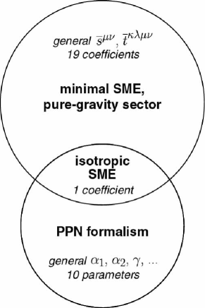
Figure 1: Schematic relationship between the pure-gravity sector of the minimal SME and the PPN formalism.

The relationship between the pure-gravity sector of the minimal SME and the PPN formalism can be represented as the Venn diagram in Fig. 1. The overlap region, which corresponds to the isotropic limit, is a one-parameter region in the universe rest frame. This overlap region encompasses only a small portion of the effects governed by the pure-gravity sector of the minimal SME and by the PPN formalism. Much experimental work has been done to explore the PPN parameters. However, the figure illustrates that a large portion of coefficient space associated with dominant effects in a realistic action (SME) remains open for experimental exploration. We initiate the theoretical investigation of the various possible experimental searches for these effects in Sec. V.

We note in passing that the above matching considerations are derived for the pure-gravity sector of the minimal SME. However, even in the isotropic limit, the matter sector of the minimal SME contains numerous additional coefficients for Lorentz violation. Attempting a match between the isotropic limit of the minimal SME with matter and the PPN formalism would also be of interest but lies beyond our present scope.

III.3.2 Anisotropic-universe model

An approach adopting a somewhat different philosophy is the anisotropic-universe model nanis . This model is conservative and is based on the formulation of an effective classical point-particle lagrangian. Possible anisotropies in a preferred frame are parametrized via a set of spatial two-tensors and spatial vectors, and the post-newtonian metric is constructed. The model includes velocity-dependent terms and three-body interactions up to $O(4)$. The connection to the PPN formalism is discussed in Ref. nanis .

A detailed match between the anisotropic-universe model and the classical point-particle limit of the pure-gravity sector of the minimal SME is impractical at present, since the $O(4)$ terms for the latter are undetermined. However, some suggestive features of the relationship can be obtained. For this purpose, it suffices to consider the restriction of the anisotropic-universe model to two-body terms at $O(3)$. In this limit, the lagrangian is

$$L_{\rm AU} = {\textstyle{{1}\over{2}}}\sum_{a}m_{a}\vec{v}^{2}_{a}+{\textstyle{{1}\over{2}}}\sum_{ab}{{Gm_{a}m_{b}}\over{r_{ab}}}(1+2\Omega^{jk}\hat{r}^{j}_{ab}\hat{r}^{k}_{ab})$$ (74)

$$+\sum_{ab}{{Gm_{a}m_{b}}\over{r_{ab}}}(\Phi^{j}v^{j}_{a}+\Upsilon^{j}\hat{r}^{j}_{ab}v^{k}_{a}\cdot\hat{r}^{k}_{ab}).$$

The anisotropic properties of the model at this order are controlled by 11 parameters, collected into one symmetric spatial two-tensor $\Omega^{jk}$ and two three-vectors $\Phi^{j}$, $\Upsilon^{j}$.

To gain insight into the relationship, we can compare Eq. (74) with the $O(3)$ point-particle lagrangian (54) obtained in Sec. III.2. Consider the match in the preferred frame of the anisotropic-universe model. Comparison of Eqs. (74) and (54) gives the correspondence

$$\Omega^{jk} = {\textstyle{{1}\over{4}}}\overline{s}^{jk}-{\textstyle{{1}\over{12}}}\overline{s}^{00}\delta^{jk},$$

$$\Phi^{j} = -{\textstyle{{3}\over{2}}}\overline{s}^{0j},$$

$$\Upsilon^{j} = -{\textstyle{1\over 2}}\overline{s}^{0j}.$$ (75)

The five parameters $\Omega^{jk}$ are determined by the SME coefficients $\overline{s}^{jk}$ and $\overline{s}^{00}$, while the two three-vectors $\Phi^{j}$, $\Upsilon^{j}$ are determined by $\overline{s}^{0j}$.

The SME is a complete effective field theory and so contains effects beyond any point-particle description, including that of the anisotropic-universe model. Even in the point-particle limit, it is plausible that the pure-gravity sector of the minimal SME describes effects outside the anisotropic-universe model because the latter is based on two-tensors and vectors while the SME contains the four-tensor $\overline{t}^{\kappa\lambda\mu\nu}$. Nonetheless, in this limit the converse is also plausible: the anisotropic-universe model is likely to contain effects outside the pure-gravity sector of the minimal SME. The point is that the match (75) implies the 11 parameters $\Omega^{jk}$, $\Phi^{j}$, $\Upsilon^{j}$ are fixed by only 9 independent SME coefficients $\overline{s}^{\mu\nu}$. This suggests that two extra degrees of freedom appear in the anisotropic-universe model already at $O(3)$. Some caution with this interpretation may be advisable, as the condition $\Phi^{j}=3\Upsilon^{j}$ implied by Eq. (75) in the context of the minimal SME arises from the requirement that the form of the lagrangian be observer invariant under post-galilean transformations. To our knowledge the observer transformation properties of the parameters in the anisotropic-universe model remain unexplored in the literature, and adding this requirement may remove these two extra degrees of freedom. At $O(4)$, however, the full anisotropic-universe model contains additional two-tensors for which there are no matching additional coefficients in the pure-gravity sector of the minimal SME. It therefore appears likely that the correspondence between the two approaches is again one of partial overlap. It is conceivable that effects from the SME matter sector or from nonminimal SME terms could produce a more complete correspondence.

IV Illustration: bumblebee models

The analysis presented in Secs. II and III applies to all theories with terms for Lorentz violation that can be matched to the general form (5). An exploration of its implications for experiments is undertaken in Sec. V. Here, we first take a short detour to provide a practical illustration of the general methodology and to illuminate the role of the five assumptions adopted in the linearization procedure of Sec. II.2. For this purpose, we consider a specific class of theories, the bumblebee models. Note, however, that the material in this section is inessential for the subsequent analysis of experiments, which is independent of specific models. The reader can therefore proceed directly to Sec. V at this stage if desired.

Bumblebee models are theories involving a vector field $B^{\mu}$ that have spontaneous Lorentz violation induced by a potential $V(B^{\mu})$. The action relevant for our present purposes can be written as

$$S_{B} = \int d^{4}x\Big{[}{{1}\over{2\kappa}}(eR+\xi eB^{\mu}B^{\nu}R_{\mu\nu})$$ (76)

$$\hskip-10.0pt\phantom{\int d^{4}x}-{\textstyle{{1}\over{4}}}\alpha eB^{\mu\nu}B_{\mu\nu}+{\textstyle{{1}\over{2}}}\beta e(D_{\mu}B_{\nu})(D^{\mu}B^{\nu})$$

$$\hskip-10.0pt\phantom{\int d^{4}x}-eV(B^{\mu})+{\cal L}_{\rm M}\Big{]},$$

where $\alpha$ and $\beta$ are real. In Minkowski spacetime and with vanishing potential $V$, a nonzero value of $\beta$ introduces a Stückelberg ghost. However, the ghost term with $\beta$ potentially nonzero is kept in the action here to illustrate some features of the assumptions made in Sec. II.2. In Eq. (76), the potential $V$ is taken to have the functional form

$$V(B^{\mu})=V(B^{\mu}B_{\mu}\pm b^{2}),$$ (77)

where $b^{2}$ is a real number. This potential induces a nonzero vacuum value $B^{\mu}=b^{\mu}$ obeying $b^{\mu}b_{\mu}=\mp b^{2}$. The theory (76) is understood to be taken in the limit of Riemann spacetime, where the field-strength tensor can be written as $B_{\mu\nu}=\partial_{\mu}B_{\nu}-\partial_{\nu}B_{\mu}$. Bumblebee models involving nonzero torsion in the more general context of Riemann-Cartan spacetime are investigated in Refs. akgrav ; bkgrav .

Theories coupling gravity to a vector field with a vacuum value have a substantial history in the literature. A vacuum value as a gauge choice for the photon was discussed by Nambu nambu . Models of the form (76) without a potential term but with a vacuum value for $B^{\mu}$ and nonzero values of $\alpha$ and $\beta$ were considered by Will and Nordtvedt wn and by Hellings and Nordtvedt hn . The idea of using a potential $V$ to break Lorentz symmetry spontaneously and hence to enforce a nonzero vacuum value for $B^{\mu}$ was introduced by Kostelecký and Samuel ks2 , who studied both the smooth ‘quadratic’ case $V=-\lambda e(B^{\mu}B_{\mu}\pm b^{2})^{2}/2$ and the limiting Lagrange-multiplier case $V=-\lambda e(B^{\mu}B_{\mu}\pm b^{2})$ for $\beta=0$ and in $N$ dimensions. The spontaneous Lorentz breaking is accompanied by qualitatively new features, including a Nambu-Goldstone sector of massless modes bkgrav , the necessary breaking of U(1) gauge invariance akgrav , and implications for the behavior of the matter sector kleh , the photon bkgrav , and the graviton akgrav ; kpssb . More general potentials have also been investigated, and some special cases with hypergeometric $V$ turn out to be renormalizable in Minkowski spacetime aknonpoly . The situation with a Lagrange-multiplier potential for a timelike $b_{\mu}$ and both $\alpha$ and $\beta$ nonzero has been explored by Jacobson and collaborators jm . Related analyses have been performed in Refs. bb1 ; bb2 .

In what follows, we consider the linearized and post-newtonian limits of the theory (76) for some special cases. The action for the theory contains a pure-gravity Einstein piece, a gravity-bumblebee coupling term controlled by $\xi$, several terms determining the bumblebee dynamics, and a matter Lagrange density. Comparison of Eq. (76) with the action (5) suggests a correspondence between the gravity-bumblebee coupling and the fields $u$ and $s^{\mu\nu}$, with the latter being related to the traceless part of the product $B^{\mu}B^{\nu}$. It is therefore reasonable to expect the linearization analysis of the previous sections can be applied, at least for actions with appropriate bumblebee dynamics.

IV.1 Cases with $\beta=0$

Consider first the situation without a ghost term, $\beta=0$. Suppose for definiteness that $\alpha=1$. The modified Einstein and bumblebee field equations for this case are given in Ref. akgrav . To apply the general formalism developed in the previous sections, we first relate the bumblebee action (76) to the action (3) of the pure-gravity sector of the minimal SME, and then we consider the linearized version of the equations of motion.

The match between the bumblebee and SME actions involves identifying $u$ and $s^{\mu\nu}$ as composite fields of the underlying bumblebee field and the metric, given by

$$u = {\textstyle{{1}\over{4}}}\xi B^{\alpha}B^{\beta}g_{\alpha\beta},$$

$$s^{\mu\nu} = \xi B^{\mu}B^{\nu}-{\textstyle{{1}\over{4}}}\xi B^{\alpha}B^{\beta}g_{\alpha\beta}g^{{\mu\nu}}.$$ (78)

This is a nonlinear relationship between the basic fields of a given model and the SME, a possibility noted in Sec. II.1.

Following the notation of Sec. II.2, the bumblebee field $B^{\mu}$ can be expanded around its vacuum value $b^{\mu}$ as

$$B^{\mu}=b^{\mu}+\tilde{B}^{\mu}.$$ (79)

In an asympotically cartesian coordinate system, the vacuum value is taken to obey

$$\partial_{\nu}b^{\mu}=0.$$ (80)

This ensures that assumption (i) of Sec. II.2 holds.

The expansion of the SME fields $u$, $s^{\mu\nu}$, $t^{\kappa\lambda{\mu\nu}}$ about their vacuum values is given in Eq. (10). At leading order, the $\xi$-dependent term in the bumblebee action (76) is reproduced by the Lorentz-violating piece (5) of the SME action by making the identifications

$$\overline{u} = {\textstyle{{1}\over{4}}}\xi b^{\alpha}b_{\alpha},$$

$$\tilde{u} = {\textstyle{1\over 2}}\xi(b_{\alpha}\tilde{B}^{\alpha}+{\textstyle{1\over 2}}b^{\alpha}b^{\beta}h_{\alpha\beta}),$$

$$\overline{s}^{\mu\nu} = \xi(b^{\mu}b^{\nu}-{\textstyle{{1}\over{4}}}\eta^{\mu\nu}b^{\alpha}b_{\alpha}),$$

$$\tilde{s}^{\mu\nu} = \xi(b^{\mu}\tilde{B}^{\nu}+b^{\nu}\tilde{B}^{\mu}+{\textstyle{{1}\over{4}}}h^{\mu\nu}b^{\alpha}b_{\alpha}$$

$$\phantom{\xi}-{\textstyle{{1}\over{2}}}\eta^{\mu\nu}b_{\alpha}\tilde{B}^{\alpha}-{\textstyle{{1}\over{4}}}\eta^{\mu\nu}b^{\alpha}b^{\beta}h_{\alpha\beta}),$$

$$\overline{t}^{\kappa\lambda\mu\nu} = 0,$$

$$\tilde{t}^{\kappa\lambda\mu\nu} = 0.$$ (81)

We see that assumption (ii) of Sec. II.2 holds if the combination $\xi b^{\mu}b^{\nu}$ is small.

The next step is to examine the field equations. The nonlinear nature of the match (78) and its dependence on the metric imply that the direct derivation of the linearized effective Einstein equations from the bumblebee theory (76) differs in detail from the derivation of the same equations in terms of $s^{\mu\nu}$ and $u$ presented in Sec. II.2. For illustrative purposes and to confirm the results obtained via the general linearization process, we pursue the direct route here.

Linearizing in both the metric fluctuation $h_{\mu\nu}$ and the bumblebee fluctuation $\tilde{B}^{\mu}$ but keeping all powers of the vacuum value $b^{\mu}$, the linearized Einstein equations can be extracted from the results of Ref. akgrav . Similarly, the linearized equations of motion for the bumblebee fluctuations can be obtained. For simplicity, we disregard the possibility of direct couplings between the bumblebee fields and the matter sector, which means that assumption (iii) of Sec. II.2 holds. The bumblebee equations of motion then take the form

$$\partial^{\mu}B_{\mu\nu}=2V^{\prime}b_{\nu}-{\textstyle{{\xi}\over{\kappa}}}b^{\mu}R_{\mu\nu},$$ (82)

where the prime denotes the derivative with respect to the argument. Once the potential $V$ is specified, Eq. (82) for the bumblebee fluctuations can be inverted using Fourier decomposition in momentum space.

Consider, for example, the situation for a smooth potential $V=-\lambda e(B^{\mu}B_{\mu}\pm b^{2})^{2}/2$. For this case, Eq. (82) can be written as

$$(\eta_{\mu\nu}\Box-\partial_{\mu}\partial_{\nu}-4\lambda b_{\mu}b_{\nu})\tilde{B}^{\mu}=$$

$$-b^{\alpha}\partial^{\mu}(\partial_{\mu}h_{\nu\alpha}-\partial_{\nu}h_{\mu\alpha})+2\lambda b_{\nu}b^{\alpha}b^{\beta}h_{\alpha\beta}-{\textstyle{{\xi}\over{\kappa}}}b^{\alpha}R_{\alpha\nu}.$$

(83)

Converting to momentum space, the propagator for the $\tilde{B}^{\mu}$ field for both timelike and spacelike $b^{\mu}$ is found to be

$$G^{\mu\nu}(p) = -{{\eta^{\mu\nu}}\over{p^{2}}}+{{(b^{\mu}p^{\nu}+b^{\nu}p^{\mu})}\over{p^{2}b_{\alpha}p^{\alpha}}}$$ (84)

$$\qquad\qquad-{{(4\lambda b^{\alpha}b_{\alpha}+p^{2})p^{\nu}p^{\mu}}\over{4\lambda p^{2}(b_{\alpha}p^{\alpha})^{2}}}.$$

In this equation, $p^{\mu}$ is the four momentum and $p^{2}\equiv p^{\mu}p_{\mu}$. This propagator matches results from other analyses aknonpoly ; bb1 .

The propagator (84) can be used to solve for the harmonic bumblebee fluctuation $\tilde{B}^{\mu}(p)$ in momentum space in terms of the metric. We find

$$\tilde{B}^{\mu}(p) = -h^{\mu\alpha}b_{\alpha}+{{p^{\mu}b^{\alpha}b^{\beta}h_{\alpha\beta}}\over{2b^{\alpha}p_{\alpha}}}$$ (85)

$$-{{\xi b^{\mu}R}\over{2\kappa p^{2}}}+{{\xi p^{\mu}R}\over{8\kappa\lambda b^{\alpha}p_{\alpha}}}+{{\xi p^{\mu}b^{\alpha}b_{\alpha}R}\over{2\kappa p^{2}b^{\alpha}p_{\alpha}}}$$

$$+{{\xi b_{\alpha}R^{\alpha\mu}}\over{\kappa p^{2}}}-{{\xi p^{\mu}b^{\alpha}b^{\beta}R_{\alpha\beta}}\over{\kappa p^{2}b^{\alpha}p_{\alpha}}}.$$

This solution can be reconverted to position space and substituted into the linearized gravitational field equations to generate the effective Einstein equations for $h_{\mu\nu}$. At leading order in the coupling $\xi$, these take the expected general form (23) with the identifications in Eq. (81), except that the coefficient of $\Phi^{\overline{u}}_{\mu\nu}$ appears as $-3$ rather than unity. To match the normalization conventions adopted in Eq. (23), a rescaling of the type discussed in Sec. II.2 must be performed, setting $\overline{u}\rightarrow-\overline{u}/3$. The calculation shows that assumption (v) in Sec. II.2 holds. Moreover, the independently conserved piece $\Sigma_{\mu\nu}$ of the energy-momentum tensor $(S_{stu})_{\mu\nu}$ contains only a trace term generating the rescaling of $\Phi^{\overline{u}}_{\mu\nu}$. This bumblebee theory therefore provides an explicit illustration of a model that weakly violates assumption (iv) of Sec. II.2.

A similar analysis can be performed for the Lagrange-multiplier potential $V=-\lambda e(B^{\mu}B_{\mu}\pm b^{2})$, for both timelike and spacelike $b^{\mu}$. We find that the linearized limits of these models are also correctly described by the general formalism developed in the previous sections, including the five assumptions of Sec. II.2.

It follows that the match (71) to the PPN formalism holds for all these bumblebee models in the context of the isotropic limit, for which $b^{0}$ is the only nonzero coefficient in the universe rest frame. Note that the condition (72) is valid both for the Lagrange-multiplier potential and for the smooth potential. In fact, the $\beta=0$ model with zero potential term $V=0$ but a nonzero isotropic vacuum value for $B^{\mu}$ also satisfies the condition (72) at leading order hn ; cmw .

We note in passing that the limit of zero coupling $\xi$ implies the vanishing of all the coefficients and fluctuations in Eq. (81). In the pure gravity-bumblebee sector, any Lorentz-violating effects in the effective linearized theory must then ultimately be associated with the bumblebee potential $V$. Within the linearization assumptions we have made above, this result is compatible with that obtained in Ref. bkgrav for the effective action of the bumblebee Nambu-Goldstone fluctuations, for which the Einstein-Maxwell equations are recovered in the same limit. Further insight can be obtained by examining the bumblebee trace-reversed energy-momentum tensor $(S_{B})_{\mu\nu}$, obtained by varying the minimally coupled parts of the bumblebee action (76) with respect to the metric. This variation gives

$$(S_{B})_{\mu\nu} = b_{\mu}\partial^{\alpha}B_{\alpha\nu}+b_{\nu}\partial^{\alpha}B_{\alpha\mu}-\eta_{\mu\nu}b^{\beta}\partial^{\alpha}B_{\alpha\beta}$$ (86)

$$-2(b_{\mu}b_{\nu}-{\textstyle{{1}\over{2}}}\eta_{\mu\nu}b^{\alpha}b_{\alpha})V^{\prime}.$$

Note that the composite nature of $u$ and $s^{\mu\nu}$ means that this expression cannot be readily identified with any of the various pieces of the energy-momentum tensor introduced in Sec. II.2. Using the bumblebee field equations, $(S_{B})_{\mu\nu}$ can be expressed entirely in terms of $V^{\prime}$ and terms proportional to $\xi$, whatever the chosen potential. For the smooth quadratic potential, insertion of the bumblebee modes $\tilde{B}^{\mu}$ obtained in Eq. (85) yields

$$V^{\prime} = \lambda(2b^{\alpha}\tilde{B}_{\alpha}+b^{\alpha}b^{\beta}h_{\alpha\beta})={{\xi R}\over{4\kappa}}.$$ (87)

This shows that all terms in $(S_{B})_{\mu\nu}$ are proportional to $\xi$, thereby confirming that these modes contribute no Lorentz-violating effects to the behavior of $h_{\mu\nu}$ in the limit of vanishing $\xi$. Appropriate calculations for the analogous modes of $\tilde{B}^{\mu}$ in the case of the Lagrange-multiplier potential gives the same result.

IV.2 Cases with $\beta\neq 0$

As an example of a model that lies within the minimal SME but outside the mild assumptions of Sec. II.2, consider the limit $\alpha=0$ and $\beta=1$ of the theory (76). The kinetic term of this theory is expected to include negative-energy contributions from the ghost term.

Following the path adopted in Sec. IV.1, we expand the bumblebee field about its vacuum value as in Eq. (79), impose the condition (80) of asymptotic cartesian constancy, make the identifications (81), and disregard bumblebee couplings to the matter sector. It then follows that the limit $\alpha=0$, $\beta=1$ also satisfies assumptions (i), (ii) and (iii) of Sec. II.2. In this limit, the bumblebee equations of motion become

$$D^{\mu}D_{\mu}B_{\nu}=2V^{\prime}b_{\nu}-{\textstyle{{\xi}\over{\kappa}}}b^{\mu}R_{\mu\nu}.$$ (88)

For specific potentials, the linearized form of Eq. (88) can be inverted by Fourier decomposition and the propagator obtained. Here, we consider for definiteness the potential $V=-\lambda e(B^{\mu}B_{\mu}\pm b^{2})^{2}/2$. However, most of the results that follow also hold for the Lagrange-multiplier potential.

Inverting and substituting into the linearized modified Einstein equations produces the effective equations for $h_{\mu\nu}$. For our purposes, it suffices to study the case $\xi=0$. In the harmonic gauge, we find the perturbation $h_{\mu\nu}$ is determined by the linearized effective equations

$$R_{\mu\nu} = \kappa[{\textstyle{{1}\over{2}}}b^{\alpha}b_{(\mu}\Box h_{\nu)\alpha}-{\textstyle{{1}\over{2}}}b^{\alpha}b^{\beta}\partial_{\alpha}\partial_{(\mu}h_{\nu)\beta}$$ (89)

$$+{\textstyle{{1}\over{2}}}(b^{\alpha}\partial_{\alpha})^{2}h_{\mu\nu}-{\textstyle{{1}\over{4}}}b^{\alpha}b_{(\mu}\partial_{\nu)}\partial_{\alpha}h^{\gamma}_{\phantom{\gamma}\gamma}$$

$$-{\textstyle{{1}\over{4}}}\eta_{\mu\nu}b^{\alpha}b^{\beta}\Box h_{\alpha\beta}+(S_{M})_{\mu\nu}].$$

The right-hand side of this equation fails to match the generic form (23) of the linearized equations derived in Sec. II.2. In fact, the non-matter part can be regarded as an effective contribution to the independently conserved piece $\Sigma_{\mu\nu}$ of the energy-momentum tensor $(S_{stu})_{\mu\nu}$. We can therefore conclude that the ghost model with $\alpha=0$, $\beta=1$ strongly violates assumption (iv) of Sec. II.2.

The ghost nature of the bumblebee modes in this model implies that an exploration of propagating solutions of Eq. (89) can be expected to encounter problems with negative energies. Nonetheless, a post-newtonian expansion for the metric can be performed. For definiteness, we take the effective coefficients for Lorentz violation $\kappa b^{\mu}b^{\nu}$ to be small, and we adopt the isotropic-limit assumption that in the universe rest frame only the coefficient $b^{0}$ is nonzero. A calculation then reveals that the post-newtonian metric at $O(3)$ in the Sun-centered frame and in the gauge (34) is given by

$$g_{00} = -1+2U-\kappa(b^{0})^{2}w^{2}U+\kappa(b^{0})^{2}w^{j}w^{k}U^{jk}$$

$$-2\kappa(b^{0})^{2}w^{j}(V^{j}-W^{j})+O(4),$$

$$g_{0j} = -{\textstyle{{7}\over{2}}}V^{j}-{\textstyle{{1}\over{2}}}W^{j},$$

$$g_{jk} = \delta^{jk}(1+2U),$$ (90)

where $G$ has been appropriately rescaled. Comparison with the PPN metric (59) in the same gauge yields the following parameter values in this ghost model:

$$\alpha_{1} = 0,$$

$$\alpha_{2} = -\kappa(b^{0})^{2},$$

$$\alpha_{3} = 0,$$

$$\gamma = 1.$$ (91)

This model therefore fails to obey the condition (72). The violation of assumption (iv) evidently affects the general structure of the post-newtonian metric.

In light of the results obtained above, we conjecture that quadratic ghost kinetic terms are associated with a nonzero value of $\Sigma_{\mu\nu}$ that strongly violates assumption (iv) of Sec. II.2 and that violates the condition (72) at linear order in the isotropic limit. This conjecture is consistent with the results obtained above with the Lagrange-multiplier potential and with the smooth potential, both for the case $\beta=0$ and for the case $\beta\neq 0$. Moreover, studies in the context of the PPN formalism of various models with $V=0$ but a nonzero vacuum value for $B^{\mu}$ also suggest that ghost terms are associated with violations of the condition (72). For example, this is true of the post-newtonian limit of the ghost model with vanishing $V=0$ and $\xi=0$ wn . Similarly, inspection of the general case with $V=0$ but $\alpha\neq 0$ and $\beta\neq 0$ cmw shows that the condition (72) is satisfied at linear order in the PPN parameters when $\beta$ vanishes. A proof of the conjecture in the general context appears challenging to obtain but would be of definite interest.

V Experimental Applications

The remainder of this paper investigates various gravitational experiments to determine signals for nonzero coefficients for Lorentz violation and to estimate the attainable sensitivities. The dominant effects of Lorentz violation in these experiments are associated with newtonian $O(2)$ and post-newtonian $O(3)$ terms in $g_{00}$ and with post-newtonian $O(2)$ terms in $g_{0j}$. They are controlled by combinations of the 9 coefficients $\overline{s}^{\mu\nu}$. Effects from $O(4)$ terms in $g_{00}$ lie beyond the scope of the present analysis. However, some effects involving $O(3)$ terms in $g_{0j}$ or $O(2)$ terms in $g_{jk}$ are accessible by focusing on specific measurable signals. For example, experiments involving the classic time-delay effect on a photon passing near a massive body or the spin precession of a gyroscope in curved spacetime can achieve sensitivity to terms at these orders.

We begin in Sec. V.1 with a discussion of our frame conventions and transformation properties, which are applicable to many of the experimental scenarios considered below. The types of experimental constraints that might be deduced from prior experiments are also summarized. The remaining subsections treat distinct categories of experiments. Section V.2 examines measurements obtained from lunar and satellite laser ranging. Section V.3 considers terrestrial experiments involving gravimeter and laboratory tests. Orbiting gyroscopes provide another source of information, as described in Sec. V.4. The implications for Lorentz violation of observations of binary-pulsar systems are discussed in Sec. V.5. The sensitivies of the classic tests, in particular the perihelion shift and the time-delay effect, are considered in Sec. V.6. More speculative applications of the present theory, for example to the properties of dark matter or to the Pioneer anomaly, are also of interest but their details lie beyond the scope of this work and will be considered elsewhere.

V.1 General Considerations

V.1.1 Frame conventions and transformations

The comparative analysis of signals for Lorentz violation from different experiments is facilitated by adopting a standard inertial frame. The canonical reference frame for SME experimental studies in Minkowski spacetime is a Sun-centered celestial-equatorial frame km . In the present context of post-newtonian gravity, the standard inertial frame is chosen as an asymptotically inertial frame that is comoving with the rest frame of the solar system and that coincides with the canonical Sun-centered frame. The cartesian coordinates in the Sun-centered frame are denoted by

$$x^{\Xi}=(T,X^{J})=(T,X,Y,Z)$$ (92)

and are labeled with capital Greek letters. By definition, the $Z$ axis is aligned with the rotation axis of the Earth, while the $X$ axis points along the direction from the center of the Earth to the Sun at the vernal equinox. The inclination of the Earth’s orbit is denoted $\eta$. The origin of the coordinate time $T$ is understood to be the time when the Earth crosses the Sun-centered $X$ axis at the vernal equinox. This standard coordinate system is depicted in Fig. 2. The corresponding coordinate basis vectors are denoted

$${\bf e}_{\Xi}=({\bf e}_{T},{\bf e}_{J})=(\partial_{T},\partial_{J}).$$ (93)

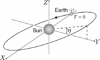
Figure 2: Sun-centered celestial-equatorial frame.

In the Sun-centered frame, as in any other inertial frame, the post-newtonian spacetime metric takes the form given in Eqs. (LABEL:g00)-(LABEL:gjk). This metric, along with the point-mass equations of motion (52), forms the basis of our experimental studies to follow. The corresponding line element can be written in the form

$$ds^{2} = -[1-h_{TT}(T,\vec{X})+O(4)]dT^{2}$$ (94)

$$+2h_{TJ}(T,\vec{X})dTdX^{J}$$

$$+[\delta_{JK}+h_{JK}(T,\vec{X})]dX^{J}dX^{K},$$

where $h_{TT}$ is taken to $O(3)$, $h_{TJ}$ is taken to $O(3)$ and $h_{JK}$ is taken to $O(2)$. For the purposes of this work, it typically suffices to include contributions to the metric fluctuations from the Sun and the Earth.

Of particular interest for later applications are various sets of orthonormal basis vectors that can be defined in the context of the line element (94). One useful set is appropriate for an observer at rest, $dX^{J}/dT=0$, at a given point $(T,\vec{X})$ in the Sun-centered frame. Denoting the four elements of this basis set by ${\bf e}_{\mu}$ with $\mu\equiv(t,j)$, we can write

$${\bf e}_{t} = \delta_{\phantom{T}t}^{T}[1+{\textstyle{{1}\over{2}}}h_{TT}(T,\vec{X})+O(4)]{\bf e}_{T},$$

$${\bf e}_{j} = \delta^{J}_{\phantom{J}j}[{\bf e}_{J}-{\textstyle{{1}\over{2}}}h_{JK}(T,\vec{X}){\bf e}_{K}]+\delta^{J}_{\phantom{J}j}h_{TJ}(T,\vec{X}){\bf e}_{T}.$$

Direct calculation shows that this basis satisfies

$$ds^{2}=-{\bf e}_{t}^{2}+{\bf e}_{j}^{2}$$ (96)

to post-newtonian order.

Another useful set of basis vectors, appropriate for an observer in arbitrary motion, can be obtained from the basis set (LABEL:ortho1) by applying a local Lorentz transformation. Denoting this new set of vectors by ${\bf e}_{\hat{\mu}}$, we have

$${\bf e}_{\hat{\mu}}=\Lambda^{\nu}_{\phantom{\nu}\hat{\mu}}(\tau){\bf e}_{\nu}.$$ (97)

It is understood that all quantities on the right-hand side of this equation are to be evaluated along the observer’s worldline, which is parametrized by proper time $\tau$.

For the experimental applications in the present work, it suffices to expand the local Lorentz transformation in Eq. (97) in a post-newtonian series. This gives

$${\bf e}_{\hat{t}} = \delta^{t}_{\phantom{t}\hat{t}}(1+{\textstyle{{1}\over{2}}}v^{2}){\bf e}_{t}+v^{j}{\bf e}_{j},$$

$${\bf e}_{\hat{j}} = \delta^{j}_{\phantom{j}\hat{j}}v^{k}R^{kj}{\bf e}_{t}+\delta^{j}_{\phantom{j}\hat{j}}(\delta^{kl}+{\textstyle{{1}\over{2}}}v^{k}v^{l})R^{lj}{\bf e}_{k}.$$ (98)

The components $({\bf e}_{\hat{t}})^{\Xi}$ coincide with the observer’s four-velocity $u^{\Xi}$ in the Sun-centered frame. In this expression, $v^{j}$ is the coordinate velocity of the observer as measured in the frame (LABEL:ortho1), and $R^{jk}$ is an arbitrary rotation. The reader is cautioned that the coordinate velocities $v^{j}$ and $v^{J}$ typically differ at the post-newtonian level. The explicit relationship can be derived from (LABEL:ortho1) and is found to be

$$v^{j}=\delta_{J}^{\phantom{J}j}v^{J}(1+{\textstyle{{1}\over{2}}}h_{TT})+{\textstyle{{1}\over{2}}}\delta_{J}^{\phantom{J}j}h_{JK}v^{K}+O(4).$$ (99)

V.1.2 Current bounds

In most modern tests of local Lorentz symmetry with gravitational experiments, the data have been analyzed in the context of the PPN formalism. The discussion in Sec. III.3 shows there is a correspondence between the PPN formalism and the pure-gravity sector of the minimal SME in a special limit, so it is conceivable a priori that existing data analyses could directly yield partial information about SME coefficients. Moreover, a given experiment might in fact have sensitivity to one or more SME coefficients even if the existing data analysis fails to identify it, so the possibility arises that new information can be extracted from available data by adopting the SME context. The specific SME coefficients that could be measured by the reanalysis of existing experiments depend on details of the experimental procedure. Nonetheless, a general argument can be given that provides a crude estimate of the potential sensitivities and the SME coefficients that might be constrained.

The standard experimental analysis for Lorentz violation in gravitational experiments is based on the assumed existence of a preferred-frame vector $\vec{w}$. Usually, this is taken to have a definite magnitude and orientation for the solar system and is identified with the velocity of the solar system with respect to the rest frame of the cosmic microwave background radiation cmw . The strength of the coupling of the vector to gravity is then determined by the two PPN parameters $\alpha_{1}$ and $\alpha_{2}$.

Performing a data analysis of this type under the assumption that the vector $\vec{w}$ is the source of isotropy violations is equivalent in the SME context to supposing that only parallel projections of the coefficients $\overline{s}^{\mu\nu}$ along the unit vector $\hat{w}$ contribute to any signals. This holds regardless of the choice of $\vec{w}$. For the coefficients $\overline{s}^{\mu\nu}$, there are two possible parallel projections, given by

$$\overline{s}^{0j}_{\parallel} = \hat{w}^{j}\hat{w}^{k}\overline{s}^{0k},$$

$$\overline{s}^{jk}_{\parallel} = \hat{w}^{j}\hat{w}^{k}\hat{w}^{l}\hat{w}^{m}\overline{s}^{lm}.$$ (100)

Also, the coefficients $\overline{t}^{\kappa\lambda\mu\nu}$ play no role in the analysis at this order, in accordance with the discussion in Sec. II.2.4. It therefore follows that sensitivity to at most 2 of the 19 SME coefficients $\overline{s}^{\mu\nu}$ and $\overline{t}^{\kappa\lambda\mu\nu}$ could be extracted from these types of analyses of experimental data. Together with the 10 coefficients $\overline{t}^{\kappa\lambda\mu\nu}$, the 7 perpendicular projections given by

$$\overline{s}^{0j}_{\perp} = \overline{s}^{0k}-\hat{w}^{j}\hat{w}^{k}\overline{s}^{0k},$$

$$\overline{s}^{jk}_{\perp} = \overline{s}^{jk}-\hat{w}^{j}\hat{w}^{k}\hat{w}^{l}\hat{w}^{m}\overline{s}^{lm}$$ (101)

remain unexplored in experimental analyses to date.

The two independent measurements of parallel projections of SME coefficients could be obtained, for example, from a reanalysis of existing data from lunar laser ranging al1llr ; al2llr . A crude estimate of the sensitivity to be expected can be obtained by assuming that the bounds attained on a particular term of the PPN metric in the Sun-centered frame roughly parallel those that might be achieved for the corresponding term in the pure-gravity minimal-SME metric. This procedure gives $\overline{s}^{0j}_{\parallel}\mathrel{\hbox to0.0pt{\lower 4.0pt\hbox{\hskip 1.0pt$\sim$}\hss}\raise 1.0pt\hbox{$<$}}10^{-8}$ and $\overline{s}^{jk}_{\parallel}\mathrel{\hbox to0.0pt{\lower 4.0pt\hbox{\hskip 1.0pt$\sim$}\hss}\raise 1.0pt\hbox{$<$}}10^{-11}$. However, these estimates are untrustworthy because the substantial differences between the two metrics imply unknown effects on the data analysis, so these constraints are no more than a guide to what might be achieved.

A more interesting constraint can be obtained by considering implications of the observed close alignment of the Sun’s spin axis with the angular-momentum axis of the planetary orbits. The key point is that the metric term $\overline{s}^{jk}U^{jk}$ violates angular-momentum conservation. As a result, a spinning massive body experiences a self-torque controlled by the coefficients $\overline{s}^{jk}$. For the Sun, this effect induces a precession of the spin axis, which over the lifetime of the solar system would produce a misalignment of the spin axis relative to the ecliptic plane. This idea was introduced by Nordtvedt and used to bound the PPN parameter $\alpha_{2}$ nsol . In the context of the pure-gravity sector of the minimal SME, the analysis is similar and so is not presented here. It turns out that the final result involves a particular combination of SME coefficients in the Sun-centered frame given by

$$\overline{s}_{\rm SSP} = \sqrt{\overline{s}_{\rm t}^{JK}\overline{s}_{\rm t}^{JL}\hat{S}^{K}\hat{S}^{L}-(\overline{s}_{\rm t}^{JK}\hat{S}^{J}\hat{S}^{K})^{2}}.$$ (102)

In this expression, $\hat{S}^{J}$ are the Sun-frame components of the unit vector pointing in the direction of the present solar spin. The coefficients $\overline{s}_{\rm t}^{JK}$ are the traceless components of $\overline{s}^{JK}$, given by

$$\overline{s}_{\rm t}^{JK}=\overline{s}^{JK}-{\textstyle{{1}\over{3}}}\delta^{JK}\overline{s}^{TT}.$$ (103)

Under the assumption that the coefficients $\overline{s}_{\rm t}^{JK}$ are small enough for perturbation theory to be valid, we find an approximate bound of $\overline{s}_{\rm SSP}\mathrel{\hbox to0.0pt{\lower 4.0pt\hbox{\hskip 1.0pt$\sim$}\hss}\raise 1.0pt\hbox{$<$}}10^{-13}$.

V.2 Lunar and Satellite Ranging

Lunar laser ranging is among the most sensitive tests of gravitational physics within the solar system to date. Dominant orbital perturbations in the context of the PPN metric were obtained in Ref. nllr , while oscillations arising from a subset of the parameters for the anisotropic-universe model were calculated in Ref. nanisllr . Here, we obtain the dominant effects on the motion of a satellite orbiting the Earth that arise from nonzero coefficients $\overline{s}^{\mu\nu}$ for Lorentz violation. Our results are applicable to the Earth-Moon system as well as to artificial satellites.

The analysis is performed in the Sun-centered frame. The satellite motion is affected by the Earth, the Sun, and other perturbing bodies. For the analysis, it is useful to introduce quantities to characterize the masses, positions, sidereal frequencies, etc., relevant for the motion. These are listed in Table 1. The various position vectors are depicted in Fig. 3.

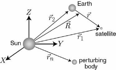
Figure 3: The Earth-satellite system in the Sun-centered frame.

This subsection begins by presenting the coordinate acceleration of the Earth-satellite separation, which is the primary observable in laser-ranging experiments. To gain insight into the content of the resulting expressions, we next perform a perturbative analysis that extracts the dominant frequencies and corresponding amplitudes for oscillations driven by Lorentz violation. This analysis is somewhat lengthy, and it is largely relegated to Appendix A, with only the primary results presented in the main text. Finally, we estimate the likely sensitivities attainable in experimental analyses of ranging to the Moon and to various artificial satellites.

Quantity	Definition
$m_{1}$	satellite mass
$m_{2}$	Earth mass
$M=m_{1}+m_{2}$	total Earth-satellite mass
$\delta m=m_{2}-m_{1}$	Earth-satellite mass difference
$m_{n}$	mass of $n$th perturbing body
$M_{\odot}$	Sun mass
$r^{J}_{1}$	satellite position
$r_{0}$	mean satellite orbital distance to Earth
$r^{J}_{2}$	Earth position
$R$	mean Earth orbital distance to Sun
$R_{\oplus}$	Earth radius
$r^{J}_{n}$	position of $n$th perturbing body
$r^{J}=r^{J}_{1}-r^{J}_{2}=(x,y,z)$	Earth-satellite separation, with magnitude $r=|\vec{r}_{1}-\vec{r}_{2}|$
$\delta r$	deviation of Earth-satellite distance $r$ from the mean $r_{0}$
$R^{J}=(m_{1}r^{J}_{1}+m_{2}r^{J}_{2})/M$	position of Earth-satellite newtonian center of mass
$R^{J}_{n}=R^{J}-r^{J}_{n}$	separation of newtonian center of mass and $n$th perturbing body
$\omega$	mean satellite frequency
$\omega_{0}$	anomalistic satellite frequency
$\omega_{n}$	$n$th harmonic of satellite frequency
$\Omega_{\oplus}=\sqrt{GM_{\odot}/R^{3}}$	mean Earth orbital frequency
$v_{0}$	mean satellite orbital velocity
$V_{\oplus}=\Omega_{\oplus}R$	mean Earth orbital velocity
$v^{J}=v^{J}_{1}-v^{J}_{2}=dr^{J}/dT$	relative Earth-satellite velocity
$V^{J}=(m_{1}v^{J}_{1}+m_{2}v^{J}_{2})/M$	velocity of Earth-satellite newtonian center of mass
$Q=J_{2}GMR^{2}_{\oplus}$	Earth quadrupole moment, with $J_{2}\approx 0.001$

Table 1. Definitions for analysis of laser ranging to the Moon and to artificial satellites.

V.2.1 Earth-satellite dynamics

The coordinate acceleration $\alpha^{J}_{\rm ES}$ of the relative Earth-satellite separation can be obtained from Eq. (52). Allowing for perturbative effects from the Sun and other bodies, we can write

$$\alpha^{J}_{\rm ES} \equiv {{d^{2}r^{J}}\over{dT^{2}}}$$

$$= \alpha^{J}_{\rm N}+\alpha^{J}_{\rm T}+\alpha^{J}_{\rm Q}+\alpha^{J}_{\rm LV}+\ldots$$

The first three terms in this expression are newtonian effects that are independent of Lorentz violation. The first is the newtonian acceleration for a point mass in the newtonian gravitational field of the Earth-satellite system. It is given by

$$\alpha^{J}_{\rm N}=-{{GM}\over{r^{3}}}r^{J}.$$ (105)

In this expression and what follows, $G$ has been rescaled by a factor of $(1-3\overline{s}^{TT}/2)$, which is unobservable in this context. The second term is the newtonian tidal quadrupole term, which takes the form

$$\alpha^{J}_{\rm T}=\sum_{n\neq 1,2}{{Gm_{n}(3\hat{R}^{J}_{n}\hat{R}^{K}_{n}r^{K}-r^{J})}\over{R^{3}_{n}}}.$$ (106)

This expression basically represents the leading effects from external bodies at the newtonian level of approximation. The third term is

$$\alpha^{J}_{\rm Q}=-{{3Qz\delta^{ZJ}}\over{r^{5}}}-{{3Q(5z^{2}+r^{2})r^{J}}\over{2r^{7}}}.$$ (107)

It represents the acceleration due to the Earth’s quadrupole moment.

The term $\alpha^{J}_{\rm LV}$ in Eq. (LABEL:esacc) contains the leading Lorentz-violating effects. It can be split into two pieces,

$$\alpha^{J}_{\rm LV}=\alpha^{J}_{\rm LV,ES}+\alpha^{J}_{\rm LV,tidal}.$$ (108)

The first of these is given by

$$\alpha^{J}_{\rm LV,ES} = {{GM\overline{s}^{JK}r^{K}}\over{r^{3}}}-{{3GM\overline{s}^{KL}r^{K}r^{L}r^{J}}\over{2r^{5}}}$$

$$+{{(3GMV^{K}\overline{s}^{TK}+2G\delta mv^{K}\overline{s}^{TK})r^{J}}\over{r^{3}}}$$

$$-{{(GMV^{K}r^{K}\overline{s}^{TJ}+2G\delta mv^{K}r^{K}\overline{s}^{TJ})}\over{r^{3}}}$$

$$-{{GMV^{J}\overline{s}^{TK}r^{K}}\over{r^{3}}}+{{3GMV^{K}\overline{s}^{TL}r^{K}r^{L}r^{J}}\over{r^{5}}}.$$

It contains the Lorentz-violating accelerations arising from the Earth-satellite system alone. The term $\alpha^{J}_{\rm LV,tidal}$ represents the Lorentz-violating tidal accelerations due to the presence of other bodies. For the Earth-Moon case, the dominant Lorentz-violating tidal accelerations are due to the Sun, and we find the leading contributions are

$$\alpha^{J}_{\rm LV,tidal} = \Omega^{2}_{\oplus}\overline{s}^{JK}(r^{K}-3\hat{R}^{K}\hat{R}^{L}r^{L})$$

$$-{\textstyle{{3}\over{2}}}\Omega^{2}_{\oplus}\overline{s}^{KL}(r^{J}\hat{R}^{K}\hat{R}^{L}+2r^{K}\hat{R}^{L}\hat{R}^{J}$$

$$\phantom{-{\textstyle{{3}\over{2}}}\Omega^{2}_{\oplus}\overline{s}^{KL}}-5\hat{R}^{M}r^{M}\hat{R}^{K}\hat{R}^{L}\hat{R}^{J})$$

$$+2\Omega^{2}_{\oplus}\overline{s}^{TK}(r^{J}V^{K}+v^{K}R^{J}+{\textstyle{{\delta m}\over{M}}}r^{J}v^{K}$$

$$\phantom{+2\Omega^{2}_{\oplus}}-3\hat{R}^{L}r^{L}\hat{R}^{J}V^{K}-3{\textstyle{{\delta m}\over{M}}}\hat{R}^{L}r^{L}\hat{R}^{J}v^{K})$$

$$-2\Omega^{2}_{\oplus}\overline{s}^{TJ}(r^{K}V^{K}+v^{K}R^{K}+{\textstyle{{\delta m}\over{M}}}r^{K}v^{K}$$

$$\phantom{-2\Omega^{2}_{\oplus}}-3\hat{R}^{L}r^{L}\hat{R}^{K}V^{K}-3{\textstyle{{\delta m}\over{M}}}\hat{R}^{L}r^{L}\hat{R}^{K}v^{K}).$$

In contrast, for artificial satellite orbits the corresponding Lorentz-violating tidal effects from the Moon and Sun are suppressed by about six orders of magnitude and can safely be ignored.

Finally, the ellipses in Eq. (LABEL:esacc) represent higher-order tidal corrections from perturbing bodies, higher multipole corrections from the Earth’s potential, and general relativistic corrections entering at the $O(4)$ post-newtonian level. These smaller effects are ignored in the analysis that follows.

V.2.2 Perturbative expansion

To fit laser-ranging data, Eq. (LABEL:esacc) could be entered into an appropriate computer code, along with modeling data for other systematics of the satellite orbit al1llr . However, to get a sense of the types of sensitivities attainable, it is useful to study analytically the acceleration (LABEL:esacc) in a perturbation scheme. Here, we focus on oscillatory corrections to the observable relative Earth-satellite separation $r\equiv|\vec{r}_{1}-\vec{r}_{2}|$ in the Sun-centered frame. Note that the boost between the Sun-centered frame and the Earth, where observations are in fact performed, introduces corrections to $r$ only at $O(2)$ and hence corrections to Eq. (LABEL:esacc) at $O(4)$, as can be verified by determining the proper distance measured by an Earth observer. Similarly, modifications to the deviation $\delta r$ of $r$ from the mean Earth-satellite distance $r_{0}$ also enter only at $O(2)$ and can therefore be neglected for our analysis. See, for example, Ref. nllr .

Due to its length, the explicit calculation of the Lorentz-violating corrections to $r$ is relegated to Appendix A. We focus here on the main results. In presenting them, some definitions associated with the satellite orbit are needed. These are depicted in Fig. 4. The orientation of the orbit is described by two angles, the longitude of the node $\alpha$ and the inclination of the orbit $\beta$. It is also useful to introduce the circular orbit phase $\theta$, which represents the angle at time $T=0$ subtended between the position vector $\vec{r}_{0}$ and the line of ascending nodes in the plane of the unperturbed orbit. Note that corrections to all these angles arising from the boost factor between the Sun-centered frame and the Earth are negligible in the present context.

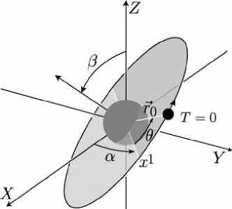
Figure 4: Satellite orbital parameters in the Sun-centered frame. For simplicity, the Earth is shown as if it were translated to the origin of the Sun-centered coordinates.

The oscillatory radial corrections $\delta r$ arising from the Lorentz-violating terms in Eq. (LABEL:esacc) take the generic form

$$\delta r=\sum_{n}[A_{n}\cos(\omega_{n}T+\phi_{n})+B_{n}\sin(\omega_{n}T+\phi_{n})].$$ (111)

The dominant amplitudes $A_{n}$ and $B_{n}$ and the values of the corresponding phases $\phi_{n}$ are listed in Table 2. The amplitudes are taken directly from Eqs. (310). The phases $\phi_{n}$ are related as indicated to the circular-orbit phase $\theta$ shown in Fig. 4.

Amplitude	Phase
$A_{2\omega}=-{{1}\over{12}}(\overline{s}^{11}-\overline{s}^{22})r_{0}$	$2\theta$
$B_{2\omega}=-{{1}\over{6}}\overline{s}^{12}r_{0}$	$2\theta$
$A_{2\omega-\omega_{0}}=-\omega er_{0}(\overline{s}^{11}-\overline{s}^{22})/16(\omega-\omega_{0})$	$2\theta$
$B_{2\omega-\omega_{0}}=-\omega er_{0}\overline{s}^{12}/8(\omega-\omega_{0})$	$2\theta$
$A_{\omega}=-\omega(\delta m)v_{0}r_{0}\overline{s}^{02}/M(\omega-\omega_{0})$	$\theta$
$B_{\omega}=\omega(\delta m)v_{0}r_{0}\overline{s}^{01}/M(\omega-\omega_{0})$	$\theta$
$A_{\Omega_{\oplus}}=V_{\oplus}r_{0}(b_{1}/b_{2})\overline{s}_{\Omega_{\oplus}c}$	$0$
$B_{\Omega_{\oplus}}=V_{\oplus}r_{0}(b_{1}/b_{2})\overline{s}_{\Omega_{\oplus}s}$	$0$

Table 2. Dominant Earth-satellite range oscillations.

The mass, position, frequency, and velocity variables appearing in Table 2 are defined in Table 1. The eccentricity of the orbit is denoted $e$, and for the analysis it is assumed to be much less than unity. The quantities $b_{1}$ and $b_{2}$ are defined in Eq. (269) of Appendix A. The anomalistic frequency $\omega_{0}$ is the frequency of the natural eccentric oscillations. Note that $\omega_{0}$ differs from $\omega$ in the presence of perturbing bodies and quadrupole moments. In the lunar case, for example, $2\pi/(\omega_{0}-\omega)\approx 8.9$ years anomecc .

Some of the combinations of SME coefficients appearing in Table 2 are labeled with indices 1 and 2, which refer to projections on the orbital plane. The label 1 represents projection onto the line of ascending nodes, while the label 2 represents projection onto the perpendicular direction in the orbital plane. Explicitly, the combinations are given in terms of the basic Sun-centered coefficients for Lorentz violation as

$$\overline{s}^{11}-\overline{s}^{22} = (\cos^{2}\alpha-\sin^{2}\alpha\cos^{2}\beta)\,\overline{s}^{XX}$$

$$+(\sin^{2}\alpha-\cos^{2}\alpha\cos^{2}\beta)\,\overline{s}^{YY}-\sin^{2}\beta\,\overline{s}^{ZZ}$$

$$+2\sin\alpha\cos\alpha(1+\cos^{2}\beta)\,\overline{s}^{XY}$$

$$+2\sin\beta\cos\beta\sin\alpha\,\overline{s}^{XZ}$$

$$-2\sin\beta\cos\beta\cos\alpha\,\overline{s}^{YZ},$$

$$\overline{s}^{12} = -\sin\alpha\cos\alpha\cos\beta\,\overline{s}^{XX}$$

$$+\cos\alpha\sin\alpha\cos\beta\,\overline{s}^{YY}$$

$$+(\cos^{2}\alpha-\sin^{2}\alpha)\cos\beta\,\overline{s}^{XY}$$

$$+\cos\alpha\sin\beta\,\overline{s}^{XZ}+\sin\alpha\sin\beta\,\overline{s}^{YZ},$$

$$\overline{s}^{01} = \cos\alpha\,\overline{s}^{TX}+\sin\alpha\,\overline{s}^{TY},$$

$$\overline{s}^{02} = -\sin\alpha\cos\beta\,\overline{s}^{TX}+\cos\alpha\cos\beta\,\overline{s}^{TY}$$ (112)

$$+\sin\beta\,\overline{s}^{TZ}.$$

Different combinations of coefficients for Lorentz violation also appear in Table 2, associated with the amplitudes of the oscillations at frequency $\Omega_{\oplus}$. The relevant combinations of these coefficients in the Sun-centered frame are explicitly given by

$$\overline{s}_{\Omega_{\oplus}c} = {\textstyle{{1}\over{2}}}(\sin\alpha\sin\eta\sin\beta\cos\beta$$

$$\qquad+\sin\alpha\cos\alpha\cos\eta\cos^{2}\beta$$

$$\qquad-\sin\alpha\cos\eta\cos\alpha)\overline{s}^{TX}$$

$$-(3\cos\eta+{\textstyle{{1}\over{2}}}\cos\eta\sin^{2}\alpha$$

$$\qquad+{\textstyle{{1}\over{2}}}\cos\alpha\sin\eta\sin\beta\cos\beta$$

$$\qquad+{\textstyle{{1}\over{2}}}\cos\eta\cos^{2}\alpha\cos^{2}\beta)\overline{s}^{TY}$$

$$-(3\sin\eta+{\textstyle{{1}\over{2}}}\cos\alpha\cos\eta\sin\beta\cos\beta$$

$$\qquad+{\textstyle{{1}\over{2}}}\sin^{2}\beta\sin\eta)\overline{s}^{TZ},$$

$$\overline{s}_{\Omega_{\oplus}s} = -(3+{\textstyle{{1}\over{2}}}\sin^{2}\alpha\cos^{2}\beta+{\textstyle{{1}\over{2}}}\cos^{2}\alpha)\overline{s}^{TX}$$ (113)

$$\qquad-{\textstyle{{1}\over{2}}}\cos\alpha\sin\alpha\sin^{2}\beta\overline{s}^{TY}$$

$$\qquad+{\textstyle{{1}\over{2}}}\sin\alpha\sin\beta\cos\beta\overline{s}^{TZ}.$$

V.2.3 Experiment

A feature of particular potential interest for experiments is the dependence of the coefficients in Table 2 on the orientation of the orbital plane. To illustrate this, consider first an equatorial satellite, for which $\beta=0$. The observable combinations of coefficients for Lorentz violation then reduce to

$$\overline{s}^{11}-\overline{s}^{22} = \cos 2\alpha(\overline{s}^{XX}-\overline{s}^{YY})+2\sin 2\alpha\,\overline{s}^{XY},$$

$$\overline{s}^{12} = -{\textstyle{{1}\over{2}}}\sin 2\alpha(\overline{s}^{XX}-\overline{s}^{YY})$$ (114)

$$+\cos 2\alpha\,\overline{s}^{XY}.$$

This implies that the $2\omega$ and $2\omega-\omega_{0}$ frequency bands of this orbit have sensitivity to the coefficients $\overline{s}^{XX}$, $\overline{s}^{YY}$, and $\overline{s}^{XY}$. If instead a polar satellite is considered, for which $\beta=\pi/2$, the same frequency bands have sensitivity to all six coefficients in $\overline{s}^{JK}$:

$$\overline{s}^{11}-\overline{s}^{22} = {\textstyle{{1}\over{2}}}(\overline{s}^{XX}+\overline{s}^{YY})+{\textstyle{{1}\over{2}}}\cos 2\alpha(\overline{s}^{XX}-\overline{s}^{YY})$$

$$+\sin 2\alpha\,\overline{s}^{XY}-\overline{s}^{ZZ},$$

$$\overline{s}^{12} = \cos\alpha\,\overline{s}^{XZ}+\sin\alpha\,\overline{s}^{YZ}.$$ (115)

These examples show that satellites with different orbits can place independent bounds on coefficients for Lorentz violation. A similar line of reasoning shows sensitivity to the $\overline{s}^{TJ}$ coefficients can be acquired as well.

For lunar laser ranging, the even-parity coefficients $\overline{s}^{JK}$ can be extracted from Eqs. (112) using the appropriate values of the longitude of the node and the inclination. For definiteness and to acquire insight, we adopt the values $\alpha\approx 125^{\circ}$ and $\beta\approx 23.5^{\circ}$. However, these angles vary for the Moon due to comparatively large newtonian perturbations, so some caution is needed in using the equations that follow. In any case, with these values we find the even-parity coefficients are given by

$$(\overline{s}^{11}-\overline{s}^{22})_{\leftmoon} = 0.08(\overline{s}^{XX}+\overline{s}^{YY}-2\overline{s}^{ZZ})$$

$$-0.31(\overline{s}^{XX}-\overline{s}^{YY})-1.7\overline{s}^{XY}$$

$$+0.60\overline{s}^{XZ}+0.42\overline{s}^{YZ},$$

$$(\overline{s}^{12})_{\leftmoon} = 0.43(\overline{s}^{XX}-\overline{s}^{YY})-0.31\overline{s}^{XY}$$ (116)

$$-0.23\overline{s}^{XZ}-0.33\overline{s}^{YZ}.$$

Evidently, lunar laser ranging measures two independent combinations of the $\overline{s}^{JK}$ coefficients.

For the odd-parity coefficients $\overline{s}^{TJ}$, adopting the same values for $\alpha$ and $\beta$ shows that lunar laser ranging offers sensitivity to the combinations

$$(\overline{s}^{01})_{\leftmoon} = -0.60\overline{s}^{TX}+0.82\overline{s}^{TY},$$

$$(\overline{s}^{02})_{\leftmoon} = -0.53\overline{s}^{TY}-0.75\overline{s}^{TX}+0.40\overline{s}^{TZ},$$

$$(\overline{s}_{\Omega_{\oplus}c})_{\leftmoon} = -3.1\overline{s}^{TY}-1.1\overline{s}^{TZ}+0.094\overline{s}^{TX},$$

$$(\overline{s}_{\Omega_{\oplus}s})_{\leftmoon} = -3.4\overline{s}^{TX}+0.037\overline{s}^{TY}+0.15\overline{s}^{TZ}.$$ (117)

This reveals that measuring the amplitudes at frequency $\omega$ and phase $\theta$ provides sensitivity to 2 combinations of the 3 independent coefficients $\overline{s}^{TJ}$. Provided one can also independently measure the amplitudes at frequency $\Omega$ and zero phase, the third independent coefficient in $\overline{s}^{TJ}$ can also be accessed.

Together the above considerations imply that lunar laser ranging can in principle measure at least 5 independent combinations of coefficients for Lorentz violation. In particular, the odd-parity coefficients $\overline{s}^{TJ}$ can be completely determined.

To estimate the experimental sensitivity attainable in lunar laser ranging, we assume ranging precision at the centimeter level, which has already been achieved onecm . With the standard lunar values $r_{0}=3.8\times 10^{8}$ m, $V_{\oplus}=1.0\times 10^{-4}$, $\omega/(\omega-\omega_{0})\approx 120$, and $e=0.055$, we find that lunar laser ranging can attain the following sensitivities: parts in $10^{11}$ on the coefficient $(\overline{s}^{12})_{\leftmoon}$, parts in $10^{10}$ on the combination $(\overline{s}^{11}-\overline{s}^{22})_{\leftmoon}$, and parts in $10^{7}$ on the coefficients $\overline{s}^{01}$, $\overline{s}^{02}$, $\overline{s}_{\Omega_{\oplus}s}$, $\overline{s}_{\Omega_{\oplus}c}$. These sensitivities may be substantially improved with the new Apache Point Observatory Lunar Laser-ranging Operation (APOLLO), which is currently under development in New Mexico with the goal of millimeter-ranging precision apollo .

Next, we consider ranging to artificial satellites. In practice, the realistic modeling of satellite orbits is more challenging than the Moon due to substantial perturbative effects. However, we show here that ranging to artificial satellites has the potential to be particularly useful for measuring independent combinations of the $\overline{s}^{JK}$ coefficients that are less readily accessible to lunar laser ranging due to the approximately fixed orientation of the plane of the lunar orbit.

The relevant coefficients for a generic satellite orbit are given in Eqs. (112) in terms of the right ascension $\alpha$ and inclination $\beta$. For the odd-parity coefficients, a similar argument applies as for the lunar case, so any one satellite can in principle measure all 3 coefficients $\overline{s}^{TJ}$. Using reasoning similar to that for lunar laser ranging, we find that any one satellite can make only two independent measurements of combinations of the even-parity coefficients $\overline{s}^{JK}$. It follows that any 2 satellites at different orientations can in principle measure 3 of the 4 combinations of components of $\overline{s}^{JK}$ to which lunar laser ranging is insensitive.

The reason that only 3 of the 4 can be measured is that the combination $\overline{s}^{XX}+\overline{s}^{YY}+\overline{s}^{ZZ}=\overline{s}^{TT}$ is absent from Eqs. (112) and hence only 5 combinations of the 6 coefficients in $\overline{s}^{JK}$ are measurable via the amplitudes in Table 2 for any set of orbit orientations. However, higher harmonics in $\omega$, $\Omega$, and other frequencies are likely to arise from the eccentric motion of the Moon or satellite. Although the corresponding amplitudes would be suppressed compared to those in Table 2, they could include terms from which the combination $\overline{s}^{XX}+\overline{s}^{YY}+\overline{s}^{ZZ}=\overline{s}^{TT}$ might be measured. The numerical code used to fit the data would include these amplitudes. Note that the strength of some signals might be enhanced by a suitable orientation of the satellite orbit, since the amplitudes in Table 2 depend on the orientation angles $\alpha$ and $\beta$ through the quantities $b_{1}$ and $b_{2}$ defined in Eq. (269).

Satellite	No.	$r_{0}$(m)	$\beta$	Ref.
ETALON	$2$	$2.5\times 10^{7}$	$65^{\circ}$	ilrs
GALILEO	$30$	$3.0\times 10^{7}$	$56^{\circ}$	galileo
GLONASS	$3$	$2.5\times 10^{7}$	$65^{\circ}$	ilrs
GPS	$2$	$2.6\times 10^{7}$	$55^{\circ}$	ilrs
LAGEOS I	$1$	$1.2\times 10^{7}$	$110^{\circ}$	ilrs
LAGEOS II	$1$	$1.2\times 10^{7}$	$53^{\circ}$	ilrs

Table 3. Some high-orbit satellites.

Some promising high-orbit satellite missions, both current and future, are listed in Table 3. Although beyond our present scope, it would be interesting to determine whether data from ranging to any of these satellites could be adapted to search for the signals in Table 2. As an estimate of attainable sensitivities, suppose centimeter-ranging sensitivity is feasible and take $r_{0}\approx 10^{7}$ m, $\omega/(\omega-\omega_{0})\approx 2\times 10^{3}$, and $e=0.010$. These values produce the following estimated sensitivities from laser ranging to artificial satellites: parts in $10^{9}$ on $\overline{s}^{11}-\overline{s}^{22}$, parts in $10^{10}$ on $\overline{s}^{12}$, parts in $10^{8}$ on $\overline{s}^{01}$, $\overline{s}^{02}$, and parts in $10^{5}$ on $\overline{s}_{\Omega_{\oplus}s}$, $\overline{s}_{\Omega_{\oplus}c}$.

Interesting possibilities may also exist for observing secular changes to the orbits of near-Earth satellites. Sensitivities comparable to some of those mentioned above may be attainable for certain coefficients nesat . A detailed analysis of this situation would require incorporating also contributions to the Earth-satellite acceleration $\alpha^{J}_{\rm ES}$ proportional to the spherical moment of inertia of the Earth. These contributions, which can arise from Lorentz-violating effects proportional to the potential $U^{JK}$ in Eq. (28), are small for high-orbit satellites or the Moon and so have been neglected in the analysis above, but they can be substantial for near-Earth orbits.

V.3 Laboratory experiments

This section considers some sensitive laboratory experiments on the Earth. Among ones already performed are gravimeter tests, analyzed in Refs. gcmw ; grvmet . For this case, the basic idea is to measure the force on a test mass held fixed above the Earth’s surface, seeking apparent variations in the locally measured value of Newton’s gravitational constant $G$. The coefficient space of the pure-gravity sector of the minimal SME to which this experiment is sensitive is explored below. Other sensitive existing laboratory experiments use various torsion pendula, with some already being applied to probe Lorentz violation in the fermion sector eexpt2 . This section also discusses some torsion-pendulum tests that could perform sensitive measurements of Lorentz symmetry in the gravitational sector.

V.3.1 Theory

To explore these ideas, we must first determine the dynamics of a test particle and establish the local acceleration at a point on the Earth’s surface in the presence of Lorentz violation controlled by the coefficients $\overline{s}^{\mu\nu}$. The results are required in a suitable observer coordinate system for experiments.

An observer on the surface of the Earth is accelerating and rotating with respect to the asymptotic inertial space. The appropriate coordinate system is therefore the proper reference frame of an accelerated and rotated observer nz ; mtw . At second order in the coordinate distance $x^{\hat{j}}$, the metric for this coordinate system can be written in the form

$$ds^{2} = -(dx^{\hat{0}})^{2}\big{[}1+2a^{\hat{j}}x^{\hat{j}}+(a^{\hat{j}}x^{\hat{j}})^{2}+(\omega^{\hat{j}}x^{\hat{j}})^{2}$$ (118)

$$-\omega^{2}x^{\hat{j}}x^{\hat{j}}+R_{\hat{0}\hat{j}\hat{0}\hat{k}}x^{\hat{j}}x^{\hat{k}}\big{]}$$

$$+2dx^{\hat{0}}dx^{\hat{j}}(\epsilon^{\hat{j}\hat{k}\hat{l}}\omega^{\hat{k}}x^{\hat{l}}-{\textstyle{{2}\over{3}}}R_{\hat{0}\hat{k}\hat{j}\hat{l}}x^{\hat{k}}x^{\hat{l}})$$

$$+dx^{\hat{j}}dx^{\hat{k}}(\delta_{\hat{j}\hat{k}}-{\textstyle{{1}\over{3}}}R_{\hat{j}\hat{l}\hat{k}\hat{m}}x^{\hat{l}}x^{\hat{m}}).$$

Here, we have introduced $x^{\hat{0}}$, which coincides along the worldline with the observer’s proper time.

From this metric, an effective Lagrange density can be established for test particle dynamics in the proper reference frame of an accelerated and rotated observer. The action for a test particle of mass $m$ takes the form

$$S = -m\int dx^{\hat{0}}\sqrt{{{-ds^{2}}\over{(dx^{\hat{0}})^{2}}}}$$ (119)

$$= \int dx^{\hat{0}}L.$$

For present purposes, it suffices to express the lagrangian as a post-newtonian series. Denote the coordinate position of the test particle by $x^{\hat{j}}$ and its coordinate velocity by $\dot{x}^{\hat{j}}$, where the dot signifies derivative with respect to $x^{\hat{0}}$. This velocity and the rotation velocity of the Earth’s surface are taken to be $O(1)$. The lagrangian then becomes

$$m^{-1}L = {\textstyle{{1}\over{2}}}(\dot{\vec{x}})^{2}-\vec{a}\cdot\vec{x}+{{1}\over{2}}(\vec{\omega}\times\vec{x})^{2}$$ (120)

$$+\dot{\vec{x}}\cdot(\vec{\omega}\times\vec{x})-{\textstyle{{1}\over{2}}}R_{\hat{0}\hat{j}\hat{0}\hat{k}}x^{\hat{j}}x^{\hat{k}}+\ldots.$$

In this expression, $\vec{a}$ is the observer acceleration, $\vec{\omega}$ is the observer angular velocity, and the various curvature components are taken to contain only the dominant contributions proportional to $\vec{\nabla}^{2}g_{00}$. The ellipses represent terms that contribute at $O(4)$ via post-newtonian quantities and sub-dominant curvature terms.

The dominant Lorentz-violating effects arise through $\vec{a}$. To establish the local acceleration in the proper reference frame in the presence of Lorentz violation, consider first the observer’s four acceleration in an arbitrary post-newtonian coordinate frame. This is given by the standard formula

$$a^{\mu}={{du^{\mu}}\over{d\tau}}+\Gamma^{\mu}_{\phantom{\mu}\nu\kappa}u^{\nu}u^{\kappa}.$$ (121)

We then choose the post-newtonian frame to be the Sun-centered frame described in Sec. V.1. In this frame, the spacetime metric is given by Eq. (94).

To express the local acceleration in the Sun-centered frame, the observer’s trajectory $x^{\Xi}$ is required. This can be adequately described to post-newtonian order by

$$x^{\Xi}=e^{\Xi}_{\phantom{\Xi}\tilde{k}}\xi^{\tilde{k}}+x^{\Xi}_{\oplus}.$$ (122)

In this equation, $x^{\Xi}_{\oplus}$ is the worldline of the Earth and $\xi^{\tilde{k}}$ is the spatial coordinate location of the observer in a frame centered on the Earth, for which indices are denoted with a tilde. The components of the comoving spatial basis in that frame are denoted $e^{\Xi}_{\phantom{\Xi}\tilde{k}}$. They can be obtained from Eq. (98) with $R^{jk}=0$ and the Earth velocity $v^{j}_{\oplus}$ given by Eq. (99) with $V^{J}=V^{J}_{\oplus}$. To sufficient post-newtonian accuracy, the observer’s coordinate location $\xi^{\tilde{k}}$ in the Earth frame can be taken as a vector pointing to the observer’s location and rotating with the Earth. Thus, modeling the Earth as a sphere of radius $R_{\oplus}$, we can write

$$\vec{\xi}=R_{\oplus}(\sin\chi\cos(\omega_{\oplus}T+\phi),\sin\chi\sin(\omega_{\oplus}T+\phi),\cos\chi),$$ (123)

where $\chi$ is the colatitude of the observer and $\phi$ is a standard phase fixing the time origin (see Ref. km , Appendix C): $\phi=\omega_{\oplus}(T_{\oplus}-T)$, where $T_{\oplus}$ is measured from one of the times when the $\hat{y}$ and $Y$ axis coincide.

To obtain explicitly the local acceleration, the potentials (28) must be evaluated for the Earth. They can be written as functions of the spatial position $\vec{X}$ in the Sun-centered frame, and the ones relevant here are given by

$$U = {{GM_{\oplus}}\over{|\vec{X}-\vec{x}_{\oplus}|}},$$

$$U^{JK} = {{GM_{\oplus}(X-x_{\oplus})^{J}(X-x_{\oplus})^{K}}\over{|\vec{X}-\vec{x}_{\oplus}|^{3}}}$$

$$-{{GI_{\oplus}}\over{3|\vec{X}-\vec{x}_{\oplus}|^{5}}}[3(X-x_{\oplus})^{J}(X-x_{\oplus})^{K}$$

$$\phantom{-{{GI_{\oplus}}\over{3|\vec{X}-\vec{x}_{\oplus}|^{5}}}}-\delta^{JK}|\vec{X}-\vec{x}_{\oplus}|^{2}],$$

$$V^{J} = {{GM_{\oplus}V^{J}_{\oplus}}\over{|\vec{X}-\vec{x}_{\oplus}|}}+\ldots.$$ (124)

In these equations, $M_{\oplus}$ is the mass of the Earth. The quantity $I_{\oplus}$ is the spherical moment of inertia of the Earth, given by the integral

$$I_{\oplus}=\int d^{3}y\rho(\vec{y})\vec{y}^{\hskip 2.0pt2}$$ (125)

over the volume of the Earth, where $\vec{y}$ is the vector distance from the center of the Earth and $\rho(\vec{y})$ is the density of the Earth. The ellipses in Eq. (124) represent neglected gravitomagnetic effects.

Inserting Eq. (122) into Eq. (121) yields the following components of the observer’s acceleration in the Sun-centered frame:

$$a^{T} = O(3),$$

$$a^{J} = g(1+{\textstyle{{3}\over{2}}}i_{1}\overline{s}^{TT}+{\textstyle{{3}\over{2}}}i_{2}\overline{s}^{KL}\delta^{K}_{\phantom{K}\tilde{k}}\delta^{L}_{\phantom{L}\tilde{l}}\hat{\xi}^{\tilde{k}}\hat{\xi}^{\tilde{l}})\delta^{J}_{\phantom{J}\tilde{j}}\hat{\xi}^{\tilde{j}}$$ (126)

$$\hskip-15.0pt-gi_{3}\overline{s}^{JK}\delta^{K}_{\phantom{K}\tilde{k}}\hat{\xi}^{\tilde{k}}+gi_{3}(\overline{s}^{TJ}V_{\oplus}^{K}\delta^{K}_{\phantom{K}\tilde{k}}\hat{\xi}^{\tilde{k}}+\overline{s}^{TK}V^{J}_{\oplus}\delta^{K}_{\phantom{K}\tilde{k}}\hat{\xi}^{\tilde{k}})$$

$$\hskip-15.0pt-3g(i_{1}\overline{s}^{TK}V_{\oplus}^{K}\delta^{J}_{\phantom{J}\tilde{j}}\hat{\xi}^{\tilde{j}}+i_{2}\overline{s}^{TK}V^{L}_{\oplus}\delta^{K}_{\phantom{K}\tilde{k}}\delta^{L}_{\phantom{L}\tilde{l}}\delta^{J}_{\phantom{J}\tilde{j}}\hat{\xi}^{\tilde{k}}\hat{\xi}^{\tilde{l}}\hat{\xi}^{\tilde{j}})$$

$$\hskip-15.0pt+\delta^{J}_{\phantom{J}\tilde{j}}d^{2}\xi^{\tilde{j}}/dT^{2}+O(4).$$

In these equations, the reference gravitational acceleration $g$ is

$$g=GM_{\oplus}/R^{2}_{\oplus},$$ (127)

and the quantities $i_{1}$, $i_{2}$, $i_{3}$ are defined by

$$i_{\oplus} = {{I_{\oplus}}\over{M_{\oplus}R^{2}_{\oplus}}},$$

$$i_{1} = 1+{\textstyle{{1}\over{3}}}i_{\oplus},$$

$$i_{2} = 1-{\textstyle{{5}\over{3}}}i_{\oplus},$$

$$i_{3} = 1-i_{\oplus}.$$ (128)

Note that the analysis here disregards possible tidal changes in the Earth’s shape and mass distribution mel ; cmw , which under some circumstances may enhance the observability of signals for Lorentz violation.

To obtain the corresponding expressions in the observer’s frame, it suffices to project Eq. (126) along the comoving basis vectors ${\bf e}_{\hat{\mu}}=e^{\Xi}_{\phantom{\Xi}\hat{\mu}}{\bf e}_{\Xi}$ of the accelerated and rotated observer on the Earth’s surface. Explicit expressions for these basis vectors are given by Eq. (98), with the observer velocity $v^{j}_{\rm o}$ and the rotation $R^{jk}$ taken as

$$v^{j}_{\rm o} = \delta_{J}^{\phantom{J}j}V^{J}_{\oplus}+\delta^{j}_{\phantom{j}\tilde{j}}d\xi^{\tilde{j}}/dT+O(3),$$

$$R^{jk} = R^{jk}_{Z}(\omega_{\oplus}T).$$ (129)

To sufficient approximation, we may use

$$\vec{V}_{\oplus}=V_{\oplus}(\sin\Omega_{\oplus}T,-\cos\eta\cos\Omega_{\oplus}T,-\sin\eta\cos\Omega_{\oplus}T),$$ (130)

where $V_{\oplus}$ is the mean Earth orbital speed and $\eta$ is the inclination of the Earth’s orbit, shown in Fig. 2.

We are free to use the observer rotational invariance of the metric (118) to choose the observer’s spatial coordinates $x^{\hat{j}}$ to coincide with the standard SME conventions for an Earth laboratory (see Ref. km , Appendix C). Thus, at a given point on the Earth’s surface, $\hat{z}$ points towards the zenith, $\hat{y}$ points east, and $\hat{x}$ points south. With these conventions, we find the desired expression for the local acceleration to be

$$a^{\hat{j}} = g(1+{\textstyle{{3}\over{2}}}i_{1}\overline{s}^{TT}+{\textstyle{{3}\over{2}}}i_{2}\overline{s}^{\hat{z}\hat{z}})\delta^{\hat{j}\hat{z}}-gi_{3}\overline{s}^{\hat{j}\hat{z}}$$ (131)

$$-\omega^{2}R_{\oplus}(\sin^{2}\chi\delta^{\hat{j}\hat{z}}+\sin\chi\cos\chi\delta^{\hat{j}\hat{x}})$$

$$+gi_{3}(\overline{s}^{T\hat{j}}V_{\oplus}^{\hat{z}}+\overline{s}^{T\hat{z}}V^{\hat{j}}_{\oplus})$$

$$-3g(i_{1}\overline{s}^{TJ}V_{\oplus}^{J}+i_{2}\overline{s}^{T\hat{z}}V^{\hat{z}}_{\oplus})\delta^{\hat{j}\hat{z}}+\ldots.$$

The ellipses represent newtonian tidal corrections from the Sun and Moon, along with $O(4)$ terms. The various projections of quantities along the local axes appearing in Eq. (131) are obtained using the comoving basis vectors ${\bf e}_{\hat{\mu}}=e^{\Xi}_{\phantom{\Xi}\hat{\mu}}{\bf e}_{\Xi}$. For example, $\overline{s}^{T\hat{j}}=e^{\phantom{\Xi}\hat{j}}_{\Xi}\overline{s}^{T\Xi}$. Typically, these projections introduce time dependence on $T$. Note, however, that the coefficient $\overline{s}^{TT}$ carries no time dependence up to $O(3)$ and hence represents an unobservable scaling.

V.3.2 Gravimeter tests

By restricting attention to motion along the $\hat{z}$ axis, the expression (131) for the local acceleration can be used to obtain the dominant Lorentz-violating contributions to the apparent local variation $\delta G$ of Newton’s gravitational constant, as would be measured with a gravimeter. This gives

$$a^{\hat{z}} = g(1+{\textstyle{{3}\over{2}}}i_{1}\overline{s}^{TT}+{\textstyle{{1}\over{2}}}i_{4}\overline{s}^{\hat{z}\hat{z}})-\omega^{2}R_{\oplus}\sin^{2}\chi$$ (132)

$$-gi_{4}\overline{s}^{T\hat{z}}V_{\oplus}^{\hat{z}}-3gi_{1}\overline{s}^{TJ}V_{\oplus}^{J},$$

where

$$i_{4} = 1-3i_{\oplus}.$$ (133)

The time dependence of the apparent variations in $G$ arises from the terms involving the indices $\hat{z}$ and the components $\overline{s}^{TJ}$. It can be decomposed in frequency according to

$${{\delta G}\over{G}} = \sum_{n}[C_{n}\cos(\omega_{n}T+\phi_{n})+D_{n}\sin(\omega_{n}T+\phi_{n})].$$

Explicit calculation of the time dependence using the comoving basis vectors yields the expressions for the amplitudes $C_{n}$, $D_{n}$ and phases $\phi_{n}$ listed in Table 3. In this table, the angle $\chi$ is the colatitude of the laboratory, and the other quantities are defined in the previous subsection.

Gravimeter Amplitudes
Amplitude	Phase
$C_{2\omega}={{1}\over{4}}i_{4}(\overline{s}^{XX}-\overline{s}^{YY})\sin^{2}\chi$	$2\phi$
$D_{2\omega}={{1}\over{2}}i_{4}\overline{s}^{XY}\sin^{2}\chi$	$2\phi$
$C_{\omega}={{1}\over{2}}i_{4}\overline{s}^{XZ}\sin 2\chi$	$\phi$
$D_{\omega}={{1}\over{2}}i_{4}\overline{s}^{YZ}\sin 2\chi$	$\phi$
$C_{2\omega+\Omega}=-{{1}\over{4}}i_{4}V_{\oplus}\overline{s}^{TY}(\cos\eta-1)\sin^{2}\chi$	$2\phi$
$D_{2\omega+\Omega}={{1}\over{4}}i_{4}V_{\oplus}\overline{s}^{TX}(\cos\eta-1)\sin^{2}\chi$	$2\phi$
$C_{2\omega-\Omega}=-{{1}\over{4}}i_{4}V_{\oplus}\overline{s}^{TY}(1+\cos\eta)\sin^{2}\chi$	$2\phi$
$D_{2\omega-\Omega}={{1}\over{4}}i_{4}V_{\oplus}\overline{s}^{TX}(1+\cos\eta)\sin^{2}\chi$	$2\phi$
$C_{\Omega}=V_{\oplus}[\overline{s}^{TY}\cos\eta({{1}\over{2}}i_{4}\sin^{2}\chi+3i_{1})+\overline{s}^{TZ}\sin\eta(3i_{1}+i_{4}\cos^{2}\chi)]$	$0$
$D_{\Omega}=-V_{\oplus}\overline{s}^{TX}({{1}\over{2}}i_{4}\sin^{2}\chi+3i_{1})$	$0$
$C_{\omega+\Omega}={{1}\over{4}}i_{4}V_{\oplus}\overline{s}^{TX}\sin 2\chi\sin\eta$	$\phi$
$D_{\omega+\Omega}=-{{1}\over{4}}i_{4}V_{\oplus}[\overline{s}^{TZ}(1-\cos\eta)-\overline{s}^{TY}\sin\eta]\sin 2\chi$	$\phi$
$C_{\omega-\Omega}={{1}\over{4}}i_{4}V_{\oplus}\overline{s}^{TX}\sin\eta\sin 2\chi$	$\phi$
$D_{\omega-\Omega}={{1}\over{4}}i_{4}V_{\oplus}[\overline{s}^{TZ}(1+\cos\eta)+\overline{s}^{TY}\sin\eta]\sin 2\chi$	$\phi$

Table 4. Gravimeter amplitudes.

Assuming each amplitude in Table 4 can be separately extracted from real data, it follows that gravimeter experiments can measure up to 4 independent coefficients in $\overline{s}^{JK}$ and all 3 coefficients in $\overline{s}^{TJ}$. Moreover, gravimeter experiments have attained impressive accuracies grvmet that would translate into stringent sensitivities on the pure-gravity coefficients in the minimal SME. A crude estimate suggests that gravimeter experiments fitting data to Eq. (LABEL:delg) could achieve sensitivity to $\overline{s}^{JK}$ at parts in $10^{11}$ and to $\overline{s}^{TJ}$ at parts in $10^{7}$. Possible systematics that would require attention include tidal influences from the Sun and Moon. These can, for example, generate oscillations contributing to Eq. (LABEL:delg) at frequencies $2\omega_{\oplus}$ and $\omega_{\oplus}$.

V.3.3 Torsion-pendulum tests

A complementary class of laboratory tests could exploit the anisotropy of the locally measured acceleration in the horizontal directions instead of the vertical one. Explicitly, the accelerations in the $\hat{x}$ and $\hat{y}$ directions are given by

$$a^{\hat{x}} = -gi_{3}\overline{s}^{\hat{x}\hat{z}}-\omega^{2}R_{\oplus}\sin\chi\cos\chi$$

$$+gi_{3}\overline{s}^{T\hat{z}}V_{\oplus}^{\hat{x}}+gi_{3}\overline{s}^{T\hat{x}}V^{\hat{z}}_{\oplus},$$

$$a^{\hat{y}} = -gi_{3}\overline{s}^{\hat{y}\hat{z}}+gi_{3}\overline{s}^{T\hat{z}}V^{\hat{y}}_{\oplus}+gi_{3}\overline{s}^{T\hat{y}}V^{\hat{z}}_{\oplus}$$ (135)

to order $O(3)$. In effect, the Lorentz-violating contributions to these expressions represent slowly varying accelerations in the horizontal directions as the Earth rotates and orbits the Sun. In contrast, the conventional centrifugal term in Eq. (135) is constant in time.

To gain insight into the experimental possibilities for testing the effects contained in Eqs. (135), consider an idealized scenario with a disk of radius $R$ and mass $M$ suspended at its center and positioned to rotate freely about its center of symmetry in the $\hat{x}$-$\hat{y}$ plane. We suppose that $N$ spherical masses, each of mass $m_{j}$, $j=1,2,\ldots,N$, are attached rigidly to the disk at radius $r_{0}<R$ and initially located at angular position $\theta_{j}$ relative to the $\hat{x}$ axis. For convenience, we write the masses as $m_{j}=\mu_{j}m$, where $m$ is a basic mass and $\mu_{j}$ are dimensionless numbers. In what follows, we assume a torsion suspension and focus attention on small angular deviations $\theta$ of the disk relative to its initial angular orientation. The apparatus with $N=3$ is depicted in Fig. 5. Note that the locations of the center of mass and the center of suspension are typically different. In practice, the technical challenge of keeping the disk level might be overcome in several ways, perhaps involving rigid suspension or magnetic support, but this is a secondary issue in the present context and is disregarded here.

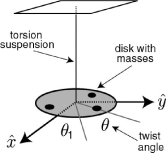
Figure 5: Idealized apparatus with $N=3$ masses.

Using Eq. (120), the effective potential energy for the apparatus can be constructed. Up to an overall constant, we find

$$V = -{\textstyle{{1}\over{2}}}mr_{0}[a^{\hat{x}}C_{N}+a^{\hat{y}}S_{N}+r_{0}\omega_{\oplus}^{2}\sin^{2}\chi(2C_{N}-1)]\theta^{2}$$ (136)

$$-mr_{0}(a^{\hat{x}}S_{N}-a^{\hat{y}}C_{N}+{\textstyle{{1}\over{2}}}a\omega_{\oplus}^{2}\sin^{2}\chi S_{N2})\theta.$$

In this expression, we have introduced the following quantities:

$$C_{N} = \sum_{j=1}^{N}\mu_{j}\cos\theta_{j},$$

$$S_{N} = \sum_{j=1}^{N}\mu_{j}\sin\theta_{j},$$

$$S_{N2} = \sum_{j=1}^{N}\mu_{j}\sin 2\theta_{j}.$$ (137)

These quantities depend on the number $N$ of masses used. Note that the effective potential (136) depends only on the distribution of the $N$ masses and is independent of the disk mass $M$.

The first part of Eq. (136) is proportional to $\theta^{2}$. This term contains contributions both from Lorentz violation and from the Earth’s rotation. It acts as an effective restoring force for the disk, producing a time-dependent shift to the effective spring constant of the system that primarily affects free oscillations. The second part of Eq. (136) is proportional to $\theta$, and it contains a time-independent contribution from the Earth’s rotation along with a Lorentz-violating piece. The latter produces a slowly varying Lorentz-violating torque $\tau=-dV/d\theta$ on the disk.

The oscillations of the system are determined by the second-order differential equation

$$I{{d^{2}\theta}\over{dT^{2}}}+2\gamma I{{d\theta}\over{dT}}+\kappa\theta=\tau,$$ (138)

where $I$ is the total moment of inertia of the disk and masses, and $\gamma$ is the damping parameter of the torsion fiber. In writing this equation, we have made use of the relation $d/dx^{\hat{0}}=(dT/dx^{\hat{0}})d/dT=(1+O(2))d/dT$.

The presence of the damping term in Eq. (138) ensures that free oscillations vanish in the steady-state solution. In the absence of additional torques, the steady-state solution is given by

$$\theta(T) = \sum_{n}{{i_{3}mr_{0}g}\over{I\sqrt{(\omega^{2}_{0}-\omega^{2}_{n})^{2}+4\gamma^{2}\omega^{2}_{n}}}}$$

$$\times\Big{(}[E_{n}\sin\alpha_{n}-F_{n}\cos\alpha_{n}]\sin(\omega_{n}T+\beta_{n})$$

$$-[E_{n}\cos\alpha_{n}+F_{n}\sin\alpha_{n}]\cos(\omega_{n}T+\beta_{n})\Big{)},$$

where

$$\beta_{n}=2\gamma\omega_{n}/(\omega^{2}_{n}-\omega^{2}_{0})$$ (140)

and, as before, $T$ is the time coordinate in the Sun-centered frame defined in Sec. V.1.1. Table 5 provides the amplitudes $E_{n}$, $F_{n}$ and the phases $\alpha_{n}$ in terms of quantities defined above.

Torsion-Pendulum Amplitudes
Amplitude	Phase
$E_{2\omega}=\overline{s}^{XY}C_{N}\sin\chi-{\textstyle{{1}\over{4}}}(\overline{s}^{XX}-\overline{s}^{YY})S_{N}\sin 2\chi$	$2\phi$
$F_{2\omega}=-{{1}\over{2}}(\overline{s}^{XX}-\overline{s}^{YY})C_{N}\sin\chi-{\textstyle{{1}\over{2}}}\overline{s}^{XY}S_{N}\sin 2\chi$	$2\phi$
$E_{\omega}=\overline{s}^{YZ}C_{N}\cos\chi-\overline{s}^{XZ}S_{N}\cos 2\chi$	$\phi$
$F_{\omega}=-\overline{s}^{XZ}C_{N}\cos\chi-\overline{s}^{ZY}S_{N}\cos 2\chi$	$\phi$
$E_{2\omega+\Omega}=-{\textstyle{{1}\over{2}}}V_{\oplus}\overline{s}^{TX}C_{N}(1-\cos\eta)\sin\chi-{\textstyle{{1}\over{4}}}V_{\oplus}\overline{s}^{TY}S_{N}(1-\cos\eta)\sin 2\chi$	$2\phi$
$F_{2\omega+\Omega}=-{\textstyle{{1}\over{2}}}V_{\oplus}\overline{s}^{TY}C_{N}(1-\cos\eta)\sin\chi+{\textstyle{{1}\over{4}}}V_{\oplus}\overline{s}^{TX}S_{N}(1-\cos\eta)\sin 2\chi$	$2\phi$
$E_{2\omega-\Omega}={\textstyle{{1}\over{2}}}V_{\oplus}\overline{s}^{TX}C_{N}(1+\cos\eta)\sin\chi+{\textstyle{{1}\over{4}}}V_{\oplus}\overline{s}^{TY}S_{N}(1+\cos\eta)\sin 2\chi$	$2\phi$
$F_{2\omega-\Omega}={\textstyle{{1}\over{2}}}V_{\oplus}\overline{s}^{TY}C_{N}(1+\cos\eta)\sin\chi-{\textstyle{{1}\over{4}}}V_{\oplus}\overline{s}^{TX}S_{N}(1+\cos\eta)\sin 2\chi$	$2\phi$
$E_{\omega+\Omega}={\textstyle{{1}\over{2}}}V_{\oplus}\overline{s}^{TY}C_{N}\sin\eta\cos\chi+V_{\oplus}\overline{s}^{TX}S_{N}\sin\eta({\textstyle{{1}\over{2}}}-\cos^{2}\chi)$	$\phi$
$\phantom{E_{\omega+\Omega}=\quad}+{\textstyle{{1}\over{2}}}V_{\oplus}\overline{s}^{TZ}C_{N}(\cos\eta-1)\cos\chi$
$F_{\omega+\Omega}=-{\textstyle{{1}\over{2}}}V_{\oplus}\overline{s}^{TX}C_{N}\sin\eta\cos\chi-V_{\oplus}\overline{s}^{TZ}S_{N}(1-\cos\eta)({\textstyle{{1}\over{2}}}-\cos^{2}\chi)$	$\phi$
$\phantom{F_{\omega+\Omega}=\quad}+V_{\oplus}\overline{s}^{TY}S_{N}\sin\eta({\textstyle{{1}\over{2}}}-\cos^{2}\chi)$
$E_{\omega-\Omega}={\textstyle{{1}\over{2}}}V_{\oplus}\overline{s}^{TZ}C_{N}(1+\cos\eta)\cos\chi+{\textstyle{{1}\over{2}}}V_{\oplus}\overline{s}^{TY}C_{N}\sin\eta\cos\chi$	$\phi$
$\phantom{E_{\omega-\Omega}=\quad}+V_{\oplus}\overline{s}^{TX}S_{N}\sin\eta({\textstyle{{1}\over{2}}}-\cos^{2}\chi)$
$F_{\omega-\Omega}=-{\textstyle{{1}\over{2}}}V_{\oplus}\overline{s}^{TX}C_{N}\sin\eta\cos\chi+V_{\oplus}\overline{s}^{TY}S_{N}\sin\eta({\textstyle{{1}\over{2}}}-\cos^{2}\chi)$	$\phi$
$\phantom{F_{\omega-\Omega}=\quad}+V_{\oplus}\overline{s}^{TZ}S_{N}(1+\cos\eta)({\textstyle{{1}\over{2}}}-\cos^{2}\chi)$
$E_{\Omega}=-{\textstyle{{1}\over{2}}}V_{\oplus}\overline{s}^{TY}S_{N}\cos\eta\sin 2\chi+V_{\oplus}\overline{s}^{TZ}S_{N}\sin\eta\sin 2\chi$	$0$
$F_{\Omega}={\textstyle{{1}\over{2}}}V_{\oplus}\overline{s}^{TX}S_{N}\sin 2\chi$	$0$

Table 5. Torsion-pendulum amplitudes.

To estimate the attainable sensitivities to Lorentz violation, we suppose the angular deflection of the apparatus can be measured at the nrad level, which in a different context has already been achieved with a torsion pendulum isql . For definiteness, we suppose that the disk radius is $R=10$ cm and that the $N=3$ masses have equal magnitude $m_{j}=M$ and are located at radius $r_{0}\approx R$ at angular locations $\theta_{1}=\pi/2$, $\theta_{2}=4\pi/3$, $\theta_{3}=5\pi/3$. Assuming a natural oscillation frequency $\omega_{0}\approx 10^{-2}$ Hz and a small damping parameter $\gamma\approx 10^{-3}$, and taking $i_{3}=2/5$ and $m\approx M$, we find the apparatus could attain sensitivity to the coefficients $\overline{s}^{JK}$ at the level of parts in $10^{15}$ and to the $\overline{s}^{TJ}$ coefficients at parts in $10^{11}$. These are idealized sensitivities, which are unlikely to be achieved in practice. Nonetheless, the result is of interest because it is about four orders of magnitude better than the (realistic) sensitivities that could be attained using current data from lunar laser ranging.

Provided the amplitudes in Table 5 can be separately extracted, and assuming measurements can be made with two different initial orientations $\theta_{1}$, it follows that these types of torsion-pendulum experiments can measure 4 coefficients in $\overline{s}^{JK}$ and all 3 independent coefficients in $\overline{s}^{TJ}$. As before, major systematics may include solar and lunar tidal effects.

Modifications of the apparatus proposed above could lead to improved sensitivities. One theoretically simple possibility is to decrease the effective spring constant of the system. Different kinds of pendulum could also be used. For example, the ring of point masses around the disk could be replaced with a ring of holes instead. A more radical possibility is to change the geometry of the apparatus. For example, one could replace the disk and masses with a thin rod lying in the horizontal plane and hanging from a torsion fiber. If the rod is suspended off center by some means while able to rotate freely about the vertical axis of the fiber, the steady-state oscillations again depend on the coefficients for Lorentz violation. In fact, the explicit results for this scenario can be obtained from Eq. (LABEL:th) and Table 5 by making the following replacements:

$$r_{0} \rightarrow {\textstyle{1\over 2}}(L-2d),$$

$$C_{N} \rightarrow \cos\theta_{0},$$

$$S_{N} \rightarrow \sin\theta_{0}.$$ (141)

Here, $L$ is the total length of the rod, and $d$ is the distance from the end of the rod to the point of suspension. Other quantities still appear but are reinterpreted: $m$ is the mass of the rod, $I$ is its moment of inertia, and $\theta_{0}$ is the initial angle the rod subtends to the $\hat{x}$ axis. Again, the practical issue of suspending a rod off center could conceivably be addressed with a rigid support system or magnetic levitation. The former method might allow an increase in sensitivity by reducing the effective torsion fiber frequency $\omega_{0}$ of the system. In any case, it would be of definite interest to investigate various experiments of this type.

Another potentially important issue is whether any of the existing torsion-pendulum experiments have sensitivity to Lorentz-violating effects. Consider, for example, an experiment designed to search for deviations from Newton’s law of gravity at sub-millimeter distances isql . The basic component of this experiment is a pair of disks positioned one above the other and with symmetric rings of holes in each. The upper disk is suspended as a torsion pendulum, in a manner analogous to that depicted in Fig. 5, while the lower one rotates uniformly. A key effect of the holes is to produce a time-varying torque on the pendulum that varies with the vertical separation between the two disks. Measurements of the torques at the rotation frequency and its harmonics offers high sensitivity to short-distance deviations from Newton’s law of gravity. The question of interest here is whether the presence of Lorentz violation would change the predicted newtonian torque in an observable way. A detailed analysis of this experiment is involved and lies beyond our present scope. However, some insight can be gained by using a simplified model that treats the rings of holes as two rings of point masses and comparable radii positioned one above the other, with the lower ring rotating.

Consider first the case of two point masses $m_{1}$ and $m_{2}$ at coordinate locations $\vec{x}_{1}$ and $\vec{x}_{2}$. The modified newtonian potential $V$ predicted by the pure-gravity sector of the minimal SME is

$$V=-{{Gm_{1}m_{2}}\over{|\vec{x}_{1}-\vec{x}_{2}|}}(1+{\textstyle{{1}\over{2}}}\hat{x}^{\hat{j}}\hat{x}^{\hat{k}}\overline{s}^{\hat{j}\hat{k}}),$$ (142)

where $\hat{x}=(\vec{x}_{1}-\vec{x}_{2})/|\vec{x}_{1}-\vec{x}_{2}|$. The non-newtonian effects are controlled by the SME coefficients for Lorentz violation $\overline{s}^{\hat{j}\hat{k}}$. Although Eq. (142) maintains the inverse-distance behavior of the usual newtonian potential, the associated force is misaligned relative to the vector $\hat{x}$ between the two point masses. It is therefore conceivable that an unconventional vertical dependence of the torque might arise in the experiment discussed above. To investigate this rigorously, the result (142) would be inserted into the computer code that models the experiment and determines the predicted torque isql .

In the context of the simplified model involving two rings of point masses, the difference between the newtonian and Lorentz-violating torques can be explored assuming a single nonzero coefficient $\overline{s}^{\hat{j}\hat{k}}$ in Eq. (142). We examined the Fourier components of the time-varying torque on the upper disk at harmonics of the rotational frequency of the bottom disk. The amplitudes of these Fourier components depend sensitively on the number of masses used, on the geometry of the experiment, and on the particular harmonic considered. This indicates that a careful analysis involving a detailed model of the actual experiment is necessary for definitive predictions. However, the results suggest that Lorentz-violating effects from certain coefficients $\overline{s}^{\hat{j}\hat{k}}$ of order $10^{-3}$ to $10^{-5}$ could be discernable at a separation of about 100 microns in experiments of this type, at the currently attainable torque sensitivities of about $10^{-17}$ Nm. Other experiments studying deviations from short-range newtonian gravity jl ; sjs may also be sensitive to these types of effects.

V.4 Gyroscope Experiment

In curved spacetime, the spin of a freely falling test body typically precesses relative to asymptotically flat spacetime lis ; lehspace . The primary relativistic effects for a gyroscope orbiting the Earth are the geodetic or de Sitter precession about an axis perpendicular to the orbit and the gravitomagnetic frame-dragging or Lens-Thirring precession about the spin axis of the Earth. In the present context of the post-newtonian metric for the pure-gravity sector of the minimal SME given in Eqs. (LABEL:g00)-(LABEL:gjk), we find that precession also occurs due to Lorentz violation. In particular, there can be precession of the spin axis about a direction perpendicular to both the spin axis of the Earth and the angular-momentum axis of the orbit.

V.4.1 Theory

To describe the motion of an orbiting gyroscope, we adopt standard assumptions mtw and use the Fermi-Walker transport equation given in coordinate-independent form by

$${\bf\nabla}_{\bf u}{\bf S}={\bf u}({\bf a}\cdot{\bf S}),$$ (143)

where ${\bf u}$ is the four-velocity of the gyroscope, ${\bf S}$ is the spin four-vector and ${\bf a}$ is the four-acceleration. The dot denotes the inner product with the metric two-tensor ${\bf g}$.

To obtain the equation of motion for the spin vector ${\bf S}$, we first construct a local frame ${\bf e}_{\hat{\mu}}$ that is comoving with ${\bf S}$ but is nonrotating with respect to the fixed stars in the asymptotically flat spacetime. The construction of this frame proceeds as in Sec. V.1, using the post-newtonian metric in Eqs. (94). The basis can be taken from Eq. (98) by setting the rotation terms to zero. Using Eq. (143), we can then find the proper-time derivative of ${\bf S}\cdot{\bf e}_{\hat{j}}$. It is given by

$${{d{\bf S}\cdot{\bf e}_{\hat{j}}}\over{d\tau}}={\bf S}\cdot({\bf\nabla}_{\bf u}{\bf e}_{\hat{j}}).$$ (144)

This represents the proper time rate of change of the spatial spin vector as measured in a comoving but nonrotating frame.

To display the dependence of the spin precession on the underlying geometry, which includes Lorentz-violating terms in the metric, the right-hand side of Eq. (144) can be expressed in the Sun-centered frame. This requires expressing the components of ${\bf S}$ and ${\bf\nabla}_{\bf u}{\bf e}_{\hat{j}}$ to the appropriate post-newtonian order. Of particular use for this purpose are the Sun-centered frame components of ${\bf e}_{\hat{j}}$, which are given by

$$e^{T}_{\phantom{T}\hat{j}} = \delta^{J}_{\phantom{J}\hat{j}}[v^{J}(1+h_{TT}+{\textstyle{{1}\over{2}}}v^{2})$$

$$\phantom{\delta^{\hat{j}J}}+{\textstyle{{1}\over{2}}}h_{JK}v^{K}+h_{TJ}]+O(4),$$

$$e^{J}_{\phantom{J}\hat{j}} = \delta^{K}_{\phantom{K}\hat{j}}[\delta_{JK}-{\textstyle{{1}\over{2}}}h_{JK}+{\textstyle{{1}\over{2}}}v^{J}v^{K}]+O(4).$$ (145)

We can then establish that

$${\bf S}^{T} = v^{J}S^{J}+O(2),$$

$${\bf S}^{J} = \delta^{J}_{\phantom{J}\hat{j}}S^{\hat{j}}+O(2),$$

$$({\bf\nabla}_{\bf u}{\bf e}_{\hat{j}})^{T} = \delta^{J}_{\phantom{J}\hat{j}}a^{J}+O(3),$$

$$({\bf\nabla}_{\bf u}{\bf e}_{\hat{j}})^{K} = \delta^{J}_{\phantom{J}\hat{j}}[{\textstyle{{1}\over{4}}}v^{K}\partial_{J}h_{TT}-{\textstyle{{1}\over{4}}}v^{J}\partial_{K}h_{TT}+a^{(J}v^{K)}$$ (146)

$$+\partial_{[J}h_{K]T}+v^{L}\partial_{[J}h_{K]L}]+O(4).$$

Combining Eqs. (145) and (146) via the expression

$${\bf S}\cdot({\bf\nabla}_{\bf u}{\bf e}_{\hat{j}})=S^{\Xi}({\bf\nabla}_{\bf u}{\bf e}_{\hat{j}})^{\Pi}g_{\Xi\Pi}$$ (147)

yields the general expression for the rate of change of the spatial spin vector of a gyroscope, valid to post-newtonian $O(3)$. It is given by

$${{dS_{\hat{j}}}\over{d\tau}} = S^{\hat{k}}\delta^{K}_{\phantom{K}\hat{k}}\delta^{J}_{\phantom{J}\hat{j}}\big{(}v^{[J}a^{K]}+{\textstyle{{1}\over{4}}}v^{K}\partial_{J}h_{TT}-{\textstyle{{1}\over{4}}}v^{J}\partial_{K}h_{TT}$$ (148)

$$\phantom{S^{\hat{k}}\delta^{\hat{k}K}\delta^{\hat{j}J}}+\partial_{[J}h_{K]T}+v^{L}\partial_{[J}h_{K]L}\big{)}.$$

In the limit of the usual general-relativistic metric, this agrees with existing results cmw ; mtw .

V.4.2 Gyroscope in Earth orbit

In this subsection, we specialize to a gyroscope in a near-circular orbit around the Earth. For this case, the acceleration term vanishes.

The first step is to determine the contributions to the metric potentials (28) from the various relevant bodies in the solar system. For simplicity, we focus on the potentials due to the Earth, neglecting any contributions from the Sun, Moon, or other sources, and we take the Earth as a perfect sphere rotating uniformly at frequency $\omega$ and with spherical moment of inertia $I_{\oplus}$ give by Eq. (125). For convenience in what follows, we introduce a quantity ${\tilde{i}}_{\oplus}$ related to $I_{\oplus}$ along with corresponding quantities ${\tilde{i}}_{(\alpha)}$ defined for any real number $\alpha$ by the equations

$${\tilde{i}}_{\oplus} = {{I_{\oplus}}\over{M_{\oplus}r^{2}_{0}}},$$

$${\tilde{i}}_{(\alpha)} = 1+\alpha{\tilde{i}}_{\oplus},$$ (149)

where $r_{0}$ is the mean orbital distance to the gyroscope.

The explicit form is required for five of the six types of metric potentials in Eq. (28). Some general-relativistic contributions from the potential $W^{J}$ involving the Earth’s angular momentum $J^{K}_{\oplus}=2I_{\oplus}\omega^{K}/3$ can be converted into ones involving $V^{J}$ by using the identity (30). Also, contributions from the potential $Y^{JKL}$ can be converted into ones involving only the other potentials by virtue of the antisymmetrization in Eq. (148) and the identity (LABEL:chijident). The five necessary Earth potentials can be written as functions of the spatial position $\vec{X}$ in the Sun-centered frame, given by

$$U = {{GM_{\oplus}}\over{|\vec{X}-\vec{R}|}},$$

$$U^{JK} = {{GM_{\oplus}(X-R)^{J}(X-R)^{K}}\over{|\vec{X}-\vec{R}|^{3}}}$$

$$-{{GI_{\oplus}}\over{3|\vec{X}-\vec{R}|^{5}}}[3(X-R)^{J}(X-R)^{K}$$

$$\phantom{-{{GI_{\oplus}}\over{3|\vec{X}-\vec{R}|^{5}}}}-\delta^{JK}|\vec{X}-\vec{R}|^{2}],$$

$$V^{J} = {{GM_{\oplus}V^{J}_{\oplus}}\over{|\vec{X}-\vec{R}|}}+{{G\epsilon^{JKL}J^{K}_{\oplus}(X-R)^{L}}\over{2|\vec{X}-\vec{R}|^{3}}},$$

$$W^{J} = V_{\oplus}^{K}U^{KJ}+\ldots,$$

$$X^{JKL} = V_{\oplus}^{J}U^{KL}+\ldots,$$ (150)

where $\vec{R}=R\hat{R}$ is the Earth’s location in the Sun-centered frame and $V^{J}_{\oplus}$ is its velocity. Explicit expressions for these quantities are given in Eq. (LABEL:R) of Appendix A and in the associated discussion.

The ellipses in Eqs. (150) represent omitted pieces of the potentials arising from the purely rotational component of the Earth’s motion, which generate gravitomagnetic effects involving Lorentz violation. A crude estimate reveals that these gravitomagnetic terms are suppressed relative to the associated geodetic terms displayed in Eqs. (150) by about two orders of magnitude. As a result, although gravitomagnetic frame-dragging terms are crucial for tests of conventional general relativity mtw ; cmw , they can be neglected for studies of the dominant Lorentz-violating contributions to the spin precession. For simplicity, the frame-dragging precession effects involving Lorentz violation are omitted in what follows.

For use in Eq. (148), these potentials must be evaluated along the worldline of the gyroscope. At post-newtonian order, this worldline is adequately described by the expressions for an arbitrary satellite orbit given in Appendix A. Thus, the value of $(\vec{X}-\vec{R})$ along the worldline can be written as

$$(\vec{X}-\vec{R})_{\rm gyro}=r_{0}\hat{\rho},$$ (151)

where $\hat{\rho}$ is given by Eq. (210). To post-newtonian order, the gyroscope velocity $v^{J}_{\rm gyro}$ can be taken as $v^{J}_{\rm gyro}=V^{J}_{\oplus}+v^{J}_{0}$, where $v^{J}_{0}$ is the mean orbital velocity defined by $\vec{v}_{0}=d(r_{0}\hat{\rho})/dT=v_{0}\hat{\tau}$. The normal to the plane of the orbit is $\hat{\sigma}=\hat{\rho}\times\hat{\tau}$.

Inserting the potentials (150) into Eq. (148) and evaluating along the worldline yields a result that can be separated into two pieces,

$${{dS_{\hat{j}}}\over{d\tau}} = {{dS^{E}_{\hat{j}}}\over{d\tau}}+{{dS^{\overline{s}}_{\hat{j}}}\over{d\tau}}.$$ (152)

The first piece is the standard result from general relativity, given by

$${{dS^{E}_{\hat{j}}}\over{d\tau}} = g\delta^{J}_{\phantom{J}\hat{j}}S^{K}[(-3v^{[K}_{0}\hat{\rho}^{J]}+V^{[K}_{\oplus}\hat{\rho}^{J]})$$

$$\qquad-{{2J_{\oplus}^{L}}\over{M_{\oplus}r_{0}}}(\epsilon^{JKL}+3\epsilon^{LM[J}\hat{\rho}^{K]}\hat{\rho}^{M})],$$

where the reference gravitational acceleration $g$ is now

$$g=GM_{\oplus}/r^{2}_{0}.$$ (154)

The second piece is proportional to the coefficients for Lorentz violation $\overline{s}^{JK}$, and it takes the form

$${{dS^{\overline{s}}_{\hat{j}}}\over{d\tau}} = g\delta^{J}_{\phantom{J}\hat{j}}S^{K}\Big{[}2\overline{s}^{T[K}\hat{\rho}^{J]}+4{\tilde{i}}_{(-1)}\overline{s}^{L[J}v^{K]}_{0}\hat{\rho}^{L}$$

$$\hskip-5.0pt+v^{[K}_{0}\hat{\rho}^{J]}(-{\textstyle{{5}\over{2}}}{\tilde{i}}_{(3/5)}\overline{s}^{TT}-{\textstyle{{9}\over{2}}}{\tilde{i}}_{(-5/3)}\overline{s}^{LM}\hat{\rho}^{L}\hat{\rho}^{M})$$

$$\hskip-5.0pt+{\tilde{i}}_{(1)}\overline{s}^{L[K}\hat{\rho}^{J]}v^{L}_{0}-2\overline{s}^{L[K}\hat{\rho}^{J]}V^{L}_{\oplus}+{\tilde{i}}_{(-1)}\overline{s}^{L[K}V^{J]}_{\oplus}\hat{\rho}^{L}$$

$$\hskip-5.0pt+V^{[K}_{\oplus}\hat{\rho}^{J]}(-{\textstyle{{1}\over{2}}}\overline{s}^{TT}{\tilde{i}}_{(-1)}+{\textstyle{{3}\over{2}}}{\tilde{i}}_{(-5/3)}\overline{s}^{LM}\hat{\rho}^{L}\hat{\rho}^{M})\Big{]}.$$

Among the effects described by the result (152) are oscillations of the orientation of the gyroscope spin vector that occur at frequencies $\omega$, $\omega\pm\Omega_{\oplus}$, and higher harmonics. At the frequency $\omega$, these oscillations change the angular orientation of a gyroscope by roughly $\delta\theta\approx 2\pi v_{0}^{2}$. For a gyroscope in low Earth orbit, this is $\delta\theta\approx 8\times 10^{-4}$ arcseconds, well below observable levels for existing sensitivity to nonsecular changes.

We therefore focus instead on the dominant secular contributions to the motion of the gyroscope spin. Averaging various key quantities over an orbital period yields the following results:

$$<r^{J}_{0}r^{K}_{0}> = {\textstyle{1\over 2}}r_{0}^{2}(\delta^{JK}-\hat{\sigma}^{J}\hat{\sigma}^{K}),$$

$$<r^{J}_{0}v^{K}_{0}> = {\textstyle{1\over 2}}r_{0}v_{0}\epsilon^{JKL}\hat{\sigma}^{L},$$

$$<r^{K}_{0}r^{[L}_{0}v^{M]}_{0}r^{N}_{0}> = {\textstyle{{1}\over{4}}}r^{3}_{0}v_{0}\epsilon^{LMP}\hat{\sigma}^{P}(\delta^{KN}-\hat{\sigma}^{K}\hat{\sigma}^{N}),$$

$$<r^{J}_{0}r^{K}_{0}V_{\oplus}^{L}r^{M}_{0}> \approx 0,$$

$$<r^{J}_{0}V_{\oplus}^{K}> \approx 0,$$

$$<r^{J}_{0}> = 0.$$ (156)

In these equations, the vector $\hat{\sigma}^{J}$ is given explicitly as

$$\hat{\sigma}^{J} = (\sin\alpha\sin\beta,-\cos\alpha\sin\beta,\cos\beta),$$ (157)

where the angles $\alpha$ and $\beta$ are those defined in Sec. V.2 and Fig. 4. Note that the averaging process eliminates the terms involving $V^{J}_{\oplus}$. In the conventional case, such terms can be shown to be unobservable in principle by a consideration of the physical precession referenced to the fixed stars cmw ; cmwgyro . It is an open question whether this stronger result remains true in the presence of Lorentz violation.

Combining the above results yields the vector equation for the secular evolution of the gyroscope spin. It can be written in the form

$${{d\vec{S}}\over{dt}}=gv_{0}\vec{\Omega}\times\vec{S}.$$ (158)

The secular precession frequency $\vec{\Omega}$ is comprised of two pieces,

$$\Omega^{J} = \Omega^{J}_{E}+\Omega^{J}_{\overline{s}}.$$ (159)

The first term $\Omega^{J}_{E}$ contains precession due to conventional effects in general relativity, and it is given by

$$\Omega^{J}_{E} = {\textstyle{{3}\over{2}}}\hat{\sigma}^{J}+{{J_{\oplus}^{K}}\over{2M_{\oplus}r_{0}v_{0}}}(\delta^{JK}-3\hat{\sigma}^{J}\hat{\sigma}^{K}).$$ (160)

The second term $\Omega^{J}_{\overline{s}}$ contains contributions from the coefficients for Lorentz violation $\overline{s}^{JK}$, and it has the form

$$\Omega^{J}_{\overline{s}} = {\textstyle{{9}\over{8}}}({\tilde{i}}_{(-1/3)}\overline{s}^{TT}-{\tilde{i}}_{(-5/3)}\overline{s}^{KL}\hat{\sigma}^{K}\hat{\sigma}^{L})\hat{\sigma}^{J}$$ (161)

$$+{\textstyle{{5}\over{4}}}{\tilde{i}}_{(-3/5)}\overline{s}^{JK}\hat{\sigma}^{K}.$$

In the limit of no Lorentz violation, Eq. (159) reduces as expected to the conventional result (160) of general relativity involving the geodetic precession arising from the spacetime curvature near the Earth and the frame-dragging precession arising from the rotation of the Earth.

V.4.3 Gravity Probe B

Gravity Probe B (GPB) gpb is an orbiting-gyroscope experiment that has potential sensitivity to certain combinations of coefficients contained in Eq. (161). Our general results (158) for the spin precession can be specialized to this experiment. In terms of the angles in Fig. 4, the GPB orbit is polar with $\alpha=163^{\circ}$ and $\beta=90^{\circ}$. One consequence of the polar orbit is that the normal vector $\hat{\sigma}^{J}$ to the orbital plane appearing in Eq. (161) reduces to the simpler form

$$\hat{\sigma}^{J} = (\sin\alpha,-\cos\alpha,0).$$ (162)

The terms in Eq. (158) proportional to $\hat{\sigma}\times\vec{S}$ act to precess the gyroscope spin in the plane of the orbit. They include the geodetic precession in Eq. (160) predicted by general relativity, along with modifications due to Lorentz violation. The magnitude of the precession is determined by the projection $\hat{\sigma}\cdot\vec{\Omega}$. The explicit form of the relevant projection of $\vec{\Omega}$ arising due to Lorentz violation is found to be

$$\Omega^{\sigma}_{\overline{s}} = {\textstyle{{9}\over{8}}}{\tilde{i}}_{(-1/3)}\overline{s}^{TT}+{\textstyle{{1}\over{8}}}{\tilde{i}}_{(9)}\overline{s}^{JK}\hat{\sigma}^{J}\hat{\sigma}^{K}.$$ (163)

The terms in Eq. (158) proportional to $\hat{J}\times\vec{S}$, where $\vec{J}$ is the Earth’s angular momentum, cause precession of the gyroscope spin in the plane perpendicular to $\vec{J}$. Since $\vec{J}$ lies along $\hat{Z}$, this is the $XY$ plane of Fig. 4. These terms include the frame-dragging effect in Eq. (160) predicted by general relativity, together with effects due to Lorentz violation. These have magnitude determined by the projection $\hat{Z}\cdot\vec{\Omega}$. For the contributions due to Lorentz violation, we find the explicit form

$$\Omega^{Z}_{\overline{s}} = {\textstyle{{5}\over{4}}}{\tilde{i}}_{(-3/5)}\overline{s}^{ZK}\hat{\sigma}^{K}.$$ (164)

In addition to the above, however, Lorentz violation induces a third type of precession that is qualitatively different from those predicted by general relativity. This is a precession of the gyroscope spin in the plane with normal $\hat{n}$ along $\hat{\sigma}\times\hat{J}$. With the definitions shown in Fig. 4, this normal is given by $\hat{n}=(\cos\alpha,\sin\alpha,0)$. The magnitude of the associated precession is given by $\hat{n}\cdot\vec{\Omega}$. We obtain

$$\Omega^{n}_{\overline{s}} = {\textstyle{{5}\over{4}}}{\tilde{i}}_{(-3/5)}\overline{s}^{JK}\hat{n}^{J}\hat{\sigma}^{K}.$$ (165)

The GPB experiment is expected to attain sensitivity to secular angular precessions of the order of $5\times 10^{-4}$ arcseconds per year. If the spin precession in the three orthogonal directions can be disentangled, GPB could produce the first measurements of three combinations of the $\overline{s}^{JK}$ coefficients, including one involving precession about the $\hat{n}$ direction. The attainable sensitivity to $\overline{s}^{JK}$ coefficients is expected to be at the $10^{-4}$ level.

V.5 Binary pulsars

Binary pulsars form a useful testing ground for general relativity bp1 ; cmw01 . This subsection examines the possibility of probing SME coefficients for Lorentz violation using pulsar timing data gl2 . We find that Lorentz violation induces secular variations in the orbital elements of binary-pulsar systems, along with modifications to the standard pulsar timing formula. The discussion is separated into five parts: one establishing the basic framework and assumptions, a second presenting the secular changes, a third describing the timing formula, a fourth determining some experimental effects, and a final part explaining the transformation between the frame used to study the properties of the binary pulsar and the standard Sun-centered frame.

The reader is cautioned that the notation for the binary-pulsar systems in this subsection is chosen to match the literature and differs in certain respects from the notation adopted elsewhere in the paper. This notation is described in Sec. V.5.1.

V.5.1 Basics

The general problem of describing the dynamics of binary pulsars is complicated by the strong-field gravitational properties of the spacetime regions close to the pulsar and its companion. Nonetheless, provided the typical radius of the pulsar and companion are much smaller than the average orbital distance between them, the orbital dynamics can be modeled with an effective post-newtonian description.

One standard approach is to construct a modified Einstein-Infeld-Hoffman (EIH) lagrangian describing the post-newtonian dynamics of the system cmw . In principle, an analysis of the effects of Lorentz violation could be performed via a modified EIH approach based on the action of the pure-gravity sector of the minimal SME. This would involve generalizing Eq. (54) to allow for the usual EIH effects, along with modifications to the Lorentz-violating behavior arising from the structure of the pulsar and its companion. A detailed analysis along these lines would be of interest but lies beyond the scope of the present work.

In fact, a simpler approach suffices to extract key features arising from Lorentz violation. Instead of a full EIH-type treatment, we adopt in what follows a simplified picture and consider only the effects arising in a point-mass approximation for each of the two bodies in the system. To retain some generality and an EIH flavor in the treatment, we interpret the gravitational constant, the masses, and the coefficients for Lorentz violation as effective quantities bp3 . However, the results disregard details of possible strong-field gravitational effects or consequences of nonzero multipole moments and tidal forces across the pulsar and companion. The reader is cautioned that the corresponding conventional effects from newtonian theory can be crucial for studies of binary pulsars, so they should be included in a complete analysis. Nonetheless, the results obtained here offer a good baseline for the sensitivities to Lorentz violation that might be achieved through observations of binary pulsars.

The analysis that follows makes use of the standard keplerian characterization of an elliptical orbit bp2 . Some of the key quantities are displayed in Fig. 6. In this figure, the point P is the location of the pulsar at time $t$, and it lies a coordinate distance $r$ from the focus F of the elliptical orbit. The line segments CA and CB are the semimajor axes, each of length $a$. The eccentric anomaly $E$ is defined as the angle ACQ, where Q is the point on the enclosing circle with the same abcissa as P. The true anomaly $f$ is defined as the angle AFP, while $\omega$ is the angle subtended between the line of ascending nodes FN and the major axis of the ellipse.

The general solution of the elliptic two-body problem is given in terms of the time $t$ and six integration constants called the orbital elements. Three of the latter are associated with inherent properties of the ellipse: the semimajor axis length $a$, the eccentricity $e$, and a phase variable $l_{0}$ called the mean anomaly at the epoch. The other three describe the position of the ellipse in the reference coordinate system: the inclination $i$, the longitude of the ascending node $\Omega$, and the angle $\omega$ defined above. The orbital frequency is denoted $n$, and it is related as usual to the period $P_{b}=2\pi/n$. Standard expressions relate these various quantities. For example, the eccentric anomaly $E$ is related to the mean anomaly $l_{0}$ at the epoch $t=t_{0}$ by

$$E-e\sin E=l_{0}+n(t-t_{0}).$$ (166)

The reader is referred to Refs. bp2 for further details.

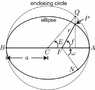
Figure 6: Definitions for the elliptical orbit.

V.5.2 Secular changes

We begin the analysis with the derivation of the secular changes in the orbital elements of a binary-pulsar system that arise from Lorentz violation. Adopting the point-mass limit as described above, Eq. (52) can be used to determine the relative coordinate acceleration of the pulsar and companion, which are taken to be located at $\vec{r}_{1}$ and $\vec{r}_{2}$, respectively. The result can be written in the form of Eq. (LABEL:esacc), with the quadrupole moment set to zero and the effects from external bodies omitted.

It is convenient for the analysis to choose a post-newtonian frame with origin at the center of mass of the binary-pulsar system. The newtonian definition of the center of mass suffices here because the analysis is perturbative. The frame is taken to be asymptotically inertial as usual, so that the coefficients for Lorentz violation obey Eqs. (11). The coordinates in this frame are denoted $x^{\mu}=(t,x^{j})$, and the corresponding basis is denoted ${\bf e}_{\mu}$. The issue of matching the results to the Sun-centered frame is addressed in Sec. V.5.5 below.

In this post-newtonian binary-pulsar frame, the relative acceleration of the pulsar and companion can be written

$${{d^{2}r^{j}}\over{dt^{2}}} = -{{GM}\over{r^{3}}}[(1+{\textstyle{{3}\over{2}}}\overline{s}^{00})r^{j}-\overline{s}^{jk}r^{k}+{\textstyle{{3}\over{2}}}\overline{s}^{kl}\hat{r}^{k}\hat{r}^{l}r^{j}]$$ (167)

$$+{{2G\delta m}\over{r^{3}}}[\overline{s}^{0k}v^{k}r^{j}-\overline{s}^{0j}v^{k}r^{k}]+\ldots,$$

where the definitions of $\vec{r}$, $r$, $\vec{v}$, $M$ and $\delta m$ parallel those adopted in Table 1 of Sec. V.2. The ellipses here represent corrections from multipole moments, from general relativistic effects at $O(4)$, and from Lorentz-violating effects at $O(4)$. Note that enhancements of secular effects stemming from general relativistic corrections at $O(4)$ are known to occur under some circumstances bp3 , but the issue of whether $O(4)$ enhancements can occur in the SME context is an open question lying beyond our present scope.

To establish the observational effects of Lorentz violation that are implied by Eq. (167), we adopt the method of osculating elements bp2 . This method assumes the relative motion of the binary pulsar and companion is instantaneously part of an ellipse. The subsequent motion is obtained by letting the orbital elements vary with time while keeping the equations of the ellipse fixed. In the present instance, the unperturbed ellipse solves the equation

$${{d^{2}r^{j}}\over{dt^{2}}}=-{{GM}\over{r^{3}}}(1+{\textstyle{{3}\over{2}}}\overline{s}^{00})r^{j}.$$ (168)

Note that this implies the frequency and the semimajor axis of the orbit are related by

$$n^{2}a^{3}=GM(1+{\textstyle{{3}\over{2}}}\overline{s}^{00}).$$ (169)

The remaining terms are then viewed as a perturbing acceleration $\alpha^{\prime j}$, given in this case by

$$\alpha^{\prime j} = {{GM}\over{r^{3}}}\overline{s}^{jk}r^{k}-{\textstyle{{3}\over{2}}}{{GM}\over{r^{3}}}\overline{s}^{kl}\hat{r}^{k}\hat{r}^{l}r^{j}$$ (170)

$$+{{2G\delta m}\over{r^{3}}}[\overline{s}^{0k}v^{k}r^{j}-\overline{s}^{0j}v^{k}r^{k}].$$

The idea is to extract from this equation the variations in the six orbital elements $a$, $e$, $l_{0}$, $i$, $\Omega$, $\omega$ describing the instantaneous ellipse for the relative motion.

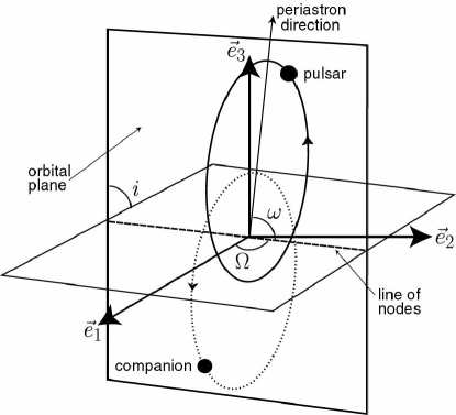
Figure 7: Elliptical orbits in the post-newtonian frame of the binary pulsar.

The elliptical orbits of the pulsar and companion, referred to the chosen post-newtonian frame, are illustrated in Fig. 7. The relative motion can also be represented by an ellipse in the same plane. To specify the orientation of the orbit, three linearly independent unit vectors are needed. A natural set includes one vector $\vec{k}$ normal to the orbital plane, a second vector $\vec{P}$ pointing from the focus to the periastron, and a third vector $\vec{Q}=\vec{k}\times\vec{P}$ perpendicular to the first two. This triad of vectors can be expressed in terms of the spatial basis ${\bf e}_{j}$ for the post-newtonian frame. Explicitly, these vectors are given by

$$\vec{P} = (\cos\Omega\cos\omega-\cos i\sin\Omega\sin\omega)\vec{e}_{1}$$

$$+(\sin\Omega\cos\omega+\cos i\cos\Omega\sin\omega)\vec{e}_{2}$$

$$+\sin i\sin\omega\vec{e}_{3},$$

$$\vec{Q} = -(\cos\Omega\sin\omega+\cos i\sin\Omega\cos\omega)\vec{e}_{1}$$

$$+(\cos i\cos\Omega\cos\omega-\sin\Omega\sin\omega)\vec{e}_{2}$$

$$+\sin i\cos\omega\vec{e}_{3},$$

$$\vec{k} = \sin i\sin\Omega\vec{e}_{1}-\sin i\cos\Omega\vec{e}_{2}$$ (171)

$$+\cos i\vec{e}_{3}.$$

In terms of these vectors, the unperturbed elliptical orbit can be expressed as

$$\vec{r} = {{a(1-e^{2})}\over{1+e\cos f}}(\vec{P}\cos f+\vec{Q}\sin f).$$ (172)

Following standard methods, we insert the solution $\vec{r}$ for the elliptic orbit given by Eq. (172) into the expression (170) for the perturbative acceleration, project the result as appropriate to extract the orbital elements, and average over one orbit. The averaging is performed via integration over the true anomaly $f$, which serves as the phase variable. Details of this general procedure are discussed in Refs. bp2 .

After some calculation, we find the secular evolutions of the semimajor axis and the eccentricity are given by

$$\langle{{da}\over{dt}}\rangle = 0,$$

$$\langle{{de}\over{dt}}\rangle = 2n(1-e^{2})^{1/2}\Big{[}{{(e^{2}-2\varepsilon)}\over{2e^{3}}}\overline{s}_{PQ}-{{\delta m}\over{M}}{{na\varepsilon}\over{e^{2}}}\overline{s}_{P}\Big{]},$$

where the eccentricity function $\varepsilon(e)$ is given by

$$\varepsilon(e) = 1-(1-e^{2})^{1/2}.$$ (174)

The secular evolutions of the three orbital elements associated with the orientation of the ellipse relative to the post-newtonian frame are

$$\langle{{d\omega}\over{dt}}\rangle = -{{n}\over{\tan i(1-e^{2})^{1/2}}}\Big{[}{{\varepsilon}\over{e^{2}}}\overline{s}_{kP}\sin\omega$$

$$\qquad+{{(e^{2}-\varepsilon)}\over{e^{2}}}\overline{s}_{kQ}\cos\omega-{{\delta m}\over{M}}{{2na\varepsilon}\over{e}}\overline{s}_{k}\cos\omega\Big{]}$$

$$-n\Big{[}{{(e^{2}-2\varepsilon)}\over{2e^{4}}}(\overline{s}_{PP}-\overline{s}_{QQ})$$

$$\qquad\qquad+{{\delta m}\over{M}}{{2na(e^{2}-\varepsilon)}\over{e^{3}(1-e^{2})^{1/2}}}\overline{s}_{Q}\Big{]},$$

$$\langle{{di}\over{dt}}\rangle = {{n\varepsilon}\over{e^{2}(1-e^{2})^{1/2}}}\overline{s}_{kP}\cos\omega-{{n\varepsilon}\over{e^{2}}}\overline{s}_{kQ}\sin\omega$$

$$+{{\delta m}\over{M}}{{2n^{2}ae\varepsilon}\over{e^{2}(1-e^{2})^{1/2}}}\overline{s}_{k}\sin\omega,$$

$$\langle{{d\Omega}\over{dt}}\rangle = {{n}\over{\sin i(1-e^{2})^{1/2}}}\Big{[}{{\varepsilon}\over{e^{2}}}\overline{s}_{kP}\sin\omega$$

$$+{{(e^{2}-\varepsilon)}\over{e^{2}}}\overline{s}_{kQ}\cos\omega-{{\delta m}\over{M}}{{2na\varepsilon}\over{e}}\overline{s}_{k}\cos\omega\Big{]}.$$

Finally, the secular evolution of the mean anomaly at the epoch is

$$\langle{{dl_{0}}\over{dt}}\rangle = {\textstyle{{1}\over{2}}}n(\overline{s}_{PP}+\overline{s}_{QQ})$$ (176)

$$+{{n(e^{2}-2\varepsilon)(1-e^{2}-\varepsilon)}\over{2e^{4}}}(\overline{s}_{PP}-\overline{s}_{QQ})$$

$$+{{\delta m}\over{M}}{{2n^{2}a(e^{2}-\varepsilon)}\over{e^{3}}}\overline{s}_{Q}.$$

In all these expressions, the coefficients for Lorentz violation with subscripts $P$, $Q$, and $k$ are understood to be appropriate projections of $\overline{s}^{\mu\nu}$ along the unit vectors $\vec{P}$, $\vec{Q}$, and $\vec{k}$, respectively. For example, $\overline{s}_{P}\equiv\overline{s}^{0j}P^{j}$, while $\overline{s}_{QQ}\equiv\overline{s}^{jk}Q^{j}Q^{k}$.

The analysis of the timing data from binary-pulsar systems permits the extraction of information about the secular changes in the orbital elements. In the present context, performing this analysis for a given binary pulsar would permit measurements of the projected combinations of coefficients for Lorentz violation appearing in the equations above. This is discussed further in Sec. V.5.4. Matching the projections of the coefficients to standard components in the Sun-centered frame can be performed with a Lorentz transformation, described in Sec. V.5.5.

V.5.3 Timing formula

Accompanying the above secular changes in the orbital elements are modifications to the standard pulsar timing formula arising from Lorentz violation in the curved spacetime surrounding the binary pulsar. The basic structure of the pulsar timing formula can be derived by considering the trajectory of a photon traveling from the emitting pulsar to the Earth. Together with the relation between proper time at emission and arrival time on Earth, this trajectory is used to determine the number of pulses as a function of arrival time. For simplicity, the derivation that follows neglects any effects on the photon trajectory from gravitational influences of bodies in the solar system and effects from the motion of the detector during measurement.

The photon trajectory is determined by the null condition $ds^{2}=0$. The relevant metric is the post-newtonian result of Eqs. (LABEL:g00), (36), (LABEL:gjk) taken at $O(2)$ and incorporating effects of the perturbing companion of mass $m_{2}$ at $\vec{r}_{2}$. In practice, the time-delay effects from the pulsar itself produce only a constant contribution to the result and can be disregarded. The null condition can then be solved for $dt$ and integrated from the emission time $t_{\rm em}$ at the pulsar located at $\vec{r}_{1}$ to the arrival time $t_{\rm arr}$ at the Earth at $\vec{r}_{E}$. Assuming $|\vec{r}_{E}|\gg|\vec{r}_{1}|$ and $|\vec{r}_{E}|\gg|\vec{r}_{2}|$, we find the time delay $t_{\rm arr}-t_{\rm em}$ for the photon is given by

$$t_{\rm arr}-t_{\rm em} = |\vec{r}_{E}-\vec{r}_{1}|+Gm_{2}\Delta^{jk}\hat{n}^{j}\hat{n}^{k}\ln\left[{{2r_{E}}\over{r+\hat{n}\cdot\vec{r}}}\right].$$

This result is a simplification of the general time-delay formula, which is derived in Sec. V.6.2 below. In Eq. (LABEL:bptimedelay), $r_{E}=|\vec{r}_{E}|$ is the coordinate distance to the Earth, $\vec{r}=\vec{r}_{1}-\vec{r}_{2}$ is the pulsar-companion separation as before, and $\hat{n}$ is a unit vector along $\vec{r}_{E}-\vec{r}_{1}$. The quantity $\Delta^{jk}$ contains combinations of coefficients for Lorentz violation and $\hat{n}$, given explicitly in Eq. (203) of Sec. V.6.2.

We seek an expression relating the photon arrival time to the proper emission time. The differential proper time $d\tau$ as measured by an ideal clock on the surface of the pulsar is given in terms of the differential coordinate time $dt$ by the expression

$$d\tau=dt[1-(1+{\textstyle{{3}\over{2}}}\overline{s}^{00})U-{\textstyle{{1}\over{2}}}\overline{s}^{jk}U^{jk}-{\textstyle{{1}\over{2}}}\vec{v}^{2}].$$ (178)

The potentials appearing in this expression include those from both the pulsar and its companion, and they are to be evaluated along the worldline of the ideal clock. It suffices here to display the explicit potentials for the companion, so that

$$U = {{Gm_{2}}\over{r}}+U_{1},$$

$$U^{jk} = {{Gm_{2}r^{j}r^{k}}\over{r^{3}}}+U^{jk}_{1},$$ (179)

where $U_{1}$ and $U^{jk}_{1}$ are the contributions from the pulsar. In Eq. (178), $\vec{v}$ is the velocity of the clock, which can be identified with the velocity $\vec{v}_{1}$ of the pulsar. Using the time derivative of Eq. (172) to obtain $\vec{v}_{1}$ and explicitly evaluating Eq. (178) along the pulsar trajectory, we obtain

$${{d\tau}\over{dt}} = 1-(1+{\textstyle{{3}\over{2}}}\overline{s}^{00}){{Gm^{2}_{2}}\over{Mr}}$$

$$-Gm_{2}\Big{[}(1+{\textstyle{{3}\over{2}}}\overline{s}^{00}){{1}\over{r}}+{\textstyle{{1}\over{2}}}{{\overline{s}^{jk}r^{j}r^{k}}\over{r^{3}}}\Big{]}.$$

(180)

All effects from the pulsar itself contribute to constant unobservable shifts and have been neglected in this result. Note that the factors of $(1+{\textstyle{{3}\over{2}}}\overline{s}^{00})$ appearing in Eq. (180) merely act to scale $G$ and hence are unobservable in the present context. For simplicity in what follows, we absorb them into the definition of $G$.

To integrate Eq. (180), it is convenient to change variables from the coordinate time to the eccentric anomaly $E$. This makes it possible to insert the expression

$$\vec{r}=a(\cos E-e)\vec{P}+a(1-e^{2})^{1/2}\sin E~{}\vec{Q}$$ (181)

into Eq. (180) and perform the integration over $E$. Up to constants, we obtain

$$\tau = t-{{Gm_{2}P_{b}}\over{2\pi a}}E-{{Gm_{2}P_{b}}\over{4\pi a}}{{\overline{s}_{PP}-\overline{s}_{QQ}(1-e^{2})}\over{e^{2}}}E$$ (182)

$$-{{Gm_{2}P_{b}}\over{4\pi a}}(\overline{s}_{PP}-\overline{s}_{QQ}){\cal F}_{1}(E)$$

$$-{{Gm_{2}P_{b}}\over{2\pi a}}(1-e^{2})^{1/2}\overline{s}_{PQ}{\cal F}_{2}(E).$$

The functions ${\cal F}_{1}$ and ${\cal F}_{2}$ appearing in the last two terms are given by

$${\cal F}_{1}(E) = {{(1-e^{2})\sin E}\over{e(1-e\cos E)}}-{{2(1-e^{2})^{1/2}}\over{e^{2}}}$$

$$\times\arctan\Big{[}\Big{(}{{1+e}\over{1-e}}\Big{)}^{1/2}\tan{\textstyle{{1}\over{2}}}E\Big{]},$$

$${\cal F}_{2}(E) = {{e-\cos E}\over{e(1-e\cos E)}}-{{\ln(1-e\cos E)}\over{e^{2}}}.$$ (183)

Note that in the circular limit $e\to 0$ the result (182) remains finite, despite the seeming appearance of poles in $e$. The constant in the definition (166) is fixed by requiring

$$E-e\sin E=n(t_{\rm arr}-r_{E}).$$ (184)

The integration assumes that the positions of the pulsar and its companion are constant over the photon travel time near the binary-pulsar system.

The desired expression for the proper time $\tau$ is obtained by combining the result (LABEL:bptimedelay) with Eq. (182) to yield an expression as a function of the arrival time. It turns out that the Lorentz-violating corrections to the Shapiro time delay, which arise from the last term of Eq. (LABEL:bptimedelay), are negligibly small for the cases of interest and so can be disregarded. We find

$$\tau = t_{\rm arr}-{\cal A}(\cos E-e)-({\cal B}+{\cal C})\sin E$$

$$-{{2\pi}\over{P_{b}}}{{({\cal A}\sin E-{\cal B}\cos E)}\over{(1-e\cos E)}}[{\cal A}(\cos E-e)+{\cal B}\sin E]$$

$$\hskip-17.0pt-{{\pi aa_{1}}\over{P_{b}}}[(\overline{s}_{PP}-\overline{s}_{QQ}){\cal F}_{1}(E)+2\sqrt{(1-e^{2})}~{}\overline{s}_{PQ}{\cal F}_{2}(E)].$$

In this expression, $a_{1}=am_{2}/M$ and the quantities ${\cal A}$, ${\cal B}$, and ${\cal C}$ are given by

$${\cal A} = a_{1}\sin i\sin\omega,$$

$${\cal B} = \sqrt{(1-e^{2})}~{}a_{1}\sin i\cos\omega,$$

$${\cal C} = {{2\pi aa_{1}}\over{P_{b}}}\Big{[}e+{{\overline{s}_{PP}-\overline{s}_{QQ}(1-e^{2})}\over{2e}}\Big{]}.$$ (186)

The reader is reminded that all these equations are to be used in conjunction with the method of osculating elements, for which the orbital elements vary in time.

In practice, the application of the above results involves inserting the result (LABEL:tarr) into an appropriate model for the number $N(\tau)$ of emitted pulses as a function of pulsar proper time $\tau$. The model for $N(\tau)$ is usually of the form

$$N(\tau)=N_{0}+\nu\tau+\dot{\nu}\tau^{2}/2+\ldots,$$ (187)

where $\nu$ is the frequency of the emitted pulses. The result of the substitution is an expression representing the desired timing formula for the number of pulses $N(t_{\rm arr})$ as a function of arrival time.

V.5.4 Experiment

We are now in a position to consider some experimental implications of our results. Consider first the timing formula (187) with the substitution of the expression (LABEL:tarr) for the proper time. Modifications to this formula arising from Lorentz violation can be traced to two sources. First, the terms in Eqs. (LABEL:tarr) and (186) proportional to $\overline{s}_{PP}$, $\overline{s}_{QQ}$, and $\overline{s}_{PQ}$ represent direct corrections to the proper time arising from Lorentz violation. Second, the structural orbital elements entering the expression for the proper time $\tau$ acquire secular Lorentz-violating corrections, given in Eqs. (LABEL:edot) and (LABEL:Omdot). Both these sources of Lorentz violation affect the predictions of the timing formula.

In applications, the timing formula $N$ can be regarded as a function of a set of parameters

$$N=N(P_{b},\dot{P_{b}},e,\dot{e},\omega,\dot{\omega},\ldots).$$ (188)

One approach to measuring the coefficients for Lorentz violation would be to fit the observed number of pulses $N$ as a function of arrival time $t_{\rm arr}$ using a least-squares method. In principle, an estimate of the sensitivity of this approach could be performed along the lines of the analysis for the conventional timing formula in Ref. bp4 . However, we adopt here a simpler method that nonetheless provides estimates of the sensitivities that might be attainable in a detailed fitting procedure.

To obtain these simple estimates, we limit attention to the secular changes in the orbital elements $e$ and $\omega$ given in Eqs. (LABEL:edot) and (LABEL:Omdot). Values for $\dot{e}$ and $\dot{\omega}$ obtained from the timing analysis can be used to probe combinations of coefficients in $\overline{s}^{\mu\nu}$. Assuming only measurements from the variations of the orbital elements are considered, the number of independent coefficients for Lorentz violation to which binary-pulsar systems are sensitive can be quantified. Through the measurement of $\dot{\omega}$ and $\dot{e}$, a given binary-pulsar system is sensitive to at least 2 combinations of coefficients. These are

$$\overline{s}_{e} = \overline{s}_{PQ}-{{\delta m}\over{M}}{{2nae\varepsilon}\over{(e^{2}-2\varepsilon)}}\overline{s}_{P},$$

$$\overline{s}_{\omega} = \overline{s}_{kP}\sin\omega+(1-e^{2})^{1/2}\overline{s}_{kQ}\cos\omega$$ (189)

$$-{{\delta m}\over{M}}2nae~{}\overline{s}_{k}\cos\omega$$

$$+\tan i{{(1-e^{2})^{1/2}(e^{2}-2\varepsilon)}\over{2e^{2}\varepsilon}}(\overline{s}_{PP}-\overline{s}_{QQ})$$

$$+{{\delta m}\over{M}}{2na\tan i}{{(e^{2}-\varepsilon)}\over{e\varepsilon}}\overline{s}_{Q}.$$

In principle, sensitivities to the secular changes in $i$ and $\Omega$ might increase the number of independent coefficients that could be measured in a given system.

Since there are 9 independent coefficients in $\overline{s}^{\mu\nu}$, it is worth studying more than one binary-pulsar system. Typically, distinct binary-pulsar systems are oriented differently in space. This means the basis vectors $\vec{P}$, $\vec{Q}$, $\vec{k}$ differ for each system, and hence the dependence on the coefficients for Lorentz violation in the Sun-centered frame also differs. Examination of Eq. (189) reveals that the combination $\overline{s}_{PP}+\overline{s}_{QQ}$ is inaccessible to any orientation and that 5 independently oriented binary-pulsar systems can in principle measure 8 independent coefficients in $\overline{s}^{\mu\nu}$. If information from $i$ and $\Omega$ can also be extracted, then fewer than 5 binary-pulsar systems might suffice.

The error bars from existing timing analyses offer a rough guide to the sensitivities of binary pulsars to Lorentz violation. As an explicit example, consider the binary pulsar PSR $1913+16$. The errors on $\dot{e}$ and $\dot{\omega}$ are roughly $10^{-14}$ and $10^{-7}$, respectively bp5 . These imply the following sensitivities to Lorentz violation: $\overline{s}_{e}\mathrel{\hbox to0.0pt{\lower 4.0pt\hbox{\hskip 1.0pt$\sim$}\hss}\raise 1.0pt\hbox{$<$}}10^{-9}$ and $\overline{s}_{\omega}\mathrel{\hbox to0.0pt{\lower 4.0pt\hbox{\hskip 1.0pt$\sim$}\hss}\raise 1.0pt\hbox{$<$}}10^{-11}$. Interesting sensitivities could also be achieved by analysis of data from other pulsar systems drl ; doublepulsar .

V.5.5 Transformation to Sun-centered frame

In the preceding discussions of tests with binary pulsars, all the coefficients for Lorentz violation enter as projections along the triad of vectors $\vec{P}$, $\vec{Q}$, $\vec{k}$ defining the elliptical orbit. These projected coefficients involve the post-newtonian frame of the binary-pulsar system. The explicit construction of the transformation that relates these projections to the standard coefficients $\overline{s}^{\Xi\Pi}$ in the Sun-centered frame is given next.

The first step is to express the various projections of the coefficients directly in terms of the orbital angles $i$, $\Omega$ and $\omega$ and the coordinate system $x^{\mu}$ of the binary pulsar. This involves substitution for the projection vectors using Eqs. (171). For example, for the projection $\overline{s}_{PP}$ we have

$$\overline{s}_{PP} \equiv P^{j}P^{k}\overline{s}^{jk}$$

$$= \overline{s}^{11}(\cos\Omega\cos\omega-\cos i\sin\Omega\sin\omega)^{2}$$

$$+\overline{s}^{22}(\sin\Omega\cos\omega+\cos i\cos\Omega\sin\omega)^{2}$$

$$+\overline{s}^{33}\sin^{2}i\sin^{2}\omega$$

$$+2\overline{s}^{12}(\cos\Omega\cos\omega-\cos i\sin\Omega\sin\omega)$$

$$\quad\times(\sin\Omega\cos\omega+\cos i\cos\Omega\sin\omega)$$

$$+2\overline{s}^{13}\sin i\sin\omega(\cos\Omega\cos\omega-\cos i\sin\Omega\sin\omega)$$

$$+2\overline{s}^{23}\sin i\sin\omega(\sin\Omega\cos\omega+\cos i\cos\Omega\sin\omega).$$

The resulting expressions give the projected coefficients in terms of the coefficients $\overline{s}^{jk}$, with components in the basis ${\bf e}_{\mu}$ of the binary pulsar.

The conversion to coefficients $\overline{s}^{\Xi\Pi}$ in the Sun-centered frame can be accomplished with a Lorentz transformation. We have

$$\overline{s}^{\mu\nu}=\Lambda^{\mu}_{\phantom{\mu}\Xi}\Lambda^{\nu}_{\phantom{\nu}\Pi}\overline{s}^{\Xi\Pi}.$$ (191)

The Lorentz transformation consists of a rotation to align the axes of the binary-pulsar and Sun-centered frames, along with a boost to correct for the relative velocity. The latter is taken as approximately constant over the time scales of relevance for the experimental observations.

The components of the Lorentz transformation are given by

$$\Lambda^{0}_{\phantom{0}T} = 1,$$

$$\Lambda^{0}_{\phantom{0}J} = -\beta^{J},$$

$$\Lambda^{j}_{\phantom{j}T} = -(R\cdot\vec{\beta})^{j},$$

$$\Lambda^{j}_{\phantom{j}J} = R^{jJ}.$$ (192)

In this expression, $\beta^{J}$ is the boost of the binary-pulsar system as measured in the Sun-centered frame. The matrix with components $R^{jJ}$ is the inverse of the rotation taking the basis ${\bf e}_{\Xi}$ for the Sun-centered frame to the basis ${\bf e}_{\mu}$ for the binary-pulsar frame. Explicitly, these components are

$$R^{xX} = \cos\gamma\cos\alpha-\sin\gamma\sin\alpha\cos\beta,$$

$$R^{xY} = \cos\gamma\sin\alpha+\sin\gamma\cos\alpha\cos\beta,$$

$$R^{xZ} = \sin\gamma\sin\beta,$$

$$R^{yX} = -\sin\gamma\cos\alpha-\cos\gamma\sin\alpha\cos\beta,$$

$$R^{yY} = -\sin\gamma\sin\alpha+\cos\gamma\cos\alpha\cos\beta,$$

$$R^{yZ} = \cos\gamma\sin\beta,$$

$$R^{zX} = \sin\beta\sin\alpha,$$

$$R^{zY} = -\sin\beta\cos\alpha,$$

$$R^{zZ} = \cos\beta.$$ (193)

In these expressions, the angles $\alpha$, $\beta$, and $\gamma$ are Euler angles defined for the rotation of ${\bf e}_{J}$ to ${\bf e}_{j}$ as follows: first, rotate about ${\bf e}_{Z}$ by $\gamma$; next, rotate about the new $Y$ axis by $\alpha$; finally, rotate about the new $Z$ axis by $\gamma$.

V.6 Classic Tests

Among the classic tests of general relativity are the precession of the perihelia of the inner planets, the time-delay effect, and the bending of light around the Sun. The sensitivities to Lorentz violation attainable in existing versions of these tests are typically somewhat less than those discussed in the previous sections. Nonetheless, an analysis of the possibilities reveals certain sensitivities attaining interesting levels, as described in this subsection.

V.6.1 Perihelion shift

To obtain an estimate of the sensitivity to Lorentz violation offered by studies of perihelion shifts, the results from Sec. V.5 can be adapted directly. The reference plane can be chosen as the ecliptic, so the inclination $i$ is small for the inner planets.

We seek the perihelion shift with respect to the equinox. The angular location $\tilde{\omega}$ of the perihelion with respect to the equinox is given by $\tilde{\omega}=\omega+\Omega\cos i$. The change in $\tilde{\omega}$ per orbit can be obtained by appropriate use of Eqs. (LABEL:Omdot) with $\delta m/M\approx 1$. Neglecting terms proportional to $\sin i$, we find that the shift in perihelion angle per orbit is

$$\Delta\tilde{\omega} = -{2\pi}\Big{[}{{(e^{2}-2\varepsilon)}\over{2e^{4}}}(\overline{s}_{PP}-\overline{s}_{QQ})+{{2na(e^{2}-\varepsilon)}\over{e^{3}(1-e^{2})^{1/2}}}\overline{s}_{Q}\Big{]}.$$

Substituting the values of $e$ and $na$ for Mercury and the Earth in turn, we find the corresponding perihelion shifts in arcseconds per century (C) are given by

$$\dot{\tilde{\omega}}_{\mercury} \approx 7\times 10^{7\prime\prime}\,\overline{s}_{\mercury}\,{\rm C}^{-1},$$

$$\dot{\tilde{\omega}}_{\oplus} \approx 2\times 10^{7\prime\prime}\,\overline{s}_{\oplus}\,{\rm C}^{-1}.$$ (195)

In these expressions, the perihelion combinations of SME coefficients for Mercury and the Earth are defined by

$$\overline{s}_{\mercury} \approx (\overline{s}_{PP}-\overline{s}_{QQ})-6\times 10^{-3}\overline{s}_{Q},$$

$$\overline{s}_{\oplus} \approx (\overline{s}_{PP}-\overline{s}_{QQ})-5\times 10^{-2}\overline{s}_{Q}.$$ (196)

The reader is cautioned that the vector projections of $\overline{s}^{\mu\nu}$ along $\vec{P}$ and $\vec{Q}$ differ for Mercury and the Earth. Indeed, Eqs. (171) reveal that they differ by the values of $i$, $\omega$ and $\Omega$, once again indicating the value of considering more than one system for measurements separating the independent values of $\overline{s}^{\mu\nu}$.

The error bars in experimental data for the perihelion shifts of Mercury and the Earth provide an estimated attainable sensitivity to Lorentz violation. For example, adopting the values from Refs. cmw ; cmw01 , the error bars on the perihelion shift of Mercury and the Earth are roughly given by $0.043^{\prime\prime}$ C^-1 and $0.4^{\prime\prime}$ C^-1, respectively. Taking these values as an upper bound on the size of the observable shifts in Eq. (195), we obtain attainable sensitivities of $\overline{s}_{\mercury}\mathrel{\hbox to0.0pt{\lower 4.0pt\hbox{\hskip 1.0pt$\sim$}\hss}\raise 1.0pt\hbox{$<$}}10^{-9}$ and $\overline{s}_{\oplus}\mathrel{\hbox to0.0pt{\lower 4.0pt\hbox{\hskip 1.0pt$\sim$}\hss}\raise 1.0pt\hbox{$<$}}10^{-8}$.

For simplicity in the above, attention has been focused on Mercury and the Earth. However, the varying orientations $i$, $\omega$, $\Omega$ of other bodies in the solar system suggests examining the corresponding perihelion shifts might yield interesting sensitivities on independent coefficients for Lorentz violation. For example, observations of the asteroid Icarus have been used to verify to within $20$ percent the general-relativistic prediction of $10^{\prime\prime}$ C^-1 for the perihelion shift icarus . Translated into measurements of Lorentz-violating effects, this would correspond to a sensitivity at the $10^{-7}$ level for the combination $\overline{s}_{\rm Ic}=(\overline{s}_{PP}-\overline{s}_{QQ})-7\times 10^{-4}\overline{s}_{Q}$.

V.6.2 Time-delay effect

For the binary pulsar, the Lorentz-violating corrections to the Shapiro time-delay effect are negligible compared to other effects, as described in Sec. V.5. However, solar-system tests involving the time-delay effect have the potential to yield interesting sensitivities. To demonstrate this, we derive next the generalization of the usual time-delay result in general relativity to allow for Lorentz violation.

We seek an expression for the time delay of a light signal as it passes from an emitter to a receiver in the presence of a massive body such as the Sun. Assuming that light travels along a null geodesic in spacetime, the photon trajectory satisfies the condition $ds^{2}=0$. In terms of the underlying post-newtonian coordinates, this can be written in the form

$$\left({{dx^{j}}\over{dt}}\cdot{{dx^{j}}\over{dt}}\right)^{1/2} = 1-{\textstyle{{1}\over{2}}}h_{00}-h_{0j}{{dx^{j}}\over{dt}}-{\textstyle{1\over 2}}h_{jk}{{dx^{j}}\over{dt}}{{dx^{k}}\over{dt}}.$$

The metric components are taken to be the $O(2)$ forms of Eqs. (LABEL:g00), (36), and (LABEL:gjk) in the presence of Lorentz violation and with a perturbing point mass $m_{2}$ located at $\vec{r}_{2}$.

Solving Eq. (LABEL:nullgeod) for $dt$, we integrate from an initial emission spacetime point $(t_{\rm em},\vec{r}_{1})$ to a final arrival spacetime point $(t_{\rm arr},\vec{r}_{E})$. At order $O(2)$, the zeroth-order straight-line solution

$$\vec{r}(t)=\hat{n}(t-t_{\rm em})+\vec{r}_{1}(t_{\rm em})$$ (198)

can be inserted into the metric components in Eq. (LABEL:nullgeod). Here, $\hat{n}$ is a unit vector in the direction $\vec{r}_{E}-\vec{r}_{1}$. In performing the integration, the positions of the emitter at $\vec{r}_{1}$, receiver at $\vec{r}_{E}$, and perturbing body at $\vec{r}_{2}$ are all taken to be constant during the travel time of the light pulse.

The resulting expression for the time difference $t_{\rm arr}-t_{\rm em}$ is found to be

$$t_{\rm arr}-t_{\rm em}=|\vec{r}_{E}-\vec{r}_{1}|+\Delta_{1}+\Delta_{2}(t_{\rm arr})-\Delta_{2}(t_{\rm em}).$$ (199)

The terms $\Delta_{1}$ and $\Delta_{2}$ on the right-hand side are given by

$$\Delta_{1} = Gm_{2}\Delta^{jk}\hat{n}^{j}\hat{n}^{k}$$

$$\times\ln\left[{{|\hat{n}t_{\rm arr}+\vec{\zeta}(t_{\rm arr})|+t_{\rm arr}+\hat{n}\cdot\vec{\zeta}(t_{\rm arr})}\over{|\hat{n}t_{\rm em}+\vec{\zeta}(t_{\rm em})|+t_{\rm em}+\hat{n}\cdot\vec{\zeta}(t_{\rm em})}}\right]$$

and

$$\Delta_{2}(t) = {{Gm_{2}\Delta^{jk}}\over{\vec{d}^{2}|\hat{n}t+\vec{\zeta}|}}\Big{[}{\hat{n}^{j}\hat{n}^{k}[((\hat{n}\cdot\vec{\zeta})^{2}-\vec{d}^{2})t+\hat{n}\cdot\vec{\zeta}\vec{\zeta}^{2}]}$$

$$\phantom{Gm\Delta^{jk}}\hskip-10.0pt-{2\hat{n}^{j}\zeta^{k}(\vec{\zeta}^{2}+\hat{n}\cdot\vec{\zeta}t)}+{\zeta^{j}\zeta^{k}(t+\hat{n}\cdot\vec{\zeta})}\Big{]},$$

where $\vec{\zeta}$ and $\vec{d}$ are functions of a time argument and are defined as

$$\vec{\zeta}(t) = \vec{r}_{1}(t_{\rm em})-\vec{r}_{2}(t)-\hat{n}t_{\rm em},$$

$$\vec{d}(t) = \hat{n}\times(\vec{\zeta}\times\hat{n}).$$ (202)

The combination of coefficients $\Delta^{jk}$, which includes the effects due to Lorentz violation, is given by

$$\Delta^{jk} = 2\delta^{jk}+\Delta_{\overline{s}}^{jk},$$ (203)

where

$$\Delta_{\overline{s}}^{jk} = (\overline{s}^{00}-\overline{s}^{0l}\hat{n}^{l})\delta^{jk}$$ (204)

$$+\overline{s}^{00}\hat{n}^{j}\hat{n}^{k}+\overline{s}^{jk}-{\textstyle{{1}\over{2}}}\overline{s}^{0j}\hat{n}^{k}-{\textstyle{{1}\over{2}}}\overline{s}^{0k}\hat{n}^{j}$$

$$-{\textstyle{{1}\over{2}}}\overline{s}^{jl}\hat{n}^{l}\hat{n}^{k}-{\textstyle{{1}\over{2}}}\overline{s}^{kl}\hat{n}^{l}\hat{n}^{j}.$$

Note that the trace part of $\Delta^{jk}$ cancels in Eq. (LABEL:De2).

The result (199) is the generalization to the pure-gravity minimal SME of the standard time-delay formula of general relativity, which can be recovered as the limit $\overline{s}^{\mu\nu}=0$. In principle, Eq. (199) could be applied to solar-system experiments including, for example, reflection of a signal from a planet or spacecraft. A detailed analysis along these lines would be of definite interest but lies beyond our present scope. However, the form of Eq. (199) indicates that differently oriented experiments would be sensitive to different coefficients for Lorentz violation.

At present, the most sensitive existing data on the time-delay effect within the solar system are obtained from tracking the Cassini spacecraft td . Assuming a detailed analysis of these data, we estimate that sensitivities to various combinations of the coefficients $\overline{s}^{JK}$ could attain at least the $10^{-4}$ level. This is comparable to the sensitivities of GPB discussed in Sec. V.4.3, but the differences between the two spacecraft trajectories makes it likely that the attainable sensitivities would involve different combinations of the coefficients $\overline{s}^{JK}$.

We remark in passing that a generalization of the standard formula for the bending of light should also exist, following a derivation along lines similar to those leading to Eq. (199). Current measurements of the deflection of light by the Sun have attained the $10^{-4}$ level cmw01 , which suggests sensitivities to Lorentz violation at this level might already be attainable with a complete data analysis. Future missions such as GAIA gaia and LATOR lator may achieve sensitivities to coefficients for Lorentz violation at the level of $10^{-6}$ and $10^{-8}$, respectively.

VI Summary

In this work, we investigated the gravitational sector of the minimal SME in the Riemann-spacetime limit, with specific focus on the associated post-newtonian physics. The relevant basics for this sector of the SME are reviewed in Sec. II.1. There are 20 independent background coefficient fields $u$, $s^{\mu\nu}$, and $t^{\kappa\lambda\mu\nu}$, with corresponding vacuum values $\overline{u}$, $\overline{s}^{\mu\nu}$, and $\overline{t}^{\kappa\lambda\mu\nu}$.

The primary theoretical challenge to the study of post-newtonian physics is the extraction of the linearized field equations for the metric while accounting for the dynamics of the coefficients for Lorentz violation. At leading order, this challenge is met in Sec. II.2. Under a few mild conditions, the linearized effective field equations applicable for any theory with leading-order Lorentz violation are obtained in the practical form (23).

Section III is devoted to the post-newtonian metric. Its derivation from the effective linearized field equations is described in Sec. III.1. Under the simplifying assumption $\overline{u}=0$, the result is given in Eqs. (LABEL:g00)-(LABEL:gjk). Section III.2 obtains the equations of motion (42) and (43) describing the corresponding post-newtonian behavior of a perfect fluid. The results are applied to the gravitating many-body system, with the point-mass equations of motion and lagrangian given by Eqs. (52) and (54). The post-newtonian metric obtained here is compared and contrasted with other existing post-newtonian metrics in Sec. III.3. Finally, to complete the theoretical discussion, illustrative examples of the practical application of our methodologies and results to specific theories are given in Sec. IV in the context of various bumblebee models.

The largest part of the paper, Sec. V, is devoted to exploring the implications of these theoretical results for a variety of existing and proposed gravitational experiments. It begins with a generic discussion of coordinate frames and existing bounds in Sec. V.1. Section V.2 considers laser ranging both to the Moon and to artificial satellites, which offers promising sensitivity to certain types of Lorentz violation controlled by the coefficients $\overline{s}^{\Xi\Pi}$ in the Sun-centered frame. The key result for the relative acceleration of the Earth-satellite system is given in Eq. (LABEL:esacc) and the associated definitions. The technical details of some of the derivations in this section are relegated to Appendix A.

Section V.3 considers Earth-based laboratory experiments. The expression for the local terrestrial acceleration as modified by Lorentz violation is obtained as Eq. (131) in Sec. V.3.1. Applications of this result to gravimeter measurements are treated in Sec. V.3.2, while implications for experiments with torsion pendula are described in Sec. V.3.3. The latter include some proposed high-sensitivity tests to the coefficients $\overline{s}^{\Xi\Pi}$ based on the local anisotropy of gravity.

Possible sensitivities to Lorentz violation in measurements of the spin precession of orbiting gyroscopes are considered in Sec. V.4. The generalized formula describing the spin precession is found in Eq. (148), and the secular effects are isolated in Eq. (158). The results are applied to the Gravity Probe B experiment gpb . This experiment is shown to have potential sensitivity to effects involving spin precession in a direction orthogonal to the usual geodetic and frame-dragging precessions predicted in general relativity.

Timing studies of signals from binary pulsars offer further opportunities to measure certain combinations of coefficients for Lorentz violation. Section V.5 derives the secular evolution of the six orbital elements of the binary-pulsar motion and calculates the modifications to the pulsar timing formula arising from Lorentz violation. Fits to observational data for several binary-pulsar systems have the potential to achieve high sensitivity to coefficients of the type $\overline{s}^{\Xi\Pi}$.

Section V.6 discusses the attainable sensitivities in some of the classic tests of general relativity, involving the perihelion precession, time-delay, and bending of light. Perihelion shifts for the Earth, Mercury, and other bodies are considered in Sec. V.6.1, while versions of the time-delay and light-bending tests are studied in Sec. V.6.2.

Table 6 collects the estimated attainable sensitivities for all the experiments considered in Sec. V. Each horizontal line contains estimated sensitivities to a particular combination of coefficients for Lorentz violation relevant for a particular class of experiment. Most experiments are likely to have some sensitivity to Lorentz violation, but the table includes only the better estimated sensitivities for each type of experiment.

Relatively few sensitivities at these levels have been achieved to date. In Table 6, estimated sensitivities that might be attainable in principle but that as yet remain to be established are shown in brackets. Values without brackets represent estimates of bounds that the theoretical treatment in the text suggests are already implied by existing data. All estimates are comparatively crude and should probably be taken to be valid only within about an order of magnitude. They are based on existing techniques or experiments, and some planned or near-future experiments can be expected to supersede them.

In conclusion, both astrophysical observations and experiments on the Earth and in space have the potential to offer high sensitivity to signals for Lorentz violation of purely gravitational origin. A variety of tests is required to span the predicted coefficient space for the dominant Lorentz-violating effects. These tests are currently feasible, and they represent a promising direction to follow in the ongoing search for experimental signals of Lorentz violation from the Planck scale.

Coefficient	Lunar	Satellite	Gravimeter	Torsion	Gravity	Binary	Time	Perihelion	Solar-spin
combinations	ranging	ranging		pendulum	Probe B	pulsar	delay	precession	precession
$\overline{s}^{12}$	$[10^{-11}]$	$[10^{-10}]$	-	-	-	-	-	-	-
$\overline{s}^{11}-\overline{s}^{22}$	$[10^{-10}]$	$[10^{-9}]$	-	-	-	-	-	-	-
$\overline{s}^{01}$	$[10^{-7}]$	$[10^{-8}]$	-	-	-	-	-	-	-
$\overline{s}^{02}$	$[10^{-7}]$	$[10^{-8}]$	-	-	-	-	-	-	-
$\overline{s}_{\Omega_{\oplus}c}$	$[10^{-7}]$	-	-	-	-	-	-	-	-
$\overline{s}_{\Omega_{\oplus}s}$	$[10^{-7}]$	-	-	-	-	-	-	-	-
$\overline{s}^{XX}-\overline{s}^{YY}$	-	-	$[10^{-11}]$	$[10^{-15}]$	-	-	-	-	-
$\overline{s}^{XY}$	-	-	$[10^{-11}]$	$[10^{-15}]$	-	-	-	-	-
$\overline{s}^{XZ}$	-	-	$[10^{-11}]$	$[10^{-15}]$	-	-	-	-	-
$\overline{s}^{YZ}$	-	-	$[10^{-11}]$	$[10^{-15}]$	-	-	-	-	-
$\overline{s}^{TY}$	-	-	$[10^{-7}]$	$[10^{-11}]$	-	-	-	-	-
$\overline{s}^{TX}$	-	-	$[10^{-7}]$	$[10^{-11}]$	-	-	-	-	-
$\overline{s}^{TZ}$	-	-	$[10^{-7}]$	$[10^{-11}]$	-	-	-	-	-
$\Omega^{\sigma}_{\overline{s}}$	-	-	-	-	$[10^{-4}]$	-	-	-	-
$\Omega^{n}_{\overline{s}}$	-	-	-	-	$[10^{-4}]$	-	-	-	-
$\Omega^{Z}_{\overline{s}}$	-	-	-	-	$[10^{-4}]$	-	-	-	-
$\overline{s}_{e}$	-	-	-	-	-	$[10^{-9}]$	-	-	-
$\overline{s}_{\omega}$	-	-	-	-	-	$[10^{-11}]$	-	-	-
$\Delta_{\overline{s}}^{jk}$	-	-	-	-	-	-	$[10^{-4}]$	-	-
$\overline{s}_{\mercury}$	-	-	-	-	-	-	-	$10^{-9}$	-
$\overline{s}_{\oplus}$	-	-	-	-	-	-	-	$10^{-8}$	-
$\overline{s}_{\rm Ic}$	-	-	-	-	-	-	-	$[10^{-7}]$	-
$\overline{s}_{\rm SSP}$	-	-	-	-	-	-	-	-	$10^{-13}$

Table 6. Crude estimates of attainable experimental sensitivities.

Appendix A Satellite oscillations

This appendix is devoted to calculating the Lorentz-violating corrections to the observable relative Earth-satellite distance $r=|\vec{r}_{1}-\vec{r}_{2}|$ in the Sun-centered frame. These corrections are needed for the analysis of lunar and satellite laser ranging in Sec. V.2. For simplicity, the only perturbing body is taken to be the Sun. Also, we limit attention to the dominant frequencies of direct relevance for the text. A more detailed analysis could reveal other frequencies that would permit sensitivity to different combinations of coefficients for Lorentz violation.

The derivation is separated into four parts. The first discusses generalities of the perturbative expansion and establishes notational conventions. Some of the results in this part are also applied in other contexts elsewhere in the text. The second and third parts are devoted to forced and unforced oscillations, respectively. The final part extracts the radial oscillations needed for the analysis in Sec. V.2.

A.1 Generalities

The procedure adopted here involves perturbation techniques similar to those presented in Refs. nicarus ; nanisllr . The equation (LABEL:esacc) for the coordinate acceleration of the Earth-satellite distance is expanded in a vector Taylor series about an unperturbed circular-orbit solution $r^{J}_{0}$. This unperturbed circular orbit satisfies

$$\ddot{r}^{J}_{0}=\alpha^{J}_{0}(r_{0}),$$ (205)

where

$$\alpha^{J}_{0}(r)=-{{GMr^{J}}\over{r^{3}}}+{{\Omega_{\oplus}^{2}r^{J}}\over{2}}-{{3Qr^{J}}\over{2r^{5}}},$$ (206)

with

$$\Omega^{2}_{\oplus}={{GM_{\odot}}\over{R^{3}}}.$$ (207)

The frequency $\omega$ of the circular orbit is defined as

$$\omega^{2} = {{GM}\over{r_{0}^{3}}}-{\textstyle{1\over 2}}\Omega_{\oplus}^{2}+{{3Q}\over{2r_{0}^{5}}}.$$ (208)

Contributions from perturbing bodies and the Earth’s quadrupole potential are included to mute resonant effects nllr ; al1llr ; nanisllr , arising in this instance from Lorentz-violating accelerations.

Denoting the perturbation by $\epsilon^{J}$, we find

$$\ddot{\epsilon}^{J}-(\epsilon^{K}\partial_{K})\alpha^{J}_{0}(r_{0}) = {\textstyle{{1}\over{2}}}(\epsilon^{K}\epsilon^{L}\partial_{K}\partial_{L})\alpha^{J}_{0}(r_{0})+\ldots$$

$$\hskip-10.0pt+\alpha^{J}_{\rm T^{\prime}}(r_{0})+(\epsilon^{K}\partial_{K})\alpha^{J}_{\rm T^{\prime}}(r_{0})+\ldots$$

$$\hskip-10.0pt+\alpha^{J}_{\rm Q^{\prime}}(r_{0})+(\epsilon^{K}\partial_{K})\alpha^{J}_{\rm Q^{\prime}}(r_{0})+\ldots$$

$$\hskip-10.0pt+\alpha^{J}_{\rm LV}(r_{0})+(\epsilon^{K}\partial_{K})\alpha^{J}_{\rm LV}(r_{0})+\ldots.$$

The ellipses here represent higher-order terms in the vector Taylor series. The quantities $\alpha^{J}_{\rm T^{\prime}}$ and $\alpha^{J}_{\rm Q^{\prime}}$ are given by modifications of Eqs. (106) and (107), respectively, in which the tidal and quadrupole terms for Eq. (206) are removed. The term $\alpha^{J}_{\rm LV}(r)$ is defined in Eq. (108).

It is convenient to decompose Eq. (LABEL:taylor) using a basis of 3 orthonormal unit vectors $\hat{\rho}$, $\hat{\tau}$, $\hat{\sigma}$. These vectors are, respectively, normal, tangential, and perpendicular to the unperturbed orbit. In the basis for the Sun-centered frame, the explicit form for $\hat{\rho}$ is

$$\hat{\rho} = \big{(}\cos\alpha\cos(\omega T+\theta)-\sin\alpha\cos\beta\sin(\omega T+\theta),$$ (210)

$$\phantom{\big{(}}\sin\alpha\cos(\omega T+\theta)+\cos\alpha\cos\beta\sin(\omega T+\theta),$$

$$\phantom{\big{(}}\sin\beta\sin(\omega T+\theta)\big{)},$$

where $\theta$ is the phase of the orbit with respect to the line of ascending nodes. Explicit forms for the other two basis vectors can be obtained from the equations

$$\omega\hat{\tau}=d\hat{\rho}/dT$$ (211)

and

$$\hat{\sigma}=\hat{\rho}\times\hat{\tau}.$$ (212)

Note also that $r^{J}_{0}=r_{0}\hat{\rho}^{J}$, where $r_{0}$ is the radius of the circular orbit.

For our purposes, it suffices to assume that $m_{2}\gg m_{1}$ and to take $R^{J}$ as the vector pointing to the Earth’s location. The Earth’s motion can also be approximated as a circular orbit around the Sun. This means that

$$\hat{R} = \big{(}-\cos\Omega_{\oplus}T,-\cos\eta\sin\Omega_{\oplus}T,-\sin\eta\sin\Omega_{\oplus}T\big{)}$$

in the Sun-centered frame, so we can write $R^{J}=R\hat{R}^{J}$ and $V^{J}_{\oplus}=dR^{J}/dT$.

We write the perturbative oscillations $\epsilon^{J}$ in the general form

$$\vec{\epsilon}_{\nu,\theta_{\nu}}=X_{\nu}\vec{\rho}_{\nu}+Y_{\nu}\vec{\tau}_{\nu}+Z_{\nu}\vec{\sigma}_{\nu},$$ (214)

where the oscillating basis vectors $\vec{\rho}_{\nu}$, $\vec{\tau}_{\nu}$, $\vec{\sigma}_{\nu}$ are given by

$$\vec{\rho}_{\nu} = \hat{\rho}\cos(\nu T+\theta_{\nu}),$$

$$\vec{\tau}_{\nu} = \hat{\tau}\sin(\nu T+\theta_{\nu}),$$

$$\vec{\sigma}_{\nu} = \hat{\sigma}\cos(\nu T+\theta_{\nu}).$$ (215)

With respect to this oscillating basis, Eq. (LABEL:taylor) can be expressed as a matrix equation. For example, $\vec{\epsilon}_{\nu}$ takes the column-vector form:

$$\vec{\epsilon}_{\nu,\theta_{\nu}}=\left(\begin{array}[]{c}X_{\nu}\\ Y_{\nu}\\ Z_{\nu}\end{array}\right).$$ (216)

The types of oscillations contained in Eq. (LABEL:taylor) can be split into two categories: forced or inhomogeneous oscillations, and unforced or homogeneous oscillations nicarus ; nanisllr . The forced oscillations arise primarily from the terms $\vec{\alpha}_{\rm T^{\prime}}$, $\vec{\alpha}_{\rm Q^{\prime}}$, $\vec{\alpha}_{\rm LV}$. The unforced oscillations are the natural oscillations of the Earth-satellite system in the presence of the perturbative forces. They are controlled by the matrix structure of the derivative terms in Eq. (LABEL:taylor), such as $\epsilon^{K}\epsilon^{L}\partial_{K}\partial_{L}\alpha^{J}_{0}(r_{0})/2$. Next, we study each of these categories of oscillations in turn.

A.2 Forced oscillations

The forced oscillations due to Lorentz violation emanate primarily from the terms in $\vec{\alpha}_{\rm LV}$. For oscillations near the resonant frequency $\omega$, however, the tidal and quadrupole derivative terms in Eq. (LABEL:taylor) can play a significant role. Keeping all the relevant terms, the lowest-order contributions arise from the equation

$$\ddot{\epsilon}^{J}-(\epsilon^{K}\partial_{K})\alpha^{J}_{0}(r_{0}) = \alpha^{J}_{\rm LV}(r_{0})+(\epsilon^{K}\partial_{K})\alpha^{J}_{\rm T^{\prime}}(r_{0})$$ (217)

$$+(\epsilon^{K}\partial_{K})\alpha^{J}_{\rm Q^{\prime}}(r_{0}).$$

In the oscillating basis of Eq. (216), the relevant part of this equation takes the matrix form

$$\stackrel{{\scriptstyle\leftrightarrow}}{{K}}(\nu)\cdot\vec{\epsilon}_{\nu,\theta_{\nu}} = (\stackrel{{\scriptstyle\leftrightarrow}}{{\alpha}}_{\rm T}+\stackrel{{\scriptstyle\leftrightarrow}}{{\alpha}}_{\rm Q})\cdot\vec{\epsilon}_{\nu,\theta_{\nu}}+\vec{\alpha}_{\rm LV}(\nu,\theta_{\nu})$$

for each frequency $\nu$. Here, we define $\stackrel{{\scriptstyle\leftrightarrow}}{{K}}(\nu)$ to be the matrix operator with components $\delta_{K}^{\phantom{K}J}(d^{2}/dT^{2})-\partial_{K}\alpha^{J}_{0}(r_{0})$ in the Sun-centered frame, while $\stackrel{{\scriptstyle\leftrightarrow}}{{\alpha}}_{\rm T}$ and $\stackrel{{\scriptstyle\leftrightarrow}}{{\alpha}}_{\rm Q}$ denote the diagonal parts of $\partial_{K}\alpha^{J}_{\rm T^{\prime}}$ and $\partial_{K}\alpha^{J}_{\rm Q^{\prime}}$, respectively.

By evaluating all terms in Eq. (217) in the oscillating basis, we find that the components of these matrix operators for a given frequency $\nu$ are given by

$$\stackrel{{\scriptstyle\leftrightarrow}}{{K}}(\nu) = -\left(\begin{array}[]{ccc}\nu^{2}+3\omega^{2}+{\textstyle{{3}\over{2}}}\tilde{\Omega}_{\oplus}^{2}&2\omega\nu&0\\ 2\omega\nu&\nu^{2}&0\\ 0&0&\nu^{2}-\omega^{2}\\ \end{array}\right),$$ (222)

$$\stackrel{{\scriptstyle\leftrightarrow}}{{\alpha}}_{\rm T} = 3\Omega_{\oplus}^{2}\left(\begin{array}[]{ccc}a_{1}-{\textstyle{{1}\over{2}}}&0&0\\ 0&a_{1}-{\textstyle{{1}\over{2}}}&0\\ 0&0&a_{2}-{\textstyle{{1}\over{2}}}\\ \end{array}\right),$$ (226)

$$\stackrel{{\scriptstyle\leftrightarrow}}{{\alpha}}_{\rm Q} = {{Q}\over{r^{5}_{0}}}\left(\begin{array}[]{ccc}21\sin^{2}\beta&0&0\\ 0&-{\textstyle{{21}\over{4}}}\sin^{2}\beta&0\\ 0&0&-3-{\textstyle{{3}\over{4}}}\sin^{2}\beta\\ \end{array}\right).$$ (230)

Here, the quantity $\tilde{\Omega}_{\oplus}^{2}$ is defined by

$$\tilde{\Omega}_{\oplus}^{2} = \Omega_{\oplus}^{2}+{{2Q}\over{r^{5}_{0}}},$$ (232)

while $a_{1}$ and $a_{2}$ are given by

$$a_{1} = {\textstyle{{1}\over{4}}}[\cos^{2}\alpha(1+\cos^{2}\beta\cos^{2}\eta)+\sin^{2}\beta\sin^{2}\eta$$

$$\quad+\sin^{2}\alpha(\cos^{2}\beta+\cos^{2}\eta)$$

$$\quad+2\cos\alpha\cos\beta\sin\beta\cos\eta\sin\eta],$$

$$a_{2} = {\textstyle{{1}\over{2}}}(\sin^{2}\alpha\sin^{2}\beta+\cos^{2}\alpha\sin^{2}\beta\cos^{2}\eta$$

$$\quad+\cos^{2}\beta\sin^{2}\eta)-\cos\alpha\cos\beta\sin\beta\cos\eta\sin\eta.$$

Inspection of the form of $\stackrel{{\scriptstyle\leftrightarrow}}{{\alpha}}_{\rm LV}$ given in Eq. (108) reveals that the dominant oscillations forced by the Lorentz violation occur at the frequencies $2\omega$, $\omega$, and $\Omega_{\oplus}$. The amplitudes at these frequencies are determined by the following matrix equations:

$$\stackrel{{\scriptstyle\leftrightarrow}}{{K}}(2\omega)\cdot\vec{\epsilon}_{2\omega,2\theta-\sigma_{2\omega}} = (\stackrel{{\scriptstyle\leftrightarrow}}{{\alpha}}_{\rm T}+\stackrel{{\scriptstyle\leftrightarrow}}{{\alpha}}_{\rm Q})\cdot\vec{\epsilon}_{2\omega,2\theta-\sigma_{2\omega}}$$

$$+\vec{\alpha}_{\rm LV}(2\omega,2\theta-\sigma_{2\omega}),$$

$$\stackrel{{\scriptstyle\leftrightarrow}}{{K}}(\omega)\cdot\vec{\epsilon}_{\omega,\theta+\sigma_{\omega,1}} = (\stackrel{{\scriptstyle\leftrightarrow}}{{\alpha}}_{\rm T}+\stackrel{{\scriptstyle\leftrightarrow}}{{\alpha}}_{\rm Q})\cdot\vec{\epsilon}_{\omega,\theta+\sigma_{\omega,1}}$$

$$+\vec{\alpha}_{\rm LV}(\omega,\theta+\sigma_{\omega,1}),$$

$$\stackrel{{\scriptstyle\leftrightarrow}}{{K}}(\omega)\cdot\vec{\epsilon}_{\omega,\theta-\sigma_{\omega,2}} = (\stackrel{{\scriptstyle\leftrightarrow}}{{\alpha}}_{\rm T}+\stackrel{{\scriptstyle\leftrightarrow}}{{\alpha}}_{\rm Q})\cdot\vec{\epsilon}_{\omega,\theta-\sigma_{\omega,2}}$$

$$+\vec{\alpha}_{\rm LV}(\omega,\theta-\sigma_{\omega,2}),$$

$$\stackrel{{\scriptstyle\leftrightarrow}}{{K}}(\Omega_{\oplus})\cdot\vec{\epsilon}_{\Omega_{\oplus},\sigma_{\Omega_{\oplus},1}} = (\stackrel{{\scriptstyle\leftrightarrow}}{{\alpha}}_{\rm T}+\stackrel{{\scriptstyle\leftrightarrow}}{{\alpha}}_{\rm Q})\cdot\vec{\epsilon}_{\Omega_{\oplus},\sigma_{\Omega_{\oplus},1}}$$

$$+\vec{\alpha}_{\rm LV}(\Omega_{\oplus},\sigma_{\Omega_{\oplus},1}),$$

$$\stackrel{{\scriptstyle\leftrightarrow}}{{K}}(\Omega_{\oplus})\cdot\vec{\epsilon}_{\Omega_{\oplus},\sigma_{\Omega_{\oplus},2}} = (\stackrel{{\scriptstyle\leftrightarrow}}{{\alpha}}_{\rm T}+\stackrel{{\scriptstyle\leftrightarrow}}{{\alpha}}_{\rm Q})\cdot\vec{\epsilon}_{\Omega_{\oplus},\sigma_{\Omega_{\oplus},2}}$$ (234)

$$+\vec{\alpha}_{\rm LV}(\Omega_{\oplus},\sigma_{\Omega_{\oplus},2}).$$

In these equations, the relevant terms in $\vec{\alpha}_{\rm LV}$ are given by the expressions

$$\vec{\alpha}_{\rm LV}(2\omega,2\theta-\sigma_{2\omega}) = -{{GM\overline{s}_{2\omega}}\over{r^{2}_{0}}}\left(\begin{array}[]{c}{\textstyle{{1}\over{2}}}\\ 1\\ 0\\ \end{array}\right),$$ (238)

$$\vec{\alpha}_{\rm LV}(\omega,\theta+\sigma_{\omega,1}) = {{2G\delta m\overline{s}_{\omega,1}v_{0}}\over{r^{2}_{0}}}\left(\begin{array}[]{c}1\\ 0\\ 0\\ \end{array}\right),$$ (242)

$$\vec{\alpha}_{\rm LV}(\omega,\theta-\sigma_{\omega,2}) = {{GM\overline{s}_{\omega,2}}\over{r^{2}_{0}}}\left(\begin{array}[]{c}0\\ 0\\ 1\\ \end{array}\right),$$ (246)

$$\vec{\alpha}_{\rm LV}(\Omega_{\oplus},\sigma_{\Omega_{\oplus},1}) = {{-3GMV_{\oplus}{\overline{s}_{\Omega_{\oplus},1}}}\over{r^{2}_{0}}}\left(\begin{array}[]{c}1\\ 0\\ 0\\ \end{array}\right),$$ (250)

$$\vec{\alpha}_{\rm LV}(\Omega_{\oplus},\sigma_{\Omega_{\oplus},2}) = {{-GMV_{\oplus}{\overline{s}_{\Omega_{\oplus},2}}}\over{2r^{2}_{0}}}\left(\begin{array}[]{c}1\\ 0\\ 0\\ \end{array}\right).$$ (254)

The various combinations of the coefficients for Lorentz violation have magnitudes and phases defined by

$$\overline{s}_{2\omega}\cos\sigma_{2\omega} = {\textstyle{{1}\over{2}}}(\overline{s}^{11}-\overline{s}^{22}),$$

$$\overline{s}_{2\omega}\sin\sigma_{2\omega} = \overline{s}^{12},$$

$$\overline{s}_{\omega,1}\cos\sigma_{\omega,1} = \overline{s}^{02},$$

$$\overline{s}_{\omega,1}\sin\sigma_{\omega,1} = \overline{s}^{01},$$

$$\overline{s}_{\omega,2}\cos\sigma_{\omega,2} = \overline{s}^{13},$$

$$\overline{s}_{\omega,2}\sin\sigma_{\omega,2} = \overline{s}^{23},$$

$$\overline{s}_{\Omega_{\oplus},1}\cos\sigma_{\Omega_{\oplus},1} = \cos\eta\overline{s}^{TY}+\sin\eta\overline{s}^{TZ},$$

$$\overline{s}_{\Omega_{\oplus},1}\sin\sigma_{\Omega_{\oplus},1} = \overline{s}^{TX},$$

$$\overline{s}_{\Omega_{\oplus},2}\cos\sigma_{\Omega_{\oplus},2} = \sin\alpha\cos\eta\overline{s}^{01}$$

$$+(\sin\beta\sin\eta+\cos\alpha\cos\beta\cos\alpha)\overline{s}^{02},$$

$$\overline{s}_{\Omega_{\oplus},2}\sin\sigma_{\Omega_{\oplus},2} = \cos\alpha\overline{s}^{01}-\sin\alpha\cos\beta\overline{s}^{02}.$$ (255)

In these expressions, the quantities $\overline{s}^{\mu\nu}$ are combinations of the coefficients for Lorentz violation $\overline{s}^{\Xi\Pi}$ in the Sun-centered frame. For $\overline{s}^{11}-\overline{s}^{22}$, $\overline{s}^{12}$, $\overline{s}^{01}$, and $\overline{s}^{02}$, these combinations can be found in Eqs. (112) of Sec. V.2, while for $\overline{s}^{13}$ and $\overline{s}^{23}$ they are given by

$$\overline{s}^{13} = {\textstyle{{1}\over{2}}}\sin\beta\sin 2\alpha(\overline{s}^{XX}-\overline{s}^{YY})-\sin\beta\cos 2\alpha\overline{s}^{XY}$$

$$+\cos\beta(\cos\alpha\overline{s}^{XZ}+\sin\alpha\overline{s}^{YZ}),$$

$$\overline{s}^{23} = -{\textstyle{{1}\over{2}}}\sin 2\beta[{\textstyle{{1}\over{2}}}(\overline{s}^{XX}+\overline{s}^{YY})-\overline{s}^{ZZ}]$$ (256)

$$+{\textstyle{{1}\over{2}}}\sin 2\beta\cos 2\alpha(\overline{s}^{XX}-\overline{s}^{YY})$$

$$+{\textstyle{{1}\over{2}}}\sin 2\beta\sin 2\alpha\overline{s}^{XY}$$

$$-\sin\alpha\cos 2\beta\overline{s}^{XZ}+\cos\alpha\cos 2\beta\overline{s}^{YZ}.$$

Using the appropriate inverse matrix, the solutions for $2\omega$ and $\Omega_{\oplus}$ can be written as

$$\vec{\epsilon}_{2\omega,\theta-\sigma_{2\omega}} = {{\overline{s}_{2\omega}r_{0}}\over{12}}\left(\begin{array}[]{c}-2\\ 5\\ 0\\ \end{array}\right),$$ (260)

$$\vec{\epsilon}_{\Omega_{\oplus},\sigma_{\Omega_{\oplus},1}} = -3V_{\oplus}r_{0}\overline{s}_{\Omega_{\oplus},1}\left(\begin{array}[]{c}b_{1}/b_{2}\\ 2\omega/\Omega_{\oplus}b_{2}\\ 0\\ \end{array}\right),$$ (264)

$$\vec{\epsilon}_{\Omega_{\oplus},\sigma_{\Omega_{\oplus},2}} = -{{V_{\oplus}r_{0}}\over{2}}\overline{s}_{\Omega_{\oplus},2}\left(\begin{array}[]{c}b_{1}/b_{2}\\ 2\omega/\Omega_{\oplus}b_{2}\\ 0\\ \end{array}\right),$$ (268)

where

$$b_{1} = {\textstyle{1\over 2}}-3a_{1}+{{21Q\sin^{2}\beta}\over{4\Omega_{\oplus}^{2}r_{0}^{5}}},$$

$$b_{2} = -{\textstyle{{11}\over{2}}}+9a_{1}-{{63Q\sin^{2}\beta}\over{4r^{5}_{0}\Omega_{\oplus}^{2}}},$$ (269)

with $a_{1}$ defined in Eq. (LABEL:a2).

Special consideration is required for the near-resonant frequency $\omega$. The matrix to be inverted for this case is $K^{\prime}(\omega)=K(\omega)-\alpha_{\rm T}-\alpha_{\rm Q}$. To sufficient approximation, the determinant of this matrix can be expanded in terms of the anomalistic frequencies $\omega_{0}$ and $\omega^{\prime}_{0}$. These are associated with eccentric motions in the plane of the orbit and perpendicular to the orbit, respectively. The motion involving the phase $\theta+\sigma_{\omega,1}$ is confined to the plane of the orbit and hence is at frequency $\omega_{0}$, while that involving the phase $\theta-\sigma_{\omega,2}$ is perpendicular to the orbit and is at frequency $\omega^{\prime}_{0}$. We make use of the approximation

$$\det K^{\prime}(\omega) = \det K^{\prime}(\omega_{0}+\omega-\omega_{0})$$

$$\approx \det K^{\prime}(\omega_{0})+(\omega-\omega_{0}){{d\det K^{\prime}(\omega_{0})}\over{d\omega_{0}}},$$

along with the similar relation for the frequency $\omega^{\prime}_{0}$. This permits the inverse of $K^{\prime}(\omega)$ to be determined as

$$[K^{\prime}(\omega)]^{-1} \approx {{1}\over{2\omega_{0}(\omega-\omega_{0})}}\left(\begin{array}[]{ccc}-1&2&0\\ 2&-4&0\\ 0&0&-\gamma\\ \end{array}\right),\quad$$ (274)

where

$$\gamma={{\omega_{0}(\omega-\omega_{0})}\over{\omega^{\prime}_{0}(\omega-\omega^{\prime}_{0})}}.$$ (275)

In consequence, the $\omega$ amplitudes now read

$$\vec{\epsilon}_{\omega,\theta+\sigma_{\omega,1}} = {{\omega}\over{(\omega-\omega_{0})}}{{\delta m\overline{s}_{\omega,1}v_{0}r_{0}}\over{M}}\left(\begin{array}[]{c}-1\\ 2\\ 0\\ \end{array}\right),$$ (279)

$$\vec{\epsilon}_{\omega,\theta-\sigma_{\omega,2}} = {{\omega}\over{(\omega-\omega^{\prime}_{0})}}{{\overline{s}_{\omega,2}r_{0}}\over{2}}\left(\begin{array}[]{c}0\\ 0\\ -1\\ \end{array}\right).$$ (283)

A.3 Unforced oscillations

Among the unforced oscillations satisfying Eq. (LABEL:taylor) are the natural eccentric oscillations of the system occurring in the absence of Lorentz violation. These satisfy a set of coupled matrix equations that can be derived from Eq. (LABEL:taylor). Here, we are interested in unforced oscillations at the anomalistic frequency $\omega_{0}$.

In a simplified scenario, where contributions from the right-hand side of Eq. (LABEL:taylor) can be ignored, the anomalistic oscillation satisfies

$$\stackrel{{\scriptstyle\leftrightarrow}}{{K}}(\omega_{0})\cdot\vec{\epsilon}_{\omega_{0}}=(\stackrel{{\scriptstyle\leftrightarrow}}{{\alpha}}_{\rm T}+\stackrel{{\scriptstyle\leftrightarrow}}{{\alpha}}_{\rm Q})\cdot\vec{\epsilon}_{\omega_{0}}.$$ (284)

Requiring the vanishing of the determinant of the matrix $K^{\prime}=K-\alpha_{\rm T}-\alpha_{\rm Q}$ allows the extraction of approximate solutions for $\omega_{0}$. This gives three solutions, two of which are physical. One is denoted $\omega_{0}$ and corresponds to eccentric motion in the plane of the orbit. The other is denoted $\omega^{\prime}_{0}$ and corresponds to eccentric motion perpendicular to the orbit. Explicitly, we find the approximate solutions

$$\omega-\omega_{0} \approx {{\Omega^{2}_{1}}\over{2\omega^{2}}}\omega,$$

$$\omega-\omega^{\prime}_{0} \approx {{\Omega^{2}_{2}}\over{2\omega^{2}}}\omega,$$ (285)

where

$$\Omega^{2}_{1} = \Omega_{\oplus}^{2}[15a_{1}-6]+{{3Q}\over{r^{5}_{0}}},$$

$$\Omega^{2}_{2} = \Omega_{\oplus}^{2}[3a_{2}-{\textstyle{{3}\over{2}}}]-{{3Q}\over{r^{5}_{0}}}(1+{\textstyle{{1}\over{4}}}\sin^{2}\beta).$$ (286)

More accurate solutions require a detailed study of a system of coupled equations involving other frequencies. For example, the eccentric oscillations in the lunar case are at frequencies $\omega_{0}$ and $2(\omega-\Omega)-\omega_{0}$ nanisllr . Also, in the case of a generic satellite orbit, the Earth’s quadrupole terms can be expected to play a significant role.

For our purposes, the primary interest is in the eigenvector for $\omega_{0}$, which is given by

$$\vec{\epsilon}_{\omega_{0}} \approx er_{0}\left(\begin{array}[]{c}1\\ -2\\ 0\\ \end{array}\right).$$ (290)

The overall normalization of this eigenvector is defined in terms of the eccentricity of the orbital motion.

Using Eq. (290), the leading unforced oscillation due to Lorentz violation can be established. Typically, the dominant terms occur at frequencies near the resonant frequency, which here is the circular orbit frequency $\omega$. In this case, we find that the oscillation at frequency $2\omega-\omega_{0}$ is particularly enhanced. In the Sun-centered frame, the dominant terms contributing to the amplitude are the frequency-mixing terms in $\epsilon^{K}\epsilon^{L}\partial_{K}\partial_{L}\alpha^{J}_{0}(r_{0})/2$ and $\epsilon^{K}\partial_{K}\alpha^{J}_{\rm LV}$ that lower the frequency by $2\omega$. The former is obtained by substitution of the forced-oscillation solution for $\epsilon_{2\omega,\theta-\sigma_{2\omega}}^{K}$ in Eq. (268), while the latter is obtained from

$$(\alpha^{-2\omega}_{\overline{s}})_{J}^{K} = \partial_{J}\Big{(}{{GM\overline{s}^{KL}r^{L}}\over{r^{3}}}-{{3GM\overline{s}^{LM}r^{L}r^{M}r^{K}}\over{2r^{5}}}\Big{)}.$$

The resulting matrix equation takes the form

$$\stackrel{{\scriptstyle\leftrightarrow}}{{K}}^{\prime}(2\omega-\omega_{0})\cdot\vec{\epsilon}_{2\omega-\omega_{0},2\theta-\sigma_{2\omega}} =$$

$$\hskip-80.0pt\left(2\stackrel{{\scriptstyle\leftrightarrow}}{{\alpha}}^{-2\omega}_{0}+\stackrel{{\scriptstyle\leftrightarrow}}{{\alpha}}^{-2\omega}_{\overline{s}}\right)\cdot\vec{\epsilon}_{2\omega-\omega_{0},2\theta-\sigma_{2\omega}},$$

where the operators on the right-hand side are defined in the oscillating basis by

$$2\stackrel{{\scriptstyle\leftrightarrow}}{{\alpha}}^{-2\omega}_{0} \approx {{\overline{s}_{2\omega}\omega^{2}}\over{2}}\left(\begin{array}[]{ccc}1&{\textstyle{{5}\over{4}}}&0\\ {\textstyle{{5}\over{4}}}&{\textstyle{{1}\over{2}}}&0\\ 0&0&-{\textstyle{{1}\over{2}}}\\ \end{array}\right),$$ (296)

$$\stackrel{{\scriptstyle\leftrightarrow}}{{\alpha}}^{-2\omega}_{\overline{s}} \approx \overline{s}_{2\omega}\omega^{2}\left(\begin{array}[]{ccc}{\textstyle{{1}\over{2}}}&1&0\\ 1&{\textstyle{{5}\over{4}}}&0\\ 0&0&-{\textstyle{{3}\over{4}}}\\ \end{array}\right).$$ (300)

Since the frequency $2\omega-\omega_{0}$ is near resonant, the procedure to find the inverse of $K^{\prime}(2\omega-\omega_{0})$ can be modeled on that used for the frequency $\omega$ in Eqs. (LABEL:det)-(274). We find

$$[K^{\prime}(2\omega-\omega_{0})]^{-1} \approx {{1}\over{4\omega_{0}(\omega-\omega_{0})}}\left(\begin{array}[]{ccc}-1&2&0\\ 2&-4&0\\ 0&0&-\gamma\\ \end{array}\right),$$ (304)

where $\gamma$ is defined in Eq. (275). It then follows that the solution for the oscillations at frequency $2\omega-\omega_{0}$ is given by

$$\vec{\epsilon}_{2\omega-\omega_{0},2\theta-\sigma_{2\omega}} = {{\overline{s}_{2\omega}\omega er_{0}}\over{4(\omega-\omega_{0})}}\left(\begin{array}[]{c}-{\textstyle{{1}\over{2}}}\\ 1\\ 0\\ \end{array}\right).$$ (309)

A.4 Radial oscillations

At this stage, we can extract the information appearing in Table 2 for radial oscillations at the frequencies $\omega$, $\Omega_{\oplus}$, $2\omega$, $2\omega-\omega_{0}$. The procedure is to take the $\hat{\rho}$ component of each column vector $\vec{\epsilon}_{\nu,\theta_{\nu}}$, to multiply by $\cos(\nu T+\theta_{\nu})$, and to expand the result in terms of sines and cosines using the phase definitions in Eq. (255).

After some calculation, we find the following radial oscillations:

$$(\epsilon_{2\omega})_{\rho} = -{\textstyle{{1}\over{12}}}(\overline{s}^{11}-\overline{s}^{22})r_{0}\cos(2\omega T+2\theta)$$

$$-{\textstyle{{1}\over{6}}}\overline{s}^{12}r_{0}\sin(2\omega T+2\theta),$$

$$(\epsilon_{\omega})_{\rho} = -{{\omega}\over{(\omega-\omega_{0})}}{{(\delta m)v_{0}r_{0}}\over{M}}[\overline{s}^{02}\cos(\omega T+\theta)$$

$$\phantom{-{(\omega-\omega_{0})}{(\delta m)v_{0}r_{0}}}-\overline{s}^{01}\sin(\omega T+\theta)],$$

$$\hskip-10.0pt(\epsilon_{\Omega_{\oplus}})_{\rho}= \hskip-14.0pt{{b_{1}}\over{b_{2}}}V_{E}r_{0}[\overline{s}_{\Omega_{\oplus}c}\cos\Omega_{\oplus}T+\overline{s}_{\Omega_{\oplus}s}\sin\Omega_{\oplus}T],$$

$$(\epsilon_{2\omega-\omega_{0}})_{\rho} = -{{\omega}\over{(\omega-\omega_{0})}}{{er_{0}}\over{8}}$$ (310)

$$\times\big{(}{\textstyle{{1}\over{2}}}(\overline{s}^{11}-\overline{s}^{22})\cos[(2\omega-\omega_{0})T+2\theta]$$

$$\phantom{\times}+\overline{s}^{12}\sin[(2\omega-\omega_{0})T+2\theta]\big{)}.$$

The new combinations of coefficients for Lorentz violation appearing in these equations are defined by

$$\overline{s}_{\Omega_{\oplus}c} = -3\overline{s}_{\Omega_{\oplus},1}\cos\sigma_{\Omega_{\oplus},1}-{\textstyle{{1}\over{2}}}\overline{s}_{\Omega_{\oplus},2}\cos\sigma_{\Omega_{\oplus},2},$$

$$\overline{s}_{\Omega_{\oplus}s} = -3\overline{s}_{\Omega_{\oplus},1}\sin\sigma_{\Omega_{\oplus},1}-{\textstyle{{1}\over{2}}}\overline{s}_{\Omega_{\oplus},2}\sin\sigma_{\Omega_{\oplus},2}.$$

References

- (1) For recent conference proceedings on theoretical and experimental aspects see, for example, V.A. Kostelecký, ed., CPT and Lorentz Symmetry III, World Scientific, Singapore, 2005; CPT and Lorentz Symmetry II, World Scientific, Singapore, 2002; CPT and Lorentz Symmetry, World Scientific, Singapore, 1999.
- (2) For recent reviews of approaches to Lorentz and CPT violation see, for example, R. Bluhm, Living Rev. Rel. 8, 5 (2005); G. Amelino-Camelia, C. Lämmerzahl, A. Macias, and H. Müller, AIP Conf. Proc. 758, 30 (2005); H. Vucetich, gr-qc/0502093.
- (3) V.A. Kostelecký and R. Potting, Phys. Rev. D 51, 3923 (1995).
- (4) V.A. Kostelecký, Phys. Rev. D 69, 105009 (2004).
- (5) For a review of gravitation in Riemann-Cartan spacetimes see, for example, F.W. Hehl, P. von der Heyde, G. David Kerlick, and J.M. Nester, Rev. Mod. Phys. 48, 393 (1976). Some physical effects of nonzero torsion are reviewed in I.L. Shapiro, Phys. Rep. 357, 113 (2002).
- (6) D. Colladay and V.A. Kostelecký, Phys. Rev. D 55, 6760 (1997); Phys. Rev. D 58, 116002 (1998).
- (7) J. Lipa et al., Phys. Rev. Lett. 90, 060403 (2003); H. Müller et al., Phys. Rev. Lett. 91, 020401 (2003); P. Wolf et al., Gen. Rel. Grav. 36, 2352 (2004); Phys. Rev. D 70, 051902 (2004); M. Tobar et al., Phys. Rev. D 71, 025004 (2005); S. Herrmann et al., Phys. Rev. Lett. 95, 150401 (2005); S.M. Carroll, G.B. Field, and R. Jackiw, Phys. Rev. D 41, 1231 (1990); M.P. Haugan and T.F. Kauffmann, Phys. Rev. D 52, 3168 (1995); V.A. Kostelecký and M. Mewes, Phys. Rev. Lett. 87, 251304 (2001); hep-ph/0607084.
- (8) Constraints on the photon sector from radiative corrections in the SME are discussed, for example, in Ref. ck and R. Jackiw and V.A. Kostelecký, Phys. Rev. Lett. 82, 3572 (1999); M. Pérez-Victoria, JHEP 0104, 032 (2001); V.A. Kostelecký, C.D. Lane, and A.G.M. Pickering, Phys. Rev. D 65, 056006 (2002); B. Altschul, Phys. Rev. D 69, 125009 (2004); Phys. Rev. D 70, 101701 (2004); H. Belich, T. Costa-Soares, M.M. Ferreira, and J.A. Helayel-Neto, Eur. Phys. J. C 42, 127 (2005); T. Mariz, J.R. Nascimento, E. Passos, R.F. Ribeiro, and F.A. Brito, JHEP 0510, 019 (2005).
- (9) Constraints on SME coefficients for Lorentz violation in the photon sector from photon splitting, vacuum Čerenkov and synchrotron radiation, and Compton scattering are discussed in Ref. ck and C. Adam and F.R. Klinkhamer, Nucl. Phys. B 657, 214 (2003); T. Jacobson, S. Liberati, and D. Mattingly, Phys. Rev. D 67, 124011 (2003); V.A. Kostelecký and A.G.M. Pickering, Phys. Rev. Lett. 91, 031801 (2003); R. Lehnert and R. Potting, Phys. Rev. Lett. 93, 110402 (2004); Phys. Rev. D 70, 125010 (2004); B. Altschul, Phys. Rev. D 70, 056005 (2004); T. Jacobson, S. Liberati, D. Mattingly, and F. Stecker, Phys. Rev. Lett. 93, 021101 (2004); B. Altschul, Phys. Rev. D 72, 085003 (2005); F.R. Klinkhamer and C. Rupp, Phys. Rev. D 72, 017901 (2005); C. Kaufhold and F.R. Klinkhamer, Nucl. Phys. 734, 1 (2006); B. Altschul, Phys. Rev. Lett. 96, 201101 (2006).
- (10) H. Dehmelt et al., Phys. Rev. Lett. 83, 4694 (1999); R. Mittleman et al., Phys. Rev. Lett. 83, 2116 (1999); G. Gabrielse et al., Phys. Rev. Lett. 82, 3198 (1999); R. Bluhm et al., Phys. Rev. Lett. 82, 2254 (1999); Phys. Rev. Lett. 79, 1432 (1997); Phys. Rev. D 57, 3932 (1998); D. Colladay and V.A. Kostelecký, Phys. Lett. B 511, 209 (2001); G.M. Shore, Nucl. Phys. B 717, 86 (2005).
- (11) B. Heckel, in CPT and Lorentz Symmetry III, ref. cpt04 ; L.-S. Hou, W.-T. Ni, and Y.-C.M. Li, Phys. Rev. Lett. 90, 201101 (2003); R. Bluhm and V.A. Kostelecký, Phys. Rev. Lett. 84, 1381 (2000).
- (12) H. Müller, S. Herrmann, A. Saenz, A. Peters, and C. Lämmerzahl, Phys. Rev. D 68, 116006 (2003); Phys. Rev. D 70, 076004 (2004); H. Müller, Phys. Rev. D 71, 045004 (2005).
- (13) L.R. Hunter et al., in CPT and Lorentz Symmetry, Ref. cpt04 ; D. Bear et al., Phys. Rev. Lett. 85, 5038 (2000); D.F. Phillips et al., Phys. Rev. D 63, 111101 (2001); M.A. Humphrey et al., Phys. Rev. A 68, 063807 (2003); Phys. Rev. A 62, 063405 (2000); F. Canè et al., Phys. Rev. Lett. 93, 230801 (2004); P. Wolf et al., Phys. Rev. Lett. 96, 060801 (2006); V.A. Kostelecký and C.D. Lane, Phys. Rev. D 60, 116010 (1999); J. Math. Phys. 40, 6245 (1999); C.D. Lane, Phys. Rev. D 72, 016005 (2005); D. Colladay and P. McDonald, hep-ph/0602071.
- (14) R. Bluhm et al., Phys. Rev. Lett. 88, 090801 (2002); Phys. Rev. D 68, 125008 (2003).
- (15) Constraints from baryosynthesis and nucleosynthesis are discussed in O. Bertolami et al., Phys. Lett. B 395, 178 (1997); G. Lambiase, Phys. Rev. D 72, 087702 (2005); J.M. Carmona, J.L. Cortés, A. Das, J. Gamboa, and F. Méndez, Mod. Phys. Lett. A21, 883 (2006); S.M. Carroll and J. Shu, Phys. Rev. D 73, 103515 (2006).
- (16) KTeV Collaboration, H. Nguyen, in CPT and Lorentz Symmetry II, Ref. cpt04 ; OPAL Collaboration, R. Ackerstaff et al., Z. Phys. C 76, 401 (1997); DELPHI Collaboration, M. Feindt et al., preprint DELPHI 97-98 CONF 80 (1997); BELLE Collaboration, K. Abe et al., Phys. Rev. Lett. 86, 3228 (2001); BaBar Collaboration, B. Aubert et al., Phys. Rev. Lett. 92, 142002 (2004); FOCUS Collaboration, J.M. Link et al., Phys. Lett. B 556, 7 (2003); V.A. Kostelecký, Phys. Rev. Lett. 80, 1818 (1998); Phys. Rev. D 61, 016002 (2000); Phys. Rev. D 64, 076001 (2001).
- (17) V.W. Hughes et al., Phys. Rev. Lett. 87, 111804 (2001); R. Bluhm et al., Phys. Rev. Lett. 84, 1098 (2000).
- (18) Recent neutrino experimental studies relevant to the SME are summarized in papers by LSND Collaboration, L.B. Auerbach et al., Phys. Rev. D 72, 076004 (2005); M.D. Messier (SK), in CPT and Lorentz Symmetry III, Ref. cpt04 ; B.J. Rebel and S.F. Mufson (MINOS), in CPT and Lorentz Symmetry III, Ref. cpt04 ; V.A. Kostelecký and M. Mewes, Phys. Rev. D 69, 016005 (2004); Phys. Rev. D 70, 031902(R) (2004); Phys. Rev. D 70, 076002 (2004); T. Katori et al., hep-ph/0606154.
- (19) D.L. Anderson, M. Sher, and I. Turan, Phys. Rev. D 70, 016001 (2004); E.O. Iltan, Mod. Phys. Lett. A 19, 327 (2004).
- (20) V.A. Kostelecký and S. Samuel, Phys. Rev. D 39, 683 (1989); V.A. Kostelecký and R. Potting, Nucl. Phys. B 359, 545 (1991).
- (21) G.Yu. Bogoslovsky, SIGMA 1, 017 (2005) (math-ph/0511077); Phys. Lett. A 350, 5 (2006).
- (22) See, for example, I. Mocioiu, M. Pospelov, and R. Roiban, Phys. Lett. B 489, 390 (2000); S.M. Carroll et al., Phys. Rev. Lett. 87, 141601 (2001); Z. Guralnik, R. Jackiw, S.Y. Pi, and A.P. Polychronakos, Phys. Lett. B 517, 450 (2001); C.E. Carlson, C.D. Carone, and R.F. Lebed, Phys. Lett. B 518, 201 (2001); A. Anisimov, T. Banks, M. Dine, and M. Graesser, Phys. Rev. D 65, 085032 (2002); A. Das, J. Gamboa, J. Lopez-Sarrion, and F.A. Schaposnik, Phys. Rev. D 72, 107702 (2005).
- (23) V.A. Kostelecký, R. Lehnert, and M. Perry, Phys. Rev. D 68, 123511 (2003); R. Jackiw and S.-Y. Pi, Phys. Rev. D 68, 104012 (2003); N. Arkani-Hamed, H.-C. Cheng, M. Luty, and S. Mukohyama, JHEP 0405, 074 (2004).
- (24) See, for example, R. Gambini and J. Pullin, in CPT and Lorentz Symmetry II, Ref. cpt04 ; J. Alfaro, H.A. Morales-Técotl, and L.F. Urrutia, Phys. Rev. D 66, 124006 (2002); D. Sudarsky, L. Urrutia, and H. Vucetich, Phys. Rev. Lett. 89, 231301 (2002); Phys. Rev. D 68, 024010 (2003); G. Amelino-Camelia, Mod. Phys. Lett. A 17, 899 (2002); Y.J. Ng, Mod. Phys. Lett. A18, 1073 (2003); R. Myers and M. Pospelov, Phys. Rev. Lett. 90, 211601 (2003); N.E. Mavromatos, Lect. Notes Phys. 669, 245 (2005).
- (25) C.D. Froggatt and H.B. Nielsen, hep-ph/0211106.
- (26) J.D. Bjorken, Phys. Rev. D 67, 043508 (2003).
- (27) See, for example, C.P. Burgess, J. Cline, E. Filotas, J. Matias, and G.D. Moore, JHEP 0203, 043 (2002); A.R. Frey, JHEP 0304, 012 (2003); J. Cline and L. Valcárcel, JHEP 0403, 032 (2004).
- (28) R. Bluhm and V.A. Kostelecký, Phys. Rev. D 71, 065008 (2005).
- (29) K. Nordtvedt, Phys. Rev. 169, 1017 (1968); C.M. Will, Astrophys. J. 163, 611 (1971); Astrophys. J. 185, 31 (1973).
- (30) For a comprehensive review, see C.M. Will, Theory and Experiment in Gravitational Physics, Cambridge University Press, Cambridge, England, 1993.
- (31) S.B. Edgar and A. Höglund, J. Math. Phys. 43, 659 (2002).
- (32) See, for example, S. Weinberg, Gravitation and Cosmology, Wiley, New York, 1972.
- (33) S. Chandrasekhar and G. Contopoulos, Proc. Roy. Soc. 298A, 123 (1967).
- (34) V.A. Kostelecký and M. Mewes, Phys. Rev. D 66, 056005 (2002).
- (35) Q. Bailey and V.A. Kostelecký, Phys. Rev. D 70, 076006 (2004).
- (36) K. Nordtvedt, Phys. Rev. D 14, 1511 (1976).
- (37) D.L. Lee, A.P. Lightman, and W.-T. Ni,
- (38) Y. Nambu, Prog. Theor. Phys. Suppl. Extra 190 (1968).
- (39) C.M. Will and K. Nordtvedt, Astrophys. J. 177, 757 (1972).
- (40) R.W. Hellings and K. Nordtvedt, Phys. Rev. D 7, 3593 (1973).
- (41) V.A. Kostelecký and S. Samuel, Phys. Rev. Lett. 63, 224 (1989); Phys. Rev. D 40, 1886 (1989).
- (42) V.A. Kostelecký and R. Lehnert, Phys. Rev. D 63, 065008 (2001).
- (43) V.A. Kostelecký and R. Potting, Gen. Rel. Grav. 37, 1675 (2005).
- (44) B. Altschul and V.A. Kostelecký, Phys. Lett. B 628, 106 (2005).
- (45) T. Jacobson and D. Mattingly, Phys. Rev. D 64, 024028 (2001); Phys. Rev. D 70, 024003 (2004); C. Eling and T. Jacobson, Phys. Rev. D 69, 064005 (2004); C. Eling, gr-qc/0507059.
- (46) P. Kraus and E.T. Tomboulis, Phys. Rev. D 66, 045015 (2002).
- (47) J.W. Moffat, Intl. J. Mod. Phys. D 12, 1279 (2003); A. Jenkins, Phys. Rev. D 69, 105007 (2004); Phys. Lett. B 613, 5 (2005); M.L. Graesser, A. Jenkins, and M.B. Wise, Phys. Lett. B 613, 5 (2005); S.M. Carroll and E.A. Lim, Phys. Rev. D 70, 123525 (2004); E.A. Lim, Phys. Rev. D 71, 063504 (2005); B.M. Gripaios, JHEP 0410, 069 (2004); O. Bertolami and J. Paramos, Phys. Rev. D 72, 044001 (2005); M.V. Libanov and V.A. Rubakov, JHEP 0508, 001 (2005); J.W. Elliott, G.D. Moore, and H. Stoica, JHEP 0508, 066 (2005).
- (48) J. Müller, K. Nordtvedt, and D. Vokrouhlický, Phys. Rev. D 54, 5927 (1996).
- (49) D. Vokrouhlický and K. Nordtvedt, Proceedings of the 8th Marcel Grossmann Meeting, Jerusalem, 1997. A recent review is J. Müller, J.G. Williams, and S.G. Turyshev, gr-qc/0509114.
- (50) K. Nordtvedt, Astrophys. J. 320, 871 (1987).
- (51) K. Nordtvedt, Phys. Rev. D 7, 2347 (1973).
- (52) K. Nordtvedt, Class. Quant. Grav. 13, 1309 (1996).
- (53) K. Nordtvedt, Astrophys. J. 437, 529 (1994).
- (54) J.G. Williams, S.G. Turyshev, and D.H. Boggs, Phys. Rev. Lett. 93 261101 (2004).
- (55) J.G. Williams, S.G. Turyshev, and T.W. Murphy, Int. J. Mod. Phys. D 13, 567 (2004).
- (56) M.R. Pearlman, J.J. Degnan, and J.M. Bosworth, Adv. Space. Res. 30, 135 (2002).
- (57) F. Deleflie, P. Legendre, P. Exertier, and F. Barlier, Adv. Space. Res. 36, 402 (2005).
- (58) T. Damour and G. Esposito-Farè, Phys. Rev. D 49, 1693 (1994).
- (59) K. Nordtvedt and C.M. Will, Astrophys. J. 177, 775 (1972).
- (60) R.J. Warburton and J.M. Goodkind, Astrophys. J. 208, 881 (1976).
- (61) W.-T. Ni and M. Zimmermann, Phys. Rev. D 17, 1473 (1978).
- (62) C.W. Misner, K.S. Thorne and J.A. Wheeler, Gravitation, Freeman, San Francisco, 1973.
- (63) P. Melchior, The Earth Tides, Pergamon, Oxford, England, 1966.
- (64) C.D. Hoyle, D.J. Kapner, B.R. Heckel, E.G. Adelberger, J.H. Gundlach, U. Schmidt, and H.E. Swanson, Phys. Rev. D 70, 042004 (2004).
- (65) J.C. Long, H.W. Chan, A.B. Churnside, E.A. Gulbis, M.C.M. Varney, and J.C. Price, Nature 421, 922 (2003).
- (66) S.J. Smullin, A.A. Geraci, D.M. Weld, J. Chiaverini, S. Holmes, and A. Kapitulnik, Phys. Rev. D 72, 122001 (2005).
- (67) L.I. Schiff, Proc. Nat. Acad. Sci. 46, 871 (1960).
- (68) For reviews of space-based tests of relativity including gyroscope experiments see, for example, C. Lämmerzahl, C.W.F. Everitt, and F.W. Hehl, eds., Gyros, Clocks, Interfermeters: Testing General Relativity in Space, Springer, Berlin, 2001.
- (69) C.M. Will, Phys. Rev. D 67, 062003 (2003).
- (70) G.M. Keiser et al., in CPT and Lorentz Symmetry III, Ref. cpt04 .
- (71) For a recent review see I.H. Stairs, Living Rev. Rel. 6, 5 (2003).
- (72) For a living review, see C.M. Will, Living Rev. Rel. 4, 4 (2001); updated as gr-qc/0510072.
- (73) The possible role of Lorentz violation in pulsar kicks is considered by G. Lambiase, Phys. Rev. D 71, 065005 (2005).
- (74) T. Damour and G. Esposito-Farè, Phys. Rev. D 46, 4128 (1992).
- (75) See, for example, W.M. Smart, Celestial Mechanics, Longmans, Green and Co., London, 1953; V.A. Brumberg, Essential Relativisitic Celestial Mechanics, Adam Hilger, Bristol, 1991.
- (76) R. Blandford and S.A. Teukolsky, Astrophys. J. 205, 580 (1976).
- (77) J.H. Taylor and J.M. Weisberg, Astrophys. J. 345, 434 (1989); J.M. Weisberg and J.H. Taylor, astro-ph/0211217.
- (78) For a review see, for example, D.R. Lorimer, Living Rev. Rel. 8, 7 (2005).
- (79) The interesting possibilities include the double pulsar: M. Burgay et al., Nature 426, 531 (2003); A.G. Lyne et al., Science 303, 1153 (2004); M. Kramer et al., astro-ph/0503386.
- (80) I.I. Shapiro, M.E. Ash, and W.B. Smith, Phys. Rev. Lett. 20, 1517 (1968).
- (81) B. Bertotti, L. Iess, and P. Tortora, Nature 425, 374 (2003).
- (82) M.A.C. Perryman et al., Astron. Astrophys. 369, 339 (2001).
- (83) S.G. Turyshev, M. Shao, and K. Nordtvedt, Int. J. Mod. Phys. D 13, 2035 (2004); Class. Quant. Grav. 21, 2773 (2004).
- (84) K. Nordtvedt, Icarus 114, 51 (1995).