Integration of the Friedmann equation for universes of arbitrary complexity.

Abstract

An explicit and complete set of constants of the motion are constructed algorithmically for Friedmann-Lemaître-Robertson-Walker (FLRW) models consisting of an arbitrary number of non-interacting species, each with a constant ratio of pressure to density. The inheritance of constants of the motion from simpler models as more species are added is stressed. It is then argued that all FLRW models admit a unique candidate for a gravitational epoch function - a function which gives a global time-orientation without reference to observers. The same relations that lead to the construction of constants of the motion allow an explicit evaluation of this function. In the simplest of all models, the $\Lambda$CDM model, it is shown that the epoch function exists for all models with $\Lambda>0$, but for almost no models with $\Lambda<0$.

I Introduction

Recent cosmological observations recent continue to provide strong evidence that the $\Lambda$CDM model is a reasonable approximation to the recent history of our universe. However, the true nature of the dominant term - the dark energy - remains one of the foremost problems in all of science today dark . With the emergence of at least three major players in current cosmology; the cosmological constant $\Lambda$ (or, perhaps, a refinement), spatial curvature $k$ and the matter $M$ (dominated by the yet to be understood dark matter), the view that the history of our universe is best represented by a trajectory in phase space has become commonplace. Indeed, many (but notably not all john ) analyses of the observations are now filtered through the $\Lambda$CDM model and reported by way of our current position in the $\Omega_{\Lambda}$ - $\Omega_{M}$ plane. Here we use this phase space approach to completely solve the central problem in classical theoretical cosmology, the integration of the Friedmann equation. This program is completed for all models consisting of an arbitrary number of non-interacting species and is accomplished through the algorithmic construction of a complete set of constants of the motion. These constants are to be considered as the fundamental characteristics of the model universes. In this approach the universe is viewed as a whole without reference to any particular class of observer. The question then naturally arises as to whether or not events in a given universe can be ordered globally without reference to any particular class of observer. This question is also explored by way of the construction of a gravitational epoch function. It is shown that such a function need not exist, but all observations strongly suggest that we live in a universe for which it does.

II The Friedmann equation

We use the following notation: $a(t)$ is the (dimensionless) scale factor and $t$ the proper time of comoving streamlines. $H\equiv\dot{a}/a$, $q\equiv-\ddot{a}a/\dot{a}^{2}$, ${}^{.}\equiv d/dt$, $k$ is the spatial curvature (scaled to $\pm 1$ for $k\neq 0$ and in units of $L^{-2}$ ($L$ signifies length)), $\rho$ is the energy density and $p$ the isotropic pressure. $\Lambda$ is the (fixed) effective cosmological constant and ₀ signifies current values. In currently popular notation, the Friedmann equation is given by

$$\Omega+\Omega_{\Lambda}+\Omega_{k}=1$$ (1)

where

$$\Omega_{\Lambda}\equiv\frac{c^{2}\Lambda}{3H^{2}},\;\;\;\Omega_{k}\equiv-\frac{c^{2}k}{H^{2}a^{2}}$$ (2)

and

$$\Omega\equiv\frac{8\pi G\rho}{3H^{2}c^{2}}.$$ (3)

Consider an arbitrary number of non-interacting separately conserved species so that

$$\rho=\sum_{i}\rho_{i}$$ (4)

with each species characterized by

$$p_{i}=w_{i}\rho_{i}$$ (5)

where $w_{i}$ is a constant and distinct for each species. (In the real universe different species interact. The principal assumption made here is that these interactions are not an important effect.) The conservation equation now gives us

$$\frac{8\pi G\rho_{i}}{3c^{2}}=\frac{\mathcal{C}_{i}}{a^{3(1+w_{i})}}\equiv H^{2}\Omega_{i}$$ (6)

where for each species $\mathcal{C}_{i}$ is a constant. We can formally incorporate $\Lambda$ and $k$ into the sum (4) by writing $w_{\Lambda}=-1$ so that $\mathcal{C}_{\Lambda}=c^{2}\Lambda/3$ and $w_{k}=-1/3$ so that $\mathcal{C}_{k}=-c^{2}k$ and write (1) in the form

$$\sum_{i}\Omega_{i}=1$$ (7)

where the sum it is now over all “species”. Since $w_{i}$ is assumed distinct for each species, there is no way to distinguish, say, Lovelock lovelock (i.e. geometric) and vacuum contributions to $\Lambda$. However, one can introduce an arbitrary number of separate species about the “phantom divide” at $w=-1$.

If $\mathcal{C}_{i}>0$ for species $i$ it follows that all the classical energy conditions hold energy for that species as long as

$$-\frac{1}{3}\leq w_{i}\leq 1.$$ (8)

The situation is summarized for convenience in Fig 1.

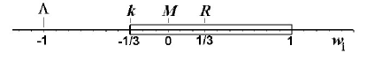
Figure 1: The range in $w_{i}$ is shown (in the box) for which the species satisfies the classical energy conditions. Here $M$ stands for dust ($w_{M}=0$) and $R$ for radiation ($w_{R}=1/3$).

It follows from (6) that

$$2q-1=3\sum_{i}w_{i}\Omega_{i}$$ (9)

and writing $1+z\equiv\frac{a_{0}}{a}$ nophotons , it also follows that

$$\Omega_{i}=\frac{(1+z)^{3(1+w_{i})}\Omega_{io}}{\sum_{j}\Omega_{jo}(1+z)^{3(1+w_{j})}}.$$ (10)

As $1+z\rightarrow\infty$ (Big Bang or Big Crunch) it follows that $\Omega_{i}\rightarrow 0$ for all species except that with the largest $w_{i}>-1$. Then $\Omega_{i}\rightarrow 1$. As $1+z\rightarrow 0$, $\Omega_{i}\rightarrow 0$ for all species except that with the smallest $w_{i}\leq-1$. Then $\Omega_{i}\rightarrow 1$. From (9) and (10) it follows that the evolution of the universes considered are governed by the autonomous (but non-linear) system dynamical

$$\Omega_{i}^{{}^{\prime}}=\Omega_{i}((2q-1)-3w_{i})$$ (11)

where ${}^{{}^{\prime}}\equiv-(1+z)\frac{d}{d(1+z)}$.

III Solving the Friedmann equation

We solve the system (11) algorithmically by way of the construction of a complete set of constants of the motion. Consider all species or any subset thereof. To distinguish this latter possibility we replace $i$ by $\alpha$. A constant of the motion, defined globally over the history of a universe, and not with respect to any particular observer, is defined here to be a function

$$\mathcal{F}=\mathcal{F}(\Omega_{\alpha})$$ (12)

for which

$$\mathcal{F}^{\;{}^{\prime}}=0.$$ (13)

Consider the product

$$\mathcal{F}=\prod_{\alpha}\Omega_{\alpha}^{v_{\alpha}}$$ (14)

where the exponents $v_{\alpha}$ are constants. Note that we do not make use of (7) at this stage. For (13) to hold for (14), it follows from (11) that

$$(2q-1)V=3W$$ (15)

where

$$V\equiv\sum_{\alpha}v_{\alpha},\;\;\;W\equiv\sum_{\alpha}w_{\alpha}v_{\alpha}.$$ (16)

If $V\neq 0$ then according to (15) $q$ itself is a constant and so from (11) for each species the evolution is given by

$$\Omega_{i}=\Omega_{io}(1+z)^{1-2q+3w_{i}}.$$ (17)

We do not consider this case further here. If $q$ is not constant then for $\mathcal{F}$ of the form (14) to be a constant of the motion it follows from (15) that

$$V=W=0$$ (18)

and the constant itself then reduces to

$$\mathcal{F}=\prod_{\alpha}\mathcal{C}_{\alpha}^{v_{\alpha}}.$$ (19)

Sums, differences, products and quotients of constants of the motion are of course constants as well and so the range in $\alpha$ must be examined. First consider two species, say $\alpha=a,b$. It then follows form (18) that $w_{a}=w_{b}$ which is not possible as we require that the species be distinguished by $w$. Next suppose that $\alpha$ ranges over more than three species. It now follows from (18) that any such constant can be reduced to products and quotients of constants involving only three distinct species. As a result we need consider only those constants $\mathcal{F}$ constructed from three distinct species which we now do.

The trivial case is that of a universe for which there are only three species, say $a,b,$ and $c$. Then $\mathcal{F}=\Omega_{a}^{v_{a}}\Omega_{b}^{v_{b}}\Omega_{c}^{v_{c}}$ and since we can always choose $v_{a}$, (18) reduces to two equations in two unknowns. The constant of motion is then determined up to the choice in $v_{a}$. For example, with dust we have the species $\Lambda,M$ and $k$ (assumed $\neq 0$ two , the $\Lambda$CDM model) and it follows immediately that alpha

$$\mathcal{F}=\frac{\Omega_{\Lambda}\Omega_{M}^{2}}{\Omega_{k}^{3}}.$$ (20)

We can now substitute for $\Omega_{k}$ from (7).

More generally, consider $n$ species, $n>3$. If, say, species $a$ and $b$ are chosen to construct $\mathcal{F}$ then there are $n-2$ choices for the remaining species, the number of independent constants of the motion. Further, for example, there are $(n-2)(n-3)/2$ dependent constants of motion that follow which involve $a$ but not $b$. In any event, as with the case of only three species, since we can always specify one exponent, (18) always reduces to two equations in two unknowns.

As the foregoing algorithm makes clear, if species are added to a model, but none taken away, the constants of motion are inherited from the simpler model. For example, irrespective of what we add to the $\Lambda$CDM model, $\mathcal{F}$, given by (20), remains a constant of the motion.

Now consider evolution in a three dimensional subspace, say $\Omega_{a},\Omega_{b},\Omega_{c}$. We can construct the constant $\mathcal{F}_{1}=\Omega_{a}\Omega_{b}^{v_{b}}\Omega_{c}^{v_{c}}$, and the constant $\mathcal{F}_{2}=\Omega_{a}^{\bar{v}_{a}}\Omega_{b}^{\bar{v}_{b}}\Omega_{d}$ where $d$ is any species other than $a,b$ or $c$. Then with (7) we replace $\Omega_{d}$. All species other than $a,b$ or $c$ that now enter are replace with the aide of constants constructed from that species and any two of $a,b$ and $c$. In the subspace then we have two independent relations that relate $\Omega_{a},\Omega_{b},\Omega_{c}$. The intersection of these surfaces in the subspace defines the evolution trajectory of the associated universe in that subspace.

To amplify the foregoing, consider, for example, dust and radiation. We have the species $\Lambda,M,R$ and $k$ (assumed $\neq 0$). Following the algorithm outlined above we immediately obtain the constants rindler

$$\mathcal{F}_{1}=\frac{\Omega_{\Lambda}\Omega_{M}^{2}}{\Omega_{k}^{3}},\;\;\;\mathcal{F}_{2}=\frac{\Omega_{\Lambda}\Omega_{R}^{3}}{\Omega_{M}^{4}},$$ (21)

$$\mathcal{F}_{3}=\frac{\Omega_{\Lambda}\Omega_{R}}{\Omega_{k}^{2}},\;\;\;\mathcal{F}_{4}=\frac{\Omega_{k}\Omega_{R}}{\Omega_{M}^{2}}.$$ (22)

First note that the constant $\mathcal{F}_{1}$ is inherited from the $\Lambda$CDM model as discussed above. Moreover, only two of the above constants are independent. For example, $\mathcal{F}_{3}=\mathcal{F}_{1}\mathcal{F}_{4}$ and $\mathcal{F}_{2}=\mathcal{F}_{1}\mathcal{F}_{4}^{3}$. In, say, the $\Lambda,M,R$ subspace the history of a universe is obtained by the trajectory defined by the intersection of $\mathcal{F}_{2}$ with one of the other constants and with $\Omega_{k}$ replaced by $1-\Omega_{\Lambda}-\Omega_{M}-\Omega_{R}$ in that constant further .

We end our discussion of constants of the motion here by noting that there are an infinite number of universes, of arbitrary complexity (but containing the species $\Lambda,M$ and $k$), for which

$$\frac{\Omega_{k}^{3}}{\Omega_{\Lambda}\Omega_{M}^{2}}\sim 0$$ (23)

throughout the entire history of the universe. The fact that we would appear to live in such a universe is a problem for some cosmologists - the “flatness problem”. We take the view that this “problem” arises only when too few species are considered, in the limit a two species model with only $M$ and $k$, in order to put the issue in perspective.

Central to the discussion given above is the system (11). We now discuss how this system can be used to make a fundamental distinction between model universes.

IV The gravitational epoch function

In rigorous texts on general relativity, for example O'Neill and Sachs , spacetime is defined (in part) as a time-oriented manifold. As stated in O'Neill , time-oriented is often weakened simply to time-orientable, and as pointed out in Sachs , the local time orientation is, with guesswork, extrapolated to the universe as a whole. Here we take a gravitational epoch function to be defined as a scalar field constructed from dimensionless ratios of invariants, each derivable from the Riemann tensor without differentiation, such that the function is monotone throughout the history of the universe. The purpose of an epoch function is to allow the ordering of events without reference to any specific class of observers or, of course, coordinates. The existence of an epoch function, when unique, allows the rigorous time-orientation of an entire manifold without guesswork. This is why the existence of an epoch function is interesting.

In a conformally flat four dimensional spacetime the maximum number of independent scalar invariants derivable from the Riemann tensor without differentiation is four. These are usually taken to be the Ricci scalar $R$ at degree $d=1$ and the Ricci invariants $r(d-1)$ for $d=2,3,4$. (Degree ($d$) here means the number of tensors that go into the construction of the scalar. Let $R_{abcd}$ signify the Riemann tensor, $R_{a}^{b}$ the Ricci tensor, $R$ the Ricci scalar ($\equiv R_{a}^{a}$) and $S_{a}^{b}$ the trace-free Ricci tensor ($\equiv R_{a}^{b}-\frac{R}{4}\delta_{a}^{b}$). The Ricci invariants are defined by (the coefficients are of no physical consequence as they derrive from the spinor forms of the invariants): $r(1)\equiv\frac{1}{2^{2}}S_{a}^{b}S^{a}_{b}$, $r(2)\equiv-\frac{1}{2^{3}}S_{a}^{b}S_{b}^{c}S_{c}^{a}$, and $r(3)\equiv\frac{1}{2^{4}}S_{a}^{b}S_{b}^{c}S_{c}^{d}S_{d}^{a}$. The Kretschmann invariant, for example, is not used since $6R_{abcd}R^{abcd}=R^{2}+48r(1)$ in the conformally flat case.) The dimension of these invariants is $L^{-2d}$. In a Robertson - Walker spacetime only two of these invariants are independent and in this spacetime it follows that $r(1)^{2}/r(3)=12/7,\,r(1)^{3}/r(2)^{2}=3,\,R^{4}/r(3)=12f^{2}/7$ and $(R^{3}/r(2))^{2}=3f^{3}$ where

$$f\equiv\frac{R^{2}}{r(1)}.$$ (24)

It is clear that $f$ given by (24), or any monotone function thereof, is the only epoch function that can be constructed in a Robertson - Walker spacetime. Universes can then be fundamentally categorized as to whether or not they admit monotone $f$.

For convenience consider $\mathcal{T}\equiv f/48$. It follows directly that in any Robertson - Walker spacetime

$$\mathcal{T}=(\frac{\Omega_{k}+q-1}{\Omega_{k}-q-1})^{2}.$$ (25)

Whereas $\mathcal{T}$ is defined through a bounce, its representation in the $\Omega$ notation is not. This is of no concern here since we are concerned with the behaviour of $\mathcal{T}$ strictly prior to any bounce should one exist. With the aide of (11), applied only to the species $k$, it also follows that

$$\mathcal{T}^{\;{}^{\prime}}=\frac{4(\Omega_{k}+q-1)(-2q^{2}\Omega_{k}+q^{{}^{\prime}}(\Omega_{k}-1))}{(\Omega_{k}-q-1)^{3}}.$$ (26)

If we now apply the restriction (5) and use the full set of equations (11) it follows that in addition to (9)

$$q^{\;{}^{\prime}}=\frac{9}{2}((\sum_{i}w_{i}\Omega_{i})^{2}-\sum_{i}w_{i}^{2}\Omega_{i}).$$ (27)

Let us again consider the $\Lambda$CDM model rad . It follows from (25) that

$$\mathcal{T}=(\frac{\Omega_{M}+4\Omega_{\Lambda}}{3\Omega_{M}})^{2}$$ (28)

and from (26) and (27) that

$$\mathcal{T}^{\;{}^{\prime}}=8\Omega_{\Lambda}(\frac{\Omega_{M}+4\Omega_{\Lambda}}{3\Omega_{M}^{2}})$$ (29)

and finally from (11) applied to $M$ and $\Lambda$ that

$$\mathcal{T}^{\;{}^{\prime\prime}}=8\Omega_{\Lambda}(\frac{\Omega_{M}+8\Omega_{\Lambda}}{\Omega_{M}^{2}}).$$ (30)

As a result, $\mathcal{T}$ has a global minimum value of $0$ when

$$\Omega_{\Lambda}=-\frac{\Omega_{M}}{4}.$$ (31)

The question then is, what $\Lambda$CDM models intersect the locus (31) and therefore fail to have $\mathcal{T}$ monotone degenerate ?

Since $\Omega_{M}>0$ clearly all $\Lambda$CDM models with $\Lambda>0$ admit the epoch function (28). Now consider $\Lambda<0$. For $k=0$ condition (31) holds at $(\Omega_{M},\Omega_{\Lambda})=(4/3,-1/3)$. For $k\neq 0$ use (31) in (20) to define

$$\mathcal{F}_{int}=\frac{16\Omega_{M}^{3}}{(3\Omega_{M}-4)^{3}}.$$ (32)

With $k=-1$ choose a value of $\Omega_{M}$ in the range $0<\Omega_{M}<4/3$ and insert this value into (32). The resultant $\mathcal{F}_{int}$ (which is negative) is the constant of motion associated with the intersection of the associated integral curve with the locus (31) with the intersection taking place at the chosen value of $\Omega_{M}$. For $k=1$ choose a value of $\Omega_{M}$ in the range $4/3<\Omega_{M}<\infty$ and follow the foregoing procedure ($\mathcal{F}_{int}$ is now positive). However, with $k=1$, as $\Omega_{M}\rightarrow\infty$ the constant $\mathcal{F}_{int}$ reaches the lower bound of $16/27$. There is then the range $0<\mathcal{F}<16/27$ for which the associated integral curves do not intersect the locus (31). We conclude then that for the $\Lambda$CDM models, all models with $\Lambda>0$ admit the epoch function (28), but for $\Lambda<0$ only those with $k=1$ and $0<\mathcal{F}<16/27$ do. There is no evidence that our universe lies in this latter category. Indeed, all the current evidence would suggest that we are very far away from it.

We now make some general observations on the monotonicity of $\mathcal{T}$, but restricted to the case $\Omega_{k}=0$ furthert . In this case it follows from (26) that the monotonicity of $\mathcal{T}$ is closely associated with the monotonicity of $q$. For example, if we assume that $q$ is monotone decreasing, then we can put a limit on the maximum $w$ allowed for a monotone $\mathcal{T}$. To do this note that for models with a Big Bang the initial value of $q$ is $(3\tilde{w}+1)/2$ where $\tilde{w}$ signifies the largest value of $w$ (assumed $>-1$) for all species. It follows from (26) then that $\mathcal{T}$ can be monotone only for $\tilde{w}\leq 1/3$. In view of (8) this is a rather surprising restriction, but one which is in accord with all observations.

V Summary

A complete set of constants of the motion has been constructed for all FLRW models consisting of an arbitrary number of separately conserved species, each with a constant ratio of pressure to density. These constants of the motion are to be considered as the fundamental characteristics of the model universes. The unique candidate for a gravitational epoch function has been constructed for all FLRW models. In the simplest of all models, the $\Lambda$CDM model, it has been shown that the epoch function exists for all models with $\Lambda>0$, for no models with $\Lambda=0$, and for almost no models with $\Lambda<0$. This function allows the global ordering of events without reference to any particular class of observers or, of course, coordinates.

- (1) Electronic Address: lake@astro.queensu.ca
- (2) To sight just two recent examples, see A. Clocchiatti et al., Ap. J. 642, 1 (2006) astro-ph/0510155 and P. Astier et al., Astronomy and Astrophysics 447, 31 (2006) astro-ph/0510447
- (3) For recent discussions see, for example, R. Bean, S. Carroll and M. Trodden astro-ph/0510059, T. Padmanabhan astro-ph/0603114, C. Seife, Science 309, 78 (2005), A. Albrecht et al. astro-ph/0609591
- (4) Compare, for example, M. V. John, Ap. J. 614, 1 (2004) astro-ph/0406444
- (5) D. Lovelock, J. Math. Phys. 13, 874 (1972).
- (6) The classical energy conditions include the weak, strong, null and dominant energy conditions. See, for example, S. W. Hawking and G. F. R. Ellis, The Large Scale Structure of Space-Time (Cambridge University Press, Cambridge, 1973), M. Visser, Lorentzian Wormholes (Springer-Verlag, New York, 1996) and E. Poisson, A Relativist’s Toolkit: The Mathematics of Black-hole Mechanics (Cambridge University Press, Cambridge, 2004).
- (7) We are not considering the propagation of photons but still use the familiar notation. In particular, we can set .
- (8) The dynamical systems approach is well developed in mathematical cosmology and most of what has been given so far is known. See J. Wainwright and G. F. R. Ellis, Dynamical Systems in Cosmology (Cambridge University Press, Cambridge, 1997) and for a complementary work, covering a different selection of topics, see A. A. Coley, Dynamical Systems and Cosmology (Kluwer Academic, Dordrecht, 2003). For a pedagogical study (restricted to three species) see J-P. Uzan and R. Lehoucq, Eur. J. Phys. 22, 371 (2001).
- (9) The case of two species is completely determined by (7).
- (10) This is the constant (sign, ) that I have used to discuss the flatness problem previously. See, K. Lake, Phys. Rev. Lett. 94, 201102 (2005) astro-ph/0404319. At the time I was unaware of the interesting work by U. Kirchner and G. F. R. Ellis, Class. Quantum Grav. 20, 1199 (2003) who also use a constant of motion, the notation being related simply by . The earliest use of this constant I have since found is in Appendix C of P. T. Landsberg and D. A. Evans, Mathematical Cosmology (Oxford University Press, Oxford, 1977). It follows, after some algebra, that the notation is related simply by .
- (11) The constants and have been given previously. See J. Ehlers and W. Rindler, Mon. Not. R. astr. Soc 238, 503 (1989). In their notation, and .
- (12) S. Guha and K. Lake (in preparation).
- (13) B. O’Neill, Semi-Riemannian Geometry (Academic Press, New York, 1983).
- (14) R. K. Sachs and H. Wu, General Relativity for Mathematicians (Springer-Verlag, Berlin, 1977).
- (15) The results when the species is also included are somewhat similar. See further .
- (16) Since for we consider the associated spacetimes time-unoriented.
- (17) For a more detailed analysis see K. Lake (in preparation).