Group field theory formulation of 3d quantum gravity coupled to matter fields

Abstract

ABSTRACT

We present a new group field theory describing 3d Riemannian quantum gravity coupled to matter fields for any choice of spin and mass. The perturbative expansion of the partition function produces fat graphs colored with $SU(2)$ algebraic data, from which one can reconstruct at once a 3-dimensional simplicial complex representing spacetime and its geometry, like in the Ponzano-Regge formulation of pure 3d quantum gravity, and the Feynman graphs for the matter fields. The model then assigns quantum amplitudes to these fat graphs given by spin foam models for gravity coupled to interacting massive spinning point particles, whose properties we discuss.

I Introduction

I.1 Background

Spin foam models daniele ; alex emerged recently as a general formalism for quantum gravity, and a point of convergence of different approaches, including loop quantum gravity (of which they may be thought of as a path integral formulation), topological field theories using ideas from category theory, and simplicial gravity. They assign geometric data to the simplicial spacetime in an algebraic form. In turn, spin foam models have been shown to be obtainable from so-called group field theories iogft ; laurentgft , i.e. field theories over group manifolds that can be seen as a generalisation of matrix models in that they produce, in their perturbative expansion in Feynman graphs, a sum over simplicial complexes of dimension higher than 2, with the configuration/momentum variables of the field being interpreted as geometric data for these complexes. This sum over simplicial complexes constructed as Feynman diagrams of the group field theory, implies also a sum over topologies; therefore the group field theory formalism can be interpreted laurentgft ; iogft as a realization of a third quantization of gravity at the simplicial level. There exist promising and currently much studied spin foam models, and group field theories, in 4-dimensions daniele ; alex , whose validity is, however, still under investigation. In the simpler case of 3-dimensional gravity (both Riemannian and Lorentzian, with and without cosmological constant) it is now established that spin foam models provide a consistent quantization, equivalent, but also presenting distinctive advantages, to those obtained from other approaches. The relevant model for 3d gravity without cosmological constant is the Ponzano-Regge model laurentPRI , whose group field theory derivation was given by Boulatov in boulatov .

The coupling of matter fields to quantum gravity in the spin foam framework is of paramount importance for various reasons, apart from the obvious one that for a consistent theory of quantum gravity to be correct, it should be able to describe in full the interactions between gravity and matter fields. First of all, matter coupling may provide the best, if not the only, way to define quantum observables for the theory that have a clear physical meaning, given that such observables are very difficult to define in a pure gravity theory carloObs ; carlopartial ; bianca . In particular, the inclusion of matter fields may prove to be the main avenue towards the construction of a quantum gravity phenomenology that could be put to test in future experiments amelino , the idea being that quantum gravity will modify the usual dynamics of matter fields (e.g. dispersion relations, scattering amplitudes, etc.) even in an approximately flat background, leading to potentially testable effects. Also, it is hoped that quantum gravity will not only modify the usual predictions of quantum field theory, but also solve various problems of the same, including that of ultraviolet divergences, providing a kind of built-in covariant cut-off at the Planck scale. Whether any of these hopes are actually fulfilled can be shown only by explicit work on matter couplings in quantum gravity models, including spin foams. Recently much research has been devoted to this issue. After some more speculative proposals crane ; lee ; mikovic , a spin foam model for gravity coupled to gauge fields in 4d has been constructed in danhend , and later re-derived using different methods in mikovicgauge , but most of the work on matter fields in spin foam models for quantum gravity has been done in the past two years KarimAlex ; barrettfeynman ; laurentPRI ; laurentPRII ; laurentPRIII and focused on the 3d case. The work of KarimAlex , starts off from a canonical perspective and build on results that have been obtained in the context of loop quantum gravity carlo-hugo ; kirill ; kirill-john ; thomas , and obtains a spin foam description of the dynamics of matter and quantum gravity by an explicit construction of the projector onto physical quantum states of the coupled system. On the other hand the construction of laurentPRI ; laurentPRII ; laurentPRIII uses a covariant/path integral picture from the start and is phrased in a discrete (simplicial) context. It is then more directly linked both in terms of language used and results obtained to the group field theory context. In fact, in this paper we are going to construct a group field theory whose corresponding Feynman amplitudes are exactly the spin foam amplitudes for gravity coupled to particles of any spin derived in laurentPRI and further analysed in laurentPRII ; laurentPRIII . The basic ideas of the construction in laurentPRI are the following: 1) Feynman graphs for particle interactions (like those coming from usual quantum field theories), including their coupling with gravity, can be considered as (non-local) observables for quantum gravity, and therefore treated as such, i.e. inserted as appropriate operators in the pure gravity partition function, so that the theory would allow the computation of their expectation value; the formal expression of this expectation value is that of a modified spin foam model where the modified amplitudes encode both the geometric and particle degrees of freedom; 2) matter arises as a kind of symmetry-breaking singular configuration of the gravitational field, in the sense that pure gauge degrees of freedom are turned into physical degrees of freedom (characterizing matter) at the location of the particles. We will see in the following how these ideas are realised also in our model at the group field theory level. In particular, the first idea has a very natural implementation in the group field theory formalism (in a sense, it suggests such a formalism) and it is rather new and likely to be a key for future developments towards quantum gravity phenomenology, thanks to the possibility of extracting an effective non-commutative field theory for matter fields encoding the quantum gravity effects laurentPRIII . On the other hand, the idea of matter as a topological defect of gravity in 3d is well-established since the work of S. Deser, R. Jackiw, and G. ’t Hooft DJT ; matschullwelling both at the classical and quantum continuum level, but finds a beautiful purely algebraic and combinatorial realisation in the spin foam construction of laurentPRI , and therefore in the present work. A similar use of Feynman graphs as observables for quantum gravity, as a basis for studying the coupling of matter fields to it, was done in barrettfeynman in the context of the Turaev-Viro spin foam model for 3d gravity with cosmological constant, where the diagrams considered included colored knots. It is of great importance for the group field theory programme laurentgft ; iogft to be able to include matter couplings in it, and reproduce the known coupled spin foam models, in order to be entitled to consider it a fundamental definition of a theory of quantum gravity, and in particular as the truly fundamental definition of spin foam models themselves, rather than just an auxiliary formalism. Work on a group field theoretic description of quantum gravity coupled to matter fields has started only very recently, the first constructions having been presented in kirillgft and us . In kirillgft a very elegant extension of the Boulatov group field theory model for 3d quantum gravity to the $DSU(2)$ quantum group is performed, motivated by the fact that the coupled spin foam amplitudes of laurentPRI present a symmetry under this particular deformation of the Poincare’ group laurentPRII and that particle states result in being labeled by $DSU(2)$ representations. However, the resulting model does not have a clear interpretation in terms of particle configurations. Still in kirillgft a new class of spin foam models admitting such interpretation is constructed using chain mail techniques (see also laurentPRII ), but with no derivation of the same from group field theories. In us a group field theory that produces spin foam amplitudes for matter coupled to 3d gravity was proposed, and shown to reproduce the amplitudes of laurentPRI in the special case of massive scalar particles/fields (more precisely, for particles with no spin nor angular momentum). The model we present in this paper can be seen as a generalisation and an appropriate modification of that proposed in us ; it does not only generalise it to the case of spinning matter fields and generic interaction, but it also uses a simpler formalism with a clearer physical interpretation, as we will show in the following. This is not a direct generalisation, however, in the sense that even in the particular case of spinless particles it provides an alternative way to couple matter to gravity in group field theory, as we will see in the following. We believe that the model in us has a very interesting structure and that its peculiar features deserve further investigation.

I.2 The new GFT model: general ideas

Let us summarise and introduce the main ideas behind our model. Of course, all of the following will be made precise and explicit later in this work. The spin foam model of laurentPRI , as we mentioned above, is based (as is the work of barrettfeynman ) on the idea that one should couple a full history of particle interactions and evolution, represented by a Feynman diagram of the type produced by matter field theories, to a history of the gravitational field represented by a spin foam, and define an appropriate quantum amplitude for the composite history. Now, the spin foam itself is just a specific Feynman diagram for the group field theory so that the coupled spin foam is best interpreted as a Feynman diagram for both gravity and matter fields and this leads naturally to the search for the modified group field theory that generates it in its perturbative expansion. This means that we want to realise the third quantization of gravity in a simplicial setting and the second quantization of matter living on the same simplicial structures in one stroke, and define a field theory on a group manifold that produces at once, in perturbative expansion, a sum over spacetimes and geometries and a sum over Feynman diagrams for matter interactions, understood as taking place in such spacetimes. As for the representation of matter degrees of freedom, we base ourselves on the extensive knowledge of matter in 3d gravity coming from both continuum classical analyses DJT , loop quantum gravity KarimAlex and spin foams laurentPRI . By virtue of its spin (and angular momentum), a particle breaks locally the gauge invariance of pure gravity, so that the $SU(2)$ gauge degrees of freedom are turned into physical degrees of freedom of the particle at its location. This is a kinematical feature that is evident before any dynamics are imposed. In the framework of loop quantum gravity, and thus for what concerns the boundary states of spin foam models, this implies that the relevant combinatorial/algebraic structures describing states of the gravity+matter system are open spin networks with one loose end labelled by the spin of the particle; one can thus encode the presence of a particle in the spin network describing a boundary state of a spin foam model by replacing one of its 3-valent vertices (in 3d) with a 4-valent vertex having an extra loose link labelled with the particle data. In the dual simplicial geometric interpretation of spin networks in a spin foam context, this means that one is replacing a triangle on the boundary of the simplicial 3-manifold dual to the spin foam, with a modified triangle carrying a particle and thus possessing a modified geometry. In the simplicial third quantization provided by the group field theory the object that corresponds to a geometric triangle is the field itself, so the starting idea for extending the setting to include spinning particles is to allow for a different type of field with a modified combinatorial structure and a modified gauge symmetry, as we will see. The mass of the particles can be dealt with at the dynamical level, since it does not influence the kinematics of the fields, and should manifest itself by producing locally a deviation from the pure gravity flatness constraint at the location of the particle, i.e. as the presence of distributional curvature or a conical singularity along the particle trajectories. In other words, we are going to encode the presence of a massive particle in its interaction with the gravitational field. So we modify the interaction term of the pure gravity group field theory to include extra terms describing both the interaction of matter fields among themselves (modified by the gravity degrees of freedom), and the propagation of these matter fields in the quantum gravity background, effected by the generation of curvature along the particle trajectory, again following laurentPRI .

The end result is a field theory whose perturbative expansion gives fat graphs, as in the pure gravity case, but with extra combinatorial structures and algebraic data, so that one can identify from them both a labelled 2-complex that allows to reconstruct a 3d triangulation, its geometry and a Feynman graph for the interacting matter fields (of any spin and mass) alongside it. The quantum amplitudes for these fat graphs then describe how the matter field Feynman graphs are embedded in the simplicial complex and assign a total probability amplitude to the gravity plus matter configuration, that coincide with the amplitudes constructed in laurentPRI .

II The model

To recapitulate, the main aim for this section is to construct a group field theory with the following hallmark: when we expand its partition function, the sum over Feynman diagrams contains a sum over spin foams for matter coupled to gravity. These spin foam amplitudes were obtained recently from a path integral quantisation of first order gravity coupled to relativistic point particles (with arbitrary spin) laurentPRI . Results and properties of this model are outlined in Appendix A, and we will refer to these spin foam amplitudes as Coupled Ponzano-Regge (CPR) amplitudes.

In conventional field theory, we usually distinguish between kinematic (field and symmetries) and dynamic structures (action, partition function, etc). We follow a similar route here.

The outline of this section is as follows: we begin by defining the fields and their symmetries and show how they incorporate the kinematic scene; later, we define an action and examine its dynamic input; finally, we provide a more in-depth discussion of generic Feynman amplitudes to link back to the spin foam stage.

II.1 Classical and quantum kinematics

We divide our exploration of the kinematic sector into two parts: pure gravity and matter coupled to gravity, dealing with both in a similar way.

We describe the pure gravity sector of our theory using the field arising in Boulatov’s field theory boulatov . This theory is a GFT for 3d Riemannian quantum gravity: its Feynman diagrams are Ponzano-Regge (PR) spin foams associated to 3-(pseudo)manifolds. The sum in the expansion of the partition function is over all geometries for given topology and chosen triangulation (that is, over all triangulations for given topology), as well as over all topologies. Since the PR amplitude is a topological invariant it does not depend on the geometry. First of all, the field is defined as a map from the Cartesian product of three copies of $\mathrm{SU}(2)$ to the complex numbers:

$$\phi:\mathrm{SU}(2)\times\mathrm{SU}(2)\times\mathrm{SU}(2)\rightarrow\mathbb{C};\quad\phi(g_{1},g_{2},g_{3}).$$ (1)

We refer to this field as the Boulatov field. It has two symmetries:

• we require $\phi$ to be invariant under (even) elements $\sigma$ of the permutation group of three elements $S_{3}$, acting on the field variables,

  $$\phi(g_{1},g_{2},g_{3})=\phi(g_{\sigma(1)},g_{\sigma(2)},g_{\sigma(3)}),$$ (2)

  the Feynman amplitudes produced by the corresponding group field theory are in one-to-one correspondence with orientable 2-complexes, as explained in dfkr ; dep ; odd permutations map this field to its complex conjugate;

• we require the field to be Lorentz invariant; we ensure this by projecting the field onto its $\mathrm{SU}(2)$ invariant part:

  $$P_{\alpha}\phi(g_{1},g_{2},g_{3})\equiv\int_{\mathrm{SU}(2)}d\alpha\;\phi(g_{1}\alpha,g_{2}\alpha,g_{3}\alpha).$$ (3)

Now that we have defined the field and its symmetries we want to recover a full understanding of how these structures relate to the kinematic regime. We then expand this field into its Fourier modes by means of a Peter-Weyl decomposition. This gives a field dependence on three irreducible representations, one corresponding to each copy of $\mathrm{SU}(2)$. We perform the expansion on the projected field in Appendix B explicitly and the result is:

$$P_{\alpha}\phi(g_{1},g_{2},g_{3})=\sum_{\begin{subarray}{c}j_{i},m_{i},n_{i}\\ 1\leq i\leq 3\end{subarray}}\sqrt{d_{j_{1}}d_{j_{2}}d_{j_{3}}}\Phi^{j_{1}\;\;j_{2}\;\;j_{3}}_{m_{1}m_{2}m_{3}}D^{j_{1}}_{m_{1}n_{1}}(g_{1})D^{j_{2}}_{m_{2}n_{2}}(g_{2})D^{j_{3}}_{m_{3}n_{3}}(g_{3})C^{j_{1}\;j_{2}\,j_{3}}_{n_{1}n_{2}n_{3}},$$ (4)

where $D$ is a representation matrix of $\mathrm{SU}(2)$, $C$ is an $\mathrm{SU}(2)$ $3j$-symbol and $d_{j}$ is the dimension of the $j$ representation. Furthermore, the field $\Phi$ has the symmetries of an $\mathrm{SU}(2)$ $3j$-symbol.

The group field theory formalism is a path integral formulation and transition amplitudes arise as ‘two-point’ functions where the two ‘points’ are possible boundary data of the theory. The states have the same structure as spin network functionals. These are ‘coloured’ closed trivalent graphs, where the edges are labelled by matrix elements $D^{j}_{mn}(g)$ of the holonomy $g$ along the edge in a fixed representation $j$ and the vertices are labelled by invariant intertwiners $C^{j_{1}\;j_{2}\,j_{3}}_{n_{1}n_{2}n_{3}}$ contracting the matrices. Thus a single vertex and its three incident edges are given by

$$D^{j_{1}}_{m_{1}n_{1}}(g_{1})D^{j_{2}}_{m_{2}n_{2}}(g_{2})D^{j_{3}}_{m_{3}n_{3}}(g_{3})C^{j_{1}\;j_{2}\,j_{3}}_{n_{1}n_{2}n_{3}},$$ (5)

which we recognise from (4) as constituting much of the Boulatov field. Indeed, we seek a way to translate the spin network functional into the language of group field theory. We accomplish this naturally by considering the same spin network graphs but with the edges now labelled by the fixed representation and the vertices by $\Phi^{j_{1}\;\;j_{2}\;\;j_{3}}_{m_{1}m_{2}m_{3}}$ which is indeed an invariant intertwiner. Thus a boundary state in the Boulatov model is a product of $\Phi$ fields reisenberger , contracted with respect to the ‘magnetic’ indices $m$, and diagrammatically represented by a spin network. This state charts the gravitational information of a 2d hypersurface.

Figure 1: The pure gravity field.

As for the geometric interpretation, in the kinematic arena, a spin network vertex is dual topologically to a triangle, the representations are related to its edge lengths and the intertwiner ensures that the triangle inequalities are satisfied; therefore, we think of the Boulatov field as representing a triangle in the triangulation of a boundary 2-manifold kinematically, and later of a 3-manifold dynamically.

There is a new field to represent the sector of our theory where matter couples to gravity. This field provides us with explicit information about the momentum and spin of the particle. These are the two quantities needed to thoroughly account for a point particle coupled to gravity. We define the field as a map from the Cartesian product of four copies of $\mathrm{SU}(2)$ to the complex numbers:

$$\psi_{s}(g_{1},g_{2},g_{3};u):\mathrm{SU}(2)\times\mathrm{SU}(2)\times\mathrm{SU}(2)\times\mathrm{SU}(2)\rightarrow\mathbb{C}.$$ (6)

We refer to $\psi_{s}$ as the coupled field. It has four arguments, the first three still encapsulate the gravitational degrees of freedom while the new fourth argument is related to the momentum of the particle. We perform a partial decomposition to clarify the definition of the field.

$$\qquad\psi_{s}(g_{1},g_{2},g_{3};u)=\sum_{I,n}\psi^{I}_{sn}(g_{1},g_{2},g_{3})D^{I}_{sn}(u).$$ (7)

The $s$ index is fixed and refers to the spin of the particle, the representation $I$ denotes its total angular momentum.

Also, the new field $\psi_{s}$ can be understood as the result of projecting a generic four-argument field $\psi$ to a specific spin component $s$ by means of a projector operator $P_{s}$ acting, on its fourth argument, as:

$$\psi_{s}(g_{1},g_{2},g_{3};u)=(P_{s}\psi)(g_{1},g_{2},g_{3};u)=\sum_{J}\int_{SU(2)}dgd_{J}D^{J}_{ss}(ug^{-1}\psi(g_{1},g_{2},g_{3};g).$$ (8)

We impose one symmetry on the field. This is Lorentz symmetry that is once again ensured by projection onto the $\mathrm{SU}(2)$ invariant part of the field, by simultaneous right action on all four arguments:

$$P_{\alpha}\psi_{s}(g_{1},g_{2},g_{3};u)\equiv\int_{\mathrm{SU}(2)}d\alpha\;\psi_{s}(g_{1}\alpha,g_{2}\alpha,g_{3}\alpha;u\alpha).$$ (9)

We will discuss later why we do not impose permutation symmetry and what consequences this has on the resulting Feynman amplitudes.

Once again we expand this field into its Fourier modes:

$$P_{\alpha}\psi_{s}(g_{1},g_{2},g_{3};u)=\sum_{\begin{subarray}{c}I,n,j_{i},m_{i},n_{i}\\ 1\leq i\leq 3\end{subarray}}\sum_{\Lambda}\sqrt{d_{j_{1}}d_{j_{2}}d_{j_{3}}d_{I}}\Psi^{j_{1}\;\;j_{2}\;\;j_{3}\;\,I\;\Lambda}_{m_{1}m_{2}m_{3}s}D^{j_{1}}_{m_{1}n_{1}}(g_{1})D^{j_{2}}_{m_{2}n_{2}}(g_{2})D^{j_{3}}_{m_{3}n_{3}}(g_{3})D^{I}_{sn}(u)\tilde{C}^{j_{1}\;j_{2}\,j_{3}\,I\,\Lambda}_{n_{1}n_{2}n_{3}n},$$ (10)

where $\tilde{C}$ is an invariant intertwiner of four representations, $\Lambda$ labels a basis in the space of 4-valent intertwiners and $\Psi$ has the symmetries of a 4-valent $SU(2)$ intertwiner.

We use our knowledge of the boundary states of the CPR spin foam model to explain the kinematic information contained in the coupled field. The boundary spin foam states for matter coupled to gravity are open coloured trivalent spin network functionals. That is, some edges do not join trivalent vertices but instead join a trivalent vertex to an endpoint. On these edges and endpoints reside the kinematic data of the particles. The edges are labelled with the matrix elements of the holonomy along that edge and at the endpoints are projected down to the spin-$s$ component. The matrix elements naturally furnish the particle arena with a Poincaré representation labelled by its spin and mass $(s,m)$:

$$V_{s,m}=\bigoplus_{I}\left\{D^{I}_{sn}(u):I-s\in\mathbb{N}\;;\;|n|\leq I\right\}.$$ (11)

In the Poincaré representation of a particle, $I$ labels the particle’s total angular momentum, $s$ its spin, and $u$ its momentum. Therefore, we label a trivalent vertex with an open edge and two normal edges with

$$D^{j_{1}}_{m_{1}n_{1}}(g_{1})D^{j_{2}}_{m_{2}n_{2}}(g_{2})D^{I}_{sn}(u)C^{j_{1}\;j_{2}\,I}_{n_{1}n_{2}n}.$$ (12)

To translate this state into the GFT language we want to consider the same open trivalent spin network and label the edges with representations and the trivalent vertices with fields, as we did in the pure gravity case. For those vertices with three normal edges, we can label them as before with the Boulatov field. For those special vertices with an open edge, we wish to label them with the coupled field $\Psi^{j_{1}\;\;j_{2}\;\;j_{3}\;I\,\Lambda}_{m_{1}m_{2}m_{3}s}$; this naturally labels a 4-valent vertex, which in turn can be decomposed into two trivalent vertices joined by a new intermediate edge that is labelled by the $\mathrm{SU}(2)$ representation $\Lambda$. Thus we use the coupled field to label two trivalent vertices: one normal and one special. In the end, a boundary state is given by a product of $\Phi$ and $\Psi$ fields, contracted according to the combinatorics of the graph. We view the $\psi_{s}$ field as a triangle with extra particle degrees of freedom on one of its vertices, as seen in FIG.2.

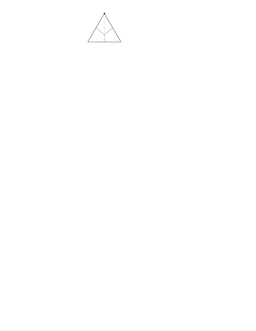
Figure 2: The coupled field.

II.2 Classical dynamics and kinetic and vertex terms

The action defines the classical dynamics of the fields. From this, one could calculate the classical equations of motion of the group field theory (i.e. Euler-Lagrange equations). The classical equations of motion of the Boulatov GFT describe the local evolution of pure quantum gravity in a simplicial setting, and a recent proposal by Freidel laurentgft , suggests that the classical structure of the GFT is what only matters for the definition of the inner product between canonical states in a GFT formulation of pure quantum gravity. Certainly, a similar interpretation is possible for our coupled GFT, and a parallel analysis should be carried out for the GFT model we propose here, so to unveil all the information about local evolution and canonical inner product for gravity coupled to matter, but we leave this for future work. We state our action as follows:

$$\begin{split}S[\phi,\psi_{s}]=&\;S_{gr}+S_{gr+mat}=S_{gr}+S_{gr+mat}^{kin}+S_{gr+mat}^{int-2}+S_{gr+mat}^{int-3}+S_{gr+mat}^{int-4}=\\ &\;=\frac{1}{2}\int\prod^{3}_{i=1}dg_{i}\;P_{\alpha}\phi(g_{1},g_{2},g_{3})P_{\bar{\alpha}}\phi(g_{1},g_{2},g_{3})\\ &+\frac{\lambda}{4!}\int\prod^{6}_{i=1}dg_{i}\;P_{\alpha_{1}}\phi(g_{1},g_{2},g_{3})P_{\alpha_{2}}\phi(g_{3},g_{5},g_{4})P_{\alpha_{3}}\phi(g_{4},g_{2},g_{6})P_{\alpha_{4}}\phi(g_{6},g_{5},g_{1})\\ &+\frac{1}{2}\int\prod^{3}_{i=1}dg_{i}\,du\;P_{\alpha}\psi_{s}(g_{1},g_{2},g_{3};u)P_{\bar{\alpha}}\psi_{s}(g_{1},g_{2},g_{3};u)\\ &+\mu_{2}\int\prod^{6}_{i=1}dg_{i}\,du_{a}\;P_{\alpha_{1}}\psi_{s}(g_{1},g_{2},g_{3}u_{a}^{-1}hu_{a};u_{a})P_{\alpha_{2}}\psi_{s}(g_{4}u_{a}^{-1}h^{-1}u_{a},g_{3},g_{5};u_{a})P_{\alpha_{3}}\phi(g_{4},g_{2},g_{6})P_{\alpha_{4}}\phi(g_{6},g_{5},g_{1})\\ &+\mu_{3}\int\prod^{6}_{i=1}dg_{i}\,du_{a}\,du_{b}\,du_{c}\;P_{\alpha_{1}}\psi_{s}(g_{1},g_{2},g_{3}u_{a}^{-1}hu_{a};u_{a})P_{\alpha_{2}}\psi_{s}(g_{4}u_{b}^{-1}h^{-1}u_{b},g_{3},g_{5};u_{b})P_{\alpha_{3}}\psi_{s}(g_{6},g_{4},g_{2}u_{c}^{-1}hu_{c};u_{c})\\ &\phantom{xxxxxxxxxx}\times P_{\alpha_{4}}\phi(g_{6},g_{5},g_{1})\delta(u_{a}^{-1}hu_{a}u_{b}^{-1}h^{-1}u_{b}u_{c}^{-1}hu_{c})\sum_{\begin{subarray}{c}I_{a},I_{b},I_{c}\\ n_{a},n_{b},n_{c}\end{subarray}}D^{I_{a}}_{sn_{a}}(u_{a})D^{I_{b}}_{sn_{b}}(u_{b})D^{I_{c}}_{sn_{c}}(u_{c})C^{I_{a}\,I_{b}\,I_{c}}_{n_{a}n_{b}n_{c}}\\ &+\mu_{4}\int\prod^{6}_{i=1}dg_{i}\,du_{a}\,du_{b}\,du_{c}\,du_{d}\;P_{\alpha_{1}}\psi_{s}(g_{1},g_{2},g_{3}u_{a}^{-1}hu_{a};u_{a})P_{\alpha_{2}}\psi_{s}(g_{4}u_{b}^{-1}h^{-1}u_{b},g_{3},g_{5};u_{b})\\ &\phantom{xxxxxxxxxx}\times P_{\alpha_{3}}\psi_{s}(g_{2}u_{d}^{-1}hu_{d},g_{6},g_{4};u_{c})P_{\alpha_{4}}\psi_{s}(g_{6},g_{4},g_{2};u_{d})\delta(u_{a}^{-1}hu_{a}u_{b}^{-1}h^{-1}u_{b}u_{c}h^{-1}u_{c}u_{d}^{-1}hu_{d})\\ &\phantom{xxxxxxxxxx}\times\sum_{\begin{subarray}{c}I_{a},I_{b},I_{c},I_{d},\Lambda\\ n_{a},n_{b},n_{c},n_{d}\end{subarray}}D^{I_{a}}_{sn_{a}}(u_{a})D^{I_{b}}_{sn_{b}}(u_{b})D^{I_{c}}_{sn_{c}}(u_{c})D^{I_{d}}_{sn_{d}}(u_{d})\tilde{C}^{I_{a}\,I_{b}\,I_{c}\,I_{d}\,\Lambda}_{n_{a}n_{b}n_{c}n_{d}},\end{split}$$ (13)

where $h\in U(1)$ encodes the mass of the particle. Furthermore, the first line of the equation gives a schematic form of the later terms. $S_{gr}$ symbolises the first two terms (pure gravity), and $S_{gr+mat}$ binds up the later four terms (matter coupled to gravity). We give each of the matter terms its own separate name, for example $S_{gr+mat}^{int-2}$ denotes a vertex term with a bivalent particle interaction. We explain this in more detail later.

We deal in Section II.3 with the nature of the quantum dynamics. In order to proceed down that road we need to state precisely a partition function based on this action, and furthermore to construct the Feynman diagrams we require Feynman rules. We specify these explicitly in the form of propagators and vertex operators which we extract from the kinetic and interaction terms in the action, a standard modus operandi in field theory. The split occurs as follows:

$$\begin{split}S[\phi,\psi_{s}]=&\;\frac{1}{2}\int\prod^{3}_{i=1}dg_{i}\,d\bar{g}_{i}\;\phi(g_{1},g_{2},g_{3})\phi(\bar{g}_{1},\bar{g}_{2},\bar{g}_{3})\mathcal{K}_{\phi}(g_{i},\bar{g}_{i})\\ &+\int\prod^{6}_{i=1}dg_{i}\,d\bar{g}_{i}\;\phi(g_{1},g_{2},g_{3})\phi(\bar{g}_{3},g_{5},g_{4})\phi(\bar{g}_{4},\bar{g}_{2},g_{6})\phi(\bar{g}_{6},\bar{g}_{5},\bar{g}_{1})\mathcal{V}_{\phi}(g_{i},\bar{g}_{i})\\ &+\frac{1}{2}\int dg_{i}\,d\bar{g}_{i}\,du\,d\bar{u}\;\psi_{s}(g_{1},g_{2},g_{3};u)\psi_{s}(g_{1},g_{2},g_{3};u)\mathcal{K}^{s}_{\psi}(g_{i},\bar{g}_{i},u,\bar{u})\\ &+\int\prod^{6}_{i=1}dg_{i}\,d\bar{g}_{i}\,du_{a}\,du_{b}\;\psi_{s}(g_{1},g_{2},g_{3};u_{a})\psi_{s}(g_{4},\bar{g}_{3},g_{5};u_{b})\phi(\bar{g}_{4},\bar{g}_{2},g_{6})\phi(\bar{g}_{6},\bar{g}_{5},\bar{g}_{1})\mathcal{V}^{s}_{2\psi}(g_{i},\bar{g}_{i},u_{a},u_{b})\\ &+\int\prod^{6}_{i=1}dg_{i}\,d\bar{g}_{i}\,du_{a}\,du_{b}\,du_{c}\;\psi_{s}(g_{1},g_{2},g_{3};u_{a})\psi_{s}(g_{4},\bar{g}_{3},g_{5};u_{b})\psi_{s}(g_{6},\bar{g}_{4},\bar{g}_{2};u_{c})\phi(\bar{g}_{6},\bar{g}_{5},\bar{g}_{1})\mathcal{V}^{s}_{3\psi}(g_{i},\bar{g}_{i},u_{a},u_{b},u_{c})\\ &+\int\prod^{6}_{i=1}dg_{i}\,d\bar{g}_{i}\,du_{a}\,du_{b}\,du_{c}\,du_{d}\;\psi_{s}(g_{1},g_{2},g_{3};u_{a})\psi_{s}(g_{4},\bar{g}_{3},g_{5};u_{b})\psi_{s}(\bar{g}_{2},g_{6},\bar{g}_{4};u_{c})\\ &\phantom{xxxxxxxxxxxxxxxx}\times\psi_{s}(\bar{g}_{6},\bar{g}_{5},\bar{g}_{1};u_{d})\mathcal{V}^{s}_{4\psi}(g_{i},\bar{g}_{i},u_{a},u_{b},u_{c},u_{d}).\end{split}$$ (14)

The operators above are the kinetic and interaction operators for the $\phi$ and $\psi$ fields, stated explicitly as:

$$\mathcal{P}_{\phi} \equiv \mathcal{K}_{\phi}^{-1}=\mathcal{K}_{\phi}=\int d\alpha\,d\bar{\alpha}\;\delta(\bar{g}_{1}\bar{\alpha}^{-1}\alpha g_{1}^{-1})\delta(\bar{g}_{2}\bar{\alpha}^{-1}\alpha g_{2}^{-1})\delta(\bar{g}_{3}\bar{\alpha}^{-1}\alpha g_{3}^{-1}),$$ (15)

$$\mathcal{V}_{\phi} = \frac{\lambda}{4!}\int\prod_{i=1}^{4}d\alpha_{i}\;\delta(\bar{g}_{1}\alpha^{-1}_{4}\alpha_{1}g_{1}^{-1})\delta(\bar{g}_{2}\alpha^{-1}_{3}\alpha_{1}g_{2}^{-1})\delta(\bar{g}_{3}\alpha^{-1}_{2}\alpha_{1}g_{3}^{-1})\delta(\bar{g}_{4}\alpha^{-1}_{3}\alpha_{2}g_{4}^{-1})$$ (16)

$$\hphantom{xxxxxxxxxxx}\times\delta(\bar{g}_{5}\alpha^{-1}_{4}\alpha_{2}g_{5}^{-1})\delta(\bar{g}_{6}\alpha^{-1}_{4}\alpha_{3}g_{6}^{-1}),$$

$$\mathcal{P}^{s}_{\psi} \equiv \mathcal{K}_{\psi}^{s\;\;-1}=\mathcal{K}^{s}_{\psi}=\int d\alpha\,d\bar{\alpha}\;\delta(\bar{g}_{1}\bar{\alpha}^{-1}\alpha g_{1}^{-1})\delta(\bar{g}_{2}\bar{\alpha}^{-1}\alpha g_{2}^{-1})\delta(\bar{g}_{3}\bar{\alpha}^{-1}\alpha g_{3}^{-1})\delta(\bar{u}\bar{\alpha}^{-1}\alpha u^{-1}),$$ (17)

$$\mathcal{V}^{s}_{2\psi} = \mu_{2}\int\prod_{i=1}^{4}d\alpha_{i}\;\delta(\bar{g}_{1}\alpha^{-1}_{4}\alpha_{1}g_{1}^{-1})\delta(\bar{g}_{2}\alpha^{-1}_{3}\alpha_{1}g_{2}^{-1})\delta(\bar{g}_{3}\alpha^{-1}_{2}\alpha_{1}u_{a}^{-1}hu_{a}g_{3}^{-1})\delta(\bar{g}_{4}\alpha^{-1}_{3}\alpha_{2}u_{b}^{-1}hu_{b}g_{4}^{-1})$$ (18)

$$\hphantom{xxxxxxxxxxx}\times\delta(\bar{g}_{5}\alpha^{-1}_{4}\alpha_{2}g_{5}^{-1})\delta(\bar{g}_{6}\alpha^{-1}_{4}\alpha_{3}g_{6}^{-1})\delta(u_{a}\alpha_{1}^{-1}\alpha_{2}u_{b}^{-1})$$

$$\mathcal{V}^{s}_{3\psi} = \mu_{3}\int\prod_{i=1}^{4}d\alpha_{i}\;\delta(\bar{g}_{1}\alpha^{-1}_{4}\alpha_{1}g_{1}^{-1})\delta(\bar{g}_{2}\alpha^{-1}_{3}\alpha_{1}g_{2}^{-1})\delta(\bar{g}_{3}\alpha^{-1}_{2}\alpha_{1}u_{a}^{-1}hu_{a}g_{3}^{-1})\delta(\bar{g}_{4}\alpha^{-1}_{3}\alpha_{2}u_{b}^{-1}hu_{b}g_{4}^{-1})$$ (19)

$$\phantom{xxxxxxxxxxxx}\times\delta(\bar{g}_{5}\alpha^{-1}_{4}\alpha_{2}g_{5}^{-1})\delta(\bar{g}_{6}\alpha^{-1}_{4}\alpha_{3}g_{6}^{-1})\delta(\alpha_{1}u_{a}^{-1}hu_{a}\alpha_{1}^{-1}\alpha_{2}u_{b}^{-1}h^{-1}u_{b}\alpha_{2}^{-1}\alpha_{3}u_{c}^{-1}hu_{c}\alpha_{3}^{-1})$$

$$\phantom{xxxxxxxxxxxxxxxxxxxxxx}\times\sum_{\begin{subarray}{c}I_{a},I_{b},I_{c}\\ n_{a},n_{b},n_{c}\end{subarray}}D^{I_{a}}_{sn_{a}}(u_{a}\alpha_{1}^{-1})D^{I_{b}}_{sn_{b}}(u_{b}\alpha_{2}^{-1})D^{I_{c}}_{sn_{c}}(u_{c}\alpha_{3}^{-1})C^{I_{a}\,I_{b}\,I_{c}}_{n_{a}n_{b}n_{c}},$$

$$\mathcal{V}^{s}_{4\psi} = \mu_{4}\int\prod_{i=1}^{4}d\alpha_{i}\;\delta(\bar{g}_{1}\alpha^{-1}_{4}\alpha_{1}g_{1}^{-1})\delta(\bar{g}_{2}\alpha^{-1}_{3}\alpha_{1}u_{d}^{-1}hu_{d}g_{2}^{-1})\delta(\bar{g}_{3}\alpha^{-1}_{2}\alpha_{1}u_{a}^{-1}hu_{a}g_{3}^{-1})\delta(\bar{g}_{4}\alpha^{-1}_{3}\alpha_{2}u_{b}^{-1}hu_{b}g_{4}^{-1})$$ (20)

$$\phantom{xxxxxxxx}\times\delta(\bar{g}_{5}\alpha^{-1}_{4}\alpha_{2}g_{5}^{-1})\delta(\bar{g}_{6}\alpha^{-1}_{4}\alpha_{3}g_{6}^{-1})\delta(\alpha_{1}u_{a}^{-1}hu_{a}\alpha_{1}^{-1}\alpha_{2}u_{b}^{-1}h^{-1}u_{b}\alpha_{2}^{-1}\alpha_{3}u_{c}h^{-1}u_{c}\alpha_{3}^{-1}\alpha_{4}u_{d}^{-1}hu_{d}\alpha_{4}^{-1})$$

$$\phantom{xxxxxxxxxxxxxxxx}\times\sum_{\begin{subarray}{c}I_{a},I_{b},I_{c},I_{d},\Lambda\\ n_{a},n_{b},n_{c},n_{d}\end{subarray}}D^{I_{a}}_{sn_{a}}(u_{a}\alpha_{1}^{-1})D^{I_{b}}_{sn_{b}}(u_{b}\alpha_{2}^{-1})D^{I_{c}}_{sn_{c}}(u_{c}\alpha_{3}^{-1})D^{I_{d}}_{sn_{d}}(u_{d}\alpha_{4}^{-1})\tilde{C}^{I_{a}\,I_{b}\,I_{c}\,I_{d}\,\Lambda}_{n_{a}n_{b}n_{c}n_{d}},$$

where $\mathcal{P}_{\phi}$ and $\mathcal{P}^{s}_{\psi}$ are the propagators for the field theory.

Before we describe in detail the type of amplitudes that arise once we implement the Feynman rules, let us expound the attributes of the individual terms.

The first two terms $S_{gr}$, with operators $\mathcal{P}_{\phi}$ and $\mathcal{V}_{\phi}$, are those from Boulatov’s group field theory. Thus, pure gravity diagrams occur as a subset of graphs in our model. Although the Boulatov vertex operator is well known, we describe it in more detail here as later vertex operators are but augmentations of this more basic structure. The vertex term has four $\phi$ fields, thus four triangles, and the matching of their arguments within is such that the four triangles they represent form a tetrahedron. Moving on to the operator (16) itself, we see that it contains six $\delta$-functions. Their arguments represent holonomies around wedges dual to the edges of the tetrahedron. We can see this diagrammatic structure in FIG. 3. The $\delta$-functions force the holonomies to be the identity which is the discrete analogue of forcing the wedge to have zero curvature. We have a flat tetrahedron.

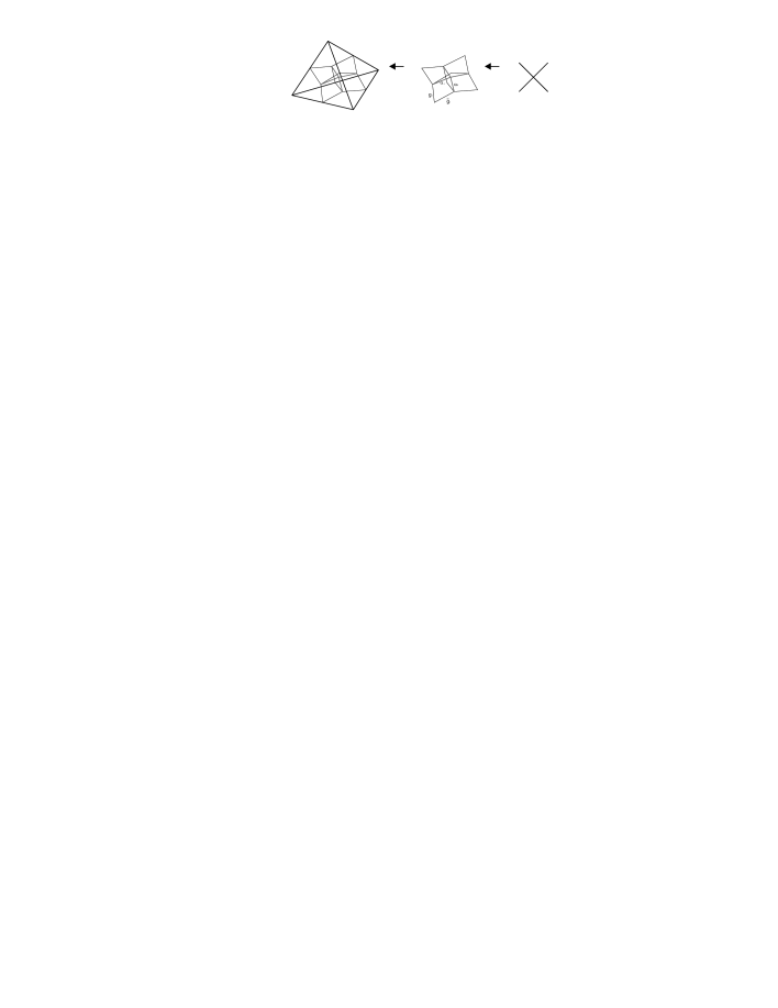
Figure 3: The pure gravity (Boulatov) tetrahedron.

The propagator $\mathcal{P}_{\phi}$ for the pure gravity sector represents geometrically the gluing of two tetrahedra obtained by identifying one triangle from each tetrahedron. The third term is the kinetic term for the coupled field. Its operator produces the propagator, $\mathcal{P}^{s}_{\psi}$, by inversion. The propagator is the identity on function space. It has an important role to play in the conservation of momentum as a particle travels from one tetrahedron to the next and we will discuss this in more detail in Section II.3, when we come to deal with generic Feynman diagrams generated by the perturbative expansion of the partition function.

The fourth term in the action $S_{gr+mat}^{int-2}$, with operator $\mathcal{V}^{s}_{2\psi}$, has two $\psi_{s}$ fields and two $\phi$ fields. This time two of the triangles have extra degrees of freedom related to matter. The arrangement of the gravity arguments once again gives it the form of a tetrahedron. In the operator (18), we have six $\delta$-functions over the holonomies around the wedges. Only four are forced to be flat; two have defects inserted. We wrote the amplitude for the particle degrees of freedom in a very simple form, however. This hides a more explicit description of the particle degrees of freedom and furthermore, it does not look like a CPR spin foam building block. We prove in Appendix E that the vertex term $S_{gr+mat}^{int-2}$ satisfies the following equality:

$$\begin{split}&\mu_{2}\int\prod^{6}_{i=1}dg_{i}\,du_{a}\;P_{\alpha_{1}}\psi_{s}(g_{1},g_{2},g_{3}u_{a}^{-1}hu_{a};u_{a})P_{\alpha_{2}}\psi_{s}(g_{4}u_{b}^{-1}h^{-1}u_{b},g_{3},g_{5};u_{a})P_{\alpha_{3}}\phi(g_{4},g_{2},g_{6})P_{\alpha_{4}}\phi(g_{6},g_{5},g_{1})\\ &=\mu_{2}\int\prod^{6}_{i=1}dg_{i}\,du_{a}\,du_{b}\;P_{\alpha_{1}}\psi_{s}(g_{1},g_{2},g_{3}u_{a}^{-1}hu_{a};u_{a})P_{\alpha_{2}}\psi_{s}(g_{4}u_{b}^{-1}h^{-1}u_{b},g_{3},g_{5};u_{b})P_{\alpha_{3}}\phi(g_{4},g_{2},g_{6})P_{\alpha_{4}}\phi(g_{6},g_{5},g_{1})\\ &\phantom{xxxxxxxxxxxxxxxxxxxxxxxxx}\times\delta(u_{a}^{-1}hu_{a}u_{b}^{-1}h^{-1}u_{b})\sum_{n_{a},n_{b}}D^{I}_{sn_{a}}(u_{a})D^{I}_{sn_{b}}(u_{b})\delta_{n_{a}n_{b}}.\end{split}$$ (21)

The amplitude coming from this vertex term lends itself to a much more explicit description of the particles’ degrees of freedom.

$$\begin{split}\mathcal{V}^{s}_{2\psi}=&\mu_{2}\int\prod_{i=1}^{4}d\alpha_{i}\;\delta(\bar{g}_{1}\alpha^{-1}_{4}\alpha_{1}g_{1}^{-1})\delta(\bar{g}_{2}\alpha^{-1}_{3}\alpha_{1}g_{2}^{-1})\delta(\bar{g}_{3}\alpha^{-1}_{2}\alpha_{1}u_{a}^{-1}hu_{a}g_{3}^{-1})\delta(\bar{g}_{4}\alpha^{-1}_{3}\alpha_{2}u_{b}^{-1}hu_{b}g_{4}^{-1})\\ &\hphantom{xxxxxxxxxxx}\times\delta(\bar{g}_{5}\alpha^{-1}_{4}\alpha_{2}g_{5}^{-1})\delta(\bar{g}_{6}\alpha^{-1}_{4}\alpha_{3}g_{6}^{-1})\delta(\alpha_{1}u_{a}^{-1}hu_{a}\alpha_{1}^{-1}\alpha_{2}u_{b}^{-1}h^{-1}u_{b}\alpha_{2}^{-1})\\ &\hphantom{xxxxxxxxxxxxxxxxxxx}\times\sum_{n_{a},n_{b}}D^{I}_{sn_{a}}(u_{a})D^{I}_{sn_{b}}(u_{b})\delta_{n_{a}n_{b}},\end{split}$$ (22)

where $I$ is any fixed representation of $\mathrm{SU}(2)$ such that $I-s\in\mathbb{N}$. We reiterate here that we label both particles, $a$ and $b$, by the same angular momentum $I$ and we do not sum over $I$. This stems from the fact that a bivalent particle interaction does not have any dependence on the total angular momenta and summing redundantly over them would result in infinities. In fact, we chose $I=s$ from now on. The defects we mentioned earlier are the momenta $u^{-1}hu$ of the particles associated to two edges of the tetrahedron. We illustrate them by the emboldened lines in FIG. 4, and denote them by $\daleth$, the particle graph. We denote the $\delta$-function, $\delta(\alpha_{1}u_{a}^{-1}hu_{a}\alpha_{1}^{-1}\alpha_{2}u_{b}^{-1}h^{-1}u_{b}\alpha_{2}^{-1})$ imposing explicit momentum conservation by a dotted curve encircling the vertex of the tetrahedron at which the two particles interact. This deals with the mass side of the particles’ degrees of freedom. But we must also account for their spin. The angular momenta, both the total and spin, reside on a dual particle graph $\daleth^{*}$. We draw this as the dashed line in FIG. 4. We label $\daleth^{*}$ by the matrix elements of the holonomy along the dashed line in the total angular momentum representation $I=s$. At the endpoints of the holonomies, we project the momenta of the particles down to the spin-s component:

$$D^{s}_{sn_{a}}(u_{a}\alpha_{1}^{-1})D^{s}_{sn_{b}}(u_{b}\alpha_{2}^{-1})$$ (23)

The bivalent interaction in $\daleth^{*}$ occurs at the dual vertex, where we place the intertwiner $\delta_{n_{a}n_{b}}$. We emphasise that the topological equivalence of the $\daleth$ and $\daleth^{*}$ is an imperative quality and determines in a large part how we define our model (see Appendix A).

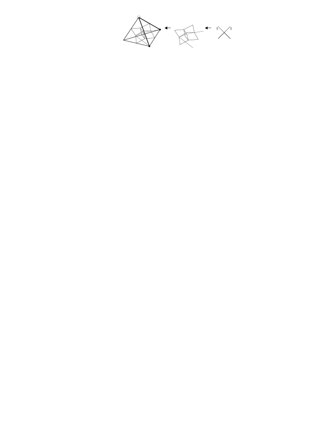
Figure 4: The tetrahedron with a bivalent particle interaction.

The vertex amplitude (22), as we have defined it is still not recognisable as a suitable building block for the amplitudes of the CPR model. This is due to the presence of the $\delta$-function enforcing explicit momentum conservation, and indeed the removal of this factor would supply us with a correct amplitude for one tetrahedron with two particles present. As a matter of fact the CPR spin foam amplitudes contain a type of implicit momentum conservation, which we explain precisely in Section III.1. Importantly for us, the presence of this $\delta$-function means that our amplitude satisfies an equation given pictorially in FIG. 5.

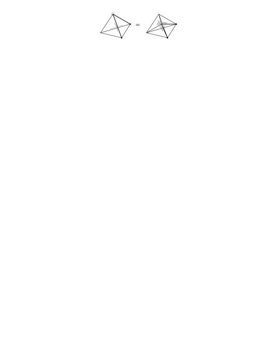
Figure 5: The 1-4 equality satisfied by the bivalent particle interaction term.

This graphically represents the following equation:

$$\begin{split}&\int\prod^{6}_{i=1}dg_{i}\,d\bar{g}_{i}\,du_{a}\,du_{b}\;\psi_{s}(g_{1},g_{2},g_{3};u_{a})\psi_{s}(g_{4},\bar{g}_{3},g_{5};u_{b})\phi(\bar{g}_{4},\bar{g}_{2},g_{6})\phi(\bar{g}_{6},\bar{g}_{5},\bar{g}_{1})\\ &\hphantom{xxxx}\times\mu_{2}\int\prod_{i=1}^{4}d\alpha_{i}\;\delta(\bar{g}_{1}\alpha^{-1}_{4}\alpha_{1}g_{1}^{-1})\delta(\bar{g}_{2}\alpha^{-1}_{3}\alpha_{1}g_{2}^{-1})\delta(\bar{g}_{3}\alpha^{-1}_{2}\alpha_{1}u_{a}^{-1}hu_{a}g_{3}^{-1})\\ &\hphantom{xxxxxxxxxxxxxxxxxxxx}\times\delta(\bar{g}_{4}\alpha^{-1}_{3}\alpha_{2}u_{b}^{-1}hu_{b}g_{4}^{-1})\delta(\bar{g}_{5}\alpha^{-1}_{4}\alpha_{2}g_{5}^{-1})\delta(\bar{g}_{6}\alpha^{-1}_{4}\alpha_{3}g_{6}^{-1})\\ &\hphantom{xxxxxxxxxxxxxxxxxxxxxxxxxxxxx}\times\delta(\alpha_{1}u_{a}^{-1}hu_{a}\alpha_{1}^{-1}\alpha_{2}u_{b}^{-1}h^{-1}u_{b}\alpha_{2}^{-1})\sum_{n_{a},n_{b}}D^{I}_{sn_{a}}(u_{a}\alpha_{1}^{-1})D^{I}_{sn_{b}}(u_{b}\alpha_{2}^{-1})\delta_{n_{a}n_{b}}\\ &=\int\prod^{6}_{i=1}dg_{i}\,d\bar{g}_{i}\,du_{a}\,du_{b}\int\prod_{i=1}^{4}d\alpha_{i}\prod_{j,k=1\;:\;j<k}^{4}d\gamma_{jk}\;\psi_{s}(g_{1},g_{2},g_{3};u_{a}\gamma_{14}\alpha_{1})\psi_{s}(g_{4},\bar{g}_{3},g_{5};u_{b}\gamma_{24}\alpha_{2})\phi(\bar{g}_{4},\bar{g}_{2},g_{6})\phi(\bar{g}_{6},\bar{g}_{5},\bar{g}_{1})\\ &\hphantom{xxxx}\times\mu_{2}\delta(\bar{g}_{1}\alpha^{-1}_{4}\gamma_{14}\alpha_{1}g_{1}^{-1})\delta(\bar{g}_{2}\alpha^{-1}_{3}\gamma_{13}\alpha_{1}g_{2}^{-1})\delta(\bar{g}_{3}\alpha^{-1}_{2}\gamma_{12}\alpha_{1}g_{3}^{-1})\delta(\bar{g}_{4}\alpha^{-1}_{3}\gamma_{23}\alpha_{2}g_{4}^{-1})\delta(\bar{g}_{5}\alpha^{-1}_{4}\gamma_{24}\alpha_{2}g_{5}^{-1})\delta(\bar{g}_{6}\alpha^{-1}_{4}\gamma_{34}\alpha_{3}g_{6}^{-1})\\ &\hphantom{xxxxxxxxxxxxxx}\times\delta(\gamma_{12}^{-1}\gamma_{24}^{-1}u_{a}^{-1}h^{-1}u_{a}\gamma_{14})\delta(\gamma_{13}^{-1}\gamma_{23}\gamma_{12})\delta(\gamma_{23}^{-1}\gamma_{34}^{-1}u_{b}^{-1}hu_{b}\gamma_{24})\delta(\gamma_{13}\gamma_{14}^{-1}\gamma_{34})\\ &\hphantom{xxxxxxxxxxxxxxxxxxxxx}\sum_{n_{a},n_{b}}D^{I}_{sn_{a}}(u_{a})D^{I}_{sn_{b}}(u_{b})\delta_{n_{a}n_{b}}.\end{split}$$ (24)

where the $\gamma$ variables refer to the holonomies along the newly introduced dual edges. In words, the left hand side is the amplitude $\mathcal{V}_{2\psi}$ as it occurs in (18). On the right hand side the tetrahedron has been replaced by four tetrahedra; this is the analogue of the 1-4 Pachner move of pure gravity in the case in which particles are present. The particle graph $\daleth$ has been ‘dragged’ into the interior and does not propagate along the original edges. Also we do not have explicit momentum conservation at the vertex of $\daleth$. So we see that our vertex operator is a building block for a CPR amplitude with a more refined triangulation. We prove this equality explicitly in Appendix C.

The fifth term $S_{gr+mat}^{int-3}$, with operator $\mathcal{V}^{s}_{3\psi}$, has a slightly different structure to $\mathcal{V}^{s}_{2\psi}$, except there are three triangles with extra degrees of freedom. As usual, it has a tetrahedral structure, but now three of the $\delta$-functions have defects indicative of particles on their associated edges. These form the particle graph $\daleth$. Moreover, there is explicit momentum conservation. For the angular momenta, the structure of the operator identifies a dual particle graph $\daleth^{*}$ with three edges and a trivalent intertwiner at the dual vertex. We mention also that the total angular momenta of the particles are different as a trivalent interaction depends on their individual values. We sum to get the most general amplitudes. The two graphs, $\daleth$ and $\daleth^{*}$, are again topologically equivalent. Finally, the explicit momentum conservation makes it again different at first sight from the CPR amplitude for three particles on one tetrahedron. However, the very same $\delta$-function is crucial for showing the equality of this amplitude to an amplitude of the CPR-type. This equality has the same form as that given in (24) but with an extra particle added. We represent it pictorially in FIG. 6.

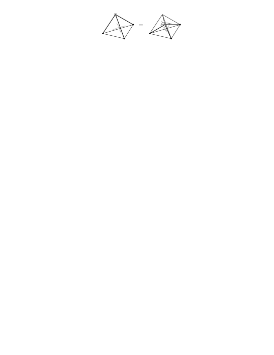
Figure 6: The equality satisfied by the trivalent particle interaction term.

The final term $S_{gr+mat}^{int-4}$, is that of the 4-valent particle interaction. Every vertex of a tetrahedron is trivalent, and therefore, to define a 4-valent particle interaction we must do it in a situation where there is a 4-valent vertex at least. Thus, it is clear that the vertex amplitude as we wrote it in (20) is hiding some information, that is, we have integrated out some variables to write it in a simpler form. But as in all these cases the vertex term $S_{gf+mat}^{int-4}$ satisfies an equality:

$$\begin{split}&\mu_{4}\int\prod^{6}_{i=1}dg_{i}\,du_{a}\,du_{b}\,du_{c}\,du_{d}\;\psi_{s}(g_{1},g_{2},g_{3}u_{a}^{-1}hu_{a};u_{a})\psi_{s}(g_{4}u_{b}^{-1}h^{-1}u_{b},g_{3},g_{5};u_{b})\psi_{s}(g_{2}u_{d}^{-1}hu_{d},g_{6},g_{4};u_{c})\\ &\phantom{xxxxxxxxxx}\times\psi_{s}(g_{6},g_{4},g_{2};u_{d})\delta(u_{a}^{-1}hu_{a}u_{b}^{-1}h^{-1}u_{b}u_{c}h^{-1}u_{c}u_{d}^{-1}hu_{d})\\ &\phantom{xxxxxxxxxx}\times\sum_{\begin{subarray}{c}I_{a},I_{b},I_{c},I_{d},\Lambda\\ n_{a},n_{b},n_{c},n_{d}\end{subarray}}D^{I_{a}}_{sn_{a}}(u_{a})D^{I_{b}}_{sn_{b}}(u_{b})D^{I_{c}}_{sn_{c}}(u_{c})D^{I_{d}}_{sn_{d}}(u_{d})\tilde{C}^{I_{a}\,I_{b}\,I_{c}\,I_{d}\,\Lambda}_{n_{a}n_{b}n_{c}n_{d}}\\ &=\mu_{4}\int\prod^{6}_{i=1}dg_{i}\,d\bar{g}_{i}\prod^{4}_{j=1}d\alpha_{j}\,du_{a}\,du_{b}\,du_{c}\,du_{d}\;\psi_{s}(g_{1},g_{2},g_{3};u_{a}\gamma_{14}\alpha_{1})\psi_{s}(g_{4},\bar{g}_{3},g_{5};u_{b}\gamma_{24}\alpha_{2})\psi_{s}(\bar{g}_{2},g_{6},\bar{g}_{4};u_{c}\alpha_{3})\\ &\phantom{xxxxxxxxxx}\times\psi_{s}(\bar{g}_{6},\bar{g}_{4},\bar{g}_{2};u_{d}\alpha_{4})\delta(\bar{g}_{1}\alpha^{-1}_{4}\gamma_{14}\alpha_{1}g_{1}^{-1})\delta(\bar{g}_{2}\alpha^{-1}_{3}\gamma_{13}\alpha_{1}g_{2}^{-1})\delta(\bar{g}_{3}\alpha^{-1}_{2}\gamma_{12}\alpha_{1}g_{3}^{-1})\\ &\phantom{xxxxxxxxxx}\times\delta(\bar{g}_{5}\alpha^{-1}_{4}\gamma_{24}\alpha_{2}g_{5}^{-1})\delta(\bar{g}_{4}\alpha^{-1}_{3}\gamma_{23}\alpha_{2}g_{4}^{-1})\delta(\bar{g}_{6}\alpha^{-1}_{4}\gamma_{34}\alpha_{3}g_{6}^{-1})\\ &\phantom{xxxxxxxxxx}\times\delta(\gamma_{12}^{-1}\gamma_{24}^{-1}u_{a}^{-1}h^{-1}u_{a}\gamma_{14})\delta(\gamma_{13}^{-1}u_{c}^{-1}hu_{c}\gamma_{23}\gamma_{12})\delta(\gamma_{23}^{-1}\gamma_{34}^{-1}u_{b}^{-1}hu_{b}\gamma_{24})\delta(\gamma_{13}\gamma_{14}^{-1}u_{d}^{-1}h^{-1}u_{d}\gamma_{34})\\ &\phantom{xxxxxxxxxx}\times\sum_{\begin{subarray}{c}I_{a},I_{b},I_{c},I_{d},\Lambda\\ n_{a},n_{b},n_{c},n_{d}\end{subarray}}D^{I_{a}}_{sn_{a}}(u_{a})D^{I_{b}}_{sn_{b}}(u_{b})D^{I_{c}}_{sn_{c}}(u_{c}\gamma_{34}^{-1})D^{I_{d}}_{sn_{d}}(u_{d})\tilde{C}^{I_{a}\,I_{b}\,I_{c}\,I_{d}\,\Lambda}_{n_{a}n_{b}n_{c}n_{d}},\end{split}$$ (25)

where we may prove this equality by following the same procedure as in Appendix C. We illustrate this new vertex term in FIG. 7.

Figure 7: The definition of the 4-valent particle interaction term.

We see that the vertex common to the four tetrahedra is 4-valent and so can play host to the interaction of the momenta. In the dual, any of the four dual vertices (by symmetry) will serve to facilitate the interaction of the angular momenta. We do not have any explicit momentum conservation here, and so we have a CPR building block. All further analysis follows that of the trivalent interaction term. For that reason we do not mention this term for the rest of the paper, but we state it here for completeness.

To conclude, we exhausted the possibilities for vertex terms. For example, although the vertex term $\mathcal{V}_{\psi}$ with one $\psi$ field allows the propagation of momentum along one edge of the tetrahedron, the spin degree of freedom has no such path in the dual as this requires two $\psi$ fields at least. Meanwhile, we cannot have more than 4-valent particle interactions in our model, as the dual to a triangulation is 4-valent, and we must preserve topological equivalence.

II.3 Quantum dynamics and Feynman amplitudes

We examine, in this section, the partition function and transition amplitudes. These define the quantum dynamical aspects of our theory. The dynamics has two facets: non-perturbative aspects and perturbative aspects. We do not investigate non-perturbative features as these are not well-understood even in the case of pure gravity (but see the important work of instantons ). In this work we focus on the perturbative features of our quantum theory. The first object of interest, which will receive most attention, is the partition function, defined in perturbative expansion as:

$$\begin{split}Z=&\int\mathcal{D}\psi_{s}\mathcal{D}\phi\;e^{-S[\phi,\psi_{s}]},\\ =&\sum_{\Gamma}\frac{\lambda^{v_{0}[\Gamma]}\mu_{2}^{v_{2}[\Gamma]}\mu_{3}^{v_{3}[\Gamma]}}{sym[\Gamma]}Z[\Gamma],\end{split}$$ (26)

We denote each term in the expansion by a Feynman diagram $\Gamma$, and each $\Gamma$ has an amplitude $Z[\Gamma]$. Moreover, $sym[\Gamma]$ is the symmetry factor of the graph, $v_{0}[\Gamma]$ is the number of Boulatov tetrahedra, $v_{2}[\Gamma]$ is the number of tetrahedra with a bivalent particle interaction and $v_{3}[\Gamma]$ is the number of tetrahedra with a trivalent particle interaction. We may construct these terms in the summation with the aid of a graphical calculus which we have been developing over the course of the paper. We have a 4-valent graph with two types of line, full and dashed, and three types of vertex: four full lines incident, two full and two dashed, and one full and three dashed. Then we label them as below:

$$\mathcal{P}_{\phi}(g_{i},\bar{g_{i}})$$

$$\mathcal{P}^{s}_{\psi}(g_{i},\bar{g_{i}},u,\bar{u})$$

$$\int\prod_{i=1}^{6}dg_{i}\,d\bar{g}_{i}\;\mathcal{V}_{\phi}(g_{i},\bar{g_{i}})$$

$$\int\prod_{i=1}^{6}dg_{i}\,d\bar{g}_{i}\,du_{a}\,du_{b}\;\mathcal{V}^{s}_{2\psi}(g_{i},\bar{g_{i}},u_{a},u_{b})$$

$$\int\prod_{i=1}^{6}dg_{i}\,d\bar{g}_{i}\,du_{a}\,du_{b}\,du_{c}\;\mathcal{V}^{s}_{3\psi}(g_{i},\bar{g_{i}},u_{a},u_{b},u_{c})$$

Products of these form the Feynman graph and its structure is dual to the structure of a triangulation. This is just conventional Feynmanology for a path integral formulation of a field theory.

We can express the operators using strand diagrams. They are an intermediary calculus between the utter minimalism of the Feynman graphs and the more complicated formalism of the fully reconstruction of the triangulation. To each pure gravity line we associate three strands, and to each coupled line four strands. We label the endpoints of the solid strands by the $g$ arguments, and the endpoints of the dotted strand by the momentum of the particle $u$. We label the solid edges themselves by the $\delta$-function over the holonomy which contains the $g$ arguments of its two endpoints, while the dotted strands are labelled by the angular momentum amplitude. Once vertices are glued using the propagators, the solid strands form loops which are the plaquettes dual to an edge of the triangulation and the dotted strands form the dual particle graph $\daleth^{*}$.

We have yet to show that each term $Z[\Gamma]$ is a spin foam amplitude. A generic Feynman graph $\Gamma$ in the partition function is a closed 4-valent graph labelled as above. The integration over $g$ and $u$ variables glues the vertex amplitudes, the propagators being essentially identity operators. There are basically three interesting subsets of diagrams that occur:

$$\begin{array}[]{cccc}v_{0}\neq 0,&\quad\quad v_{2}=0,&\quad\quad v_{3}=0,&\quad\quad\textrm{pure gravity,}\\ v_{0}\neq 0,&\quad\quad v_{2}\neq 0,&\quad\quad v_{3}=0,&\quad\quad\textrm{non interacting particles coupled to gravity,}\\ v_{0}\neq 0,&\quad\quad v_{2}\neq 0,&\quad\quad v_{3}\neq 0,&\quad\quad\textrm{interacting particles coupled to gravity.}\end{array}$$

Consider the first scenario and the simplest. These are the diagrams occurring in Boulatov field theory for pure gravity. Note that each of the vertices of the Feynman graph is dual to a tetrahedron and thus the integration of $g$ variables glues tetrahedra together to form a triangulation. To understand the amplitudes we move to the dual picture where the aforementioned integration glues wedges together to form faces each dual to an edge of the triangulation. Therefore, we are left with a $\delta$-function for the holonomy around each face of the dual which enforces the flatness condition on the curvature. This is exactly the Ponzano-Regge spin foam amplitude for pure 3d Riemannian quantum gravity laurentPRI .

We now approach the more delicate task of constructing diagrams including matter in their amplitudes. The form of the amplitudes can be extrapolated from the gluing of two vertices with bivalent particle interactions. The contruction works analogously in the case of 3-valent and 4-valent particle interactions, so we do not discuss these other cases in detail. The propagator glues the tetrahedra together at a face and ensures the conservation of momentum explicitly at the vertex of the triangulation where the segments of the particle graphs meet. It also ensures the conservation of spin in the dual particles graphs explicitly. We give this visually in FIG. 8.

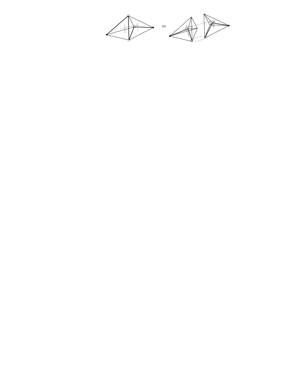
Figure 8: The gluing of two coupled tetrahedra.

This can be written as a CPR amplitude very easily after some rearrangement. First we use the 1-4 equality to remove the signs of explicit momentum conservation at two of the vertices (see Appendix C). This is given in FIG. 8 also. We remove the final explicit $\delta$-function in two steps. The original shared face of the triangulation is now shared by two smaller tetrahedra. These are drawn on the lhs of FIG. 9. Each of the tetrahedra has a particle on an edge. We know we can use the 1-4 equality to remove explicit momentum conservation when the particles are in the same tetrahedron. Fortunately, the 2-3 Pachner equality is satisfied by these two tetrahedra when particles are present. We prove this in Appendix D and draw it here in FIG. 9. Now that the two particles are in the same tetrahedron, a final 1-4 equality can be invoked. We arrive at an amplitude that has no explicit signs of momentum conservation and is a CPR amplitude.

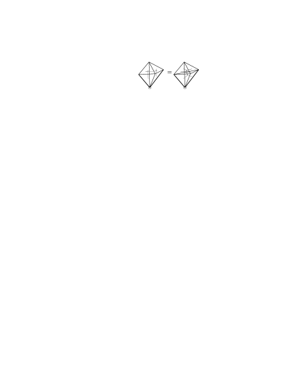
Figure 9: The 2-3 equality satisfied by the coupled tetrahedra.

In effect the amplitude we see on gluing two of our vertices together is the coarse graining of a CPR spin foam amplitude for a finer triangulation, i.e. with some of the arguments integrated out. The above reorganisation is indicative of the procedure when two coupled tetrahedra are glued together, and gives us the insight necessary to chronicle the form of a generic Feynman graph for matter coupled to gravity. For a normal edge of the triangulation we get the usual curvature flatness constraint. For an edge of the particle graph $\daleth$, we find that there is a defect in the curvature equal to the momentum of the particle. For the dual particle graph $\daleth^{*}$, we labelled it by the matrix elements of its holonomy in the total angular momentum interspersed with spin projections, one for each particle, and angular momentum intertwiners one for each particle interaction. This is exactly a CPR spin foam amplitude.

The next object is a definition of the transition amplitudes. fortunately, we have done the background work on this already so we can proceed and state it as the ‘two point’ or more precisely, ‘two net’ function:

$$<\theta_{1}|\theta_{2}>=\int\mathcal{D}\psi_{s}\mathcal{D}\phi\;\theta_{1}[\phi,\psi_{s}]\theta_{2}[\phi,\psi_{s}]e^{-S[\phi,\psi_{s}]}$$ (27)

where $\theta_{1}$ and $\theta_{2}$ are the boundary states, i.e. products of the Boulatov and coupled fields based on open spin networks. We give a portion of a typical boundary state in FIG. 10.

Figure 10: Portion of a typical boundary state.

FIG. 10 evaluates to

$$\dots\Phi^{j_{1}\;\;j_{2}\;\;j_{3}}_{m_{1}m_{2}m_{3}}\Psi^{j_{3}\;\;j_{4}\;\;j_{5}\;\,I_{a}\;\Lambda_{a}}_{m_{3}m_{4}m_{5}s}\Psi^{j_{6}\;\;j_{5}\;\;j_{7}\;\,I_{b}\;\Lambda_{b}}_{m_{6}m_{5}m_{7}s}\dots$$ (28)

with repeated indices summed over. This concludes our definition of the model.

III Features of the new model - extended discussion

III.1 Feynman Amplitudes

In Section II we detailed the definition of our model but we postponed almost all explanation of our reasons for the particular form we chose. The model in question has many intriguing characteristics which deserve further clarification since they play non-obvious roles in ensuring the faultless realisation of the Feynman amplitudes as CPR spin foam amplitudes. Among these, two are most notable: the amplitudes are defined with explicit momentum conservation at every vertex of $\daleth$; also, we do not impose permutation invariance in the coupled field.

Before we elucidate our reasoning we give some background information on the CPR amplitudes that is especially relevant here. The topic is the implicit momentum conservation contained in the CPR spin foam model. For sake of completeness, we start from the very beginning. Classically, first order 3d Riemannian gravity is a BF theory. The curvature $F$ satisfies a Bianchi identity, $dF=0$, and as $dF$ is a 3-form it couples to volumes. Upon discretising the manifold and quantising the theory, the continuum Bianchi identity is lost, understandably, but a discrete remnant survives. We describe this by considering a vertex of the triangulation $\Delta$, and all the edges emanating from it. Each of these edges is dual to a face of the spin foam and therefore has a holonomy associated to it. These faces close to form a 3-ball around the vertex and thus identify the boundary of a volume. The discrete version of the Bianchi identity states that there exists an ordered product of these holonomies which evaluates to the unit element laurentPRI . For pure gravity, since the very quantum amplitude enforces the flatness of the holonomy this identity gives us no more restrictions on the dynamics of the theory. Now, consider a vertex where $n$ of the edges have particles propagating along them. The amplitude for these edges is a $\delta$-function over the holonomy with a momentum defect. Thus, the holonomy is forced to be the momentum of the particle and the product of holonomies in the Bianchi Identity reduces to a product over the momenta incident at the vertex. Thus, we have implicit overall momentum conservation. This is not sufficient for our purposes, however. Unlike the spin foam quantisation, where one has an explicit knowledge of the discretisation structure, i.e. the triangulation $\Delta$ and the dual spin foam $\Delta^{*}$, before one begins, and one has hands-on control over the particle graphs, $\daleth$ and $\daleth^{*}$ and how one labels them, i.e. what are the variables living on them, the group field theory does not allow such freedom and control. We generate the spin foams, after all, as Feynman graphs and we only know the action to start with. To illustrate the way momentum conservation is realised in our model and the topological equivalence between $\daleth$ and $\daleth^{*}$ is mantained, in spite of this lack of control, we develop two examples.

As our first case, since in our Feynman expansion we generate all possible graphs given the Feynman rules, one possibility is that in FIG. 11. These tetrahedra have one vertex in common and it happens to be the one where both of them have a bivalent particle interaction in $\daleth$. Implicit momentum conservation here would imply that all the four momenta incident to the vertex would sum up to zero, with orientation taken into account, but this would allow for the identification of a 4-valent matter interaction vertex on $\daleth$, instead of two bivalent ones. This disagrees with the two bivalent particle interactions in $\daleth^{*}$, and so we would not have a CPR amplitude, due to the breaking of the equivalence of $\daleth$ and $\daleth^{*}$. In other words, the implicit momentum conservation that we know is present in the Feynman amplitudes is not enough to guarantee the well-posedness of the model. Since we have explicit momentum conservation, this scenario does not arise and we have the correct particle graph structure. It is gratifying also to see that the introduction of explicit momentum conservation means that we can separate the two particle interactions by the ‘dragging’ procedure of the 1-4 equality. In this way the ambiguous situation discussed above is simply removed, as $\daleth$ and $\daleth^{*}$ have now manifestly the same structure. This confirms the more fundamental nature of the dual particle graph $\daleth*$ (at least in our model) and that ambiguous configurations arise only as a result of ‘pathological’ embeddings of the dual particle graph in the triangulation, or equivalently, as a result of coarse graining of the same triangulation, performed by means of Pachner moves.

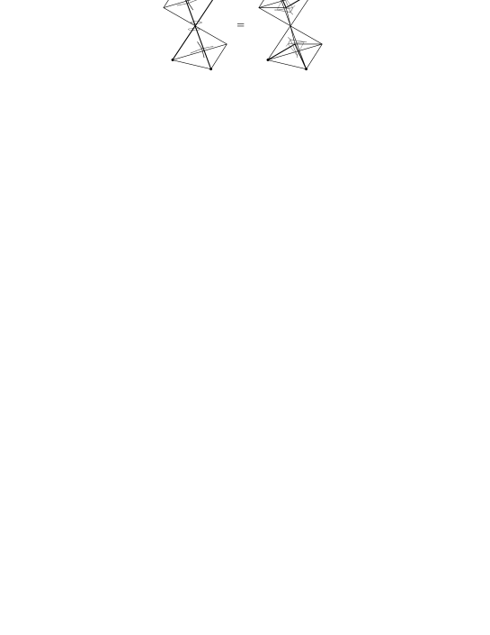
Figure 11: Two tetrahedra sharing the same vertex (both having a bivalent interaction there).

The second example displays a different problem and its solution. Another possibility in a Feynman diagram is that we generate two tetrahedra that share an edge which happens to be an edge where both tetrahedra have a particle propagating. This could be at first sight interpreted indeed as the presence of two particles propagating along the same edge of the triangulation, and the implicit momentum conservation would be compatible with this interpretation. This type of configuration does not occur in the CPR amplitudes of laurentPRI , and is again a pathological result of inappropriate coarse graining of the triangulation. Their pathological nature is clear if we recall that we interpret the particle graphs as Feynman graphs of a matter field theory coupled to gravity, so that lines should represent one-particle propagation, and that the CPR amplitudes reduce indeed in the effective limit to Feynman diagrams of a non-commutative quantum field theory, so they lie within a larger multiparticle structure. We neither need nor want multiple particles on an edge. With 1-4 equality, i.e. by application of a Pachner move on the triangulation labelled by particle degrees of freedom, this pathology can be overcome and the particle graph ‘resolved’ into a physically equivalent one (because it has equal amplitude) that shows no ambiguous ‘multi-particle’ appearance.

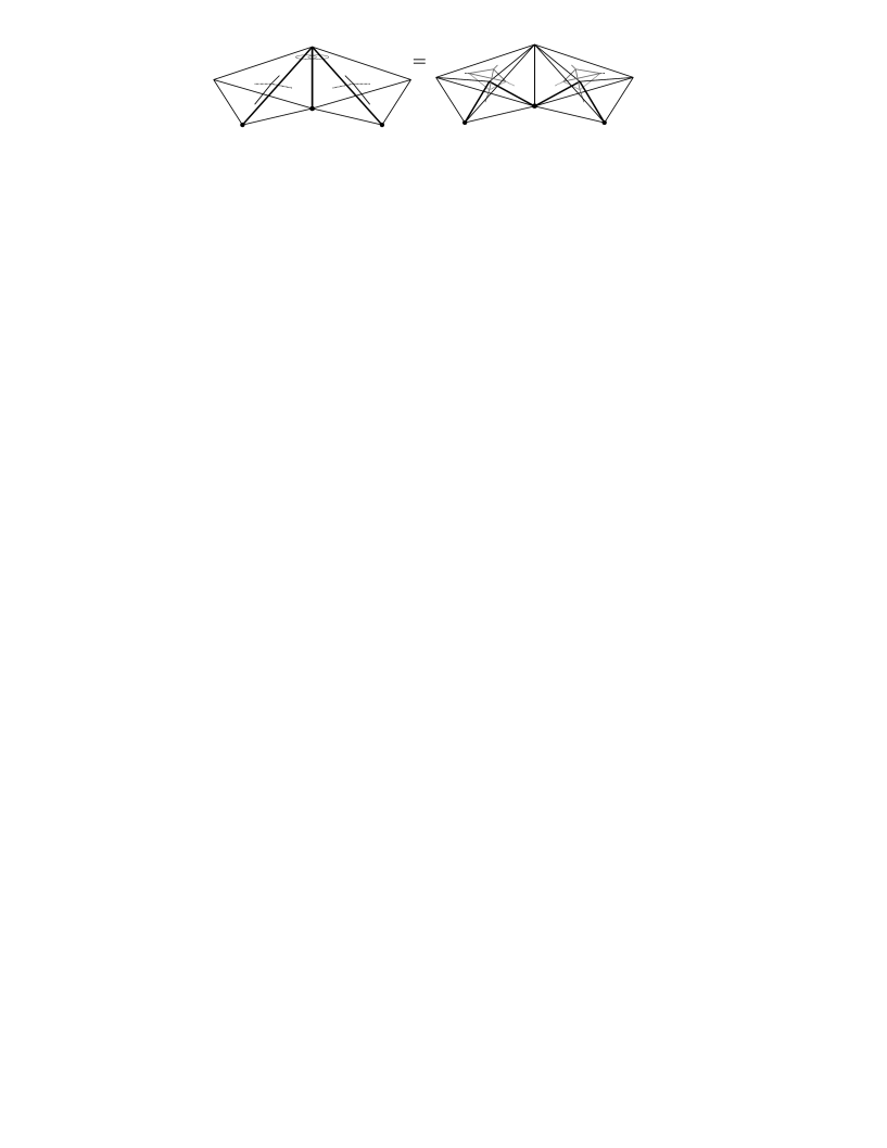
Figure 12: Two tetrahedra sharing the same edge (both contributing a particle there).

Again, the crucial point is the topological equivalence of $\daleth$ and $\daleth^{*}$, so let us discuss this a bit more. In the spin foam context where we have complete control of the variables it is natural to consider the particle graph residing in $\Delta$ as more fundamental and the particle graph $\daleth^{*}$ in $\Delta^{*}$ as a framing of $\daleth$ in the dual which gives a consistent picture of how the angular momenta propagates. This is not, however, the way we picture things when dealing with the amplitudes generated by the GFT, even though they are the same as those of the CPR spin foams. We perform a conceptual shift. This begins with the proposal of a new field to describe matter coupled to gravity. We see that this helps create the sense of the particle graph $\daleth^{*}$ in $\Delta^{*}$ as our initial concept. In other words, our Feynman expansion creates first a particle graph $\daleth^{*}$ alongside the dual complex from which the triangulation is reconstructed; from this, taking into account the way the variables associated with this dual graph $\daleth*$ are coupled with the gravity degrees of freedom, one has to reconstruct a particle graph $\daleth$, lying on the triangulation itself. In fact, the positioning of the momentum in the field gives rise to the particle graph $\daleth$ when we reconstruct $\Delta$ and all our efforts have been to ensure that $\daleth$ is topologically equivalent to $\daleth^{*}$. Thus we can consider $\daleth$ as an embedding of $\daleth^{*}$ into the triangulation. It is then easy to see that topological equivalence forces us not to impose the usual permutation invariance of pure gravity on the coupled field. To exemplify the type of problematic configurations that arise were we to require permutation invariance in the coupled field, consider the structure obtained by gluing two tetrahedra as in FIG. 13. This is similar to the gluing of two tetrahedra in FIG. 8. The edges on the shared face of one tetrahedron, however, are permuted cyclically with respect to the edges of the other.

Figure 13: A configuration coming from requiring permutation invariance.

The particle graph $\daleth$ no longer describes the continuous propagation of a particle, even though momentum is conserved. Topological equivalence is lost.

We should also discuss to what extent our model encompasses the CPR spin foam amplitudes in all their generality. For spinning particles, topological equivalence requires that the particle graphs of the CPR spin foams have at most 4-valent interactions. So, no generality is lost there. However, if spinless particles are dealt with as a special case of our more general formalism, the same restriction would apply to them, while in the spin foam amplitudes of the CPR model no limit on the order of interaction for a scalar field was imposed. Thus at first sight it seems that some generality may be lost; it is not easy on the other hand to confirm this impression nor to disprove it, given that we are able to relate certain graphs arising in our model using Pachner moves, and that this is possible also in the CPR amplitudes; by doing so higher valent interaction vertices for scalar particles can be resolved into lower valent ones, as well as the opposite. Furthermore, we note that it is possible as well to generalise our model to one that produces higher valent vertices even for spinning particles/fields: we would have to generalise the discretisation structures arising from the perturbative expansion, and in particular those structures we reconstruct from Feynman vertices from tetrahedra to polyhedra, as the dual vertex would then have a higher number of incident dual edges. In any case we see that a model with a restriction on interaction vertices to be 4-valent would thus look more fundamental in nature.

III.2 Many particle species

To this point, our model incorporated just one species of particle with a fixed mass and spin, albeit arbitrary. We extend our model here to include many species of particle. This is done easily at the dynamical level by adding new kinetic and vertex terms to the action, with a similar structure to those already present. We write down the terms in a new shorthand notation, that should, however, be of no difficult to interpret. In this notation, our original action is

$$S[\phi,\psi_{s,m}]=S_{\phi\phi}+S_{\phi\phi\phi\phi}+S_{\psi_{s,m}\psi_{s,m}}+S_{\psi_{s,m}\psi_{s,m}\phi\phi}+S_{\psi_{s,m}\psi_{s,m}\psi_{s,m}\phi}.$$ (29)

The new terms are of such a similar form that we can extend as follows:

$$S[\phi,\psi_{s,m},\psi_{\bar{s},\bar{m}}]=S[\phi,\psi_{s,m}]+S_{\psi_{\bar{s},\bar{m}}\psi_{\bar{s},\bar{m}}}+S_{\psi_{\bar{s},\bar{m}}\psi_{\bar{s},\bar{m}}\phi\phi}+S_{\psi_{\bar{s},\bar{m}}\psi_{\bar{s},\bar{m}}\psi_{\bar{s},\bar{m}}\phi}+S_{\psi_{\bar{s},\bar{m}}\psi_{s,m}\psi_{s,m}\phi}+S_{\psi_{\bar{s},\bar{m}}\psi_{\bar{s},\bar{m}}\psi_{s,m}\phi}$$ (30)

The first three are just a replica of the terms given for the $(s,m)$ particle earlier. The final two allow for interaction between the two species. Further generalisations follow the same path.

We do not specify the Feynman rules for the partition function and transition amplitude explicitly but we describe the generic structure of the diagrams that occur in the partition function, and their particle graphs. Since the action contains the action of 13, we get all the diagrams that we had before. Furthermore, there is a subset of terms for the $(\bar{s},\bar{m})$ particles coupled to gravity that are a direct copy of the terms for $(s,m)$. This means we get a copy of the $(s,m)$ particle diagrams for the $(\bar{s},\bar{m})$ particles. Finally, we get the diagrams charting the interaction between the two species. We give a portion of a typical example in FIG. 14.

Figure 14: A generic multi-species Feynman diagram.

Kinematically, we can have boundary states containing particles of both species, $\theta(\phi,\psi_{s,m},\psi_{\bar{s},\bar{m}})$. These have the same form as before. They are based on open trivalent graphs where some of the particle vertices are labelled by the $\psi_{\bar{s},\bar{m}}$ and some by $\psi_{s,m}$. Thus, there exist non-zero transition amplitudes between multi-species, multi-particle states.

III.3 DSU(2) structures and Lorentz deformation

Let us discuss briefly the role of non-commutative and specifically $DSU(2)$ structures in our model. It is known that quantum point particles in 3d manifest a symmetry under a quantum group deformation of the Poincaré group, i.e. the non-compact double of $SU(2)$, $DSU(2)$ matschullwelling ; laurentPRI ; laurentPRII ; jurleelau , and that this deformed symmetry structure can be identified clearly, made explicit and put to use in the CPR spin foam model laurentPRI ; laurentPRII and in the effective field theory for scalar matter fields derived from it laurentPRIII . Therefore, one may wonder what role $DSU(2)$ structures play in our GFT model, and maybe expect that a correct group field theory derivation of the CPR spin foam model should be based directly on such $DSU(2)$ structures instead of using only the $SU(2)$ group elements and representations as is the case for our model. We think this is not the case and the evidence that can be gathered from the literature suggests that, while a $DSU(2)$ symmetry is likely to be implicitly present in our model, a purely $SU(2)$-based formulation of 3d gravity coupled to matter at the group field theory level is in our opinion not only sensible, but arguably the most natural way to proceed.

The main reason for this is that not only the expression of the CPR spin foam model, but also both its known derivations from covariant path integral methods in a discrete setting laurentPRI and from canonical Hamiltonian methods in the continuum KarimAlex , make use of elements and representations of $SU(2)$, and of its inhomogeneous counterpart (i.e. the Poincaré group), only. In laurentPRI , the authors started with a discretisation of the continuum action for 3d gravity coupled to point particles, which is invariant under local $SU(2)$ transformations only, and with the particles labelled by Poincaré representations. They then derived, using spin foam techniques, the CPR model where, as explained in detail in Appendix A, the modified amplitudes are functions of $SU(2)$ group elements and group representations only. Also, boundary data for the partition function are ordinary open spin networks again based on $SU(2)$. Analogously, one can start from a conventional definition of canonical kinematical states for matter coupled to quantum gravity in terms of open $SU(2)$ spin networks and Poincaré representations. Then, one can define KarimAlex and explicitly construct, using a rigorous discretisation and application of usual loop quantum gravity methods, a projection operator onto solutions of the Hamiltonian constraint and a physical scalar product for canonical states given again by the CPR spin foam model. The interesting point is that in spite of this more conventional-looking expression of the partition function, one can identify laurentPRI a non-trivial braiding for the particles. This results from the action of the braiding matrix of the quantum group $DSU(2)$. Also, the same partition function, for a given coupled Feynman graph for matter fields, can be re-expressed laurentPRII as the evaluation of a colored chain mail link based again on the same quantum group. These results make clear that quantum group symmetries are a result of the quantum dynamics of gravity coupled to particles and not of the kinematics behind it. But these results also make clear that the use of un-deformed $SU(2)$ structures and of related spin foam techniques for describing these quantum dynamics is fully compatible with the presence of deformed symmetries for matter fields and with the use of quantum group techniques for the evaluation of the same physical quantities.

Let us also stress, in support of this conclusion, that the equivalence of the Ponzano-Regge spin foam model, expressed and derived only using $SU(2)$ structures, with a quantum group evaluation of a chain mail link based on $DSU(2)$ is true also in the simpler case of pure gravity with no matter coupling laurentPRII . As for the group field theory derivation of such a model, it is well known that this is given by the Boulatov group field theory boulatov , i.e. by a field theory over an ordinary $SU(2)$-based group manifold, in spite of this alternative reformulation based on $DSU(2)$.

There is more. The most striking appearance of non-commutative structures from the CPR model is in our opinion the derivation of an effective non-commutative field theory for a scalar field encoding the quantum gravity corrections laurentPRIII . Here, it is clear that quantum gravity dynamics is responsible for the deformation of ordinary field theory to a non-commutative one. Again, however, in momentum space the resulting field theory is just one based on an $SU(2)$ group manifold. The non-commutative structure of spacetime emerges only after harmonic analysis, due to the curvature of momentum space laurentPRIII . The $DSU(2)$ symmetry manifests itself not at the level of the action but when considering multiparticle states, their non-trivial braiding and their modified scattering laws. It is a field theory of this type, based on the $SU(2)$ group manifold, that we expect to obtain from a group field theory action, at an effective level, after suitable integration of the gravity degrees of freedom.

In spite of all this evidence for the adequacy of using only $SU(2)$ structures for constructing a group field theory describing 3d quantum gravity coupled to matter fields, one may still want to look for an alternative formulation that makes explicit use of the quantum group $DSU(2)$; perhaps for the need for greater simplicity or simply because of the beautiful mathematical structures this would bring into play. This would certainly be an interesting and fascinating project, but the results of kirillgft lead one to approach this issue with greater caution. As already mentioned, in fact, in kirillgft the author studies the straightforward generalisation of the Boulatov model to the case of $DSU(2)$, and the whole construction proceeds beautifully and rigorously, but the resulting model does not admit any clear interpretation in terms of matter fields coupled to gravity (and definitely does not reproduce the CPR spin foam model) that can be considered as a sensible coupling of 3d quantum gravity with Feynman graphs for matter fields. This suggests that something more elaborate may be needed. We leave this for future work.

III.4 Generalised model with variable mass and spin

An interesting generalisation which has received some attention kirillgft (and we expect it to receive more shortly karim ) is to relax our constraints on the mass and spin completely. To state things explicitly, we integrate over all masses and sum over every spin. From one base, we could regard this as allowing for every possible spin given a certain mass. Or from the other, for a given spin every mass is possible. Thus there is an infinite number of species of particles. We give the action as:

$$\begin{split}S[\phi,\psi]=&\;\frac{1}{2}\int\prod^{3}_{i=1}dg_{i}\;P_{\alpha}\phi(g_{1},g_{2},g_{3})P_{\bar{\alpha}}\phi(g_{1},g_{2},g_{3})\\ &+\frac{\lambda}{4!}\int\prod^{6}_{i=1}dg_{i}\;P_{\alpha_{1}}\phi(g_{1},g_{2},g_{3})P_{\alpha_{2}}\phi(g_{3},g_{5},g_{4})P_{\alpha_{3}}\phi(g_{4},g_{2},g_{6})P_{\alpha_{4}}\phi(g_{6},g_{5},g_{1})\\ &+\frac{1}{2}\int dg_{i}du\;\sum_{s}P_{\alpha}\psi_{s}(g_{1},g_{2},g_{3};u)P_{\bar{\alpha}}\psi_{s}(g_{1},g_{2},g_{3};u)\\ &+\mu_{2}\int\prod^{6}_{i=1}dg_{i}\,du_{a}\int dh\sum_{s}P_{\alpha_{1}}\psi_{s}(g_{1},g_{2},g_{3}u_{a}^{-1}hu_{a};u_{a})P_{\alpha_{2}}\psi_{s}(g_{4}u_{a}^{-1}h^{-1}u_{a},g_{3},g_{5};u_{a})\\ &\phantom{xxxxxxxxxx}\times P_{\alpha_{3}}\phi(g_{4},g_{2},g_{6})P_{\alpha_{4}}\phi(g_{6},g_{5},g_{1})\\ &+\mu_{3}\int\prod^{6}_{i=1}dg_{i}\,du_{a}\,du_{b}\,du_{c}\;\int dh_{a}\,dh_{b}\,dh_{c}\sum_{s_{a},s_{b},s_{c}}P_{\alpha_{1}}\psi_{s_{a}}(g_{1},g_{2},g_{3}u_{a}^{-1}h_{a}u_{a};u_{a})P_{\alpha_{2}}\psi_{s_{b}}(g_{4}u_{b}^{-1}h_{b}^{-1}u_{b},g_{3},g_{5};u_{b})\\ &\phantom{xxxxxxxxxx}\times P_{\alpha_{3}}\psi_{s_{c}}(g_{6},g_{4},g_{2}u_{c}^{-1}h_{c}u_{c};u_{c})P_{\alpha_{4}}\phi(g_{6},g_{5},g_{1})\delta(u_{a}^{-1}h_{a}u_{a}u_{b}^{-1}h_{b}^{-1}u_{b}u_{c}^{-1}h_{c}u_{c})\\ &\phantom{xxxxxxxxxxxxxxxxxxxx}\times\sum_{\begin{subarray}{c}I_{a},I_{b},I_{c}\\ n_{a},n_{b},n_{c}\end{subarray}}D^{I_{a}}_{s_{a}n_{a}}(u_{a})D^{I_{b}}_{s_{b}n_{b}}(u_{b})D^{I_{c}}_{s_{c}n_{c}}(u_{c})C^{I_{a}\,I_{b}\,I_{c}}_{n_{a}n_{b}n_{c}}\end{split}$$ (31)

We should note that in the second vertex term, that is the vertex with a bivalent particle interaction, we have written the two particles with the same mass and spin because even if we allowed them to differ, the relations above would force the amplitude to be zero except when they coincided, due to momentum conservation. On the boundary, we retain states with fixed mass and spin for any one particle, and one can obviously have more than one species of particle in a kinematic state. This is what we measure in practice, i.e. in real life situations, and we wish to retain some sort of touch with possible future experiment. This loosening of restrictions affects the amplitudes, of course. More strikingly, it alters the effective limit of the theory, and indeed the abelian limit of the theory where one recovers usually ordinary quantum field theory. This group field theory reduces to analogous theories but with the sum over all masses and spins maintained, thus to field theories with variable mass and spin; while we are aware of past work on quantum field theories with indefinite mass (see for example feynman ; hostler ), we do not recall a similar generalisation for the spin degrees of freedom.

III.5 Reduced model - scalar fields

Let us consider the limiting case in which both the spin of the particle and its total angular momentum go to zero, i.e. the case of 3d quantum gravity coupled to a single scalar field with no angular momentum. In us , a model was proposed to describe such happenstance, based on a formalism, a type of field and relative action that are quite different from the ones we use in the corresponding limit of our present model. However, they produce, modulo multiplicative factors, the same Feynman amplitudes. It is interesting then to understand the exact relation between these two models. We converge on a reconciliation first from the side of our new model. The action for scalar particles reduces to:

$$\begin{split}S[\phi,\psi]=&\;\frac{1}{2}\int\prod^{3}_{i=1}dg_{i}\;P_{\alpha}\phi(g_{1},g_{2},g_{3})P_{\bar{\alpha}}\phi(g_{1},g_{2},g_{3})\\ &+\frac{\lambda}{4!}\int\prod^{6}_{i=1}dg_{i}\;P_{\alpha_{1}}\phi(g_{1},g_{2},g_{3})P_{\alpha_{2}}\phi(g_{3},g_{5},g_{4})P_{\alpha_{3}}\phi(g_{4},g_{2},g_{6})P_{\alpha_{4}}\phi(g_{6},g_{5},g_{1})\\ &+\frac{1}{2}\int dg_{i}du\;P_{\alpha}\psi_{0}(g_{1},g_{2},g_{3};u)P_{\bar{\alpha}}\psi_{0}(g_{1},g_{2},g_{3};u)\\ &+\mu_{2}\int\prod^{6}_{i=1}dg_{i}\,du_{a}\;P_{\alpha_{1}}\psi_{0}(g_{1},g_{2},g_{3}u_{a}^{-1}hu_{a};u_{a})P_{\alpha_{2}}\psi_{0}(g_{4}u_{a}^{-1}h^{-1}u_{a},g_{3},g_{5};u_{a})P_{\alpha_{3}}\phi(g_{4},g_{2},g_{6})P_{\alpha_{4}}\phi(g_{6},g_{5},g_{1})\\ &+\mu_{3}\int\prod^{6}_{i=1}dg_{i}\,du_{a}\,du_{b}\,du_{c}\;P_{\alpha_{1}}\psi_{0}(g_{1},g_{2},g_{3}u_{a}^{-1}hu_{a};u_{a})P_{\alpha_{2}}\psi_{0}(g_{4}u_{b}^{-1}h^{-1}u_{b},g_{3},g_{5};u_{b})P_{\alpha_{3}}\psi_{0}(g_{6},g_{4},g_{2}u_{c}^{-1}hu_{c};u_{c})\\ &\phantom{xxxxxxxxxx}\times P_{\alpha_{4}}\phi(g_{6},g_{5},g_{1})\delta(u_{a}^{-1}hu_{a}u_{b}^{-1}h^{-1}u_{b}u_{c}^{-1}hu_{c})\end{split}$$ (32)

We have no longer spin and angular momentum degrees of freedom identifying a dual particle graph $\daleth^{*}$, we are only interested in the particle graph $\daleth$, where we still have explicit momentum conservation, and thus have at most trivalent particle interactions (as we have not included 4-valent interaction terms in the above action). No restriction comes then from the need to have topological equivalence of $\daleth$ and $\daleth^{*}$. The above action produces, in perturbative expansion, the CPR amplitudes for scalar particles. The presence of explicit momentum conservation, i.e. of extra deltas relating the $u$ variables, allows for the use of Pachner moves to resolve pathological multiparticle-like configurations (in the sense explained above). If we go one step further and remove explicit momentum conservation, we recover a model in which multiple particles reside on some edges and we have arbitrary valence interactions in the particle graph $\daleth$. These are not CPR amplitudes, and correspond to the amplitudes obtained using the alternative model presented in section IVC of us in which the extra variables labelling the field of the main model have been removed. As explained in us the extra structure of the field (extra three arguments labelling possible particle degrees of freedom) serve exactly the purpose of avoiding the appearance of such multiparticle configurations, while retaining the possibility of arbitrary valence of interaction and not imposing momentum conservation explicitly.

Now let us approach this problem from the other side. In the model of us the number of arguments in the field is doubled and the new ones are identified with the particle degrees of freedom but in a manner different from what we are used to in this paper. They are not used to ensure explicit momentum conservation at the vertices and so we can have an arbitrary valence of interaction. This is perfectly fine for scalar particles in the CPR model where no topological equivalence is required. Further, these new variables are used to propagate information around a dual face so that, should there be multiple particles on an single edge, they cancel out in pairs, so that in the end one is left with either one or zero particles on an edge. The problem of multiparticle configuration was thus solved in a very different way from the one we adopted here. The introduction of these new variables also had the effect of increasing the order of infinity of the graphs above that of the CPR amplitudes; this is attributed to redundant additional gauge symmetry with respect to the pure gravity case, which must be fixed by some procedure. Modulo these infinities, the model indeed generates CPR amplitudes for scalar particles coupled to quantum gravity. As we said above, if one removes the doubling of arguments in the field, one recovers a model, presented as a possible alternative in us , in which multiple particles reside on some edges and we have arbitrary valence interactions in the particle graph $\daleth$. However, these are not CPR amplitudes.

So we can see more clearly now, that the model proposed in us and the one we obtain here in the special case of scalar fields, solve the problem of matter coupling to 3d quantum gravity in two very different but easily related ways. The new model, however, allows for the description of other types of fields as well, and when non-zero spin and non-zero angular momentum are considered, it has the added responsibility to ensure that the two particle graphs $\daleth$ (which indicates where the curvature of spacetime is modified by the presence of matter), and $\daleth^{*}$, (which describes the actual Feynman graph of the field and the propagation of spin and angular momentum degrees of freedom), are topologically equivalent and so necessitates a different structure. It would be very interesting to know whether it is possible to generalise the model of us to spinning particles, but this will only be the subject of future work.

IV Conclusions and Outlook

In this paper we have presented a group field theory formulation of 3-dimensional Riemannian quantum gravity coupled to matter fields of any mass and any spin, thus generalising the work of us ; the model is a rather simple generalisation of the Boulatov model for pure 3d gravity, and in particular simpler in structure than the one presented in us , despite the fact that the configurations generated by the last arise as a particular case of the new model. The new model reproduces exactly the spin foam amplitudes for gravity coupled to particles constructed in laurentPRI , and can be seen as a simultaneous realisation of a simplicial third quantization of gravity and a second quantization of matter. In fact the perturbative expansion of the partition function of the group field theory produces at once a sum over 3d simplicial complexes of any topology, a sum over the corresponding geometries, and a sum over Feynman graphs for matter fields interactions.

Matter configurations arise as topological defects of gravity configurations labeled by the Poincaré group, thus carrying mass and spin, consistently with the known results for the quantization of point particles in 3d DJT ; matschullwelling .

These results on the one hand confirm the flexibility and power of the group field theory formalism, on the other hand give further support to the view that it represents a fundamental definition of quantum gravity in terms of spin foams and not merely an auxiliary formalism.

Most important, we believe that our results may be crucial for further developments in this area. Let us then give a brief outlook of possible future work, in relation to what we have presented in this paper. An important achievement that was made possible by the construction of a spin foam model for 3d quantum gravity coupled to matter laurentPRI was the identification of an effective non-commutative field theory for (scalar) matter that reproduces the Feynman amplitudes including the quantum gravity corrections in the perturbative expansion laurentPRIII . The importance is also that this result on the one hand clarifies the role of non-commutative geometry in quantum gravity from the point of view of a fundamental formulation of the theory, on the other hand it connects directly and precisely spin foam models with effective models of quantum gravity in flat spacetimes like Deformed (or Doubly) Special Relativity jurek , thus representing a good starting point for tackling issues of quantum gravity phenomenology. Therefore, having now obtained a group field theory that produces the Feynman amplitudes of laurentPRI , the first issue is to derive and understand the non-commutative field theory of laurentPRIII and its extensions (e.g. to non-zero spin) from the group field theory itself. It is natural to expect that it is the very action of the new GFT we have constructed in this paper that, after suitable integration over quantum gravity degrees of freedom, will reduce to the effective non-commutative field theory for matter. Work on this is indeed in progress usEffective .

A second issue, to be tackled in the near future concerns gauge fields. The model we presented can accommodate the description of spin 1 fields with no difficulty but this is not enough to interpret them as gauge bosons; first of all the case of zero mass is not completely straightforward, and more work is needed to understand it in full; second, and most important, the interpretation of these interacting spin 1 particles as gauge bosons for some (possibly non-abelian) gauge theory is not solid at all. Work is in progress usGYM on the construction of a coupled and possibly unified model of quantum gravity and Yang-Mills theory at the level of group field theory, inspired by the results obtained in danhend at the spin foam level, in 4 spacetime dimensions. However, the are two main obstacles in constructing a complete group field theory in which all types of matter fields, bosonic and fermionic, Yang-Mills fields and quantum gravity are encoded in one action, combining the results obtained in this paper, and those of usGYM : the work of danhend ; usGYM is in 4 dimensions and the corresponding model in 3 dimensions is not easily constructed; most important, in danhend ; usGYM Yang-Mills theory is obtained in a non-perturbative lattice formulation (suitably generalised to couple it with quantum gravity), while in the work we have presented here we were able to reproduce the perturbative interactions of bosonic particles in terms of Feynman diagrams; to reconcile the two pictures is not straightforward, although it is clearly possible.

Going back to issues related to group field theories in general, of paramount importance is a complete understanding of gravity symmetries, that can be nicely identified and taken care of at the level of spin foam amplitudes laurentdiffeo , at the level of the group field theory itself, being it the classical action or the partition function of the theory. In particular, the group field theory origin and manifestation of the translation symmetry characterizing $BF$ theories in any dimension and thus gravity in 3 dimensions is still unclear and must be studied as a matter of priority. This is important because if spin foam symmetries are not understood as symmetries of the corresponding group field theories, it would be hard to maintain the latter as a fundamental definition of the former; moreover, translation symmetries may be the easiest context in which to develop techniques and ideas for tackling the general issues of symmetries in group field theories and for understanding the quantum origin of the classical symmetries of gravity actions. Of course, diffeomorphism symmetry is, in this respect, the ultimate target.

Needless to say, the ultimate goal of the work whose results we presented in this paper is the issue of matter coupling to quantum gravity in 4 spacetime dimensions, again for both a theoretical interest and a move towards quantum gravity phenomenology. As concerns this issue, the results obtained can turn out to be useful in that they lend themselves to a straightforward generalisation to higher dimensions, albeit a formal one; the difficulty in fact is not so much the extension of techniques and structures used here, to group field theory models of 4-dimensional quantum gravity, but the physical interpretation in terms of matter fields of the resulting model. To understand matter coupled to quantum gravity in 4 dimensions, one can start, in a sense as it was done in 3 dimensions, from either classical actions for gravity coupled to matter or from Feynman diagrams of the matter quantum field theory laurentaristide , then construct the corresponding coupled spin foam models, and finally obtain the group field theory formulation of them. Our results, if suitably generalised to 4-dimensions, would allow to proceed the other way around: start from a group field theory that gives 4d quantum gravity as a spin foam model with extra structures that can be hoped to represent matter, in the light of our results, obtain the corresponding spin foam amplitudes, and either study the no-gravity limit to understand the matter interpretation of the resulting theory, or try to extract an effective non-commutative field theory that admits such interpretation. This is of course a longer term programme, that however is made a bit easier by our results.

V Acknowledgements

We would like to warmly thank J. W. Barrett, L. Freidel, K. Krasnov, E. Livine, K. Noui and A. Perez for many helpful discussions.

Appendix A Coupled Ponzano-Regge model

We outline briefly some characteristic properties of the Coupled Ponzano-Regge model developed in laurentPRI . To begin, the model is a spin foam quantisation of first order 3d Riemannian gravity coupled to spinning point particles. One discretises a 3-manifold $\mathcal{M}$ using a triangulation $\Delta$, constituting of tetrahedra, triangles, edges ($e$), and vertices ($v$). The particle graph is discretised also in this process and is replaced by a sequence of contiguous edges, $\daleth$, contained in $\Delta$. No longer are the dynamical quantities represented by entities which are continuous on the manifold, but this information now resides in their discrete analogues. We can construct also the topological dual of $\Delta$, by placing a vertex ($v^{*}$) at the centre of every tetrahedron, and joining the vertices of adjacent tetrahedra by edges ($e^{*}$) passing through the centre of the triangles. This is called the dual 1-skeleton of the triangulation. These dual edges form loops or faces ($f^{*}$) around the original edges of the triangulation. These dual faces together with the dual 1-skeleton form the dual 2-skeleton $\Delta^{*}$. We label this structure with the discrete dynamical variables and the quantum amplitude is a function of these variables, it is a spin foam. The action for our theory is a BF action minimally coupled to the point particle action. The essential dynamical quantity for the gravity sector is the holonomy, the parallel transport of the connection, along a dual edge, $\alpha_{e^{*}}$. From this we form the discrete analogue of the curvature. As it is a 2-form, we discretise it onto the dual faces. Its discrete form is the holonomy around the dual edges bounding $f^{*}$ denoted $G_{e}$. Remember that the edges $e$ of the triangulation are in one-one correspondence with the faces $f^{*}$ of the dual so we use these notations interchangeably. The point particle in 3d is defined by its mass and spin. In the quantum regime, these are encoded as the momentum, and a spin projector both associated with $e$. The momentum is an $\mathrm{SU}(2)$ group element $u_{e}^{-1}hu_{e}$ in the conjugacy class of a certain $\mathrm{U}(1)$ element $h$ encoding the mass of the particle. To contain the spin of the particle we associate to the edges of the particle graph $\daleth$, two representations of $\mathrm{SU}(2)$, $I_{e}$ and $I^{\prime}_{e}$, one at each vertex. to the edge itself we associate a spin projector which we describe shortly.

The quantum amplitude for a manifold with particle graph is given as follows. For edges of the triangulation but not in the particle graph $\daleth$, we assign to the edge a $\delta$-function over the holonomy of the associated dual face. This is the usual curvature flatness condition. For edges of $\daleth$, the discretised particle variables cause defects, and contribute to the amplitude. The mass breaks the flatness condition and the $\delta$-function is now over the product of the holonomy and the particle’s momentum. Furthermore, the particle’s spin contributes a factor which may be visualised as a particle graph $\daleth^{*}$ in the dual. The dual particle graph is a series of contiguous edges in $\Delta^{*}$ which have the same topology as $\daleth$ and lie ‘close’ to $\daleth$. We define the term ‘close’ later. We associate to certain vertices of $\daleth^{*}$ total angular momentum intertwiners. We do this in the obvious way. If a trivalent interaction occurs in $\daleth$, then three total angular momentum representations label that vertex. By topological equivalence there will be a trivalent vertex in $\daleth^{*}$ and we label it with an intertwiner over the three total angular momentum variables. Between the intertwiners we place the matrix elements of the holonomy along the dual edges in the total angular momentum representations $I_{e}$ and $I^{\prime}_{e}$. At some point At the point where these holonomies meet we place the spin projector

$$D^{I_{e}}_{.s}(u_{e}^{-1})D^{I^{\prime}_{e}}_{s.}(u_{e}).$$ (33)

For a more precise definition of where this happens exactly, see laurentPRI . This completes the description of the amplitude which we write down mathematically as

$$Z_{CPR}[\daleth]=\int\prod_{e^{*}\in\Delta^{*}}d\alpha_{e^{*}}\prod_{e\in\Delta/\daleth}\delta(G_{e})\prod_{e\in\daleth}\int du_{e}\;\delta(G_{e}u_{e}^{-1}hu_{e})\sum_{I_{e},I^{\prime}_{e}}D^{I_{e}}_{.s}(x_{e}^{-1}u_{e}^{-1})D^{I^{\prime}_{e}}_{s.}(u_{e}x^{\prime}_{e})\times\left(\begin{subarray}{c}\textrm{Total angular}\\ \textrm{momemtum intertwiners}\end{subarray}\right),$$ (34)

where $G_{e}$, $x_{e}$ and $x^{\prime}_{e}$ are all products of the holonomies $\alpha_{e^{*}}$. We have only included a spin s particle but we could include many more just by making the mass and spin dependent on the edge, that is, $h\rightarrow h_{e}$ and $s\rightarrow s_{e}$. This is a viable proposition because these amplitudes have the properties of implicit momentum conservation which we explain in detail in Section III.1 and of implicit spin conservation, in that we only intertwine the total angular momenta but the only non-zero amplitudes are those for which the spin is conserved at the interaction vertices.

An important property of the CPR spin foam model, is that the particle graphs are topologically equivalent and also that they are ‘close’ together. By close we mean that the dual particle graph $\daleth^{*}$ lies only on those edges $e^{*}$ of the spin foam $\Delta^{*}$ lying in the dual tube $T_{\daleth}^{*}$, where

$$\begin{split}T_{\daleth}^{*}&=\left\{f^{*}\in\Delta^{*}:\quad f^{*}\;\;\textrm{dual to}\;\;e\in T_{\daleth}\subset\Delta\right\},\\ T_{\daleth}&=\left\{e\in\Delta:\quad e\cap\daleth\neq 0,e\notin\daleth\right\}.\end{split}$$ (35)

In words, the dual tube is the set of faces $f^{*}$ which are dual to edges $e$ of the triangulation that share a vertex with the particle graph $\daleth$ but are not in $\daleth$. These required properties of the two graphs are satisfied by our gft.

Appendix B Mode expansion of the fields

We do some calculations relating to the kinematic regime of our model. We perform a Peter-Weyl decomposition of the Boulatov field into its constituent representations.

$$P_{\alpha}\phi(g_{1},g_{2},g_{3})=\sum_{\begin{subarray}{c}j_{i},m_{i},n_{i},k_{i}\\ 1\leq i\leq 3\end{subarray}}\phi^{j_{1}j_{2}j_{3}}_{m_{1}k_{1}m_{2}k_{2}m_{3}k_{3}}D^{j_{1}}_{m_{1}n_{1}}(g_{1})D^{j_{2}}_{m_{2}n_{2}}(g_{2})D^{j_{3}}_{m_{3}n_{3}}(g_{3})\int d\alpha\;D^{j_{1}}_{n_{1}k_{1}}(\alpha)D^{j_{2}}_{n_{2}k_{2}}(\alpha)D^{j_{3}}_{n_{3}k_{3}}(\alpha)$$ (36)

But the following equality holds

$$\int d\alpha\;D^{j_{1}}_{k_{1}n_{1}}(\alpha)D^{j_{2}}_{k_{2}n_{2}}(\alpha)D^{j_{3}}_{k_{3}n_{3}}(\alpha)=C^{j_{1}j_{2}\,j_{3}}_{k_{1}k_{2}k_{3}}C^{j_{1}\;j_{2}\,j_{3}}_{n_{1}n_{2}n_{3}},$$ (37)

where $C$ is an $\mathrm{SU}(2)$ trivalent intertwiner. So we define

$$\Phi^{j_{1}\;\;j_{2}\;\;j_{3}}_{m_{1}m_{2}m_{3}}=\frac{1}{\sqrt{d_{j_{1}}d_{j_{2}}d_{j_{3}}}}\phi^{j_{1}j_{2}j_{3}}_{m_{1}k_{1}m_{2}k_{2}m_{3}k_{3}},$$ (38)

and this means that we can write the above projected field as in equation (4):

$$P_{\alpha}\phi(g_{1},g_{2},g_{3})=\sum_{\begin{subarray}{c}j_{i},m_{i},n_{i}\\ 1\leq i\leq 3\end{subarray}}\sqrt{d_{j_{1}}d_{j_{2}}d_{j_{3}}}\Phi^{j_{1}\;\;j_{2}\;\;j_{3}}_{m_{1}m_{2}m_{3}}D^{j_{1}}_{m_{1}n_{1}}(g_{1})D^{j_{2}}_{m_{2}n_{2}}(g_{2})D^{j_{3}}_{m_{3}n_{3}}(g_{3})C^{j_{1}\;j_{2}\,j_{3}}_{n_{1}n_{2}n_{3}}$$ (39)

We follow a the same procedure for the coupled field. We expand into representations

$$\begin{split}P_{\alpha}\psi(g_{1},g_{2},g_{3};u)=&\sum_{I,n,k}\quad\sum_{\begin{subarray}{c}j_{i},m_{i},n_{i},k_{i}\\ 1\leq i\leq 3\end{subarray}}\psi^{j_{1}j_{2}j_{3}I}_{m_{1}k_{1}m_{2}k_{2}m_{3}k_{3}sk}D^{j_{1}}_{m_{1}n_{1}}(g_{1})D^{j_{2}}_{m_{2}n_{2}}(g_{2})D^{j_{3}}_{m_{3}n_{3}}(g_{3})D^{I}_{sn}(u)\\ &\hphantom{xxxxxxxxxxxxxxx}\times\int d\alpha\;D^{j_{1}}_{n_{1}k_{1}}(\alpha)D^{j_{2}}_{n_{2}k_{2}}(\alpha)D^{j_{3}}_{n_{3}k_{3}}(\alpha)D^{I}_{nk}(\alpha).\end{split}$$ (40)

There is a similar equality that holds for a product of four $\mathrm{SU}(2)$ representations:

$$\int d\alpha\;D^{j_{1}}_{n_{1}k_{1}}(\alpha)D^{j_{2}}_{n_{2}k_{2}}(\alpha)D^{j_{3}}_{n_{3}k_{3}}(\alpha)D^{I}_{nk}(\alpha)=\sum_{\Lambda}\tilde{C}^{j_{1}\;j_{2}\,j_{3}\,I\,\Lambda}_{n_{1}n_{2}n_{3}n}\tilde{C}^{j_{1}\;j_{2}\,j_{3}\,I\,\Lambda}_{k_{1}k_{2}k_{3}k},$$ (41)

where $\tilde{C}$ is a 4-valent $\mathrm{SU}(2)$ intertwiner and $\Lambda$ labels a basis in the vector space of intertwiners. Once again we define

$$\Psi^{j_{1}\;\;j_{2}\;\;j_{3}\;\,I\;\Lambda}_{m_{1}m_{2}m_{3}s}=\frac{1}{\sqrt{d_{j_{1}}d_{j_{2}}d_{j_{3}}d_{I}}}\psi^{j_{1}j_{2}j_{3}I}_{m_{1}k_{1}m_{2}k_{2}m_{3}k_{3}sk},$$ (42)

and so we can write our field as in (10):

$$P_{\alpha}\psi_{s}(g_{1},g_{2},g_{3};u)=\sum_{\begin{subarray}{c}I,n,j_{i},m_{i},n_{i}\\ 1\leq i\leq 3\end{subarray}}\sum_{\Lambda}\sqrt{d_{j_{1}}d_{j_{2}}d_{j_{3}}d_{I}}\Psi^{j_{1}\;\;j_{2}\;\;j_{3}\;\,I\;\Lambda}_{m_{1}m_{2}m_{3}s}D^{j_{1}}_{m_{1}n_{1}}(g_{1})D^{j_{2}}_{m_{2}n_{2}}(g_{2})D^{j_{3}}_{m_{3}n_{3}}(g_{3})D^{I}_{sn}(u)\tilde{C}^{j_{1}\;j_{2}\,j_{3}\,I\,\Lambda}_{n_{1}n_{2}n_{3}n}$$ (43)

Appendix C 1-4 Equality

The 1-4 equality was given pictorially as FIG. 5 in Section II.2. We prove this statement here for the vertex term with a bivalent particle interaction but it hold for the trivalent term also. We couch the proof of the equality in terms of the action term as this has a self-contained integration over all variables and allows us to maintain control and knowledge of all redefinitions of the variables. The lhs of FIG. 5 has the action term as stated in (14) with the operator (18)

$$\begin{split}&\int\prod^{6}_{i=1}dg_{i}\,d\bar{g}_{i}\,du_{a}\,du_{b}\;\psi_{s}(g_{1},g_{2},g_{3};u_{a})\psi_{s}(g_{4},\bar{g}_{3},g_{5};u_{b})\phi(\bar{g}_{4},\bar{g}_{2},g_{6})\phi(\bar{g}_{6},\bar{g}_{5},\bar{g}_{1})\\ &\hphantom{xxxx}\times\mu_{2}\int\prod_{i=1}^{4}d\alpha_{i}\;\delta(\bar{g}_{1}\alpha^{-1}_{4}\alpha_{1}g_{1}^{-1})\delta(\bar{g}_{2}\alpha^{-1}_{3}\alpha_{1}g_{2}^{-1})\delta(\bar{g}_{3}\alpha^{-1}_{2}\alpha_{1}u_{a}^{-1}hu_{a}g_{3}^{-1})\\ &\hphantom{xxxxxxxxxxxxxxxxxxxx}\times\delta(\bar{g}_{4}\alpha^{-1}_{3}\alpha_{2}u_{b}^{-1}hu_{b}g_{4}^{-1})\delta(\bar{g}_{5}\alpha^{-1}_{4}\alpha_{2}g_{5}^{-1})\delta(\bar{g}_{6}\alpha^{-1}_{4}\alpha_{3}g_{6}^{-1})\\ &\hphantom{xxxxxxxxxxxxxxxxxxxxxxxxxxxxx}\times\delta(\alpha_{1}u_{a}^{-1}hu_{a}\alpha_{1}^{-1}\alpha_{2}u_{b}^{-1}h^{-1}u_{b}\alpha_{2}^{-1})\sum_{n_{a},n_{b}}D^{I}_{sn_{a}}(u_{a}\alpha_{1}^{-1})D^{I}_{sn_{b}}(u_{b}\alpha_{2}^{-1})\delta_{n_{a}n_{b}}.\end{split}$$ (44)

Now we start from the other end. The vertex term for the rhs of FIG. 5 is

$$\begin{split}&\int\prod^{6}_{i=1}dg_{i}\,d\bar{g}_{i}\,du_{a}\,du_{b}\int\prod_{i=1}^{4}d\alpha_{i}\prod_{j,k=1\;:\;j<k}^{4}d\gamma_{jk}\;\psi_{s}(g_{1},g_{2},g_{3};u_{a}\gamma_{14}\alpha_{1})\psi_{s}(g_{4},\bar{g}_{3},g_{5};u_{b}\gamma_{24}\alpha_{2})\phi(\bar{g}_{4},\bar{g}_{2},g_{6})\phi(\bar{g}_{6},\bar{g}_{5},\bar{g}_{1})\\ &\hphantom{xxxx}\times\mu_{2}\delta(\bar{g}_{1}\alpha^{-1}_{4}\gamma_{14}\alpha_{1}g_{1}^{-1})\delta(\bar{g}_{2}\alpha^{-1}_{3}\gamma_{13}\alpha_{1}g_{2}^{-1})\delta(\bar{g}_{3}\alpha^{-1}_{2}\gamma_{12}\alpha_{1}g_{3}^{-1})\delta(\bar{g}_{4}\alpha^{-1}_{3}\gamma_{23}\alpha_{2}g_{4}^{-1})\delta(\bar{g}_{5}\alpha^{-1}_{4}\gamma_{24}\alpha_{2}g_{5}^{-1})\delta(\bar{g}_{6}\alpha^{-1}_{4}\gamma_{34}\alpha_{3}g_{6}^{-1})\\ &\hphantom{xxxxxxxxxxxxxx}\times\delta(\gamma_{12}^{-1}\gamma_{24}^{-1}u_{a}^{-1}h^{-1}u_{a}\gamma_{14})\delta(\gamma_{13}^{-1}\gamma_{23}\gamma_{12})\delta(\gamma_{23}^{-1}\gamma_{34}^{-1}u_{b}^{-1}hu_{b}\gamma_{24})\delta(\gamma_{13}\gamma_{14}^{-1}\gamma_{34})\\ &\hphantom{xxxxxxxxxxxxxxxxxxxxx}\sum_{n_{a},n_{b}}D^{I}_{sn_{a}}(u_{a})D^{I}_{sn_{b}}(u_{b})\delta_{n_{a}n_{b}}.\end{split}$$ (45)

Upon integrating with respect to $\gamma_{12}$, $\gamma_{13}$ and $\gamma_{23}$ our action reduces to

$$\begin{split}&\int\prod^{6}_{i=1}dg_{i}\,d\bar{g}_{i}\,du_{a}\,du_{b}\int\prod_{i=1}^{4}d\alpha_{i}\prod_{j=1}^{3}d\gamma_{j4}\;\psi_{s}(g_{1},g_{2},g_{3};u_{a}\gamma_{14}\alpha_{1})\psi_{s}(g_{4},\bar{g}_{3},g_{5};u_{b}\gamma_{24}\alpha_{2})\phi(\bar{g}_{4},\bar{g}_{2},g_{6})\phi(\bar{g}_{6},\bar{g}_{5},\bar{g}_{1})\\ &\hphantom{xxxx}\times\mu_{2}\delta(\bar{g}_{1}\alpha^{-1}_{4}\gamma_{14}\alpha_{1}g_{1}^{-1})\delta(\bar{g}_{2}\alpha_{3}^{-1}\gamma_{34}^{-1}\gamma_{14}\alpha_{1}g_{2}^{-1})\delta(\bar{g}_{3}\alpha_{2}^{-1}\gamma_{24}^{-1}u_{a}^{-1}h^{-1}u_{a}\gamma_{14}\alpha_{1}g_{3}^{-1})\\ &\hphantom{xxxxxxxxxxxx}\delta(\bar{g}_{4}\alpha^{-1}_{3}\gamma_{23}\alpha_{2}g_{4}^{-1})\delta(\bar{g}_{5}\alpha_{3}^{-1}\gamma_{34}^{-1}u_{b}^{-1}hu_{b}\alpha_{2}g_{5}^{-1})\delta(\bar{g}_{6}\alpha^{-1}_{4}\gamma_{34}\alpha_{3}g_{6}^{-1})\\ &\hphantom{xxxxxxxxxxxxxxxxx}\times\delta(u_{a}^{-1}hu_{a}u_{b}^{-1}h^{-1}u_{b})\sum_{n_{a},n_{b}}D^{I}_{sn_{a}}(u_{a}\alpha_{1}^{-1})D^{I}_{sn_{b}}(u_{b}\alpha_{2}^{-1})\delta_{n_{a}n_{b}}.\end{split}$$ (46)

and redefining $\gamma_{14}\alpha_{1}\rightarrow\alpha_{1}$, $\gamma_{24}\alpha_{2}\rightarrow\alpha_{2}$ and $\gamma_{34}\alpha_{3}\rightarrow\alpha_{3}$ followed by $u_{a}\alpha_{1}\rightarrow u_{a}$ and $u_{b}\alpha_{2}\rightarrow u_{b}$ we end up with (44).

Appendix D 2-3 Equality

We drew the 2-3 move in FIG. 9 of Section II.3. Here, we will prove this relation explicitly. We place the amplitudes for the lhs and rhs figures in two columns:

$$\begin{array}[]{c|c}\includegraphics[width=113.81102pt]{twothreelhs.eps}&\includegraphics[width=113.81102pt]{twothreerhs.eps}\\ &\\ &\\ &\\ \delta(g^{\prime}_{1}\bar{\alpha}_{1}^{-1}\bar{\alpha}_{4}\alpha_{4}^{-1}\alpha_{1}g_{1}^{-1})&\delta(g^{\prime}_{1}\gamma_{1}^{-1}\gamma_{2}g_{1}^{-1})\\ \delta(g^{\prime}_{5}\bar{\alpha}_{2}^{-1}\bar{\alpha}_{4}\alpha_{4}^{-1}\alpha_{2}g_{5}^{-1})&\delta(g^{\prime}_{5}\tilde{\gamma}_{1}^{-1}\tilde{\gamma}_{2}g_{5}^{-1})\\ \delta(g^{\prime}_{9}\bar{\alpha}_{3}^{-1}\bar{\alpha}_{4}\alpha_{4}^{-1}\alpha_{3}g_{9}^{-1})&\delta(g^{\prime}_{9}\bar{\gamma}_{1}^{-1}\bar{\gamma}_{2}g_{9}^{-1})\\ &\\ \delta(g^{\prime}_{2}\bar{\alpha}_{1}^{-1}u_{a}^{-1}hu_{a}\bar{\alpha}_{3}g{{}^{\prime}}_{8}^{-1})&\delta(g^{\prime}_{2}\gamma_{1}^{-1}\gamma_{4}u_{a}^{-1}hu_{a}\bar{\gamma}_{3}^{-1}\bar{\gamma}_{1}g{{}^{\prime}}_{8}^{-1})\\ \delta(g_{2}\alpha_{1}^{-1}u_{b}^{-1}h^{-1}u_{b}\alpha_{3}g_{8}^{-1})&\delta(g_{2}\gamma_{2}^{-1}\gamma_{4}u_{b}^{-1}h^{-1}u_{b}\bar{\gamma}_{3}^{-1}\bar{\gamma}_{2}g_{8}^{-1})\\ &\\ \delta(g^{\prime}_{3}\bar{\alpha}_{1}^{-1}\bar{\alpha}_{2}g{{}^{\prime}}_{4}^{-1})&\delta(g^{\prime}_{3}\gamma_{1}^{-1}\gamma_{3}\tilde{\gamma}_{4}^{-1}\tilde{\gamma}_{1}g{{}^{\prime}}_{4}^{-1})\\ \delta(g_{3}\alpha_{1}^{-1}\alpha_{2}g_{4}^{-1})&\delta(g_{3}\gamma_{2}^{-1}\gamma_{3}\tilde{\gamma}_{4}^{-1}\tilde{\gamma}_{2}g_{4}^{-1})\\ &\\ \delta(g^{\prime}_{6}\bar{\alpha}_{2}^{-1}\bar{\alpha}_{3}g{{}^{\prime}}_{7}^{-1})&\delta(g^{\prime}_{6}\tilde{\gamma}_{1}^{-1}\tilde{\gamma}_{3}\bar{\gamma}_{4}^{-1}\bar{\gamma}_{1}g{{}^{\prime}}_{7}^{-1})\\ \delta(g_{6}\alpha_{2}^{-1}\alpha_{3}g_{8}^{-1})&\delta(g_{6}\tilde{\gamma}_{2}^{-1}\tilde{\gamma}_{3}\bar{\gamma}_{4}^{-1}\bar{\gamma}_{2}g_{7}^{-1})\\ &\\ &\delta(\gamma_{3}^{-1}\gamma_{4}\bar{\gamma}_{3}^{-1}\bar{\gamma}_{4}\tilde{\gamma}_{3}^{-1}\tilde{\gamma}_{4})\\ &\\ \delta(u_{a}\alpha_{4}\bar{\alpha}_{4}^{-1}u_{b}^{-1})&\delta(u_{a}u_{b}^{-1})\\ &\\ D^{I_{a}}_{s.}(u_{a}\alpha_{3})D^{s}_{sm}(u_{a}\alpha_{4})\;\;D^{s}_{sm}(u_{b}\bar{\alpha}_{4})D^{I_{a}}_{s.}(u_{b}\bar{\alpha}_{3})&\quad D^{I_{a}}_{s.}(u_{a}\bar{\gamma}_{2})D^{s}_{sm}(u_{a})\;\;D^{s}_{sm}(u_{b})D^{I_{a}}_{s.}(u_{b}\bar{\gamma}_{1})\end{array}$$

From here we are going to manipulate the rhs to have the same form as the left by redefining variables and using one integration. We have neglected to insert the explicit integration of the variables.

• Step 1. Redefine the following variables for the rhs:

  $$\bar{\gamma}_{3}^{-1}\bar{\gamma}_{1}\rightarrow\bar{\gamma}_{1},\quad\bar{\gamma}_{3}^{-1}\bar{\gamma}_{2}\rightarrow\bar{\gamma}_{2},\quad{\gamma}_{4}^{-1}{\gamma}_{1}\rightarrow{\gamma}_{1},{\gamma}_{4}^{-1}{\gamma}_{2}\rightarrow{\gamma}_{2},\quad\tilde{\gamma}_{4}^{-1}\tilde{\gamma}_{1}\rightarrow\tilde{\gamma}_{1},\quad\tilde{\gamma}_{4}^{-1}\tilde{\gamma}_{2}\rightarrow\tilde{\gamma}_{2}.$$ (47)

• Step 2. Integrate w.r.t. $\tilde{\gamma}_{4}$.
  

• Step 3. Redefine: $\quad\gamma_{4}^{-1}\gamma_{3}\tilde{\gamma}_{1}\rightarrow\tilde{\gamma}_{1},\quad\gamma_{4}^{-1}\gamma_{3}\tilde{\gamma}_{2}\rightarrow\tilde{\gamma}_{2}$. At this point the rhs looks like:

  $$\begin{split}&\delta(g^{\prime}_{1}\gamma_{1}^{-1}\gamma_{2}g_{1}^{-1})\delta(g^{\prime}_{5}\tilde{\gamma}_{1}^{-1}\tilde{\gamma}_{2}g_{5}^{-1})\delta(g^{\prime}_{9}\bar{\gamma}_{1}^{-1}\bar{\gamma}_{2}g_{9}^{-1})\\ &\delta(g^{\prime}_{2}\gamma_{1}^{-1}u_{a}^{-1}hu_{a}\bar{\gamma}_{1}g{{}^{\prime}}_{8}^{-1})\delta(g_{2}\gamma_{2}^{-1}u_{b}^{-1}h^{-1}u_{b}\bar{\gamma}_{2}g_{8}^{-1})\\ &\delta(g^{\prime}_{3}\gamma_{1}^{-1}\tilde{\gamma}_{1}g{{}^{\prime}}_{4}^{-1})\delta(g_{3}\gamma_{2}^{-1}\tilde{\gamma}_{2}g_{4}^{-1})\\ &\delta(g^{\prime}_{6}\tilde{\gamma}_{1}^{-1}\bar{\gamma}_{1}g{{}^{\prime}}_{7}^{-1})\delta(g_{6}\tilde{\gamma}_{2}^{-1}\bar{\gamma}_{2}g_{7}^{-1})\\ &\delta(u_{a}u_{b}^{-1})D^{I_{a}}_{s.}(u_{a}\bar{\gamma}_{2})D^{s}_{sm}(u_{a})\;\;D^{s}_{sm}(u_{b})D^{I_{a}}_{s.}(u_{b}\bar{\gamma}_{1})\end{split}$$ (48)

• Step 4. Relabel: $\quad\gamma_{1}\rightarrow\bar{\alpha}_{4}^{-1}\bar{\alpha}_{1},\quad\tilde{\gamma}_{1}\rightarrow\bar{\alpha}_{4}^{-1}\bar{\alpha}_{2},\quad\bar{\gamma}_{1}\rightarrow\bar{\alpha}_{4}^{-1}\bar{\alpha}_{3},\quad\gamma_{2}\rightarrow\alpha_{4}^{-1}\alpha_{1},\quad\tilde{\gamma}_{2}\rightarrow\alpha_{4}^{-1}\alpha_{2},\quad\bar{\gamma}_{2}\rightarrow\alpha_{4}^{-1}\alpha_{3}.$
  

• Step 5. Redefine: $\quad u_{a}\rightarrow u_{a}\alpha_{4},\quad u_{b}\rightarrow u_{b}\bar{\alpha}_{4}.$

That finishes the proof of the equality.

Appendix E Equality of the two bivalent vertex terms

In Section II.2, equation (21), we stated a result concerning the equality of two vertex terms with a bivalent particle interaction. We prove this here. The new term as given in (21) is

$$\begin{split}\mu_{2}\int\prod^{6}_{i=1}dg_{i}\,du_{a}\,du_{b}\;&P_{\alpha_{1}}\psi_{s}(g_{1},g_{2},g_{3}u_{a}^{-1}hu_{a};u_{a})P_{\alpha_{2}}\psi_{s}(g_{4}u_{b}^{-1}h^{-1}u_{b},g_{3},g_{5};u_{b})P_{\alpha_{3}}\phi(g_{4},g_{2},g_{6})P_{\alpha_{4}}\phi(g_{6},g_{5},g_{1})\\ &\phantom{xxxxxxxxxx}\times\delta(u_{a}^{-1}hu_{a}u_{b}^{-1}h^{-1}u_{b})\sum_{n_{a},n_{b}}D^{I}_{sn_{a}}(u_{a})D^{I}_{sn_{b}}(u_{b})\delta_{n_{a}n_{b}}\end{split}$$ (49)

Upon integrating with respect to $u_{b}$ we find that the $\delta$-function is satisfied if $u_{b}=ku_{a}$ for all $k\in U(1)$ the same $U(1)$ subgroup that contains $h$. Thus our vertex becomes

$$\begin{split}\mu_{2}\int\prod^{6}_{i=1}dg_{i}\,du_{a}\,du_{b}\int_{U(1)}dk\;&P_{\alpha_{1}}\psi_{s}(g_{1},g_{2},g_{3}u_{a}^{-1}hu_{a};u_{a})P_{\alpha_{2}}\psi_{s}(g_{4}u_{a}^{-1}h^{-1}u_{a},g_{3},g_{5};ku_{a})P_{\alpha_{3}}\phi(g_{4},g_{2},g_{6})\\ &\phantom{xxxxxxxxxx}\times P_{\alpha_{4}}\phi(g_{6},g_{5},g_{1})D^{I}_{ss}(k)\end{split}$$ (50)

But we note that $D^{J}_{ss}=e^{-is\theta_{k}}$ for all $J$ and a given $\theta_{k}$ such that $0\leq\theta_{k}\leq 2\pi$. Thus, $\psi_{s}(g_{4}u_{a}^{-1}h^{-1}u_{a},g_{3},g_{5};ku_{a})=e^{is\theta_{k}}\psi_{s}(g_{4}u_{a}^{-1}h^{-1}u_{a},g_{3},g_{5};ku_{a})$ and the $k$ dependent part of this amplitude is

$$\int^{2\pi}_{0}\frac{d\theta_{k}}{2\pi}e^{-is\theta_{k}}e^{is\theta_{k}}=1.$$ (51)

We are finally left with

$$\mu_{2}\int\prod^{6}_{i=1}dg_{i}\,du_{a}\;P_{\alpha_{1}}\psi_{s}(g_{1},g_{2},g_{3}u_{a}^{-1}hu_{a};u_{a})P_{\alpha_{2}}\psi_{s}(g_{4}u_{a}^{-1}h^{-1}u_{a},g_{3},g_{5};u_{a})P_{\alpha_{3}}\phi(g_{4},g_{2},g_{6})P_{\alpha_{4}}\phi(g_{6},g_{5},g_{1}),$$ (52)

which is independent of $k$ and $I$ as promised.

References

- (1) D. Oriti, Rept. Prog. Phys. 64, 1489 (2001), gr-qc/0106091;
- (2) A. Perez, Class. Quant. Grav. 20, R43 (2003), gr-qc/0301113
- (3) L. Freidel , Int. J. Theor. Phys. 44, 1769 (2005)hep-th/0505016
- (4) D. Oriti, in “Mathematical and Physical Aspects of Quantum Gravity”, B. Fauser, J. Tolksdorf and E. Zeidler, eds., Birkhaeuser, Basel (2006), gr-qc/0512103
- (5) L. Freidel, D. Louapre, Class. Quant. Grav. 21, 5685 (2004), hep-th/0401076
- (6) D. Boulatov, Mod. Phys. Lett. A 7, 1629 (1992), hep-th/9202074
- (7) C. Rovelli, Class. Quant. Grav. 8, 297 (1991)
- (8) C. Rovelli, Phys. Rev. D 65, 124013 (2002), gr-qc/0110035;
- (9) B. Dittrich, gr-qc/0507106;
- (10) G. Amelino-Camelia, gr-qc/0412136
- (11) L. Freidel, D. Louapre, gr-qc/0410141
- (12) L. Freidel, E. Livine, hep-th/0502106
- (13) L. Crane, gr-qc/0110060
- (14) L. Smolin, Nucl. Phys. Proc. Suppl. 88, 103 (2000), hep-th/9801022
- (15) A. Mikovic, Class. Quant. Grav. 19, 2335 (2002), hep-th/0108099
- (16) D. Oriti, H. Pfeiffer, Phys. Rev. D 66, 124010 (2002), gr-qc/0207041
- (17) A. Mikovic, Class. Quant. Grav. 20, 239 (2003), gr-qc/0210051
- (18) K. Noui, A. Perez, Class. Quant. Grav. 22, 4489 (2005), gr-qc/0402111
- (19) H. Morales-Tecotl, C. Rovelli, Phys. Rev. Lett. 72, 3642 (1994), gr-qc/9401011
- (20) K. Krasnov, Phys. Rev. D 53, 1874 (1996), gr-qc/9506029
- (21) J. Baez, K. Krasnov, J. Math. Phys. 39, 1251 (1998), hep-th/9703112
- (22) T. Thiemann, Class. Quant. Grav. 15, 1281 (1998), gr-qc/9705019
- (23) S. Deser, R. Jackiw, G. ’t Hooft, Annals Phys. 152, 220 (1984)
- (24) H. J. Matschull, M. Welling Class. Quant. Grav. 15, 2981 (1998), gr-qc/9708054
- (25) J. W. Barrett, Mod. Phys. Lett. A 20, 1271 (2005), gr-qc/0412107; J. W. Barrett, gr-qc/0502048
- (26) K. Krasnov, hep-th/0505174
- (27) L. Freidel, D. Oriti, J. Ryan, gr-qc/0506067
- (28) A. Baratin, L. Freidel, E. Livine, in preparation;
- (29) J. Kowalski-Glikman, hep-th/0405273
- (30) K. Noui, in preparation
- (31) D. Oriti, J. Ryan, in preparation
- (32) R. Oeckl, D. Oriti, J. Ryan, in preparation
- (33) L. Freidel, D. Louapre, Nucl. Phys. B 662, 279 (2003), gr-qc/0212001
- (34) R. P. Feynman, Phys. Rev. 80, 440-457 (1950);
- (35) L. Hostler, J. Math. Phys. 21, 2461 (1980);
- (36) A. Baratin, L. Freidel, in preparation
- (37) R. De Pietri, C. Petronio, J. Math. Phys. 41, 6671-6688 (2000), gr-qc/0004045
- (38) R. De Pietri, L. Freidel, K. Krasnov and C. Rovelli, Nucl. Phys. B 574, 785 (2000), hep-th/9907154
- (39) Reisenberger MP and Rovelli C, Class. Quant. Grav. 18 (2001) 121,gr-qc/0002095
- (40) L. Freidel, J. Kowalski-Glikman, L. Smolin, Phys. Rev. D 69, 044001 (2004), hep-th/0307085