Fields of accelerated sources: Born in de Sitter

Abstract

This paper deals thoroughly with the scalar and electromagnetic fields of uniformly accelerated charges in de Sitter spacetime. It gives details and makes various extensions of our Physical Review Letter from 2002. The basic properties of the classical Born solutions representing two uniformly accelerated charges in flat spacetime are first summarized. The worldlines of uniformly accelerated particles in de Sitter universe are defined and described in a number of coordinate frames, some of them being of cosmological significance, the other are tied naturally to the particles. The scalar and electromagnetic fields due to the accelerated charges are constructed by using conformal relations between Minkowski and de Sitter space. The properties of the generalized “cosmological” Born solutions are analyzed and elucidated in various coordinate systems. In particular, a limiting procedure is demonstrated which brings the cosmological Born fields in de Sitter space back to the classical Born solutions in Minkowski space. In an extensive Appendix, which can be used independently of the main text, nine families of coordinate systems in de Sitter spacetime are described analytically and illustrated graphically in a number of conformal diagrams.

I Introduction

In 1969, on the sixtieth anniversary of Max Born’s Born (1909) first analysis of the field of a uniformly accelerated charge, Ginzburg, Nobelist in 2003, reanalyzed Ginzburg (1970, 1979, 1989) this—what he called—“perpetual problem of classical physics,” with the conclusion that the problem “is already clear enough not to be regarded as perpetual.” Ginzburg confirmed the presence of radiation and emphasized that the vanishing of the radiation reaction force during the uniformly accelerated motion of the charge “is in no way paradoxical, in spite of the presence of radiation,” since “a non-zero total energy flux through a surface surrounding a charge at a zero radiation force is exactly equal to the decrease of the field energy in the volume enclosed by this surface.” Despite Ginzburg’s view, however, the problem does not seem to lose its “perpetuity.” A number of distinguished physicists who dealt with it before Ginzburg like Sommerfeld, Schott, von Laue, Pauli and others have, after Ginzburg, been followed by such authors as, for example, Bondi Bondi (1981), Boulware Boulware (1980), Peierls Peierls (1979), Thirring Thirring (1986) and others Herrera (1983); Harpaz and Soker (1998); Gupta and Padmanabhan (1998); Shariati and Khorrami (1999).

The fields and radiation patterns from uniformly accelerated general multipole particles were also studied Bičák and Muschall (1990). The December 2000 issue of Annals of Physics contains three papers by Eriksen and Grøn Eriksen and Grøn (2000a, b, c) with numerous references on “electrodynamics of hyperbolically accelerated charges”. (Yet, except for Born (1909) and Boulware (1980), the explicit citations above are not contained in Eriksen and Grøn (2000a, b, c).)

Spacetimes describing “uniformly accelerated particles or black holes” play fundamental role in general relativity. They are the only explicit solutions of Einstein’s field equations known which are radiative and represent the fields of finite sources. Born fields in electrodynamics are produced by two charges moving along an “axis of symmetry” in opposite directions with uniform accelerations of the same magnitude. They have two symmetries: they are axially symmetric and symmetric with respect to the boosts along the axis of symmetry. Their general-relativistic counterparts, the boost rotation symmetric spacetimes, are unique because of a theorem which roughly states that in axially symmetric, locally asymptotically flat spacetimes the only additional symmetry that does not exclude radiation is the boost symmetry. The boost-rotation symmetric spacetimes have been used in gravitational radiation theory, quantum gravity, and as test beds in numerical relativity; their general structure is described in Bičák and Schmidt (1989), their applications and new references are given in the reviews Bičák (2000); Bičák and Krtouš (2003); Pravda and Pravdová (2000). One of the best known examples, the so-called C-metric, describing uniformly accelerated black holes, is the only boost-rotation symmetric solution known also for a nonvanishing cosmological constant $\Lambda$. Asymptotically this “generalized” C-metric approaches de Sitter spacetime if ${\Lambda>0}$. It is well-known from the classical work of Penrose Penrose (1965) on the asymptotic properties of fields and spacetimes that, in contrast to asymptotically Minkowskian spacetimes with null (lightlike) conformal infinities ${{\mathcal{I}}^{\pm}}$, asymptotically de Sitter vacuum spacetimes have two disjoint conformal infinities, past and future, which are both spacelike. When ${\Lambda<0}$, as in anti-de Sitter space, the conformal infinity is timelike, and it is not disjoint. (In the analytically extended C-metrics, there is an infinite number of such infinities which can be reached by going “through” black holes like with a Reissner-Nordtröm black hole, but this is not pertinent to the present work.)

The importance of de Sitter spacetime in the history of modern cosmology seems to grow steadily. The “flat” de Sitter universe became the standard cosmological model in steady state theory, more recently, as the “first approximation” of inflationary models, and today, with indications that ${\Lambda>0}$ in our Universe, it is an asymptote of all indefinitely expanding Friedmann-Robertson-Walker models with ${\Lambda>0}$. In fact much more general cosmological models with $\Lambda>0$ approach de Sitter model asymptotically in time. This manifestation of the validity of the “cosmic no-hair conjecture” Maeda (1989), Rendall (2004) will also be noticed in the properties of the fields analyzed in this work.

Motivated by the role of the Born solution in classical electrodynamics, by the importance of the boost-rotation symmetric spacetimes in general relativity, and by the relevance of de Sitter space in contemporary cosmology, we have recently generalized the Born solution for scalar and electromagnetic fields to the case of two charges uniformly accelerated in de Sitter universe Bičák and Krtouš (2001). In the present paper we give calculations and detailed proofs of the results and statements briefly sketched in our paper Bičák and Krtouš (2002). In addition, we investigate the character of the field in a number of various coordinate systems which are relevant either in a general-relativistic context or from a cosmological perspective.

The appropriate coordinates and corresponding tetrad fields were important in finding our recent results on a general asymptotic behavior of fields in the neighborhood of future infinity ${{\mathcal{I}}^{+}}$ in asymptotically de Sitter spacetimes Krtouš et al. (2003). In obtaining these results we were inspired by the inspection of the electromagnetic fields from uniformly accelerated charges in de Sitter universe.

It was known from the work of Penrose since late 1960’s that the radiation field is “less invariantly” defined when ${{\mathcal{I}}^{+}}$ is spacelike—that it depends on the direction in which ${{\mathcal{I}}^{+}}$ is approached. However, no explicit models were available. The investigation of the test fields of accelerated charges in de Sitter universe has served as a useful example; it was then generalized also to the study of asymptotic and radiative properties of the C-metric with ${\Lambda>0}$ Krtouš and Podolský (2003), as well as to the case of the C-metric with ${\Lambda<0}$ when infinity is timelike Podolský et al. (2003). (For other recent works on the “cosmological” C-metric, see, e.g., Dias and Lemos (2003a, b).) These studies led to more general conclusions Krtouš et al. (2003): the directional pattern of gravitational and electromagnetic radiation near de Sitter-like conformal infinity has a universal character, determined by the algebraic (Petrov) type of a solution of the Maxwell/Einstein equations considered. In particular, the radiation field vanishes along directions opposite to principal null directions. Very recently analogous conclusions have been obtained for spacetimes with anti-de Sitter asymptotics Krtouš and Podolský (2004).

Since past and future infinities are spacelike in de Sitter spacetime, there exist particle and event horizons. Under the presence of the horizons, purely retarded fields (appropriately defined) become singular or even cannot be constructed at the “creation light cones”, i.e., at future light cones of the “points” at ${{\mathcal{I}}^{-}}$ at which the sources “enter” the universe. In Bičák and Krtouš (2001) we analyzed this phenomenon in detail and constructed smooth (outside the sources) fields involving both retarded and advanced effects. As demonstrated in Bičák and Krtouš (2001), to be “born in de Sitter” is quite a different matter than to be “born in Minkowski”. This reveals the double meaning of the second—perhaps somewhat enigmatic—part of the title of this paper.

Its plan is as follows. In order to gain an understanding of the generalized Born solution in de Sitter space it is advantageous to be familiar with some details of the classical Born solution in Minkowski space. Hence, its properties most relevant for our purpose are summarized in Section II. Here we also discuss why in Minkowski space problems with purely retarded fields of uniformly accelerated particles do not arise.

There exists vast literature on de Sitter space in which various types of coordinates are employed. We shall construct fields in de Sitter space by using its conformal relations to Minkowski space. For our aim coordinate systems on conformally compactified spaces and their properties will be particularly useful. These, together with several “cosmological” and “static” coordinate systems, will be described and graphically illustrated in conformal diagrams in Section III. What is meant by “uniformly accelerated particles in de Sitter space” is defined and the properties of the corresponding worldlines are studied in Section IV. For technical reasons it is more advantageous to consider particles which asymptotically start and end at the poles of coordinates covering de Sitter space, i.e., particles “born at the poles” (Section IV.1). In order to find a direct relation between the standard form of the Born solution produced by two charges at each time located symmetrically with respect to the origin of Minkowski space and the generalized Born solution in de Sitter space, it is necessary to construct also worldlines of uniformly accelerated particles which are “born at the equator” (Section IV.2).

With the worldlines of accelerated particles available, it is advantageous to consider coordinates in de Sitter space which are centered on these worldlines. These “accelerated coordinates” and “Robinson-Trautman coordinates” are obtained, in a constructive manner, in Section V.

Section VI is devoted to the fields from particles “born at the poles”. Here we also study in detail their properties in various coordinate systems introduced before. The fields of particles “born at the equator” are found in Section VII by a simple rotation. Starting from these fields we demonstrate by means of which limiting procedure the standard Born field in Minkowski space can be regained. Finally, we conclude by few remarks in Section VIII.

The paper contains a rather extensive Appendix in which nine families of coordinate systems employed in the main text are described in detail, illustrated graphically, their relations are given, and corresponding metric forms as well as orthonormal tetrads are presented. We believe the Appendix can be used as a general-purpose catalogue in other studies of physics in de Sitter spacetime.

II Born in Minkowski

It was Einstein in 1908, inspired by a letter from Planck, who first defined a uniformly accelerated motion in special relativity Einstein (1907, 1908). A particle is in uniformly accelerated motion if its acceleration has a fixed constant value in instantaneous rest frames of the particle. This can be stated in a covariant form (see, e.g., Rohrlich (1965)) as

$${\mathrm{P}}^{\alpha}_{\mu}\,\dot{{\mathrm{a}}}^{\mu}=\dot{{\mathrm{a}}}^{\alpha}-({\mathrm{a}}^{\mu}\,{\mathrm{a}}_{\mu})\,{\mathrm{u}}^{\alpha}=0{\mbox{\;,}}$$ (1)

${\mathrm{u}}^{\alpha}$ being four-velocity, ${\dot{}\,\equiv{\mathrm{u}}^{\mu}\nabla_{\mu}}$ covariant derivative with respect to proper time, ${{\mathrm{a}}^{\alpha}=\dot{{\mathrm{u}}}^{\alpha}}$ four-acceleration, and ${{\mathrm{P}}^{\alpha}_{\mu}={\mathrm{\delta}}^{\alpha}_{\mu}+{\mathrm{u}}^{\alpha}\,{\mathrm{u}}_{\mu}}$ is the projection tensor into the hypersurface orthogonal to ${\mathrm{u}}^{\alpha}$. Eq. (1) implies ${\dot{{\mathrm{a}}}^{\mu}{\mathrm{a}}_{\mu}=0}$ so that the condition of uniform acceleration guarantees that the magnitude of the four-acceleration is constant,

$$a_{\scriptscriptstyle{\mathrm{M}}}=\sqrt{{\mathrm{a}}^{\mu}\,{\mathrm{a}}_{\mu}}=\text{constant},$$ (2)

although ${\dot{{\mathrm{a}}}^{\mu}\neq 0}$. Integrating Eq. (1) in Minkowski spacetime, one finds that the worldline of a uniformly accelerated particle is a hyperbola Hill (1945, 1947). One can then choose an inertial frame, in which the initial three-velocity and three-acceleration are parallel; in such frames the motion is spatially 1-dimensional. It can be produced by putting a test charged particle into a homogenous electric field with initial velocity aligned with the field. The motion along the $z$ axis is illustrated in Fig. 1. There, in fact, two particles uniformly accelerated in opposite directions are shown, the one moving along the positive (${\varepsilon=+1}$ for particle $w_{\scriptscriptstyle{\oplus}}$ in the figure) and the second one along the negative $z$ axis (${\varepsilon=-1}$ for particle ${w_{\scriptscriptstyle{\ominus}}}$); their worldlines parametrized by proper time $\lambda_{\scriptscriptstyle{\mathrm{M}}}$ are

$$z=\varepsilon\,b_{\mathrm{o}}\cosh\frac{\lambda_{\scriptscriptstyle{\mathrm{M}}}}{b_{\mathrm{o}}}{\mbox{\;,\quad}}t=b_{\mathrm{o}}\sinh\frac{\lambda_{\scriptscriptstyle{\mathrm{M}}}}{b_{\mathrm{o}}}{\mbox{\;,\quad}}x=y=0{\mbox{\;,}}$$ (3)

or

$$z=\varepsilon\sqrt{t^{2}+b_{\mathrm{o}}^{2}}{\mbox{\;.}}$$ (4)

Here we have chosen the particles to be at rest at ${z=\varepsilon b_{\mathrm{o}}}$ at ${t=0}$. Then their three-acceleration at initial moment ${t=0}$ is ${a_{\scriptscriptstyle{\mathrm{M}}}=\left\lvert{d^{2}z}/{dt^{2}}\right\rvert=1/b_{\mathrm{o}}}$. As ${t\to\infty}$, the three-velocity ${v_{\scriptscriptstyle{\mathrm{M}}}=\left\lvert dz/dt\right\rvert=t/\sqrt{t^{2}+b_{\mathrm{o}}^{2}}}$ approaches the velocity of light. This is the well-known hyperbolic motion.

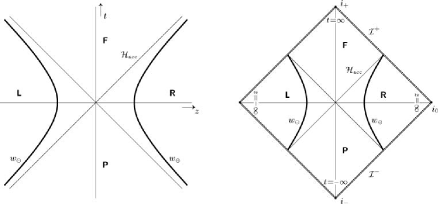
Figure 1: A pair of uniformly accelerated charges in Minkowski spacetime (with the conformal diagram on the right). The boost Killing vector is timelike in regions L and R; it is spacelike in F and P. The charges are causally disconnected by null hypersurfaces (“the roof”) ${-t^{2}+z^{2}=0}$. These hypersurfaces represent the acceleration horizon for uniformly accelerated observers with respect to which the charges are at rest.

The worldlines of the particles coincide with the orbits of the boost Killing vector in the $t{\text{-}}z$ plane,

$${\mathrm{\xi}}_{{\scriptscriptstyle{\mathrm{boost}}}}=z{\frac{\partial}{\partial t}}+t{\frac{\partial}{\partial z}}{\mbox{\;.}}$$ (5)

These orbits, given by ${-t^{2}+z^{2}=\text{constant}}$, ${x,\,y=\text{constant}}$, are timelike at ${-t^{2}+z^{2}>0}$, but they are spacelike at ${-t^{2}+z^{2}<0}$. The fields (scalar, electromagnetic, higher-spin) produced by charged particles in the hyperbolic motion will have boost-rotational symmetry. They are thus static in the region ${-t^{2}+z^{2}>0}$—“below the roof” as introduced in Bičák and Schmidt (1989), however, we can expect them to be radiative in the region ${-t^{2}+z^{2}<0}$—“above the roof”.

Consider a massless scalar field $\Phi$ with the scalar charge source $S$ satisfying, in a general 4-dimensional spacetime, the wave equation

$$\bigl{[}\square-{\textstyle\frac{1}{6}}R\bigr{]}\,\Phi=S{\mbox{\;,}}$$ (6)

in which ${\square\equiv{\mathrm{\mathit{g}}}^{\mu\nu}\nabla_{\mu}\nabla_{\nu}}$ is the curved-space d’Alambertian, and $R$ is the scalar curvature (of course, in Minkowski space $R=0$). We are interested in a field due to two monopole particles with the same constant scalar charge of magnitude $s$ moving along hyperbolae (3). The source at a spacetime point $x$ is thus given by

$$S=S_{\scriptscriptstyle{\oplus}}+S_{\scriptscriptstyle{\ominus}}{\mbox{\;,\quad}}S_{\varepsilon}=s\int\delta(x-w_{\varepsilon}(\lambda_{\scriptscriptstyle{\mathrm{M}}}))\,d\lambda_{\scriptscriptstyle{\mathrm{M}}}{\mbox{\;,}}$$ (7)

where $w_{\varepsilon}(\lambda_{\scriptscriptstyle{\mathrm{M}}})$ denotes the worldlines of the particles. The resulting fields may be written as

$$\Phi=\Phi_{\scriptscriptstyle{\oplus}}+\Phi_{\scriptscriptstyle{\ominus}}{\mbox{\;,}}$$ (8)

where $\Phi_{\varepsilon}$ is produced by $S_{\varepsilon}$. The retarded and advanced fields of these sources are constructed and analyzed in detail in Ref. Bičák and Schmidt (1989). It can be demonstrated that the retarded and advanced fields due to the particle $w_{\scriptscriptstyle{\oplus}}$ or $w_{\scriptscriptstyle{\ominus}}$ are all given by exactly identical expression

$$\Phi_{\scriptscriptstyle{\mathrm{BM}}}=\frac{s}{4\pi}\frac{1}{{\mathcal{R}}}{\mbox{\;,}}$$ (9)

which, however, is valid in different regions of spacetime. Namely,

$$\Phi_{{\scriptscriptstyle{\mathrm{ret}}}/{\scriptscriptstyle{\mathrm{adv}}}\,\varepsilon}=\frac{s}{4\pi}\frac{1}{{\mathcal{R}}}\;\theta(\varepsilon z\pm t){\mbox{\;,}}$$ (10)

$\theta$ being the step function and upper/lower sign is valid for retarded/advanced case. The quantity ${\mathcal{R}}$ in the denominator is given by

$${\mathcal{R}}=\frac{1}{2b_{\mathrm{o}}}\Bigl{(}\bigl{(}b_{\mathrm{o}}^{2}+t^{2}-r^{2}\bigr{)}^{2}+4b_{\mathrm{o}}^{2}r^{2}\sin^{2}\vartheta\Bigr{)}^{\frac{1}{2}}{\mbox{\;.}}$$ (11)

It has the meaning of a retarded or advanced distance—it is a spatial distance of the “observation” (field) point from the position of the source at retarded or advanced time. Here, as usual, $x=r\sin\vartheta\cos\varphi$, $y=r\sin\vartheta\sin\varphi$, $z=r\cos\vartheta$. The fields (9), as well as (10), are, at first glance, axially (rotationally) symmetric. They are also unchanged under the boost along the $z$ axis.

The field $\Phi_{\scriptscriptstyle{\mathrm{BM}}}$ can, in fact, be viewed as the field due to both accelerated particles, i.e., as the field corresponding to the source (7). Inspecting regions at which the retarded and advanced fields (10) are non-vanishing we discover that $\Phi_{\scriptscriptstyle{\mathrm{BM}}}$ admits the interpretation as arising from 1-parametric combination of retarded and advanced effects from both particles:

$$\Phi_{\scriptscriptstyle{\mathrm{BM}}}=\xi\Phi_{{\scriptscriptstyle{\mathrm{ret}}}{\scriptscriptstyle{\oplus}}}+(1-\xi)\Phi_{{\scriptscriptstyle{\mathrm{adv}}}{\scriptscriptstyle{\oplus}}}+(1-\xi)\Phi_{{\scriptscriptstyle{\mathrm{ret}}}{\scriptscriptstyle{\ominus}}}+\xi\Phi_{{\scriptscriptstyle{\mathrm{adv}}}{\scriptscriptstyle{\ominus}}}{\mbox{\;,}}$$ (12)

where $\xi\in{\mathbb{R}}$ is an arbitrary constant parameter. In particular, choosing ${\xi=\frac{1}{2}}$, the field $\Phi_{\scriptscriptstyle{\mathrm{BM}}}$ arises from ${\frac{1}{2}(\Phi_{\scriptscriptstyle{\mathrm{ret}}}+\Phi_{\scriptscriptstyle{\mathrm{adv}}})}$ from both particles. With ${\xi=1}$, the field can be interpreted as being caused by purely retarded effects from particle $w_{\scriptscriptstyle{\oplus}}$ in region ${z+t>0}$, and by purely advanced effects from particle $w_{\scriptscriptstyle{\ominus}}$ in region ${z+t<0}$.

The case of electrodynamics is very similar. The solution corresponding to the scalar field (9) was found by Born in 1909 Born (1909). It is customarily given in cylindrical coordinates (see, e.g., Rohrlich (1965); Fulton and Rohrlich (1960); Eriksen and Grøn (2000a)), however, in order to compare it with its generalization to de Sitter universe, it is more convenient to write it down in spherical coordinates:

$$\begin{split}{\mathrm{F}}_{\scriptscriptstyle{\mathrm{BM}}}=-\frac{e}{4\pi}&\frac{1}{2b_{\mathrm{o}}}\,\frac{1}{{\mathcal{R}}^{3}}\\ \times\Bigl{(}\!&-(b_{\mathrm{o}}^{2}+t^{2}-r^{2})\,\cos\vartheta\,{\mathrm{\mathrm{d}}}t\wedge{\mathrm{\mathrm{d}}}r\\ &+(b_{\mathrm{o}}^{2}+t^{2}+r^{2})\,r\sin\vartheta\,{\mathrm{\mathrm{d}}}t\wedge{\mathrm{\mathrm{d}}}\vartheta\\ &-2\,t\,r^{2}\sin\vartheta\,{\mathrm{\mathrm{d}}}r\wedge{\mathrm{\mathrm{d}}}\vartheta\Bigr{)}{\mbox{\;.}}\end{split}$$ (13)

The field can be obtained from the Liénard-Wiechert retarded and advanced potentials of two charged particles moving along hyperbolae (3), however, in contrast to the scalar case when charges are exactly the same, the electric charges have opposite signs. Similarly to the scalar case, the field is smooth everywhere, except for the places where the particles occur. ${\mathrm{F}}_{\scriptscriptstyle{\mathrm{BM}}}$ can be interpreted in the precisely same way as the scalar field (9), i.e., as the 1-parametric combination of retarded and advanced effects from both charges, analogously to Eq. (12). However, in the electromagnetic case an exact form of retarded and advanced fields from a single particle is a more subtle issue. Considering that the field in the region ${z+t>0}$ may be interpreted as the retarded effect emitted from the charge which moves along ${z>0}$, it is natural to try to exclude advanced effects of the other particle by requiring the field to vanish in the region ${z+t<0}$ (cf. Fig. 1). The field is then not smooth at the null hypersurface ${z=-t}$. In the scalar case such a field does represent the pure retarded field of the single particle, cf. Eq. (10). However, in the electromagnetic case the field ${{\mathrm{F}}_{\scriptscriptstyle{\mathrm{BM}}}\,\theta(z+t)}$ corresponds to sources consisting not only of the particle but also of a “charged wall” moving along hypersurface ${z+t=0}$ with velocity of light Leibovitz and Peres (1963); Bondi (1981). Nevertheless, it is possible to obtain a pure retarded field of the only single particle by modifying the field with a delta function valued term localized on ${z+t=0}$ Boulware (1980); Bondi and Gold (1955); Krtouš (1991).

In de Sitter space such a modification is not feasible because the advanced fields cannot be excluded. The underlying cause is the null character of the past conformal infinity in Minkowski spacetime, whereas in de Sitter spacetime both future and past conformal infinities are spacelike. As a consequence, the Gauss constraint restricts the data at the spacelike past infinity, and it can be shown that a purely retarded field of a point-like charge cannot satisfy this constraint Bičák and Krtouš (2001). The absence of purely retarded fields is also related to a different character of the past horizon of a particle. Since the worldline of a particle “enters” the universe through the past spacelike infinity, there exists the past particle horizon, called also the creation light cone. In de Sitter space a purely retarded electromagnetic field of a point-like charge cannot be constructed on the whole cone. In Minkowski spacetime the creation light cone of a particle moving asymptotically in the past freely, coincides with the whole past null infinity, and thus it does not belong to the physical spacetime. Eternally accelerated particles can “enter” the Minkowski spacetime at a point of the past null infinity—as, for example, uniformly accelerated particles do. Like in de Sitter case, in conformal spacetime the past horizon of such particles forms the null cone but, in contrast to de Sitter space, it has one generator in common with the null infinity. In physical spacetime this horizon thus corresponds to a null hyperplane—for the particle $w_{\scriptscriptstyle{\oplus}}$ it is just the hyperplane ${z+t=0}$ (cf. Fig. 1)—and so its spatial sections are not compact. Thanks to this non-compactness the “bad” behavior of the retarded field on the horizon can be “pushed out of sight” to the infinity. We analyzed this issue in detail in Ref. Bičák and Krtouš (2001).

III Many faces of de Sitter

The fields due to various types of uniformly accelerated sources in de Sitter spacetime found in Bičák and Krtouš (2001), as well as those described briefly in Ref. Bičák and Krtouš (2002), were constructed by employing the conformal relation between Minkowski and de Sitter spacetimes. When analyzing the worldlines of the sources in de Sitter spacetime and their relation to the corresponding worldlines in Minkowski spacetime we need to introduce appropriate coordinate systems. Suitable coordinates will later be used to exhibit various properties of the fields. An extensive literature exists on various types of coordinates in de Sitter space (e.g. Schmidt (1993); Eriksen and Grøn (1995)), but we want to survey some of them in this section. In particular, we relate them to the corresponding coordinates on conformally related Minkowski spaces since this does not appear to be given elsewhere. In the next section, after identifying the worldlines of uniformly accelerated particles in de Sitter space, we shall construct new coordinate systems tied to such particles, such as Rindler-type “accelerated” coordinates, or Robinson-Trautman-type coordinates in which the null cones emanating from the particles have especially simple forms. These coordinate systems will turn out to be very useful in analyzing the fields. Here, in the main text, however, only a brief description of relevant coordinates will be given. More details, including both formulas and illustrations, are relegated to the Appendix.

As it is well-known from textbooks on general relativity (for a recent pedagogical exposition, see Rindler (2001)), de Sitter spacetime, which is the solution of Einstein vacuum equations with a cosmological term ${\Lambda>0}$, is best visualized as the 4-dimensional hyperboloid imbedded in flat 5-dimensional Minkowski space. It is the homogeneous space of constant curvature equal to $4\Lambda$. Hereafter, we use the quantity

$$\ell_{\scriptscriptstyle\Lambda}=\sqrt{\frac{3}{\Lambda}}$$ (14)

(with the dimension of length) to parametrize the radius of the curvature.

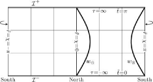
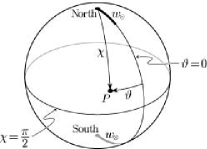
Figure 2: The spherical cosmological coordinates and a pair of uniformly accelerated particles ${w_{\scriptscriptstyle{\odot}}}$ and ${w_{\scriptscriptstyle{\otimes}}}$ in de Sitter universe: the conformal diagram (above) and projection on the spacelike cut ${\tau=\text{constant}}$ in the standard cosmological spherical coordinates (angle $\varphi$ suppressed). The whole de Sitter spacetime could be represented by just the “right half” of the conformal diagram. For convenience, we admit negative values of radial coordinates and identify ${{\tilde{r}}=\chi=-\pi}$ and ${{\tilde{r}}=\chi=\pi}$ (see the text below Eq. (25) and the Appendix).

The entire de Sitter spacetime can be covered by a single coordinate system—which we call standard coordinates—$\tau\in{\mathbb{R}}$, $\chi\in(0,\pi)$, $\vartheta\in(0,\pi)$, $\varphi\in(-\pi,\pi)$ in which the metric reads

$${\mathrm{\mathit{g}}}_{\scriptscriptstyle{\mathrm{dS}}}=-{\mathrm{\mathrm{d}}}\tau{}^{2}+\ell_{\scriptscriptstyle\Lambda}^{2}\cosh^{2}\!\frac{\tau}{\ell_{\scriptscriptstyle\Lambda}}\;\Bigl{(}{\mathrm{\mathrm{d}}}\chi{}^{2}+\sin^{2}\!\chi\;{{\mathrm{\mathrm{d}\omega}}^{2}}\Bigr{)}{\mbox{\;,}}$$ (15)

$${{\mathrm{\mathrm{d}\omega}}^{2}}={\mathrm{\mathrm{d}}}\vartheta{}^{2}+\sin^{2}\vartheta\,{\mathrm{\mathrm{d}}}\varphi{}^{2}{\mbox{\;.}}$$ (16)

Clearly, we can imagine the spacetime as the time evolution of a 3-sphere which shrinks from infinite extension at $\tau\to-\infty$ to a radius $\ell_{\scriptscriptstyle\Lambda}$, and then expands again in a time-symmetric way. Hence, we also call ${\tau,\,\chi}$ the spherical cosmological coordinates. The coordinate lines are shown in the conformal diagram, Fig. 2.

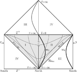
Figure 3: The flat cosmological coordinates and particles ${w_{\scriptscriptstyle{\odot}}}$, ${w_{\scriptscriptstyle{\otimes}}}$ in de Sitter space and in conformally related Minkowski space. The flat cosmological coordinates cover shaded region. Its boundary, ${{\check{r}}=\pm\infty}$, represents the horizon for observers at rest in these coordinates.

In cosmology the most popular “flat” de Sitter universe is obtained by considering only a half of de Sitter hyperboloid foliated by flat 3-dimensional spacelike hypersurfaces labeled by timelike coordinate ${{\check{\tau}}\in{\mathbb{R}}}$, cf. Fig. 3. Together with appropriate radial coordinate ${{\check{r}}\in{\mathbb{R}}^{+}}$, the new coordinates, which we call flat cosmological coordinates, are given in terms of ${\tau,\,\chi}$ by

$${\check{\tau}} =\ell_{\scriptscriptstyle\Lambda}\log\Bigl{(}\sinh\frac{\tau}{\ell_{\scriptscriptstyle\Lambda}}+\cosh\frac{\tau}{\ell_{\scriptscriptstyle\Lambda}}\,\cos\chi\Bigr{)}{\mbox{\;,}}$$ (17)

$${\check{r}} =\ell_{\scriptscriptstyle\Lambda}\frac{\sin\chi}{\cos\chi+\tanh(\tau/\ell_{\scriptscriptstyle\Lambda})}{\mbox{\;,}}$$

implying the well-known “inflationary” metric

$${\mathrm{\mathit{g}}}_{\scriptscriptstyle{\mathrm{dS}}}=-{\mathrm{\mathrm{d}}}{\check{\tau}}{}^{2}+\exp{\frac{2{\check{\tau}}}{\ell_{\scriptscriptstyle\Lambda}}}\;\Bigl{(}{\mathrm{\mathrm{d}}}{\check{r}}{}^{2}+{\check{r}}^{2}\,{{\mathrm{\mathrm{d}\omega}}^{2}}\Bigr{)}{\mbox{\;.}}$$ (18)

These coordinates cover only “one-half” of de Sitter space as indicated by shading in Fig. 3.

de Sitter introduced his model in what we call hyperbolic cosmological coordinates ${\eta\in{\mathbb{R}}}$, ${\rho\in{\mathbb{R}}^{+}}$ (see Fig. 4) related to ${\tau,\,\chi}$ by

$$\cosh\frac{\eta}{\ell_{\scriptscriptstyle\Lambda}} =\cosh\frac{\tau}{\ell_{\scriptscriptstyle\Lambda}}\,\cos\chi{\mbox{\;,}}$$ (19)

$$\tanh\frac{\rho}{\ell_{\scriptscriptstyle\Lambda}} =\coth\frac{\tau}{\ell_{\scriptscriptstyle\Lambda}}\,\sin\chi{\mbox{\;.}}$$

The metric

$${\mathrm{\mathit{g}}}_{\scriptscriptstyle{\mathrm{dS}}}=-{\mathrm{\mathrm{d}}}\eta{}^{2}+\sinh^{2}\!\frac{\eta}{\ell_{\scriptscriptstyle\Lambda}}\,\Bigl{(}{\mathrm{\mathrm{d}}}\rho{}^{2}+\ell_{\scriptscriptstyle\Lambda}^{2}\,{\sinh^{2}\!\frac{\rho}{\ell_{\scriptscriptstyle\Lambda}}}\;{{\mathrm{\mathrm{d}\omega}}^{2}}\Bigr{)}$$ (20)

shows that the time slices ${\eta=\text{constant}}$ have the geometry of constant negative curvature, i.e., as the standard time slices in an open FRW universe.

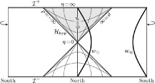
Figure 4: The hyperbolic cosmological coordinates. They cover only the shaded region and, therefore, only a part of the worldline ${w_{\scriptscriptstyle{\odot}}}$. The horizon ${{\mathcal{H}}_{\scriptscriptstyle{\mathrm{hyp}}}}$ arises for the observers who are at rest in the hyperbolic cosmological coordinates.

The last commonly used coordinates in de Sitter spacetime are static coordinates ${T\in{\mathbb{R}}}$, ${R\in(0,\ell_{\scriptscriptstyle\Lambda})}$:

$$T =\frac{\ell_{\scriptscriptstyle\Lambda}}{2}\,\log\left\lvert\frac{\cos\chi+\tanh(\tau/\ell_{\scriptscriptstyle\Lambda})}{\cos\chi-\tanh(\tau/\ell_{\scriptscriptstyle\Lambda})}\right\rvert{\mbox{\;,}}$$ (21)

$$R =\ell_{\scriptscriptstyle\Lambda}\cosh\frac{\tau}{\ell_{\scriptscriptstyle\Lambda}}\;\sin\chi{\mbox{\;,}}$$

covering also only a part of the universe. The metric in these coordinates reads

$${\mathrm{\mathit{g}}}_{\scriptscriptstyle{\mathrm{dS}}}=-\Bigl{(}1-\frac{R^{2}}{\ell_{\scriptscriptstyle\Lambda}^{2}}\Bigr{)}\,{\mathrm{\mathrm{d}}}T{}^{2}+\Bigl{(}1-\frac{R^{2}}{\ell_{\scriptscriptstyle\Lambda}^{2}}\Bigr{)}^{\!\!-1}\!{\mathrm{\mathrm{d}}}R{}^{2}+R^{2}\,{{\mathrm{\mathrm{d}\omega}}^{2}}{\mbox{\;,}}$$ (22)

revealing that ${{\partial}/{\partial T}}$ is a timelike Killing vector in the region ${0<R<\ell_{\scriptscriptstyle\Lambda}}$.

Among the coordinates introduced until now only the standard coordinates ${\tau,\,\chi,\,\vartheta,\,\varphi}$ cover the whole de Sitter spacetime globally. One can easily extend flat cosmological coordinates to cover (though not smoothly) the whole de Sitter hyperboloid, which will be useful in discussion of the conformally related Minkowski spacetime, cf. Eq. (26). We shall also use extensions of the static coordinates into the whole spacetime, using definitions (21), but allowing $R\in{\mathbb{R}}^{+}$. In regions where $R>\ell_{\scriptscriptstyle\Lambda}$ coordinates $T$ and $R$ interchange their character, ${{\partial}/{\partial T}}$ becomes a spacelike Killing vector (analogously to ${{\partial}/{\partial t}}$ inside a Schwarzschild black hole). However, the static coordinates ${T,\,R}$ are not globally smooth and uniquely valued. Namely, ${T\to\infty}$ at the cosmological horizons $R=\ell_{\scriptscriptstyle\Lambda}$. The static coordinates, extended to the whole de Sitter space, are illustrated in Fig. 5. Here we also indicate the regions in which ${{{\partial}/{\partial T}}}$ is spacelike by bold F (“future”) and P (“past”), whereas the regions in which it is timelike are denoted by N (containing the “north pole” ${\chi=0}$) and S (containing the “south pole” ${\chi=\pi}$). Hereafter, this notation will be used repeatedly.

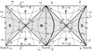
Figure 5: The static coordinates and the wordlines of particles ${w_{\scriptscriptstyle{\odot}}}$ and ${w_{\scriptscriptstyle{\otimes}}}$. These coordinates can be defined in the whole spacetime, however several coordinate patches, in diagram indicated by shaded and nonshaded regions, have to be used (cf. Appendix A.5 and A.6). These regions are separated by the cosmological horizons at ${R=\ell_{\scriptscriptstyle\Lambda}}$, where ${T=\pm\infty}$. The vector ${{\partial}/{\partial T}}$ is a Killing vector of de Sitter spacetime. It is timelike in the domains N and S (shaded regions) and spacelike in the domains F and P. The histories of both particles ${w_{\scriptscriptstyle{\odot}}}$ and ${w_{\scriptscriptstyle{\otimes}}}$ belong to the domains N and S.

The conformal structure of Minkowski and de Sitter spacetimes, their conformal relation, and their conformal relation to various regions of the Einstein static universe have been discussed extensively in literature (see, e.g., Penrose (1968); Penrose and Rindler (1984, 1986); Hawking and Ellis (1973); Wald (1984)). The complete compactified picture of these spacetimes, in particular the 3-dimensional diagram of the compactified Minkowski and de Sitter spaces $M^{\#}$ as parts of the Einstein universe represented by a solid cylinder can be found in Bičák and Krtouš (2001). We refer the reader especially to Section III of Bičák and Krtouš (2001) where we explain and illustrate the compactification in detail. In the present paper we shall confine ourselves to the 2-dimensional Penrose diagrams.

The basic standard rescaled coordinates covering globally de Sitter spacetime including the conformal infinity are simply related to the standard coordinates as follows:

$$\tan\frac{{\tilde{t}}}{2}=\exp\frac{\tau}{\ell_{\scriptscriptstyle\Lambda}}{\mbox{\;,\quad}}{\tilde{r}}=\chi{\mbox{\;,}}$$ (23)

${{\tilde{t}}\in(0,\pi)}$, ${{\tilde{r}}\in(0,\pi)}$. The metric (15) becomes

$${\mathrm{\mathit{g}}}_{\scriptscriptstyle{\mathrm{dS}}}=\ell_{\scriptscriptstyle\Lambda}^{2}\,\sin^{\!-2}\!{\tilde{t}}\;\bigl{(}-{\mathrm{\mathrm{d}}}{\tilde{t}}{}^{2}+{\mathrm{\mathrm{d}}}{\tilde{r}}{}^{2}+\sin^{2}{\tilde{r}}\,{{\mathrm{\mathrm{d}\omega}}^{2}}\bigr{)}{\mbox{\;,}}$$ (24)

demonstrating explicitly the conformal relations of de Sitter spacetime to the Einstein universe:

$${\mathrm{\mathit{g}}}_{\scriptscriptstyle{\mathrm{E}}}=\Omega_{\scriptscriptstyle{\mathrm{dS}}}^{2}\,{\mathrm{\mathit{g}}}_{\scriptscriptstyle{\mathrm{dS}}}{\mbox{\;,\quad}}\Omega_{\scriptscriptstyle{\mathrm{dS}}}=\sin{\tilde{t}}{\mbox{\;.}}$$ (25)

Therefore, we also call coordinates ${{\tilde{t}},\,{\tilde{r}}}$ the conformally Einstein coordinates. The conformal diagram of de Sitter spacetime is illustrated in Fig. 2. The past and future infinities, ${{\tilde{t}}=0}$ and ${{\tilde{t}}=\pi}$ are spacelike, the worldlines of the north and south poles (given by the choice of the origin of the coordinates) are described by ${{\tilde{r}}=\chi=0}$ and ${{\tilde{r}}=\chi=\pi}$.

The whole de Sitter spacetime could be represented by just the “right half” of Fig. 2. Indeed, it is customary to draw this half only and to consider any point in the figure as a 2-sphere, except for the poles ${{\tilde{r}}=0,\pi}$. As we shall see, the formulas relating coordinates on the conformally related de Sitter and Minkowski spacetimes have simpler forms if we admit negative values of the radial coordinate ${{\tilde{r}}\in(-\pi,0)}$ covering the left half of the diagram. We shall thus consider the 2-dimensional diagrams as in Fig. 2 to represent the cuts of de Sitter spacetime along the axis going through the origins (through north and south poles—analogously to the cuts along the $z$ axis in $E^{3}$). The axis, i.e., the main circle of the spatial spherical section of de Sitter spacetime, is typically chosen as ${\vartheta=0,\pi}$. Thus, in the diagram the point with ${{\tilde{r}}=-{\tilde{r}}_{\mathrm{o}}<0}$, ${\vartheta=\vartheta_{\mathrm{o}}}$, ${\varphi=\varphi_{\mathrm{o}}}$ is identical to that with ${{\tilde{r}}={\tilde{r}}_{\mathrm{o}}}$, ${\vartheta=\pi-\vartheta_{\mathrm{o}}}$, and ${\varphi=\varphi_{\mathrm{o}}+\pi}$. We use the same convention also for other radial coordinates appearing later, as explicitly stated in the Appendix (cf. also Appendix in Bičák and Krtouš (2001)). We admit negative radial coordinates only when describing various relations between the coordinate systems. In the expressions for the fields in the following sections only positive radial coordinates are considered.

As mentioned above, in Bičák and Krtouš (2001) we constructed fields on de Sitter spacetime by conformally transforming the fields from Minkowski spacetime. Now “different Minkowski spaces” can be used in the conformal relation to de Sitter space, depending on which region of a Minkowski space is mapped onto which region of de Sitter space. Consider, for example, Minkowski space with metric ${\mathrm{\mathit{g}}}_{\scriptscriptstyle{\mathrm{M}}}$ given in spherical coordinates ${{\check{t}},\,{\check{r}},\,\vartheta,\,\varphi}$. Identify it with de Sitter space by relations

$${\check{t}}=\frac{\ell_{\scriptscriptstyle\Lambda}\sin{\tilde{t}}}{\cos{\tilde{t}}-\cos{\tilde{r}}}{\mbox{\;,\quad}}{\check{r}}=\frac{\ell_{\scriptscriptstyle\Lambda}\sin{\tilde{r}}}{\cos{\tilde{r}}-\cos{\tilde{t}}}{\mbox{\;,}}$$ (26)

the inverse relation (145) is given in the Appendix. In the coordinates ${{\check{t}},\,{\check{r}},\,\vartheta,\,\varphi}$ the de Sitter metric (24) becomes

$${\mathrm{\mathit{g}}}_{\scriptscriptstyle{\mathrm{dS}}}=\frac{\ell_{\scriptscriptstyle\Lambda}^{2}}{{\check{t}}^{2}}\,\Bigl{(}-{\mathrm{\mathrm{d}}}{\check{t}}{}^{2}+{\mathrm{\mathrm{d}}}{\check{r}}{}^{2}+{\check{r}}^{2}\,{{\mathrm{\mathrm{d}\omega}}^{2}}\Bigr{)}{\mbox{\;,}}$$ (27)

so that

$${\mathrm{\mathit{g}}}_{\scriptscriptstyle{\mathrm{dS}}}=\Omega_{\scriptscriptstyle{\mathrm{\check{M}}}}^{2}{\mathrm{\mathit{g}}}_{\scriptscriptstyle{\mathrm{\check{M}}}}{\mbox{\;,\quad}}\Omega_{\scriptscriptstyle{\mathrm{\check{M}}}}=\frac{\ell_{\scriptscriptstyle\Lambda}}{{\check{t}}}{\mbox{\;.}}$$ (28)

The coordinates ${{\check{t}},\,{\check{r}},\,\vartheta,\,\varphi}$ can, of course, be used in both de Sitter and Minkowski spaces. Fig. 3 illustrates the coordinate lines. It also shows how four regions I, II, III, and IV of Minkowski space are mapped onto four regions of de Sitter space by relations (26). We call ${{\check{t}},\,{\check{r}}}$ rescaled flat cosmological coordinates since their radial coordinate ${\check{r}}$ coincides with that of the flat cosmological coordinates (17) and the time coordinate is simply related to ${\check{\tau}}$ as

$${\check{t}}=-\ell_{\scriptscriptstyle\Lambda}\,\exp(-{\check{\tau}}/\ell_{\scriptscriptstyle\Lambda}){\mbox{\;.}}$$ (29)

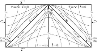
Figure 16: The flat cosmological family, type “$\wedge$”.

The caron or the check (still better “háček”) “$\vee$” formed by cosmological horizon at ${{\check{t}}=\pm\infty}$ in de Sitter space (cf. Fig. 3) inspired our notation of these coordinates. It is possible to introduce analogously the coordinates ${{\hat{t}},\,{\hat{r}}}$ given in the Appendix, Eqs. (173), (174), that cover nicely the past conformal infinity but are not smooth at the cosmological horizon ${{\hat{t}}=\pm\infty}$; in this case they form the hat “$\wedge$” in the conformal diagram (see Fig. 16 in the Appendix).

From relations (26) it is explicitly seen why, when writing down mappings between de Sitter and Minkowski spaces and drawing the corresponding 2-dimensional conformal diagrams, it is advantageous to admit negative radial coordinates. If we would restrict all radial coordinates to be non-negative, we would have to consider the second relation in Eq. (26) with different signs for regions III and II in de Sitter space: in III ${{\check{r}}={\ell_{\scriptscriptstyle\Lambda}\sin{\tilde{r}}}/{(\cos{\tilde{r}}-\cos{\tilde{t}})}}$, but in III we would have ${{\check{r}}=-{\ell_{\scriptscriptstyle\Lambda}\sin{\tilde{r}}}/{(\cos{\tilde{r}}-\cos{\tilde{t}})}}$.

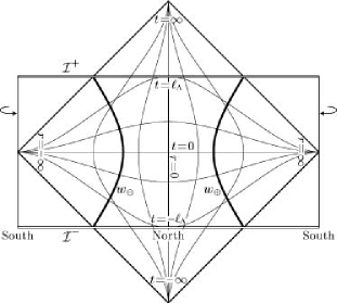
Figure 6: The conformally Minkowski coordinates. They cover the whole conformally related Minkowski space but only a part of corresponding de Sitter space. This Minkowski space is related to that in Fig. 3 by a shift “downwards” by ${\pi/2}$ in the direction of the conformally Einstein coordinate ${\tilde{t}}$.

Another mapping of Minkowski on de Sitter space will be used to advantage in the explicit manifestation that the generalized Born solution in de Sitter space goes over to the classical solution (13). Instead of the mapping (26), consider the relations

$$t=-\frac{\ell_{\scriptscriptstyle\Lambda}\cos{\tilde{t}}}{\cos{\tilde{r}}+\sin{\tilde{t}}}{\mbox{\;,\quad}}r=\frac{\ell_{\scriptscriptstyle\Lambda}\sin{\tilde{r}}}{\cos{\tilde{r}}+\sin{\tilde{t}}}$$ (30)

(see Eq. (151) for the inverse mapping), which turn the metric (24) into

$${\mathrm{\mathit{g}}}_{\scriptscriptstyle{\mathrm{dS}}}=\Bigl{(}\frac{2\,\ell_{\scriptscriptstyle\Lambda}^{2}}{\ell_{\scriptscriptstyle\Lambda}^{2}-t^{2}+r^{2}}\Bigr{)}^{2}\,\Bigl{(}-{\mathrm{\mathrm{d}}}t{}^{2}+{\mathrm{\mathrm{d}}}r{}^{2}+r^{2}\,{{\mathrm{\mathrm{d}\omega}}^{2}}\Bigr{)}{\mbox{\;.}}$$ (31)

We again obtain the de Sitter metric in the form explicitly conformal to the Minkowski metric with, however, a different conformal factor from that in Eq. (28):

$${\mathrm{\mathit{g}}}_{\scriptscriptstyle{\mathrm{dS}}}=\Omega_{\scriptscriptstyle{\mathrm{M}}}^{2}\,{\mathrm{\mathit{g}}}_{\scriptscriptstyle{\mathrm{M}}}{\mbox{\;,\quad}}\Omega_{\scriptscriptstyle{\mathrm{M}}}=\frac{2\,\ell_{\scriptscriptstyle\Lambda}^{2}}{\ell_{\scriptscriptstyle\Lambda}^{2}-t^{2}+r^{2}}{\mbox{\;.}}$$ (32)

(For the use of the de Sitter metric in “atypical” form (31) in the work on the domain wall spacetimes, see Cvetič et al. (1993).) The relation of Minkowski space to de Sitter space based on the mapping (30) is illustrated in Fig. 6. Clearly, the Minkowski space in this figure is shifted “downwards” by ${\pi/2}$ in ${{\tilde{t}}}$ coordinate, as compared with Minkowski space in Fig. 3 (Eq. (26)). Indeed, replacing ${{\tilde{t}}}$ by ${{\tilde{t}}+\frac{\pi}{2}}$ in Eq. (26), we get ${{\check{t}}=t}$, ${{\check{r}}=r}$ with ${t,\,r}$ given by Eq. (30). Since coordinates ${t,\,r,\,\vartheta,\varphi}$ are not connected directly with any cosmological model and correspond to Minkowski space “centered” on de Sitter space (Fig. 6), we just call them conformally Minkowski coordinates.

In Ref. Bičák and Krtouš (2001) still another Minkowski space is related to de Sitter space—one which is shifted “downward” in ${{\tilde{t}}}$ coordinate by another ${\pi/2}$. As mentioned below Eq. (29), the cosmological horizon forms hat “${\wedge}$” in this case and the corresponding coordinates are accordingly denoted as ${{\hat{t}},\,{\hat{r}}}$. They are given explicitly in Appendix A.3 and Fig. 16.

The three sets of coordinates ${{\check{t}},\,{\check{r}}}$, $\;{t,\,r}$, and ${{\hat{t}},\,{\hat{r}}}$ (with the same ${\vartheta,\,\varphi}$) relating naturally “three” Minkowski spaces to de Sitter space are suitable for different purposes. The third set describes conveniently the past infinity of de Sitter space—that is why it was used extensively in Bičák and Krtouš (2001) where we were interested in how the sources enter (are “born in”) de Sitter universe. The second set will be needed in Section VII for exhibiting the flat-space limit of the generalized Born solution. The first set describes nicely the future infinity and will be employed when analyzing radiative properties of the fields.

With all the coordinates discussed above, corresponding double null coordinates can be associated; some of them will also be used in the following. Their more detailed description and illustration is presented in section A.10 of the Appendix.

Before concluding this section let us notice that the observers which are at rest in cosmological coordinate systems ${\tau,\,\chi}$, $\;{{\check{\tau}},\,{\check{r}}}$, and ${\eta,\,\rho}$ move along the geodesics with proper time $\tau$, ${\check{\tau}}$, and ${\eta}$ respectively. These geodesics are also the orbits of the conformal Killing vectors. Indeed, the symmetries of Minkowski spacetime and of the Einstein universe become conformal symmetries in conformally related de Sitter spacetime. In particular, we shall employ the fact that since ${{{\partial}/{\partial{\check{t}}}}}$ and ${{{\partial}/{\partial t}}}$ are timelike Killing vectors in Minkowski spacetime and ${{{\partial}/{\partial{\tilde{t}}}}}$ is a timelike Killing vector in the Einstein universe, the vectors

$${\frac{\partial}{\partial{\tilde{t}}}}{\mbox{\;,\quad}}{\frac{\partial}{\partial{\check{t}}}}{\mbox{\;,\quad}}\text{and}\quad{\frac{\partial}{\partial t}}$$ (33)

are timelike conformal Killing vectors in de Sitter spacetime. As mentioned below Eq. (22), ${{{\partial}/{\partial T}}}$ is a Killing vector which is timelike for ${\left\lvert R\right\rvert<\ell_{\scriptscriptstyle\Lambda}}$.

IV Uniformly accelerated particles in de Sitter

IV.1 Particles born at the poles

In Section II we defined uniformly accelerated motion in Minkowski spacetime. However, the formulas given there, being in covariant forms, remain valid in de Sitter spacetime. As explained in Bičák and Krtouš (2001) in detail, a simple way of obtaining a worldline of a uniformly accelerated particle in de Sitter spacetime is to consider a suitable particle moving with a uniform velocity in Minkowski spacetime and use the conformal relation between the spaces.

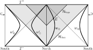
Figure 7: The worldlines of uniformly accelerated charges. The particles ${w_{\scriptscriptstyle{\odot}}}$ and ${w_{\scriptscriptstyle{\odot}}^{\prime}}$ start and end at the “north pole,” ${w_{\scriptscriptstyle{\otimes}}}$, ${w_{\scriptscriptstyle{\otimes}}^{\prime}}$ start and end at the south pole. Particles ${w_{\scriptscriptstyle{\odot}}^{\prime}}$, ${w_{\scriptscriptstyle{\otimes}}^{\prime}}$ have a higher magnitude of acceleration ${a_{\scriptscriptstyle{\mathrm{dS}}}}$ than particles ${w_{\scriptscriptstyle{\odot}}}$, ${w_{\scriptscriptstyle{\otimes}}}$. They are characterized by a negative parameter ${\alpha_{\mathrm{o}}}$, whereas particles ${w_{\scriptscriptstyle{\odot}}}$, ${w_{\scriptscriptstyle{\otimes}}}$ have a positive $\alpha_{\mathrm{o}}$.

Consider a particle moving with a constant velocity of magnitude

$$v_{\scriptscriptstyle{\mathrm{\check{M}}}}=\tanh\alpha_{\mathrm{o}}=\text{constant}{\mbox{\;,}}$$ (34)

such that for $\alpha_{\mathrm{o}}>0$ it moves in a negative direction along the ${{\check{z}}}$ axis of the inertial frame in Minkowski space ${\check{M}}$ with coordinates ${{\check{t}},\,{\check{r}},\,\vartheta,\,\varphi}$ and passes through ${{\check{r}}=0}$ at ${{\check{t}}=0}$:

$${\check{t}} =\lambda_{\scriptscriptstyle{\mathrm{\check{M}}}}\,\cosh\alpha_{\mathrm{o}}{\mbox{\;,}}$$ (35)

$${\check{r}} =-\lambda_{\scriptscriptstyle{\mathrm{\check{M}}}}\sinh\alpha_{\mathrm{o}}{\mbox{\;,\quad}}\vartheta=0{\mbox{\;.}}$$

Substituting into transformation (145), we find

$${\tilde{t}} =\arctan\Bigl{(}-2\ell_{\scriptscriptstyle\Lambda}\frac{\lambda_{\scriptscriptstyle{\mathrm{\check{M}}}}\cosh\alpha_{\mathrm{o}}}{\lambda_{\scriptscriptstyle{\mathrm{\check{M}}}}^{2}-\ell_{\scriptscriptstyle\Lambda}^{2}}\Bigr{)}{\mbox{\;,}}$$ (36)

$${\tilde{r}} =\arctan\Bigl{(}-2\ell_{\scriptscriptstyle\Lambda}\frac{\lambda_{\scriptscriptstyle{\mathrm{\check{M}}}}\sinh\alpha_{\mathrm{o}}}{\lambda_{\scriptscriptstyle{\mathrm{\check{M}}}}^{2}+\ell_{\scriptscriptstyle\Lambda}^{2}}\Bigr{)}{\mbox{\;,}}$$

or expressing Minkowski proper time ${\lambda_{\scriptscriptstyle{\mathrm{\check{M}}}}}$ in terms of the proper time of de Sitter spacetime,

$$\lambda_{\scriptscriptstyle{\mathrm{\check{M}}}}=\mp\ell_{\scriptscriptstyle\Lambda}\exp\bigl{(}\mp(\cosh\alpha_{\mathrm{o}})\,{\lambda_{\scriptscriptstyle{\mathrm{dS}}}}/\ell_{\scriptscriptstyle\Lambda}\bigr{)}{\mbox{\;,}}$$ (37)

we obtain

$${\tilde{t}} =\operatorname{arccot}\Bigl{(}-\frac{\sinh\bigl{(}(\cosh\alpha_{\mathrm{o}})\,{\lambda_{\scriptscriptstyle{\mathrm{dS}}}}/\ell_{\scriptscriptstyle\Lambda}\bigr{)}}{\cosh\alpha_{\mathrm{o}}}\Bigr{)}{\mbox{\;,}}$$ (38)

$${\tilde{r}} =\operatorname{arccot}\Bigl{(}\pm\frac{\cosh\bigl{(}(\cosh\alpha_{\mathrm{o}})\,{\lambda_{\scriptscriptstyle{\mathrm{dS}}}}/\ell_{\scriptscriptstyle\Lambda}\bigr{)}}{\sinh\alpha_{\mathrm{o}}}\Bigr{)}{\mbox{\;,\quad}}\vartheta=0{\mbox{\;.}}$$

Here ${\lambda_{\scriptscriptstyle{\mathrm{dS}}}\in{\mathbb{R}}}$, $\operatorname{arccot}{}$ takes values such that ${{\tilde{t}}\in(0,\pi)}$ and ${{\tilde{r}}\in(0,\pi)}$ for ${\alpha_{\mathrm{o}}>0}$, or ${{\tilde{r}}\in(-\pi,0)}$ for ${\alpha_{\mathrm{o}}<0}$. Upper sign is valid for the particle starting and ending with ${{\tilde{r}}=0}$ (particle ${w_{\scriptscriptstyle{\odot}}}$ in Fig. 7), lower sign for the particle starting and ending at ${{\tilde{r}}=\pi}$ (particle $w_{\scriptscriptstyle{\otimes}}$ in Fig. 7).

One can make sure by direct calculations of the four-acceleration (for its simplest form in the static coordinates, see below) that these worldlines describe the uniformly accelerated motion as defined in Section II, the magnitude of the acceleration being

$$a_{\scriptscriptstyle{\mathrm{dS}}}=\sqrt{{\mathrm{a}}^{\mu}{\mathrm{a}}_{\mu}}=\left\lvert\ell_{\scriptscriptstyle\Lambda}^{-1}\,\sinh\alpha_{\mathrm{o}}\right\rvert{\mbox{\;.}}$$ (39)

Since de Sitter universe represents the asymptotic state of all three types of indefinitely expanding FRW models with $\Lambda>0$, it is of interest to find out the form of these worldlines in the three types of cosmological frames—spherical, flat, and hyperbolic—introduced in Section II.

In terms of cosmological spherical coordinates the worldlines are given by

$$\tau =\ell_{\scriptscriptstyle\Lambda}\,\operatorname{arcsinh}\Biggl{(}\frac{\sinh\bigl{(}(\cosh\alpha_{\mathrm{o}})\,{\lambda_{\scriptscriptstyle{\mathrm{dS}}}}/\ell_{\scriptscriptstyle\Lambda}\bigr{)}}{\cosh\alpha_{\mathrm{o}}}\Biggr{)}{\mbox{\;,}}$$ (40)

$$\chi =\operatorname{arccot}\Biggl{(}\pm\frac{\cosh\bigl{(}(\cosh\alpha_{\mathrm{o}})\,{\lambda_{\scriptscriptstyle{\mathrm{dS}}}}/\ell_{\scriptscriptstyle\Lambda}\bigr{)}}{\sinh\alpha_{\mathrm{o}}}\Biggr{)}{\mbox{\;,\quad}}\vartheta=0{\mbox{\;.}}$$

In flat cosmological coordinates, which cover only half of de Sitter space, we obtain just particle $w_{\scriptscriptstyle{\odot}}$ described by the worldline

$${\check{\tau}} =\lambda_{\scriptscriptstyle{\mathrm{dS}}}\,\cosh\alpha_{\mathrm{o}}-\ell_{\scriptscriptstyle\Lambda}\log\cosh\alpha_{\mathrm{o}}{\mbox{\;,}}$$ (41)

$${\check{r}} =\ell_{\scriptscriptstyle\Lambda}\sinh\alpha_{\mathrm{o}}\;\,\exp\bigl{(}-(\cosh\alpha_{\mathrm{o}})\,{\lambda_{\scriptscriptstyle{\mathrm{dS}}}}/\ell_{\scriptscriptstyle\Lambda}\bigr{)}{\mbox{\;.}}$$

Finally, in hyperbolic cosmological coordinates, which are also not global, we obtain again one particle’s worldline only given in terms of its proper time as

$$\eta =\ell_{\scriptscriptstyle\Lambda}\operatorname{arccosh}\frac{\cosh\bigl{(}(\cosh\alpha_{\mathrm{o}})\,{\lambda_{\scriptscriptstyle{\mathrm{dS}}}}/\ell_{\scriptscriptstyle\Lambda}\bigr{)}}{\cosh\alpha_{\mathrm{o}}}{\mbox{\;,}}$$ (42)

$$\rho =\ell_{\scriptscriptstyle\Lambda}\operatorname{arccoth}\frac{\sinh\bigl{(}(\cosh\alpha_{\mathrm{o}})\,{\lambda_{\scriptscriptstyle{\mathrm{dS}}}}/\ell_{\scriptscriptstyle\Lambda}\bigr{)}}{\sinh\alpha_{\mathrm{o}}}{\mbox{\;.}}$$

These formulas have no meaning for ${\left\lvert{\lambda_{\scriptscriptstyle{\mathrm{dS}}}}/\ell_{\scriptscriptstyle\Lambda}\;\cosh\alpha_{\mathrm{o}}\right\rvert<\left\lvert\alpha_{\mathrm{o}}\right\rvert}$ where the inverse hyperbolic functions are not defined. This corresponds to the fact that for such ${\lambda_{\scriptscriptstyle{\mathrm{dS}}}}$ the particle occurs in the region where the hyperbolic cosmological coordinates are not defined (cf. Fig. 4). Excluding the proper time we find the worldlines to be given by remarkably simple formulas in the three systems of the cosmological coordinates:

(a) spherical,

$$\sin\chi =\pm{\tanh\alpha_{\mathrm{o}}}\Big{/}{\cosh\frac{\tau}{\ell_{\scriptscriptstyle\Lambda}}}{\mbox{\;;}}$$ (44)

(b) flat,

$$\frac{{\check{r}}}{\ell_{\scriptscriptstyle\Lambda}} =\tanh\alpha_{\mathrm{o}}\Big{/}\exp\frac{{\check{\tau}}}{\ell_{\scriptscriptstyle\Lambda}}{\mbox{\;;}}$$ (45)

c) hyperbolic,

$$\sinh\frac{\rho}{\ell_{\scriptscriptstyle\Lambda}} ={\tanh\alpha_{\mathrm{o}}}\,\Big{/}\,{\sinh\frac{\eta}{\ell_{\scriptscriptstyle\Lambda}}}{\mbox{\;.}}$$ (46)

It is of interest to see what are the physical radial velocities which will be observed by three types of the fundamental cosmological observers, i.e., those with fixed $\chi$, ${\check{r}}$, and $\rho$, respectively, whose proper times are $\tau$, ${\check{\tau}}$, and $\eta$, respectively. Such velocities can be defined by the covariant expression

$$v_{\scriptscriptstyle{\mathrm{obs}}}={\mathrm{u}}_{\alpha}\,{{\mathrm{e}}^{\alpha}_{1}}\,\frac{d\lambda_{\scriptscriptstyle{\mathrm{dS}}}}{d\lambda_{\scriptscriptstyle{\mathrm{obs}}}}{\mbox{\;,}}$$ (47)

where ${{\mathrm{u}}^{\alpha}}$ is the particle’s four-velocity, ${\lambda_{\scriptscriptstyle{\mathrm{dS}}}}$ its proper time, ${{{\mathrm{e}}^{\alpha}_{1}}}$ is the unit spacelike vector in the direction of the radial coordinate ${x^{1}=\chi,\,{\check{r}},}$, and ${\rho}$, respectively, i.e., in directions ${{{\partial}/{\partial\chi}}}$, ${{{\partial}/{\partial{\check{r}}}}}$ and ${{{\partial}/{\partial\rho}}}$, and ${\lambda_{\scriptscriptstyle{\mathrm{obs}}}}$ is the proper time of an observer, i.e., ${\tau,\,{\check{\tau}},}$ or ${\eta}$, respectively. Since all three cosmological metrics are diagonal the expression (47) takes on the form

$$v_{\scriptscriptstyle{\mathrm{obs}}}=\sqrt{{\mathrm{\mathit{g}}}_{{\scriptscriptstyle{\mathrm{dS}}}\scriptscriptstyle 11}}\,\frac{dx^{1}}{d\lambda_{\scriptscriptstyle{\mathrm{obs}}}}{\mbox{\;.}}$$ (48)

The results are of interest:

$$v_{{\scriptscriptstyle{\mathrm{obs}}}(\chi)} =\mp\frac{\operatorname{sign}\tau\,\sinh\alpha_{\mathrm{o}}}{\sqrt{\sinh^{2}\alpha_{\mathrm{o}}+\coth^{2}(\tau/\ell_{\scriptscriptstyle\Lambda})}}{\mbox{\;,}}$$ (49)

$$v_{{\scriptscriptstyle{\mathrm{obs}}}({\check{r}})} =-\tanh\alpha_{\mathrm{o}}{\mbox{\;,}}$$ (50)

$$v_{{\scriptscriptstyle{\mathrm{obs}}}(\rho)} =-\frac{\sinh\alpha_{\mathrm{o}}}{\sqrt{\sinh^{2}\alpha_{\mathrm{o}}+\tanh^{2}(\eta/\ell_{\scriptscriptstyle\Lambda})}}{\mbox{\;.}}$$ (51)

Consider first the picture in spherical cosmological coordinates, Eqs. (40) and (44). Only in this frame both particles are present. They start asymptotically at antipodes of the spatial section of de Sitter space at ${{\mathcal{I}}^{-}}$ (${\tau\to-\infty}$) and move one towards the other until ${\tau=0}$, the moment of maximal contraction of de Sitter space (“the neck” of de Sitter hyperboloid), when they stop, ${v_{{\scriptscriptstyle{\mathrm{obs}}}(\chi)}=0}$. Then they move, in a time-symmetric manner, apart from each other until they reach future infinity asymptotically at the antipodes from which they started. In contrast to the flat space case, the particles do not approach the velocity of light in this global spherical cosmological coordinate system, the asymptotical magnitude of their velocity being equal to ${\left\lvert\tanh\alpha_{\mathrm{o}}\right\rvert}$ (cf. Eq. (49)). Hence, curiously enough, the particles approach the antipodes asymptotically with a finite nonvanishing velocity (for an intuitive insight into this effect, see below).

Although the particles $w_{\scriptscriptstyle{\odot}}$ and $w_{\scriptscriptstyle{\otimes}}$ do not approach infinities with velocity of light, they are causally disconnected as the analogous pair of particles in Minkowski space (cf. Fig. 1 and Fig. 7). No retarded or advanced effects from the particle $w_{\scriptscriptstyle{\odot}}$ can reach the particle $w_{\scriptscriptstyle{\otimes}}$ and vice versa.

Next, consider flat and hyperbolic observers. As seen from Eq. (50), with respect to the flat cosmological coordinates the particle ${w_{\scriptscriptstyle{\odot}}}$ moves with the same velocity ${\left\lvert\tanh\alpha_{\mathrm{o}}\right\rvert}$ all the time. And the same velocity is asymptotically, at ${\eta\to\infty}$, reached by this particle in the hyperbolic cosmological coordinates. The magnitude of the asymptotic values of the velocity at ${{\mathcal{I}}^{+}}$ is, in fact, equal to the velocity (34) of the particle in Minkowski space from which we constructed uniformly accelerated worldlines by a conformal transformation. The identity of all these velocities is understandable: the magnitude of the velocity with respect to an observer can be determined by projecting the particle’s four-velocity on the observer’s four-velocity, i.e., by the angle between these directions. In de Sitter space all three types of cosmological observers reach ${{\mathcal{I}}^{+}}$ with the same four-velocity; moreover, this four-velocity is at ${{\mathcal{I}}^{+}}$ identical to the four-velocity of observers at rest in conformally related Minkowski space. But a conformal transformation preserves the angles and thus, the velocities with respect to the three types of cosmological observers in de Sitter space and the velocity in the conformally related Minkowski space must all be equal—given by the “Lorentzian” angle ${\alpha_{\mathrm{o}}}$.

It is worth noticing yet what is the initial velocity of the particle ${w_{\scriptscriptstyle{\odot}}}$ in hyperbolic cosmological coordinates. Regarding Fig. 4 we have ${\eta\to-\infty}$, ${\rho\to 0}$ at the “starting point” of the particle at ${{\mathcal{I}}^{-}}$. From Eq. (51) we get ${v_{{\scriptscriptstyle{\mathrm{obs}}}(\rho)}\to-\tanh\alpha_{\mathrm{o}}}$ which in the magnitude is the same as in spherical cosmological coordinates but has opposite sign since the particle moves in the direction of increasing negative ${\rho}$. More interesting is how the particle enters the upper region of the hyperbolic coordinates. Fig. 4 suggests that its velocity must approach the velocity of light since at this boundary the fundamental observers of the hyperbolic cosmological frame themselves approach the velocity of light. Indeed, at this boundary ${\eta=0}$, ${\rho=\infty}$, and the expression (51) implies ${v_{{\scriptscriptstyle{\mathrm{obs}}}(\rho)}\to-1}$.

By far the simplest description of the particles is obtained in the static coordinates ${T,\,R}$. Using, for example, the relation ${R=\ell_{\scriptscriptstyle\Lambda}\sin{\tilde{r}}/\sin{\tilde{t}}}$ (cf. Eqs. (198), (211)), and substituting from Eq. (38), we find that the worldlines of both particles $w_{\scriptscriptstyle{\odot}}$ and $w_{\scriptscriptstyle{\otimes}}$ are given by remarkably lucid forms

$$T =\lambda_{\scriptscriptstyle{\mathrm{dS}}}\,\cosh\alpha_{\mathrm{o}}=\frac{\lambda_{\scriptscriptstyle{\mathrm{dS}}}}{\sqrt{1-{R_{\mathrm{o}}^{2}}/{\ell_{\scriptscriptstyle\Lambda}^{2}}}}{\mbox{\;,}}$$ (52)

$$R =\ell_{\scriptscriptstyle\Lambda}\tanh\alpha_{\mathrm{o}}\equiv R_{\mathrm{o}}{\mbox{\;.}}$$

These expressions imply that the four-acceleration ${{\mathrm{a}}^{\alpha}={\mathrm{u}}^{\mu}\,\nabla_{\mu}{\mathrm{u}}^{\alpha}}$ is simply

$${\mathrm{a}}=-\frac{R_{\mathrm{o}}}{\ell_{\scriptscriptstyle\Lambda}^{2}}\,{\frac{\partial}{\partial R}}=-\frac{1}{\ell_{\scriptscriptstyle\Lambda}}\tanh\alpha_{\mathrm{o}}{\frac{\partial}{\partial R}}=a_{\mathrm{o}}{{\mathrm{e}}_{R}}{\mbox{\;,}}$$ (53)

where ${{{\mathrm{e}}_{R}}}$ is a unit spatial vector in the direction ${{{\partial}/{\partial R}}}$ of the static radial coordinate ${R}$, and we introduced constant

$$a_{\mathrm{o}}=-\ell_{\scriptscriptstyle\Lambda}^{-1}\,\sinh\alpha_{\mathrm{o}}=-\frac{R_{\mathrm{o}}/\ell_{\scriptscriptstyle\Lambda}^{2}}{\sqrt{1-R_{\mathrm{o}}^{2}/\ell_{\scriptscriptstyle\Lambda}^{2}}}$$ (54)

which represents the “oriented” value of the acceleration of the particles.

We thus find the uniformly accelerated particles in de Sitter spacetime to be at rest in the static coordinates at fixed values ${R=R_{\mathrm{o}}}$ of the radial coordinate. Two charges moving along the orbits of the boost Killing vector (5) in Minkowski space are at rest in the Rindler coordinate system and have a constant distance from the spacetime origin, as measured along the slices orthogonal to the Killing vector. Similarly, we see that the worldlines ${w_{\scriptscriptstyle{\odot}}}$ and ${w_{\scriptscriptstyle{\otimes}}}$ are the orbits of the static Killing vector ${{{\partial}/{\partial T}}}$ of de Sitter space. The particle ${w_{\scriptscriptstyle{\odot}}}$ (respectively, ${w_{\scriptscriptstyle{\otimes}}}$) has, as measured at fixed ${T}$, a constant proper distance from the origin ${{\tilde{t}}=\pi/2}$ (${\tau=0}$), ${{\tilde{r}}=\chi=0}$ (respectively, ${{\tilde{r}}=\chi=\pi}$). As with Rindler coordinates in Minkowski space, the static coordinates cover only a “half” of de Sitter space. In the other half the Killing vector becomes spacelike. Owing to “cosmic repulsion” caused by the presence of ${\Lambda}$, fundamental cosmological observers moving along geodesics ${\chi,\,\vartheta,\,\varphi}$ constant are “repelled” one from the others. Their initial implosion starting at ${\tau\to-\infty}$ is stopped at ${\tau=0}$ and changes into expansion. Clearly, a particle with constant ${R=R_{\mathrm{o}}}$—hence a constant proper distance from the particle at ${R=0=\chi}$—must be accelerated towards that “central” particle.

In Eq. (54) we have denoted the radial tetrad component of the acceleration in the static coordinates by ${a_{\mathrm{o}}}$; notice that, in contrast to the magnitude of the acceleration ${a_{\scriptscriptstyle{\mathrm{dS}}}=\left\lvert a_{\mathrm{o}}\right\rvert}$ (cf. Eq. (39)), ${a_{\mathrm{o}}}$ can be negative as, in fact, it is the case with both particles ${w_{\scriptscriptstyle{\odot}}}$ and ${w_{\scriptscriptstyle{\otimes}}}$, assuming that the static radial coordinate of the particles is positive, ${R=R_{\mathrm{o}}>0}$. Geometrically, the four-vectors of the acceleration of the particles point in opposite directions—towards ${\chi=0}$, the other towards ${\chi=\pi}$. Since, however, one needs two sets of the static coordinates to cover both particles, and the radial coordinate ${R}$ increases from both ${\chi=0}$ and ${\chi=\pi}$ worldlines (cf. Fig. 5), the accelerations of both particles point in the direction of decreasing ${R}$’s and is thus negative. All the particles we are considering perform 1-dimensional motion only, hence we use for the description of their worldlines the same convention as for the 2-dimensional diagrams with time and radial coordinates—we allow the radial coordinate to take negative values. Thus, for example, consider a particle with worldline ${w^{\prime}_{\scriptscriptstyle{\odot}}}$ which is a “reflection” of the worldline ${w_{\scriptscriptstyle{\odot}}}$ with respect to ${{\tilde{r}}=\chi=0}$ (see Fig. 7). The particle ${w^{\prime}_{\scriptscriptstyle{\odot}}}$ moves in the region of negative ${{\tilde{r}}}$, respectively ${R}$, it has an acceleration positive, ${a_{\mathrm{o}}=-\ell_{\scriptscriptstyle\Lambda}^{-1}\sinh\alpha_{\mathrm{o}}>0}$ (i.e., ${\alpha_{\mathrm{o}}<0}$), and its four-acceleration vector is pointing in the direction of increasing ${R}$. With our convention, the particle ${w^{\prime}_{\scriptscriptstyle{\odot}}}$ is just that which moves from ${\chi=0}$ along the ${\vartheta=\pi}$ direction. This convention will be particularly useful when we shall construct worldlines of uniformly accelerated particles which start and end at the equator. Those which move in the region ${\chi>\pi/2}$ will have negative ${a_{\mathrm{o}}}$, those moving with ${\chi<\pi/2}$ will have positive ${a_{\mathrm{o}}}$—see Section IV.2.

An intuitive geometrical understanding of the worldlines of uniformly accelerated particles in de Sitter spacetime can be gained by considering de Sitter space as a 4-dimensional hyperboloid ${-Z_{0}{}^{2}+Z_{1}{}^{2}+Z_{2}{}^{2}+Z_{3}{}^{2}+Z_{4}{}^{2}=\ell_{\scriptscriptstyle\Lambda}^{2}}$ in 5-dimensional Minkowski space. The spherical cosmological coordinates ${\tau,\,\chi,\,\vartheta,\,\varphi}$ are then identical to the hyperspherical coordinates on this hyperboloid. The worldlines of the north and south poles, ${\chi=0,\pi}$, can be obtained by cutting the hyperboloid by a timelike 2-plane ${\mathcal{T}_{2}}$, given by ${Z_{2}=Z_{3}=Z_{4}=0}$. The worldlines of our uniformly accelerated particles ${w_{\scriptscriptstyle{\odot}}}$ and ${w_{\scriptscriptstyle{\otimes}}}$ then arise when the hyperboloid is cut by a timelike 2-plane ${\mathcal{T}_{2}^{*}}$ parallel to ${\mathcal{T}_{2}}$ at a distance ${R_{\mathrm{o}}=\ell_{\scriptscriptstyle\Lambda}\tanh(\alpha_{\mathrm{o}}/\ell_{\scriptscriptstyle\Lambda})}$ from the origin Rindler (2001). ${\mathcal{T}_{2}^{*}}$ is thus given by ${Z_{2}=R_{\mathrm{o}}}$, ${Z_{3}=Z_{4}=0}$. From the definition of the hyperspherical coordinates it follows ${\vartheta=0,\pi}$ and ${Z_{2}=\ell_{\scriptscriptstyle\Lambda}\cosh(\tau/\ell_{\scriptscriptstyle\Lambda})\sin\chi\cos\vartheta=R_{\mathrm{o}}}$, i.e., ${\sin\chi=\pm\tanh\alpha_{\mathrm{o}}\big{/}\cosh(\tau/\ell_{\scriptscriptstyle\Lambda})}$, which is just Eq. (44) describing ${w_{\scriptscriptstyle{\odot}}}$ and ${w_{\scriptscriptstyle{\otimes}}}$.

From this construction, the curious result mentioned above—that ${w_{\scriptscriptstyle{\odot}}}$ and ${w_{\scriptscriptstyle{\otimes}}}$ approach antipodes ${\chi=0}$ and ${\chi=\pi}$ asymptotically with a fixed speed ${\left\lvert\tanh\alpha_{\mathrm{o}}\right\rvert}$ in spherical cosmological coordinates—is not so surprising: thanks to the expansion of de Sitter spacetime all fundamental cosmological observers with arbitrarily small ${\chi=\text{constant}>0}$ will, in the limit ${\tau\to\infty}$, eventually cross the plane ${\mathcal{T}_{2}^{*}}$, and thus the particle ${w_{\scriptscriptstyle{\odot}}}$; however at any finite but arbitrarily large ${\tau}$ there will be observers with ${\chi=\text{constant}}$ which are still moving towards the particle ${w_{\scriptscriptstyle{\odot}}}$. The same, of course, is true with the symmetrically located particle ${w_{\scriptscriptstyle{\otimes}}}$ and corresponding observers close to ${\chi=\pi}$.

IV.2 Particles born at the equator

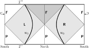
Figure 8: The worldlines of uniformly accelerated charges located symmetrically with respect to the origin (north pole) of the standard spherical coordinates in de Sitter space. The particles “start” and “end” at the equator. They are causally disconnected as a corresponding pair in Minkowski space (cf. Fig. 1). The “oriented” value $a_{\mathrm{o}}$ of the acceleration of these particles is positive (cf. the “rotated” version of Eq. (54)).

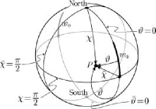
Figure 9: The rotated spherical coordinates ${\bar{\chi},\,\bar{\vartheta}}$ on 3-sphere (the cut ${\varphi=\text{constant}}$). The relation between the coordinates is given in Eq. (55).

In the classical Born solutions both charges are, at all times, located symmetrically with respect to the origin of the Minkowski coordinates (see Fig. 1). In order to demonstrate explicitly that a limiting procedure exists in which our generalized Born’s solution goes over to its classical counterpart, we shall now construct the pair of uniformly accelerated particles which are, at all times, symmetrically located with respect to the origin of the standard spherical coordinates in de Sitter space, i.e., with respect to the “north pole” at ${\chi=0}$. Asymptotically at ${\tau\to-\infty}$ these two particles both start (“are born”) with the same speed at the equator, ${\chi=\pi/2}$, at the antipodal points ${\vartheta=0}$ and ${\vartheta=\pi}$. As the universe contracts, they both move symmetrically along the axis ${\vartheta=0,\pi}$, reach some limiting value $\chi_{\mathrm{o}}$ at the moment of time symmetry, and accelerate back towards the equator, reaching the initial positions asymptotically at ${\tau\to+\infty}$. These two particles are illustrated in Fig. 8, with their worldlines denoted by $w_{\scriptscriptstyle{\oplus}}$ and $w_{\scriptscriptstyle{\ominus}}$. In Fig. 9, a snapshot at ${\tau=\text{constant}}$ is depicted. Comparing Fig. 8 with Fig. 7, it is evident that the particles $w_{\scriptscriptstyle{\oplus}}$ and $w_{\scriptscriptstyle{\ominus}}$ are located with respect to the point ${\chi=\pi/2}$, ${\vartheta=0}$ in exactly the same manner as the particles $w_{\scriptscriptstyle{\odot}}$ and $w_{\scriptscriptstyle{\otimes}}$ are located with respect to the pole ${\chi=0}$ (or, rather, as the particles $w_{\scriptscriptstyle{\odot}}^{\prime}$, $w_{\scriptscriptstyle{\otimes}}^{\prime}$, since we chose $w_{\scriptscriptstyle{\oplus}}$, $w_{\scriptscriptstyle{\ominus}}$ to have positive $a_{\mathrm{o}}$ in Fig. 8).

Owing to the global homogeneity of de Sitter space and the spherical geometry of its slices ${\tau=\text{constant}}$, the worldlines of the particles $w_{\scriptscriptstyle{\oplus}}$ and $w_{\scriptscriptstyle{\ominus}}$ can be constructed by a suitable rotation of the worldlines of the particles $w_{\scriptscriptstyle{\odot}}$ and $w_{\scriptscriptstyle{\otimes}}$. In Section VII the same rotation will be applied to obtain the fields of these particles “born at the equator.” We rotate the coordinates ${\chi,\,\vartheta,\,\varphi}$ into new coordinates ${\bar{\chi},\,\bar{\vartheta},\,\bar{\varphi}}$ which, as a pole, have the point ${\chi=\pi/2}$, ${\vartheta=0}$ (see Fig. 9). The relations between these coordinates follow from the spherical geometry:

$$\cos\bar{\chi}=\sin\chi\cos\vartheta{\mbox{\;,\quad}}\tan\bar{\vartheta}=-\tan\chi\sin\vartheta{\mbox{\;,\quad}}\bar{\varphi}=\varphi{\mbox{\;.}}$$ (55)

The new worldlines, $w_{\scriptscriptstyle{\oplus}}$ and $w_{\scriptscriptstyle{\ominus}}$, will then be given by Eqs. (40) in which ${\chi,\,\vartheta,\,\varphi}$ are replaced by rotated coordinates ${\bar{\chi},\,\bar{\vartheta},\,\bar{\varphi}}$. Substituting for these by using relations (55), we find the worldlines $w_{\scriptscriptstyle{\oplus}}$, $w_{\scriptscriptstyle{\ominus}}$ in the original coordinates to be described by the expressions:

$$\tau =\ell_{\scriptscriptstyle\Lambda}\,\operatorname{arcsinh}\Biggl{(}\frac{\sinh\bigl{(}(\cosh\alpha_{\mathrm{o}})\,{\lambda_{\scriptscriptstyle{\mathrm{dS}}}}/\ell_{\scriptscriptstyle\Lambda}\bigr{)}}{\cosh\alpha_{\mathrm{o}}}\Biggr{)}{\mbox{\;,}}$$ (56)

$$\chi =\pm\arctan\Biggl{(}-\frac{\cosh\bigl{(}(\cosh\alpha_{\mathrm{o}})\,{\lambda_{\scriptscriptstyle{\mathrm{dS}}}}/\ell_{\scriptscriptstyle\Lambda}\bigr{)}}{\sinh\alpha_{\mathrm{o}}}\Biggr{)}{\mbox{\;,}}$$

$$\vartheta =0{\mbox{\;,}}$$

with the values of $\arctan$ from ${(0,\pi)}$ and upper (lower) sign corresponding to the particle starting at the positive (negative) value of $\chi$, i.e., to the particle $w_{\scriptscriptstyle{\oplus}}$ (or $w_{\scriptscriptstyle{\ominus}}$, respectively).

Excluding the proper time $\lambda_{\scriptscriptstyle{\mathrm{dS}}}$, we arrive at simple result (cf. Eq. (44))

$$\cos\chi=-\frac{\tanh\alpha_{\mathrm{o}}}{\cosh(\tau/\ell_{\scriptscriptstyle\Lambda})}{\mbox{\;.}}$$ (57)

As ${\tau\to\pm\infty}$, then indeed ${\left\lvert\chi\right\rvert\to\pi/2}$; at ${\tau=0}$, ${\left\lvert\chi\right\rvert=\arccos(-\tanh\alpha_{\mathrm{o}})=\arccos(-R_{\mathrm{o}}/\ell_{\scriptscriptstyle\Lambda})}$, in agreement with the “deviation” of the “original” particles $w_{\scriptscriptstyle{\odot}}$, $w_{\scriptscriptstyle{\otimes}}$ from ${\chi=0}$ at ${\tau=0}$. In the spherical rescaled coordinates, Eqs. (56) read

$${\tilde{t}} =\operatorname{arccot}\Bigl{(}-\frac{\sinh\bigl{(}(\cosh\alpha_{\mathrm{o}})\,{\lambda_{\scriptscriptstyle{\mathrm{dS}}}}/\ell_{\scriptscriptstyle\Lambda}\bigr{)}}{\cosh\alpha_{\mathrm{o}}}\Bigr{)}{\mbox{\;,}}$$ (58)

$${\tilde{r}} =\pm\arctan\Bigl{(}-\frac{\cosh\bigl{(}(\cosh\alpha_{\mathrm{o}})\,{\lambda_{\scriptscriptstyle{\mathrm{dS}}}}/\ell_{\scriptscriptstyle\Lambda}\bigr{)}}{\sinh\alpha_{\mathrm{o}}}\Bigr{)}{\mbox{\;,}}$$

$$\vartheta =0{\mbox{\;,}}$$

again with the values of $\arctan$ and $\operatorname{arccot}$ from ${(0,\pi)}$. Eq. (57) becomes

$$\cos{\tilde{r}}=-{\tanh\alpha_{\mathrm{o}}}{\sin{\tilde{t}}}{\mbox{\;.}}$$ (59)

Although the flat (rescaled) cosmological coordinates cover only parts of the worldlines $w_{\scriptscriptstyle{\oplus}}$, $w_{\scriptscriptstyle{\ominus}}$ (see Figs. 8 and 3), we transcribe the equations above also into these frames in which the particles “emerge” at ${{\check{\tau}},\,{\check{t}}\to-\infty}$ at the cosmological horizon at ${{\check{r}}=\pm\infty}$. We find

$$\frac{{\check{\tau}}}{\ell_{\scriptscriptstyle\Lambda}} =-\log\biggl{(}\frac{-\cosh\alpha_{\mathrm{o}}}{-\sinh\bigl{(}(\cosh\alpha_{\mathrm{o}})\,{\lambda_{\scriptscriptstyle{\mathrm{dS}}}}/\ell_{\scriptscriptstyle\Lambda}\bigr{)}+\sinh\alpha_{\mathrm{o}}}\biggr{)}{\mbox{\;,}}$$

$$\frac{{\check{t}}}{\ell_{\scriptscriptstyle\Lambda}} =\frac{\cosh\alpha_{\mathrm{o}}}{-\sinh\bigl{(}(\cosh\alpha_{\mathrm{o}})\,{\lambda_{\scriptscriptstyle{\mathrm{dS}}}}/\ell_{\scriptscriptstyle\Lambda}\bigr{)}+\sinh\alpha_{\mathrm{o}}}{\mbox{\;,}}$$ (60)

$$\frac{{\check{r}}}{\ell_{\scriptscriptstyle\Lambda}} =\mp\frac{\cosh\bigl{(}(\cosh\alpha_{\mathrm{o}})\,{\lambda_{\scriptscriptstyle{\mathrm{dS}}}}/\ell_{\scriptscriptstyle\Lambda}\bigr{)}}{-\sinh\bigl{(}(\cosh\alpha_{\mathrm{o}})\,{\lambda_{\scriptscriptstyle{\mathrm{dS}}}}/\ell_{\scriptscriptstyle\Lambda}\bigr{)}+\sinh\alpha_{\mathrm{o}}}{\mbox{\;,}}$$

so that Eq. (59) translates into the relations

$$\begin{gathered}{\check{r}}=\pm\sqrt{\ell_{\scriptscriptstyle\Lambda}^{2}+{\check{t}}^{2}-2\,\ell_{\scriptscriptstyle\Lambda}{\check{t}}\tanh\alpha_{\mathrm{o}}}{\mbox{\;,}}\\ {\check{r}}=\pm\ell_{\scriptscriptstyle\Lambda}\sqrt{1+2\tanh\alpha_{\mathrm{o}}\,\exp(-{\check{\tau}}/\ell_{\scriptscriptstyle\Lambda})+\exp(-2{\check{\tau}}/\ell_{\scriptscriptstyle\Lambda})}{\mbox{\;.}}\end{gathered}$$ (61)

As ${{\check{\tau}}\to+\infty}$, we have ${{\check{r}}\to\pm\ell_{\scriptscriptstyle\Lambda}}$, as it corresponds to ${\chi\to\pm\pi/2}$; at ${{\check{\tau}}\to-\infty}$, we get ${{\check{r}}\to\pm\infty}$—here the particles enter flat cosmological frame at the horizon (cf. Fig. 8).

The worldlines $w_{\scriptscriptstyle{\oplus}}$, $w_{\scriptscriptstyle{\ominus}}$ are situated outside the regions covered by our choice of the hyperbolic cosmological coordinates. Similarly, we get only finite parts of $w_{\scriptscriptstyle{\oplus}}$, $w_{\scriptscriptstyle{\ominus}}$ in our static coordinates. Of course, we could rotate the static coordinates to cover both particles but then we arrive at exactly the same picture as with the particles $w_{\scriptscriptstyle{\odot}}$, $w_{\scriptscriptstyle{\otimes}}$ considered above.

Our primary reason to discuss the pair $w_{\scriptscriptstyle{\oplus}}$, $w_{\scriptscriptstyle{\ominus}}$ is to demonstrate explicitly how our fields go over into the classical Born solution in the limit of vanishing $\Lambda$. For this purpose, it will be important to have available also the description of the worldlines $w_{\scriptscriptstyle{\oplus}}$, $w_{\scriptscriptstyle{\ominus}}$ in the Minkowski coordinates introduced in Eqs. (30). As it is obvious from Fig. 6, these coordinates cover both worldlines $w_{\scriptscriptstyle{\oplus}}$ and $w_{\scriptscriptstyle{\ominus}}$ completely. Using the relations inverse to Eqs. (30) given in the Appendix, Eq. (151), we find Eqs. (58) to imply

$$t=b_{\mathrm{o}}\sinh\frac{\lambda_{\scriptscriptstyle{\mathrm{M}}}}{b_{\mathrm{o}}}{\mbox{\;,\quad}}r=\pm b_{\mathrm{o}}\cosh\frac{\lambda_{\scriptscriptstyle{\mathrm{M}}}}{b_{\mathrm{o}}}{\mbox{\;,\quad}}\vartheta=0{\mbox{\;,}}$$ (62)

where

$$\frac{b_{\mathrm{o}}}{\ell_{\scriptscriptstyle\Lambda}}=\exp\alpha_{\mathrm{o}}=\sqrt{1+a_{\mathrm{o}}^{2}\ell_{\scriptscriptstyle\Lambda}^{-2}}-a_{\mathrm{o}}\ell_{\scriptscriptstyle\Lambda}=\sqrt{\frac{\ell_{\scriptscriptstyle\Lambda}+R_{\mathrm{o}}}{\ell_{\scriptscriptstyle\Lambda}-R_{\mathrm{o}}}}{\mbox{\;,}}$$ (63)

and $\lambda_{\scriptscriptstyle{\mathrm{M}}}$ is the proper time measured in Minkowski space $M$ related to de Sitter space by conformal mapping (31), (32):

$$\lambda_{\scriptscriptstyle{\mathrm{M}}}=\exp\alpha_{\mathrm{o}}\,\cosh\alpha_{\mathrm{o}}\;\lambda_{\scriptscriptstyle{\mathrm{dS}}}{\mbox{\;.}}$$ (64)

Consequently,

$$r=\pm\sqrt{t^{2}+b_{\mathrm{o}}^{2}}{\mbox{\;,\quad}}\vartheta=0{\mbox{\;,}}$$ (65)

which is the simplest form of the hyperbolic motion with the uniform acceleration $1/b_{\mathrm{o}}$ as measured in Minkowski space (cf. Eqs. (3)).

V Frames centered on accelerated particles

For the investigation of the radiative properties and other physical aspects of the fields, the use of (physically equivalent) particles $w_{\scriptscriptstyle{\odot}}$, $w_{\scriptscriptstyle{\otimes}}$, i.e., those “born at the poles” of spherical coordinates is technically more advantageous. We shall now return back and construct frames with the origins located directly on these particles. In such frames, various properties of the fields will become more transparent than in the coordinates introduced so far.

As we have seen in the preceding section, the uniformly accelerated particles ${w_{\scriptscriptstyle{\odot}}}$ and ${w_{\scriptscriptstyle{\otimes}}}$ are at rest in static coordinates ${T,\,R}$ at given ${R=R_{\mathrm{o}}=-a_{\mathrm{o}}\ell_{\scriptscriptstyle\Lambda}^{2}/\sqrt{1+a_{\mathrm{o}}^{2}\ell_{\scriptscriptstyle\Lambda}^{2}}}$, where ${\left\lvert a_{\mathrm{o}}\right\rvert}$ is the magnitude of the acceleration. In order to investigate the properties of the fields, in particular, in order to see what is the structure of the field along the null cones with vertices at the particle’s position, i.e., what is the field “emitted” by the particle at a given time, it is useful to construct coordinate frames centered on the accelerated particles. Such systems of coordinates are used to describe accelerating black holes in general relativity (like C-metrics, known also for ${\Lambda\neq 0}$, cf. Krtouš and Podolský (2003); Podolský et al. (2003)), so that their properties on de Sitter background may indicate what is their meaning in more general cases—in situations when they are centered on gravitating objects rather than on test particles.

We shall now describe three coordinate systems of this type: the accelerated coordinates, the C-metric-like coordinates, and the Robinson-Trautman coordinates, all centered on the worldlines ${w_{\scriptscriptstyle{\odot}}}$ and ${w_{\scriptscriptstyle{\otimes}}}$. Instead of writing down just the transformation formulas, we wish to indicate some steps how these coordinates can be obtained naturally. We list only the main transformation relations here, many other formulas and forms of the metrics can be found in the Appendix. Let us also note that in this section we assume $R_{\mathrm{o}},\,\alpha_{\mathrm{o}}>0$, i.e., ${a_{\mathrm{o}}<0}$, and we use only static radial coordinate with positive values, i.e., ${R>0}$.

V.1 Accelerated coordinates

We begin with the construction of accelerated coordinates ${{T^{\prime}}{},\,{R^{\prime}}{},\,{\vartheta^{\prime}},\,\varphi}$. This type of coordinates was recently introduced Podolský and Griffiths (2001) by another method in the context of the C-metric with ${\Lambda>0}$. In the preceding section we obtained the worldlines ${w_{\scriptscriptstyle{\odot}}}$, ${w_{\scriptscriptstyle{\otimes}}}$ of uniformly accelerated particles in de Sitter space by starting from a particle moving with a uniform velocity ${v_{\scriptscriptstyle{\mathrm{\check{M}}}}=\tanh\alpha_{\mathrm{o}}}$ in a negative direction of the ${{\check{z}}}$ axis in the inertial frame ${{\check{t}},\,{\check{r}},\,\vartheta,\,\varphi}$ in Minkowski space ${\check{M}}$ which passes through ${{\check{r}}=0}$ at ${{\check{t}}=0}$ (see Eqs. (34), (35)); and we used then the conformal relation between Minkowski and de Sitter spaces to find ${w_{\scriptscriptstyle{\odot}}}$, ${w_{\scriptscriptstyle{\otimes}}}$. Therefore, let us first construct a frame centered on the uniformly moving particle in ${\check{M}}$. Using spherical coordinates again, this boosted frame denoted by primes is related to the original one simply by

$${{\check{t}}^{\prime}}{}={\check{t}}\cosh\alpha_{\mathrm{o}}+{\check{r}}\cos\vartheta\sinh\alpha_{\mathrm{o}}{\mbox{\;,}}$$ (66)

$${{\check{r}}^{\prime}}{}\cos{\vartheta^{\prime}}={\check{t}}\sinh\alpha_{\mathrm{o}}+{\check{r}}\cos\vartheta\cosh\alpha_{\mathrm{o}}{\mbox{\;,}}$$

$${{\check{r}}^{\prime}}{}\sin{\vartheta^{\prime}}={\check{r}}\sin\vartheta{\mbox{\;,}}$$

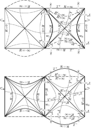
Figure 10: The 2-dimensional conformal diagrams of de Sitter space based on the static, non-accelerated coordinates (upper diagram), and on the accelerated coordinates (lower diagram). Starting from static coordinates ${T,\,R,\,\vartheta,\,\varphi}$, one can draw the conformal diagram of the axis ${\vartheta=0,\pi}$ in which the conformal past and future infinities, ${{\mathcal{I}}^{\pm}}$ (${R=\pm\infty}$), are horizontal (double) lines. In addition to static coordinates ${T,\,R}$, also accelerated coordinates ${{T^{\prime}}{},\,{R^{\prime}}{}}$ are indicated in both diagrams. These have a coordinate singularity for ${{R^{\prime}}{}=\infty}$ (drawn as a dashed line). The origins of the accelerated coordinates, ${{R^{\prime}}{}=0}$ (thick lines), are worldlines of uniformly accelerated particles. In the conformal diagram of the axis ${{\vartheta^{\prime}}=0,\pi}$ based on accelerated coordinates, the origins ${{R^{\prime}}{}=0}$ and the coordinate singularity ${{R^{\prime}}{}=\infty}$ of the accelerated frame are straight lines; the true infinities ${\mathcal{I}}^{\pm}$ have a “bulge” upwards or “downwards”, depending on the angle ${\vartheta^{\prime}}$. The hypersurface ${{R^{\prime}}{}=\infty}$ corresponds to the boosted hyperplane ${{\check{t}}^{\prime}}{}=0$, whereas the conformal infinity corresponds to ${\check{t}}=0$ (the relation of both hyperplanes can be well understood in the diagram of the conformally related Minkowski space $\check{M}$). The diagrams in which the conformal infinities ${\mathcal{I}}^{\pm}$ are not straight naturally arise in the studies of the C-metric with ${\Lambda>0}$ (de Sitter space being a special case of this class of the metrics)—see Krtouš and Podolský (2003). In general, outside the axis ${\vartheta={\vartheta^{\prime}}=0,\pi}$, the transformations between the static and accelerated coordinates mix radial and angular coordinates ${R,\vartheta}$ and ${{R^{\prime}}{},{\vartheta^{\prime}}}$, as is seen also in the following Fig. 11. The sections ${{\vartheta^{\prime}}=\text{constant}}$ (for some general ${{\vartheta^{\prime}}}$) are also shown in Fig. 21 in the Appendix.

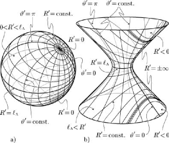
Figure 11: The accelerated coordinates ${{R^{\prime}}{},\,{\vartheta^{\prime}}}$ on the sections ${{T^{\prime}}{}=\text{constant}}$ of de Sitter space (coordinate ${\varphi}$ suppressed). In the region where ${{{\partial}/{\partial{T^{\prime}}{}}}}$ is timelike (${0<{R^{\prime}}{}<\ell_{\scriptscriptstyle\Lambda}}$), the cut ${{T^{\prime}}{}=\text{constant}}$ is a spacelike sphere (diagram a). In the region where ${{{\partial}/{\partial{T^{\prime}}{}}}}$ is spacelike (${\ell_{\scriptscriptstyle\Lambda}<{R^{\prime}}{}}$ and ${{R^{\prime}}{}<0}$), it is a timelike hyperboloid (diagram b). The diagrams are not in the same scale—the radius of the sphere and of the neck of the hyperboloid should be the same. The axis ${{\vartheta^{\prime}}=0,\pi}$ corresponds to the lines ${{T^{\prime}}{}=\text{constant}}$ of Fig. 10. The coordinate singularity ${{R^{\prime}}{}=\pm\infty}$ is also indicated. For more details see the text.

the ${\varphi}$-coordinate does not change and will be suppressed in the following. From here

$$\begin{gathered}-{{\check{t}}^{\prime}}{}^{2}+{{\check{r}}^{\prime}}{}^{2}=-{\check{t}}^{2}+{\check{r}}^{2}{\mbox{\;,}}\\ \tan{\vartheta^{\prime}}=\frac{\sin\vartheta}{({\check{t}}/{\check{r}})\sinh\alpha_{\mathrm{o}}+\cos\vartheta\cosh\alpha_{\mathrm{o}}}{\mbox{\;.}}\end{gathered}$$ (67)

The original frame ${{\check{t}},\,{\check{r}},\vartheta}$ in Minkowski space ${\check{M}}$ is related to the static coordinates ${T,\,R,\vartheta}$ in de Sitter space by (cf. Eqs. (201), (214))

$$T=-\frac{\ell_{\scriptscriptstyle\Lambda}}{2}\log\Bigl{\lvert}\frac{{\check{t}}^{2}-{\check{r}}^{2}}{\ell_{\scriptscriptstyle\Lambda}^{2}}\Bigr{\rvert}{\mbox{\;,\quad}}R=-\ell_{\scriptscriptstyle\Lambda}\frac{{\check{r}}}{{\check{t}}}{\mbox{\;,\quad}}\vartheta=\vartheta{\mbox{\;.}}$$ (68)

The metrics of the two spaces are related by ${g_{\scriptscriptstyle{\mathrm{dS}}}=(\ell_{\scriptscriptstyle\Lambda}^{2}/{\check{t}}^{2}){\mathrm{\mathit{g}}}_{\scriptscriptstyle{\mathrm{\check{M}}}}}$, ${{\mathrm{\mathit{g}}}_{\scriptscriptstyle{\mathrm{dS}}}}$ being given by Eq. (22)—cf. Eq. (27). Now, let us introduce coordinates ${{T^{\prime}}{},\,{R^{\prime}}{},\,{\vartheta^{\prime}}}$ given in terms of ${{{\check{t}}^{\prime}}{},\,{{\check{r}}^{\prime}}{},\,{\vartheta^{\prime}}}$ by exactly the same formulas as coordinates ${T,\,R,\,\vartheta}$ are given in terms of ${{\check{t}},\,{\check{r}},\,\vartheta}$ in Eq. (68). In this way we obtain ${{\mathrm{\mathit{g}}}_{{\scriptscriptstyle{\mathrm{dS}}}^{\prime}}=(\ell_{\scriptscriptstyle\Lambda}^{2}/{{\check{t}}^{\prime}}{}^{2}){\mathrm{\mathit{g}}}_{{\scriptscriptstyle{\mathrm{\check{M}}}}}}$. Combining the last relation with ${g_{\scriptscriptstyle{\mathrm{dS}}}=(\ell_{\scriptscriptstyle\Lambda}^{2}/{\check{t}}^{2}){\mathrm{\mathit{g}}}_{\scriptscriptstyle{\mathrm{\check{M}}}}}$, we find the metric of the original de Sitter space in the new coordinates ${{T^{\prime}}{},\,{R^{\prime}}{},\,{\vartheta^{\prime}}}$ in the form

$${\mathrm{\mathit{g}}}_{\scriptscriptstyle{\mathrm{dS}}}=\frac{{{\check{t}}^{\prime}}{}^{2}}{{\check{t}}^{2}}\,{\mathrm{\mathit{g}}}_{{\scriptscriptstyle{\mathrm{dS}}}^{\prime}}{\mbox{\;,}}$$ (69)

${{\mathrm{\mathit{g}}}_{{\scriptscriptstyle{\mathrm{dS}}}^{\prime}}}$ is given by the “primed” version of Eq. (22). Expressing then the factor ${({{\check{t}}^{\prime}}{}/{\check{t}})^{2}}$ by using Eqs. (66), (67), and “primed” relations (68), we arrive at the de Sitter metric in the accelerated coordinates in the form

$$\begin{split}{\mathrm{\mathit{g}}}_{\scriptscriptstyle{\mathrm{dS}}}=\,&\frac{1-{R_{\mathrm{o}}^{2}}/{\ell_{\scriptscriptstyle\Lambda}^{2}}}{\bigl{[}1+({{R^{\prime}}{}R_{\mathrm{o}}}/{\ell_{\scriptscriptstyle\Lambda}^{2}})\,\cos{\vartheta^{\prime}}\bigr{]}^{2}}\Biggl{(}-\Bigl{(}1-\frac{{R^{\prime}}{}^{2}}{\ell_{\scriptscriptstyle\Lambda}^{2}}\Bigr{)}\,{\mathrm{\mathrm{d}}}{T^{\prime}}{}{}^{2}\\ &\;+\Bigl{(}1-\frac{{R^{\prime}}{}^{2}}{\ell_{\scriptscriptstyle\Lambda}^{2}}\Bigr{)}^{\!\!-1}\!{\mathrm{\mathrm{d}}}{R^{\prime}}{}{}^{2}+{R^{\prime}}{}^{2}\,\bigl{(}{\mathrm{\mathrm{d}}}{\vartheta^{\prime}}{}^{2}+\sin^{2}{\vartheta^{\prime}}\,{\mathrm{\mathrm{d}}}\varphi{}^{2}\bigr{)}\Biggr{)}{\mbox{\;.}}\\ \end{split}$$ (70)

Here the accelerated coordinates ${{T^{\prime}}{},\,{R^{\prime}}{},\,{\vartheta^{\prime}},\,\varphi}$ are given in terms of static coordinates by the relation obtained by the procedure described above as follows:

$$\begin{gathered}{R^{\prime}}{}=\ell_{\scriptscriptstyle\Lambda}\sqrt{1-\frac{\bigl{(}1-{R^{2}}/{\ell_{\scriptscriptstyle\Lambda}^{2}}\bigr{)}\bigl{(}1-{R_{\mathrm{o}}^{2}}/{\ell_{\scriptscriptstyle\Lambda}^{2}}\bigr{)}}{\bigl{[}1-({RR_{\mathrm{o}}}/{\ell_{\scriptscriptstyle\Lambda}^{2}})\,\cos\vartheta\bigr{]}^{2}}}{\mbox{\;,}}\\ {T^{\prime}}{}=T{\mbox{\;,\quad}}\tan{\vartheta^{\prime}}=\frac{\sqrt{1-{R_{\mathrm{o}}^{2}}/{\ell_{\scriptscriptstyle\Lambda}^{2}}}\;R\sin\vartheta}{R\cos\vartheta-R_{\mathrm{o}}}{\mbox{\;.}}\end{gathered}$$ (71)

Notice that the time coordinate of static and accelerated frames coincide. Technically, this is easy to see from the first relation in Eqs. (67) and Eq. (68). Intuitively, this is evident since the uniformly accelerated particles are at rest in the static coordinates, as well as in the accelerated coordinates, the only difference being that they are located at the origin of the accelerated frame. Setting ${R_{\mathrm{o}}=0}$ in Eq. (71), we get ${{R^{\prime}}{}=R}$, ${{\vartheta^{\prime}}=\vartheta}$, as expected. The static coordinates are centered on the poles ${\chi=0,\,\pi}$, hence, on the unaccelerated worldlines. The name accelerated coordinates is thus inspired by the fact that their origin is accelerated, and the value of this acceleration enters the form of the metric (70) explicitly through the quantity ${R_{\mathrm{o}}}$.

The 2-dimensional conformal diagram of de Sitter space with coordinate lines ${{T^{\prime}}{}=\text{constant}}$, ${{R^{\prime}}{}=\text{constant}}$ of the accelerated frame is given in Fig. 10. For details, see the figure caption. Here let us just notice that the cosmological horizons are still described by ${{R^{\prime}}{}^{2}=\ell_{\scriptscriptstyle\Lambda}^{2}}$. Infinite values of ${{R^{\prime}}{}}$ can, however, be encountered “before” the conformal infinities ${\mathcal{I}}^{\pm}$ are reached. This depends on the angle ${\vartheta^{\prime}}$. Indeed, ${R^{\prime}}{}=\infty$ corresponds to ${{\check{t}}^{\prime}}{}=0$, whereas ${\mathcal{I}}^{\pm}$ is given by ${\check{t}}=0$, i.e.,

$${R^{\prime}}{}=-\frac{\ell_{\scriptscriptstyle\Lambda}^{2}}{R_{\mathrm{o}}}\frac{1}{\cos{\vartheta^{\prime}}}{\mbox{\;,}}$$ (72)

(cf. metric (70)). Relation of these two surfaces is best viewed in Minkowski space ${\check{M}}$. We see that for ${\vartheta,{\vartheta^{\prime}}<\pi/2}$, the conformal infinity ${\mathcal{I}}^{+}$ (${\mathcal{I}}^{-}$) lies “above” (“below”) the surface ${{R^{\prime}}{}=\pm\infty}$. Thus the infinity ${{R^{\prime}}{}=\pm\infty}$ is just a coordinate singularity, which can be removed using, for example, the C-metric-like coordinate $\upsilon$ introduced below.

Fig. 11a shows the cut ${T={T^{\prime}}{}=\text{constant}}$ located in the region of de Sitter space where the Killing vector ${{\partial}/{\partial T}}={{\partial}/{\partial{T^{\prime}}{}}}$ is timelike (${R,{R^{\prime}}{}<\ell_{\scriptscriptstyle\Lambda}}$); $\varphi$-direction is suppressed. The cut is a spacelike sphere $S^{3}$ with homogeneous spherical metric. The coordinate lines ${{R^{\prime}}{}=\text{constant}}$ and ${{\vartheta^{\prime}}=\text{constant}}$ are plotted, with two origins ${{R^{\prime}}{}=0}$ indicated: here the accelerated particles occur. The coordinate ${R^{\prime}}{}$ grows from ${R^{\prime}}{}=0$ at the origins to the equator where ${{R^{\prime}}{}=\ell_{\scriptscriptstyle\Lambda}}$. In Fig. 11b the cut ${T={T^{\prime}}{}=\text{constant}}$ located in the regions where ${{\partial}/{\partial T}}={{\partial}/{\partial{T^{\prime}}{}}}$ is spacelike (${R,{R^{\prime}}{}>\ell_{\scriptscriptstyle\Lambda}}$) is illustrated, again with $\varphi$-direction suppressed. Here the cut is timelike with the geometry of three-dimensional de Sitter space. The coordinate lines ${{R^{\prime}}{}=\text{constant}}$ and ${{\vartheta^{\prime}}=\text{constant}}$ are also shown.

As we have just seen, the points with ${{R^{\prime}}{}=\infty}$ can be “nice” points in de Sitter manifold. It may thus be convenient to introduce the inverse of ${R^{\prime}}{}$ as a new coordinate. Also, we consider ${-\cos{\vartheta^{\prime}}}$ as a new coordinate, and make the time coordinate dimensionless. We thus arrive at the C-metric-like coordinates ${\tau,\,\upsilon,\,\xi,\,\varphi}$:

$$\tau=\frac{{T^{\prime}}{}}{\ell_{\scriptscriptstyle\Lambda}}{\mbox{\;,\quad}}\upsilon=\frac{\ell_{\scriptscriptstyle\Lambda}}{{R^{\prime}}{}}{\mbox{\;,\quad}}\xi=-\cos{\vartheta^{\prime}}{\mbox{\;.}}$$ (73)

The metric (70) becomes

$$\begin{split}{\mathrm{\mathit{g}}}_{\scriptscriptstyle{\mathrm{dS}}}={\mathfrak{r}}^{2}\,&\Bigl{(}-(\upsilon^{2}-1)\,{\mathrm{\mathrm{d}}}\tau{}^{2}+\frac{1}{\upsilon^{2}-1}\,{\mathrm{\mathrm{d}}}\upsilon{}^{2}\\ &\qquad\quad+\frac{1}{1-\xi^{2}}\,{\mathrm{\mathrm{d}}}\xi{}^{2}+(1-\xi^{2})\,{\mathrm{\mathrm{d}}}\varphi{}^{2}\Bigr{)}{\mbox{\;,}}\end{split}$$ (74)

with the conformal factor ${\mathfrak{r}}$ given by

$${\mathfrak{r}}=\frac{\ell_{\scriptscriptstyle\Lambda}}{\upsilon\cosh\alpha_{\mathrm{o}}-\xi\sinh\alpha_{\mathrm{o}}}{\mbox{\;.}}$$ (75)

This is de Sitter spacetime in the “C-metric form”: setting the mass and charge parameters, ${m}$ and ${e}$, equal to zero in the the C-metric with a positive cosmological constant (written in the form (2.8) of Ref. Krtouš and Podolský (2003)), and choosing the acceleration parameter equal to ${A=\ell_{\scriptscriptstyle\Lambda}^{-1}\left\lvert\sinh\alpha_{\mathrm{o}}\right\rvert=\left\lvert a_{\mathrm{o}}\right\rvert}$, we obtain the metric (74).

V.2 Robinson-Trautman coordinates

In order to arrive naturally to the Robinson-Trautman form of the metric, notice that the coefficients in the metric (74) become singular at ${\upsilon\to\pm 1}$, similarly as they do on the horizon of the Schwarzschild spacetime in the standard Schwarzschild coordinates. Analogously to that case, we choose a “tortoise-type” coordinate $\upsilon_{\star}$ by

$$\upsilon_{\star}=\frac{1}{2}\log\left\lvert\frac{1-\upsilon}{1+\upsilon}\right\rvert{\mbox{\;.}}$$ (76)

Similarly to the Schwarzschild case again, we introduce a suitable null coordinate ${\mathfrak{u}}$ in terms of the radial and time coordinates $\tau$ and $\upsilon_{\star}$ as follows:

$${\mathfrak{u}}=(\ell_{\scriptscriptstyle\Lambda}\tanh\alpha_{\mathrm{o}})\,(\tau+\upsilon_{\star}){\mbox{\;.}}$$ (77)

Together with the conformal factor ${\mathfrak{r}}$ defined in Eq. (75), we arrive at the de Sitter metric in coordinates ${{\mathfrak{u}},\,{\mathfrak{r}},\,\xi,\,\varphi}$ (cf. Eq. (243)) which is very near to being in the Robinson-Trautman form. However, there is a non-vanishing mixed metric coefficient at ${{\mathrm{\mathrm{d}}}{\mathfrak{u}}\mathbin{\scriptstyle{\vee}}{\mathrm{\mathrm{d}}}\xi}$ which is absent in the Robinson-Trautman metric. Such a term can be made to vanish by introducing a new angular coordinate $\psi$ by

$$\psi=\operatorname{arctanh}\xi+\frac{{\mathfrak{u}}}{\ell_{\scriptscriptstyle\Lambda}}\,\sinh\alpha_{\mathrm{o}}{\mbox{\;.}}$$ (78)

The de Sitter metric then becomes

$${\mathrm{\mathit{g}}}_{\scriptscriptstyle{\mathrm{dS}}}=-H\,{\mathrm{\mathrm{d}}}{\mathfrak{u}}{}^{2}-{\mathrm{\mathrm{d}}}{\mathfrak{u}}\mathbin{\scriptstyle{\vee}}{\mathrm{\mathrm{d}}}{\mathfrak{r}}+\frac{{\mathfrak{r}}^{2}}{P^{2}}\,\bigl{(}{\mathrm{\mathrm{d}}}\psi{}^{2}+{\mathrm{\mathrm{d}}}\varphi{}^{2}\bigr{)}{\mbox{\;,}}$$ (79)

where

$$H=-\frac{{\mathfrak{r}}^{2}}{\ell_{\scriptscriptstyle\Lambda}^{2}}+2\,\frac{{\mathfrak{r}}}{\ell_{\scriptscriptstyle\Lambda}}\,\sinh\alpha_{\mathrm{o}}\,\tanh\Bigl{(}\psi-\frac{{\mathfrak{u}}}{\ell_{\scriptscriptstyle\Lambda}}\,\sinh\alpha_{\mathrm{o}}\Bigr{)}+1{\mbox{\;,}}$$

$$P=\cosh\Bigl{(}\psi-\frac{{\mathfrak{u}}}{\ell_{\scriptscriptstyle\Lambda}}\,\sinh\alpha_{\mathrm{o}}\Bigr{)}{\mbox{\;.}}$$ (80)

This is precisely the form of the Robinson-Trautman metric—see, e.g., Stephani et al. (2002). Tracking back the transformations leading to the metric (79), the connection between the Robinson-Trautman coordinates and the static coordinates ${T,\,R,\,\vartheta,\,\varphi}$ turns out to be not as complicated as our procedure might have indicated, in particular, for the radial coordinate. We find a nice formula for ${{\mathfrak{r}}}$,

$${\mathfrak{r}}=\frac{\ell_{\scriptscriptstyle\Lambda}}{\sqrt{1-\frac{R_{\mathrm{o}}^{2}}{\ell_{\scriptscriptstyle\Lambda}^{2}}}}\,\Biggl{(}\Bigl{(}1-\frac{RR_{\mathrm{o}}}{\ell_{\scriptscriptstyle\Lambda}^{2}}\cos\vartheta\Bigr{)}^{2}-\Bigl{(}1-\frac{R^{2}}{\ell_{\scriptscriptstyle\Lambda}^{2}}\Bigr{)}\Bigl{(}1-\frac{R_{\mathrm{o}}^{2}}{\ell_{\scriptscriptstyle\Lambda}^{2}}\Bigr{)}\Biggr{)}^{\frac{1}{2}}\!\!\!{\mbox{\;,}}$$ (81)

whereas the other two coordinates are simply expressed only in terms of accelerated coordinates ${{T^{\prime}}{}=T,\,{R^{\prime}}{},\,{\vartheta^{\prime}},\,\varphi}$:

$${\mathfrak{u}} =\sqrt{1-\frac{R_{\mathrm{o}}^{2}}{\ell_{\scriptscriptstyle\Lambda}^{2}}}\,\Biggl{(}{T^{\prime}}{}+\frac{\ell_{\scriptscriptstyle\Lambda}}{2}\log\left\lvert\frac{{R^{\prime}}{}-\ell_{\scriptscriptstyle\Lambda}}{{R^{\prime}}{}+\ell_{\scriptscriptstyle\Lambda}}\right\rvert\Biggr{)}{\mbox{\;,}}$$ (82)

$$\psi =\frac{R_{\mathrm{o}}}{\ell_{\scriptscriptstyle\Lambda}}\,\Biggl{(}\frac{{T^{\prime}}{}}{\ell_{\scriptscriptstyle\Lambda}}+\frac{1}{2}\log\left\lvert\frac{{R^{\prime}}{}-\ell_{\scriptscriptstyle\Lambda}}{{R^{\prime}}{}+\ell_{\scriptscriptstyle\Lambda}}\right\rvert\Biggr{)}+\log\left\lvert\tan\frac{{\vartheta^{\prime}}}{2}\right\rvert{\mbox{\;.}}$$

Coordinates ${{R^{\prime}}{},\,{\vartheta^{\prime}}}$ can then be obtained in terms of the original static coordinates by using Eqs. (71).

The Robinson-Trautman coordinates with metric (79) are centered on the accelerated particles. As with static or accelerated frames, we need two sets of such coordinates to cover both $w_{\scriptscriptstyle{\odot}}$ and $w_{\scriptscriptstyle{\otimes}}$. The relations to the static coordinates become, of course, much simpler if the particles are not accelerated, ${R_{\mathrm{o}}=0}$, and when both the Robinson-Trautman and static coordinates are centered on the pole ${\chi=0}$:

$$\begin{gathered}{\mathfrak{r}}=R{\mbox{\;,\quad}}\psi=\log\tan\frac{\vartheta}{2}{\mbox{\;,}}\\ {\mathfrak{u}}=T+\frac{\ell_{\scriptscriptstyle\Lambda}}{2}\,\log\left\lvert\frac{R-\ell_{\scriptscriptstyle\Lambda}}{R+\ell_{\scriptscriptstyle\Lambda}}\right\rvert{\mbox{\;.}}\end{gathered}$$ (83)

However, even “accelerated” Robinson-Trautman coordinates possess some very convenient features. The radial coordinate ${\mathfrak{r}}$ is an affine parameter along null rays ${{\mathfrak{u}},\,\psi,\,\varphi=\text{constants}}$, normalized at the particle’s worldline by the condition

$${\frac{\partial^{\mu}}{\partial{\mathfrak{r}}}}\,{\mathrm{\mathit{g}}}_{{\scriptscriptstyle{\mathrm{dS}}}\mu\nu}\,{\mathrm{u}}^{\nu}=-1{\mbox{\;,}}$$ (84)

where ${{\mathrm{u}}}$ is the particle’s four-velocity. These null rays form a diverging but nonshearing and nonrotating congruence of geodesics. The null vector ${{{\partial}/{\partial{\mathfrak{r}}}}}$, tangent to the rays, is parallelly propagated along them. Its divergence is given by ${\nabla_{\mu}{\frac{\partial^{\mu}}{\partial{\mathfrak{r}}}}=2/{\mathfrak{r}}}$ so that ${\mathfrak{r}}$ is both the affine parameter and the luminosity distance (see, e.g., Bondi et al. (1962)). With Robinson-Trautman coordinates, one can also associate a null tetrad (explicitly written down in the Appendix, Eq. (248)) which is parallelly transported along the null rays from the particle (${{\mathfrak{r}}=0}$) up to infinity (${{\mathfrak{r}}=\infty}$).

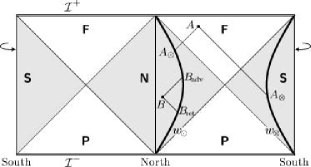
Figure 12: The field at an event ${A}$ can be interpreted as ${1/2}$ of the sum of the retarded fields produced by particle ${w_{\scriptscriptstyle{\odot}}}$ at ${A_{\scriptscriptstyle{\odot}}}$ and particle ${w_{\scriptscriptstyle{\otimes}}}$ at ${A_{\scriptscriptstyle{\otimes}}}$. The field at ${B}$ can be interpreted as ${1/2}$ of the sum of the retarded and advanced effects from particle ${w_{\scriptscriptstyle{\odot}}}$. The affine parameter distances ${BB_{\scriptscriptstyle{\mathrm{ret}}}}$ and ${BB_{\scriptscriptstyle{\mathrm{adv}}}}$ are equal, the same being true for the distances ${AA_{\scriptscriptstyle{\odot}}}$ and ${AA_{\scriptscriptstyle{\otimes}}}$.

Owing to the boost symmetry of both the worldlines and de Sitter space, an interesting feature arises, which is analogous to the situation in Minkowski space. Consider a point ${B}$ in region N (Fig. 12). There are two generators of the null cone with the origin at ${B}$ which cross the worldline ${w_{\scriptscriptstyle{\odot}}}$ at two points, ${B_{\scriptscriptstyle{\mathrm{ret}}}}$ and ${B_{\scriptscriptstyle{\mathrm{adv}}}}$. Then the affine parameter distance ${BB_{\scriptscriptstyle{\mathrm{ret}}}}$ is the same as ${BB_{\scriptscriptstyle{\mathrm{adv}}}}$. (In order to go towards the past from ${B_{\scriptscriptstyle{\mathrm{adv}}}}$ to ${B}$, the “advanced” Robinson-Trautman coordinates built on the past null cones with origins on ${w_{\scriptscriptstyle{\odot}}}$ can easily be introduced.) This is evident because ${B}$ lies on one orbit of the boost Killing vector ${{{\partial}/{\partial T}}}$ and a boost can be applied which leaves the worldline ${w_{\scriptscriptstyle{\odot}}}$ invariant but moves ${B}$ into event ${B^{\prime}}$ on the slice of time symmetry, ${\tau=0}$ (also ${T={T^{\prime}}{}=0}$), where the particle is at rest. Then ${B_{\scriptscriptstyle{\mathrm{adv}}}}$ and ${B_{\scriptscriptstyle{\mathrm{ret}}}}$ move to the new points ${B^{\prime}_{\scriptscriptstyle{\mathrm{adv}}}}$, ${B^{\prime}_{\scriptscriptstyle{\mathrm{ret}}}}$, which are located symmetrically with respect to ${\tau=0}$. The equality of the affine parameter distances then follows from the symmetry immediately. Similarly, for an event ${A}$ in region F one can show that the affine parameter distance ${AA_{\scriptscriptstyle{\odot}}}$ is equal to the distance ${AA_{\scriptscriptstyle{\otimes}}}$ (see Fig. 12). The point ${A}$ lies on a boost orbit (which now has a spatial character) along which it can be brought, by an appropriate boost, to the point located symmetrically between the worldlines ${w_{\scriptscriptstyle{\odot}}}$ and ${w_{\scriptscriptstyle{\otimes}}}$ (lying so on the equator, ${\chi=\pi/2}$). The same consideration can, of course, be applied to an event in the “past” region P—showing that the affine distances along future-oriented null rays from an event to the particles are equal.

Although the symmetries just described are common to the worldlines of uniformly accelerated particles in Minkowski and de Sitter spacetimes, an important difference exists. In Minkowski space, the affine parameter distance along the null ray from an event on particle’s worldline, such as ${A_{\scriptscriptstyle{\odot}}}$, to an “observation” point ${A}$ is equal to the proper distance between ${A_{\perp}}$ and ${A_{\scriptscriptstyle{\odot}}}$ where ${A_{\perp}}$ is the orthogonal projection of ${A}$ onto the spacelike slice ${T=T(A_{\scriptscriptstyle{\odot}})}$. This is not the case in de Sitter space if, as it appears natural, under an ‘orthogonal projection’ we understand the projection of the observation point ${A}$ onto the spacelike slice ${T=\text{constant}}$ containing ${A_{\scriptscriptstyle{\odot}}}$ performed along a timelike geodesic orthogonal to such a slice. Nevertheless, the proper distance $s$ between ${A_{\scriptscriptstyle{\odot}}}$ and ${A_{\perp}}$ is still related to the affine parameter distance ${\mathfrak{r}}$ by a simple expression:

$$\frac{{\mathfrak{r}}}{\ell_{\scriptscriptstyle\Lambda}}=\tan\frac{s}{\ell_{\scriptscriptstyle\Lambda}}{\mbox{\;.}}$$ (85)

This relation can be derived as follows. Consider, without loss of generality, ${A_{\scriptscriptstyle{\odot}}}$ located at the turning point of the particle ${w_{\scriptscriptstyle{\odot}}}$ at ${T=0}$. The condition that the events $A$ and ${A_{\scriptscriptstyle{\odot}}}$ are connected by a null ray implies that the distance $s$ between ${A_{\scriptscriptstyle{\odot}}}$ and ${A_{\perp}}$ is the same as the time interval between ${A_{\perp}}$ and $A$ as measured by the metric (25) of the conformally related static Einstein universe. Since $A$ occurs at some time ${\tilde{t}}$ whereas $A_{\scriptscriptstyle{\odot}}$ and $A_{\perp}$ at ${{\tilde{t}}=\pi/2}$ (i.e., at static time ${T=0}$), this time interval is equal to ${\ell_{\scriptscriptstyle\Lambda}({\tilde{t}}-\pi/2)}$, cf. Eq. (24). The static radial coordinate $R$ of $A$ thus reads (cf. Eqs. (198), (211))

$$R=\frac{\sin{\tilde{r}}}{\sin{\tilde{t}}}=\frac{\sin{\tilde{r}}}{\cos(s/\ell_{\scriptscriptstyle\Lambda})}{\mbox{\;.}}$$ (86)

The slice ${T=0}$ has a geometry of the 3-sphere of radius $\ell_{\scriptscriptstyle\Lambda}$. Using the standard law of cosines in spherical trigonometry for the sides of the triangle spanned by $A_{\scriptscriptstyle{\odot}}$, $A_{\perp}$, and the north pole, we can eliminate ${\tilde{r}}$. Finally, employing Eq. (81), we obtain the result (85). Clearly, near the particle ${w_{\scriptscriptstyle{\odot}}}$ we have ${s\ll\ell_{\scriptscriptstyle\Lambda}}$, and Eq. (85) then gives ${{\mathfrak{r}}\approx s}$, as in Minkowski space.

In the following section we shall explore the character of the fields of the particles ${w_{\scriptscriptstyle{\odot}}}$ and ${w_{\scriptscriptstyle{\otimes}}}$. We shall see that the affine parameter distance ${{\mathfrak{r}}}$ will play most important role, simplifying their description enormously. Namely, as we will see in Section VI.2, Eq. (114), the affine parameter ${{\mathfrak{r}}}$ is identical to the factor ${{\mathcal{Q}}}$ which will be introduced in the following and will appear in all expressions for the fields.

VI Fields of uniformly accelerated sources and their many faces

In this section we wish to construct the scalar and electromagnetic fields of uniformly accelerated (scalar and electric) charges in de Sitter universe. A general procedure, suitable in case of any—not necessarily uniform—acceleration would be to seek for appropriate Green’s functions. Alternatively, in particular for sources moving along uniformly accelerated worldlines, we can make use of the conformal relations between Minkowski and de Sitter spaces, and of the properties of scalar and electromagnetic fields under conformal mappings. This method is advantageous not only for finding the fields in de Sitter spacetime, but also for understanding their relationships to the known fields of corresponding sources in special relativity. The only delicate issue is the fact that there are no conformal mappings between Minkowski and de Sitter space which are globally smooth. We discussed, in Section III, how various regions of one space can be mapped onto the regions of the other space. In Ref. Bičák and Krtouš (2001) we carefully treated the fields at the hypersurfaces where the conformal transformation fails to be regular. In order to obtain well-behaved fields, one must continue analytically across such a hypersuface the field obtained in one region into the whole de Sitter space. In Section II in Ref. Bičák and Krtouš (2001), we also analyzed in detail the behavior of the scalar field wave equation with sources and of Maxwell’s equations with sources under (general) conformal transformations.

In Ref. Bičák and Krtouš (2001) we primarily concentrated on the absence of purely retarded fields at the past infinity ${\mathcal{I}}^{-}$ of de Sitter spacetime—in fact, in any spacetime in which ${\mathcal{I}}^{-}$ is spacelike. In order to analyze this problem we also considered, in addition to monopole charges, more complicated sources like rigid and geodesic dipoles; and we constructed some retarded solutions to show their patological features. However, we confined ourselves to the sources the worldlines of which start and end at the poles; we did not employ coordinates best suited for exhibiting the properties of the fields at future infinity ${\mathcal{I}}^{+}$, and the frames corresponding to cosmological models like flat ($k=0$) or hyperbolic ($k=-1$) cosmological coordinates; and we did not give the physical components of the fields. In the following we shall find the fields and discuss their properties in various physically important coordinate systems, in particular those significant at ${\mathcal{I}}^{+}$ or in a cosmological context. In the next section, we also obtain the fields due to the uniformly accelerated scalar and electric charges starting at ${\mathcal{I}}^{-}$ at ${\chi=\pi/2}$ (“born at the equator”). This, among others, will be important when we wish to regain the classical Born fields in the limit ${\Lambda\to 0}$.

We start by using the analysis of the conformal behavior of the fields and sources given in Section II in Bičák and Krtouš (2001), and we also take over from Bičák and Krtouš (2001) the resulting forms of the fields due to the sources starting and ending at the poles of de Sitter space, as described in standard coordinates.

VI.1 Fields in coordinates centered on the poles

Consider two uniformly accelerated point sources starting at ${\mathcal{I}}^{-}$ (i.e., at ${\tau\to-\infty}$, ${{\tilde{t}}\to 0}$) at the poles ${\chi={\tilde{r}}=0}$ and ${\chi={\tilde{r}}=\pi}$ (Fig. 7). Their worldlines $w_{\scriptscriptstyle{\odot}}$, $w_{\scriptscriptstyle{\otimes}}$ are given by Eqs. (40) (or (58)) in these standard (rescaled) coordinates, by Eqs. (41) and (42) in the flat and hyperbolic cosmological coordinates, and by Eqs. (52) in the static coordinates. Their simplest description is, of course, given by ${{R^{\prime}}{}=0}$ and ${{\mathfrak{r}}=0}$ in the accelerated and Robinson-Trautman coordinates since these frames are centered exactly on their worldlines. In Section IV we discussed physical velocities and other properties of these particles.

Now, as noticed at the beginning of Section IV, these two worldlines can be obtained by conformally mapping the worldline of one uniformly moving particle in Minkowski space into de Sitter space. The fields of uniformly moving sources in Minkowski space are just boosted Coulomb fields. Under a conformal rescaling of the metric, ${{\mathrm{\mathit{g}}}_{\alpha\beta}\to\hat{\mathrm{\mathit{g}}}_{\alpha\beta}=\Omega^{2}{\mathrm{\mathit{g}}}_{\alpha\beta}}$, the fields behave as follows: ${\Phi\to\hat{\Phi}=\Omega^{-1}\Phi}$, ${{\mathrm{F}}_{\alpha\beta}\to\hat{{\mathrm{F}}}_{\alpha\beta}={\mathrm{F}}_{\alpha\beta}}$ (see Bičák and Krtouš (2001), Section II, where the behavior of the source terms is also analyzed). Hence, the fields due to two uniformly accelerated sources in de Sitter spacetime can be obtained by conformally transforming the boosted Coulomb fields in Minkowski spacetime. Employing the conformal mapping (26)–(28), we arrive at the following results (note nt: ). The scalar field is given by the expression

$$\Phi=\frac{s}{4\pi}\frac{1}{{\mathcal{Q}}}{\mbox{\;,}}$$ (87)

where

$$\begin{split}{\mathcal{Q}}&=\ell_{\scriptscriptstyle\Lambda}\Bigl{[}\Bigl{(}\sqrt{1\!+\!a_{\mathrm{o}}^{2}\ell_{\scriptscriptstyle\Lambda}^{2}}+a_{\mathrm{o}}\ell_{\scriptscriptstyle\Lambda}\cosh\frac{\tau}{\ell_{\scriptscriptstyle\Lambda}}\sin\chi\cos\vartheta\Bigr{)}^{2}\\ &\mspace{120.0mu}-\Bigl{(}1-\cosh^{2}\frac{\tau}{\ell_{\scriptscriptstyle\Lambda}}\,\sin^{2}\chi\Bigr{)}\Bigr{]}^{\frac{1}{2}}{\mbox{\;,}}\end{split}$$ (88)

or, written in the standard rescaled coordinates,

$${\mathcal{Q}}=\ell_{\scriptscriptstyle\Lambda}\Bigl{[}\!\Bigl{(}\sqrt{1\!+\!a_{\mathrm{o}}^{2}\ell_{\scriptscriptstyle\Lambda}^{2}}+a_{\mathrm{o}}\ell_{\scriptscriptstyle\Lambda}\frac{\sin{\tilde{r}}}{\sin{\tilde{t}}}\cos\vartheta\Bigr{)}^{\!2}\!-1+\frac{\sin^{2}{\tilde{r}}}{\sin^{2}{\tilde{t}}}\Bigr{]}^{\frac{1}{2}}\!{\mbox{\;.}}$$ (89)

This field is produced by two identical charges of magnitude $s$ moving along worldlines $w_{\scriptscriptstyle{\odot}}$ and $w_{\scriptscriptstyle{\otimes}}$. It is smooth everywhere outside the charges and it can be written as a symmetric combination of retarded and advanced effects from both charges (cf. Eq. (6.6) in Bičák and Krtouš (2001)).

Similarly to the scalar-field case, by using conformal technique the electromagnetic field produced by two uniformly accelerated charges moving along $w_{\scriptscriptstyle{\odot}}$ and $w_{\scriptscriptstyle{\otimes}}$ can be obtained in the form

$$\begin{split}{\mathrm{F}}=&\frac{e}{4\pi}\,\frac{\ell_{\scriptscriptstyle\Lambda}^{2}}{{\mathcal{Q}}^{3}}\cosh\frac{\tau}{\ell_{\scriptscriptstyle\Lambda}}\,\Bigl{[}\,a_{\mathrm{o}}\ell_{\scriptscriptstyle\Lambda}\sin\chi\cos\chi\sin\vartheta\,{\mathrm{\mathrm{d}}}\tau\wedge{\mathrm{\mathrm{d}}}\vartheta\\ &\;-\!\Bigl{(}\!\sqrt{1\!+a_{\mathrm{o}}^{\,2}\ell_{\scriptscriptstyle\Lambda}^{2}}\cosh\frac{\tau}{\ell_{\scriptscriptstyle\Lambda}}\sin\chi\!+a_{\mathrm{o}}\ell_{\scriptscriptstyle\Lambda}\cos\vartheta\Bigr{)}\,{\mathrm{\mathrm{d}}}\tau\wedge{\mathrm{\mathrm{d}}}\chi\\ &\;+a_{\mathrm{o}}\ell_{\scriptscriptstyle\Lambda}^{2}\sinh\frac{\tau}{\ell_{\scriptscriptstyle\Lambda}}\cosh\frac{\tau}{\ell_{\scriptscriptstyle\Lambda}}\sin^{2}\chi\sin\vartheta\,{\mathrm{\mathrm{d}}}\chi\wedge{\mathrm{\mathrm{d}}}\vartheta\,\Bigr{]}{\mbox{\;,}}\end{split}$$ (90)

where ${\mathcal{Q}}$ is again given by Eq. (88). As in the scalar-field case, the field is smooth, non-vanishing in the whole de Sitter spacetime and involving thus both retarded and advanced effects (cf. Section VIIA in Bičák and Krtouš (2001)). However, an important difference between the scalar and electromagnetic case exists: the magnitude of the scalar charges is the same, whereas the electromagnetic charges producing the fields (90) have opposite signs. This is analogous to the situation in Minkowski spacetime described in Section II (see the discussion below Eq. (13)). At the root of this fact appears to be CPT theorem—cf. Bičák (1968) for the analogous gravitational case where the masses of the particles uniformly accelerated in the opposite direction are the same. In de Sitter spacetime, as in any spacetime with compact spacelike sections, a simpler argument exists: the total charge in a compact space must vanish as a consequence of the Gauss theorem Bičák and Krtouš (2001).

To gain a better physical insight into the electromagnetic fields, we shall introduce the orthonormal tetrad ${\{{{\mathrm{e}}_{\mu}}\}}$ and the dual tetrad ${\{{{\mathrm{e}}^{\mu}}}\}$ tied to each coordinate frame used, and we shall decompose the electromagnetic field ${\mathrm{F}}$ into the electric and magnetic parts. Such a decomposition, of course, depends on the choice of the tetrad. For example, in the standard spherical coordinates ${\tau,\,\chi,\,\vartheta,\,\varphi}$ the electromagnetic field (2-form) ${\mathrm{F}}$ can be written as

$$\begin{split}{\mathrm{F}}&={\mathrm{E}}^{\chi}\,{{\mathrm{e}}^{\chi}}\wedge{{\mathrm{e}}^{\tau}}+{\mathrm{E}}^{\vartheta}\,{{\mathrm{e}}^{\vartheta}}\wedge{{\mathrm{e}}^{\tau}}+{\mathrm{E}}^{\varphi}\,{{\mathrm{e}}^{\varphi}}\wedge{{\mathrm{e}}^{\tau}}\\ &+{\mathrm{B}}^{\chi}\,{{\mathrm{e}}^{\vartheta}}\wedge{{\mathrm{e}}^{\varphi}}+{\mathrm{B}}^{\vartheta}\,{{\mathrm{e}}^{\varphi}}\wedge{{\mathrm{e}}^{\chi}}+{\mathrm{B}}^{\varphi}\,{{\mathrm{e}}^{\chi}}\wedge{{\mathrm{e}}^{\vartheta}}{\mbox{\;,}}\end{split}$$ (91)

and the electric and magnetic field spatial vectors are given in terms of their frame components as follows:

$$\begin{split}{\mathrm{E}}&={\mathrm{E}}^{\chi}\,{{\mathrm{e}}_{\chi}}+{\mathrm{E}}^{\vartheta}\,{{\mathrm{e}}_{\vartheta}}+{\mathrm{E}}^{\varphi}\,{{\mathrm{e}}_{\varphi}}{\mbox{\;,}}\\ {\mathrm{B}}&={\mathrm{B}}^{\chi}\,{{\mathrm{e}}_{\chi}}+{\mathrm{B}}^{\vartheta}\,{{\mathrm{e}}_{\vartheta}}+{\mathrm{B}}^{\varphi}\,{{\mathrm{e}}_{\varphi}}{\mbox{\;.}}\end{split}$$ (92)

In the present case of the standard spherical coordinates, using the explicit forms of the tetrad given in the Appendix (Eqs. (144)), we find

$${\mathrm{E}}_{{\scriptscriptstyle{\mathrm{sph}}}}=\frac{e}{4\pi}\frac{\ell_{\scriptscriptstyle\Lambda}}{{\mathcal{Q}}^{3}}\Bigl{[}-a_{\mathrm{o}}\ell_{\scriptscriptstyle\Lambda}\cos\chi\sin\vartheta\;{{\mathrm{e}}_{\vartheta}}$$

$$\mspace{40.0mu}+\Bigl{(}\sqrt{1+a_{\mathrm{o}}^{\,2}\ell_{\scriptscriptstyle\Lambda}^{2}}\,\cosh\frac{\tau}{\ell_{\scriptscriptstyle\Lambda}}\,\sin\chi+a_{\mathrm{o}}\ell_{\scriptscriptstyle\Lambda}\cos\vartheta\Bigr{)}\,{{\mathrm{e}}_{\chi}}\Bigr{]}{\mbox{\;,}}$$

$${\mathrm{B}}_{{\scriptscriptstyle{\mathrm{sph}}}}=\frac{e}{4\pi}\,\frac{a_{\mathrm{o}}\ell_{\scriptscriptstyle\Lambda}^{2}}{{\mathcal{Q}}^{3}}\;\sinh\frac{\tau}{\ell_{\scriptscriptstyle\Lambda}}\,\sin\chi\sin\vartheta\;{{\mathrm{e}}_{\varphi}}{\mbox{\;.}}$$ (93)

In the Appendix the orthonormal tetrads tied to the coordinate systems considered in this paper are all listed explicitly. The only exception is the Robinson-Trautman coordinate system with one coordinate null and thus with a nondiagonal metric; in this case the null tetrad is given in which the Newman-Penrose-type components are more telling.

The tetrad components of the electric intensity and the magnetic induction vectors are physically meaningful objects: they can be measured by observers who move with the four-velocities given by the timelike vector of the tetrad (as, e.g., ${{\mathrm{e}}_{\tau}}$ for spherical cosmological observers), and are equipped with an orthonormal triad of the spacelike vectors (e.g., ${{{\mathrm{e}}_{\chi}},\,{{\mathrm{e}}_{\vartheta}},\,{{\mathrm{e}}_{\varphi}}}$).

We first list the resulting electromagnetic field tensor and its electric and magnetic parts in the coordinate systems centered on the poles ${\chi=0,\pi}$. The scalar field is always given by expression (87), the explicit form of the scalar factor ${\mathcal{Q}}$ changes according to the coordinates used. Since this factor enters all the electromagnetic quantities as well, we always give ${\mathcal{Q}}$ first and then write the electromagnetic field quantities.

In the flat cosmological coordinates (see Eqs. (17), (18)) we find:

$$\begin{split}{\mathcal{Q}}&=\ell_{\scriptscriptstyle\Lambda}\Bigl{[}\Bigl{(}\cosh\alpha_{\mathrm{o}}-\sinh\alpha_{\mathrm{o}}\,\frac{{\check{r}}}{\ell_{\scriptscriptstyle\Lambda}}\,\exp\frac{{\check{\tau}}}{\ell_{\scriptscriptstyle\Lambda}}\,\cos\vartheta\Bigr{)}^{2}\\ &\mspace{140.0mu}-\Bigl{(}1-\frac{{\check{r}}^{2}}{\ell_{\scriptscriptstyle\Lambda}^{2}}\,\exp\Bigl{(}2\frac{{\check{\tau}}}{\ell_{\scriptscriptstyle\Lambda}}\Bigr{)}\Bigr{)}\Bigr{]}^{\frac{1}{2}}{\mbox{\;,}}\end{split}$$ (94)

$$\begin{split}{\mathrm{F}}&=-\frac{e}{4\pi}\,\frac{1}{{\mathcal{Q}}^{3}}\,\exp\frac{{\check{\tau}}}{\ell_{\scriptscriptstyle\Lambda}}\,\Bigl{[}\,\ell_{\scriptscriptstyle\Lambda}{\check{r}}\,\sinh\alpha_{\mathrm{o}}\,\sin\vartheta\,{\mathrm{\mathrm{d}}}{\check{\tau}}\wedge{\mathrm{\mathrm{d}}}\vartheta\\ &\quad+\Bigl{(}{\check{r}}\,\cosh\alpha_{\mathrm{o}}\,\exp\frac{{\check{\tau}}}{\ell_{\scriptscriptstyle\Lambda}}-\ell_{\scriptscriptstyle\Lambda}\sinh\alpha_{\mathrm{o}}\,\cos\vartheta\Bigr{)}\,{\mathrm{\mathrm{d}}}{\check{\tau}}\wedge{\mathrm{\mathrm{d}}}{\check{r}}\\ &\quad+{\check{r}}^{2}\,\sinh\alpha_{\mathrm{o}}\,\exp\Bigl{(}2\frac{{\check{\tau}}}{\ell_{\scriptscriptstyle\Lambda}}\Bigr{)}\sin\vartheta\,{\mathrm{\mathrm{d}}}{\check{r}}\wedge{\mathrm{\mathrm{d}}}\vartheta\,\Bigr{]}{\mbox{\;,}}\end{split}$$ (95)

$${\mathrm{E}}_{{\scriptscriptstyle{\mathrm{flat}}}} =\frac{e}{4\pi}\frac{\ell_{\scriptscriptstyle\Lambda}}{{\mathcal{Q}}^{3}}\Bigl{[}\,\sinh\alpha_{\mathrm{o}}\;\sin\vartheta\;{{\mathrm{e}}_{\vartheta}}$$ (96)

$$\mspace{15.0mu}-\!\Bigl{(}\cosh\alpha_{\mathrm{o}}\frac{{\check{r}}}{\ell_{\scriptscriptstyle\Lambda}}\exp\frac{{\check{\tau}}}{\ell_{\scriptscriptstyle\Lambda}}-\sinh\alpha_{\mathrm{o}}\cos\vartheta\Bigr{)}\,{{\mathrm{e}}_{{\check{r}}}}\Bigr{]}{\mbox{\;,}}$$

$${\mathrm{B}}_{{\scriptscriptstyle{\mathrm{flat}}}} =-\frac{e}{4\pi}\,\frac{\ell_{\scriptscriptstyle\Lambda}\sinh\alpha_{\mathrm{o}}}{{\mathcal{Q}}^{3}}\,\frac{{\check{r}}}{\ell_{\scriptscriptstyle\Lambda}}\,\exp\frac{{\check{\tau}}}{\ell_{\scriptscriptstyle\Lambda}}\,\sin\vartheta\;{{\mathrm{e}}_{\varphi}}{\mbox{\;.}}$$

In the hyperbolic cosmological coordinates (see Eqs. (19), (20)), the results are slightly lengthier:

$$\begin{split}{\mathcal{Q}}&=\ell_{\scriptscriptstyle\Lambda}\Bigl{[}\Bigl{(}\cosh\alpha_{\mathrm{o}}-\sinh\alpha_{\mathrm{o}}\,\sinh\frac{\eta}{\ell_{\scriptscriptstyle\Lambda}}\,\sinh\frac{\rho}{\ell_{\scriptscriptstyle\Lambda}}\,\cos\vartheta\Bigr{)}^{2}\\ &\mspace{100.0mu}-\Bigl{(}1-\sinh^{2}\frac{\eta}{\ell_{\scriptscriptstyle\Lambda}}\,\sinh^{2}\frac{\rho}{\ell_{\scriptscriptstyle\Lambda}}\Bigr{)}\Bigr{]}^{\frac{1}{2}}{\mbox{\;,}}\end{split}$$ (97)

$$\begin{split}{\mathrm{F}}&=-\frac{e}{4\pi}\,\frac{\ell_{\scriptscriptstyle\Lambda}}{{\mathcal{Q}}^{3}}\,\Bigl{[}\;\sinh\frac{\eta}{\ell_{\scriptscriptstyle\Lambda}}\\ &\;\times\!\!\bigl{(}\cosh\alpha_{\mathrm{o}}\,\sinh\frac{\eta}{\ell_{\scriptscriptstyle\Lambda}}\,\sinh\frac{\rho}{\ell_{\scriptscriptstyle\Lambda}}-\sinh\alpha_{\mathrm{o}}\,\cos\vartheta\bigr{)}\,{\mathrm{\mathrm{d}}}\eta\wedge{\mathrm{\mathrm{d}}}\rho\\ &\;+\sinh\alpha_{\mathrm{o}}\,\sinh\frac{\eta}{\ell_{\scriptscriptstyle\Lambda}}\,\sinh\frac{\rho}{\ell_{\scriptscriptstyle\Lambda}}\,\cosh\frac{\rho}{\ell_{\scriptscriptstyle\Lambda}}\,\sin\vartheta\,\ell_{\scriptscriptstyle\Lambda}{\mathrm{\mathrm{d}}}\eta\wedge{\mathrm{\mathrm{d}}}\vartheta\\ &\;+\sinh\alpha_{\mathrm{o}}\,\sinh^{2}\frac{\eta}{\ell_{\scriptscriptstyle\Lambda}}\,\cosh\frac{\eta}{\ell_{\scriptscriptstyle\Lambda}}\,\sinh^{2}\frac{\rho}{\ell_{\scriptscriptstyle\Lambda}}\,\sin\vartheta\,\ell_{\scriptscriptstyle\Lambda}{\mathrm{\mathrm{d}}}\rho\wedge{\mathrm{\mathrm{d}}}\vartheta\Bigr{]}\!{\mbox{\;,}}\end{split}$$ (98)

$${\mathrm{E}}_{{\scriptscriptstyle{\mathrm{hyp}}}}=\frac{e}{4\pi}\frac{\ell_{\scriptscriptstyle\Lambda}}{{\mathcal{Q}}^{3}}\Bigl{[}\,\sinh\alpha_{\mathrm{o}}\,\cosh\frac{\rho}{\ell_{\scriptscriptstyle\Lambda}}\sin\vartheta\,{{\mathrm{e}}_{\vartheta}}$$

$$\qquad\quad+\bigl{(}\cosh\alpha_{\mathrm{o}}\,\sinh\frac{\eta}{\ell_{\scriptscriptstyle\Lambda}}\,\sinh\frac{\rho}{\ell_{\scriptscriptstyle\Lambda}}-\sinh\alpha_{\mathrm{o}}\,\cos\vartheta\bigr{)}\,{{\mathrm{e}}_{\rho}}\Bigr{]}{\mbox{\;,}}$$

$${\mathrm{B}}_{{\scriptscriptstyle{\mathrm{hyp}}}}=-\frac{e}{4\pi}\frac{\ell_{\scriptscriptstyle\Lambda}}{{\mathcal{Q}}^{3}}\sinh\alpha_{\mathrm{o}}\cosh\frac{\eta}{\ell_{\scriptscriptstyle\Lambda}}\sinh\frac{\rho}{\ell_{\scriptscriptstyle\Lambda}}\sin\vartheta\;{{\mathrm{e}}_{\varphi}}{\mbox{\;.}}$$ (99)

Much simpler expressions for the fields arise in the static coordinates (see Eqs. (21), (22)). We obtain

$${\mathcal{Q}}^{2}=\frac{(\ell_{\scriptscriptstyle\Lambda}^{2}-RR_{\mathrm{o}}\cos\vartheta)^{2}}{(\ell_{\scriptscriptstyle\Lambda}^{2}-R_{\mathrm{o}}^{2})}-(\ell_{\scriptscriptstyle\Lambda}^{2}-R^{2}){\mbox{\;,}}$$ (100)

$$\begin{split}{\mathrm{F}}=&-\frac{e}{4\pi}\,\frac{\ell_{\scriptscriptstyle\Lambda}}{\sqrt{\ell_{\scriptscriptstyle\Lambda}^{2}-R_{\mathrm{o}}^{2}}}\,\frac{1}{{\mathcal{Q}}^{3}}\;\biggl{[}(R-R_{\mathrm{o}}\cos\vartheta)\;{\mathrm{\mathrm{d}}}T\wedge{\mathrm{\mathrm{d}}}R\\ &\mspace{50.0mu}+\Bigl{(}1-\frac{R^{2}}{\ell_{\scriptscriptstyle\Lambda}^{2}}\Bigr{)}RR_{\mathrm{o}}\sin\vartheta\;{\mathrm{\mathrm{d}}}T\wedge{\mathrm{\mathrm{d}}}\vartheta\biggr{]}{\mbox{\;,}}\end{split}$$ (101)

$${\mathrm{E}}_{{\scriptscriptstyle{\mathrm{stat}}}}=\frac{e}{4\pi}\,\frac{1}{{\mathcal{Q}}^{3}}\biggl{[}\frac{\ell_{\scriptscriptstyle\Lambda}(R-R_{\mathrm{o}}\cos\vartheta)}{\sqrt{\ell_{\scriptscriptstyle\Lambda}^{2}-R_{\mathrm{o}}^{2}}}\;{{\mathrm{e}}_{R}}+R_{\mathrm{o}}\sin\vartheta\;{{\mathrm{e}}_{\vartheta}}\biggr{]}{\mbox{\;,}}$$

$${\mathrm{B}}_{{\scriptscriptstyle{\mathrm{stat}}}}=0{\mbox{\;.}}$$ (102)

Since for practical calculations and for an understanding of the conformal relations between Minkowski and de Sitter spaces the rescaled coordinates are very useful, we also give the fields in these coordinates. The rescaled coordinates are tied with the same orthonormal tetrad as non-rescaled ones, and they define the same splitting into electric and magnetic parts (${\mathrm{E}}$ and ${\mathrm{B}}$ are the same spatial vectors); the functional dependence on the coordinates, however, is different. In the standard rescaled (conformally Einstein) coordinates (see Eqs. (23)–(25)), which cover the whole de Sitter spacetime including its conformal infinities globally, we get Eq. (89) for ${{\mathcal{Q}}}$ and

$$\begin{split}{\mathrm{F}}=&-\frac{e}{4\pi}\,\frac{1}{{\mathcal{Q}}^{3}}\frac{\ell_{\scriptscriptstyle\Lambda}^{3}}{\sin^{3}{\tilde{t}}}\Bigl{[}\,a_{\mathrm{o}}\ell_{\scriptscriptstyle\Lambda}\cos{\tilde{t}}\sin^{2}{\tilde{r}}\sin\vartheta\,{\mathrm{\mathrm{d}}}{\tilde{r}}\wedge{\mathrm{\mathrm{d}}}\vartheta\\ &+\Bigl{(}\sqrt{1+a_{\mathrm{o}}^{\,2}\ell_{\scriptscriptstyle\Lambda}^{2}}\sin{\tilde{r}}+a_{\mathrm{o}}\ell_{\scriptscriptstyle\Lambda}\sin{\tilde{t}}\cos\vartheta\Bigr{)}\,{\mathrm{\mathrm{d}}}{\tilde{t}}\wedge{\mathrm{\mathrm{d}}}{\tilde{r}}\\ &-a_{\mathrm{o}}\ell_{\scriptscriptstyle\Lambda}\sin{\tilde{t}}\cos{\tilde{r}}\sin{\tilde{r}}\sin\vartheta\,{\mathrm{\mathrm{d}}}{\tilde{t}}\wedge{\mathrm{\mathrm{d}}}\vartheta\,\Bigr{]}{\mbox{\;,}}\end{split}$$ (103)

$${\mathrm{E}}_{{\scriptscriptstyle{\mathrm{sph}}}} =\frac{e}{4\pi}\frac{\ell_{\scriptscriptstyle\Lambda}}{{\mathcal{Q}}^{3}}\Bigl{[}-a_{\mathrm{o}}\ell_{\scriptscriptstyle\Lambda}\cos{\tilde{r}}\sin\vartheta\;{{\mathrm{e}}_{\vartheta}}$$ (104)

$$\qquad+\Bigl{(}\!\sqrt{1+a_{\mathrm{o}}^{\,2}\ell_{\scriptscriptstyle\Lambda}^{2}}\;\frac{\sin{\tilde{r}}}{\sin{\tilde{t}}}+a_{\mathrm{o}}\ell_{\scriptscriptstyle\Lambda}\cos\vartheta\Bigr{)}\,{{\mathrm{e}}_{\chi}}\Bigr{]}{\mbox{\;,}}$$

$${\mathrm{B}}_{{\scriptscriptstyle{\mathrm{sph}}}} =-\frac{e}{4\pi}\,\frac{a_{\mathrm{o}}\ell_{\scriptscriptstyle\Lambda}^{2}}{{\mathcal{Q}}^{3}}\;\cot{\tilde{t}}\sin{\tilde{r}}\sin\vartheta\;{{\mathrm{e}}_{\varphi}}{\mbox{\;,}}$$

whereas in the flat rescaled cosmological coordinates (26)–(28), which cover globally the conformally related Minkowski space (see also Fig. 3), we arrive at

$${\mathcal{Q}}=\ell_{\scriptscriptstyle\Lambda}\biggl{[}\Bigl{(}\cosh\alpha_{\mathrm{o}}+\sinh\alpha_{\mathrm{o}}\frac{{\check{r}}}{{\check{t}}}\cos\vartheta\Bigr{)}^{2}\!-\Bigl{(}1-\frac{{\check{r}}^{2}}{{\check{t}}^{2}}\Bigr{)}\biggr{]}^{\frac{1}{2}}{\mbox{\;,}}$$ (105)

$$\begin{split}{\mathrm{F}}=\,&\frac{e}{4\pi}\,\frac{1}{{\mathcal{Q}}^{3}}\frac{\ell_{\scriptscriptstyle\Lambda}^{3}}{{\check{t}}^{3}}\Bigl{[}\,\sinh\alpha_{\mathrm{o}}\;{\check{r}}^{2}\sin\vartheta\,{\mathrm{\mathrm{d}}}{\check{r}}\wedge{\mathrm{\mathrm{d}}}\vartheta\\ &\;\;+\bigl{(}\cosh\alpha_{\mathrm{o}}\;{\check{r}}+\sinh\alpha_{\mathrm{o}}\;{\check{t}}\cos\vartheta\bigr{)}\,{\mathrm{\mathrm{d}}}{\check{t}}\wedge{\mathrm{\mathrm{d}}}{\check{r}}\\ &\;\;-\sinh\alpha_{\mathrm{o}}\;{\check{t}}\,{\check{r}}\sin\vartheta\,{\mathrm{\mathrm{d}}}{\check{t}}\wedge{\mathrm{\mathrm{d}}}\vartheta\,\Bigr{]}{\mbox{\;,}}\end{split}$$ (106)

$${\mathrm{E}}_{{\scriptscriptstyle{\mathrm{flat}}}} =\frac{e}{4\pi}\frac{\ell_{\scriptscriptstyle\Lambda}}{{\mathcal{Q}}^{3}}\biggl{[}\,\sinh\alpha_{\mathrm{o}}\;\sin\vartheta\;{{\mathrm{e}}_{\vartheta}}$$ (107)

$$\qquad-\Bigl{(}\!\cosh\alpha_{\mathrm{o}}\,\frac{{\check{r}}}{{\check{t}}}+\sinh\alpha_{\mathrm{o}}\cos\vartheta\Bigr{)}\,{{\mathrm{e}}_{{\check{r}}}}\biggr{]}{\mbox{\;,}}$$

$${\mathrm{B}}_{{\scriptscriptstyle{\mathrm{flat}}}} =\frac{e}{4\pi}\,\frac{\ell_{\scriptscriptstyle\Lambda}\sinh\alpha_{\mathrm{o}}}{{\mathcal{Q}}^{3}}\,\frac{{\check{r}}}{{\check{t}}}\,\sin\vartheta\;{{\mathrm{e}}_{\varphi}}{\mbox{\;.}}$$

In various contexts the electromagnetic field four-potential form ${\mathrm{A}}$, implying the field ${{\mathrm{F}}={\mathrm{\mathrm{d}}}{\mathrm{A}}}$, may be needed. In the standard rescaled (conformally Einstein) coordinates the potential reads

$$\begin{split}\mspace{-10.0mu}{\mathrm{A}}=-\frac{e}{4\pi}\frac{1}{{\mathcal{Q}}}&\frac{\ell_{\scriptscriptstyle\Lambda}}{\sin{\tilde{t}}}\,\frac{\sqrt{1+a_{\mathrm{o}}^{\,2}\ell_{\scriptscriptstyle\Lambda}^{2}}\sin{\tilde{t}}+a_{\mathrm{o}}\ell_{\scriptscriptstyle\Lambda}\sin{\tilde{r}}\cos\vartheta}{\sin^{2}{\tilde{t}}-\sin^{2}{\tilde{r}}}\\ &\times\Bigl{(}\sin{\tilde{t}}\cos{\tilde{r}}\,{\mathrm{\mathrm{d}}}{\tilde{t}}-\cos{\tilde{t}}\sin{\tilde{r}}\,{\mathrm{\mathrm{d}}}{\tilde{r}}\Bigr{)}{\mbox{\;.}}\end{split}$$ (108)

From this expression the frame components can easily be obtained and the four-potential form can be transformed directly to any coordinate system of interest. The four-potential acquires a particularly simple form in static coordinates:

$${\mathrm{A}}=-\frac{e}{4\pi}\,\frac{1}{{\mathcal{Q}}}\;\frac{\ell_{\scriptscriptstyle\Lambda}^{2}-RR_{\mathrm{o}}\cos\vartheta}{\ell_{\scriptscriptstyle\Lambda}\sqrt{\ell_{\scriptscriptstyle\Lambda}^{2}-R_{\mathrm{o}}^{2}}}\;{\mathrm{\mathrm{d}}}T{\mbox{\;.}}$$ (109)

Inspecting now the expressions (90)–(107), we first notice few basic features of the fields. As a consequence of the axisymmetry, the azimuthal $\varphi$ component of the electric field vanishes. On the other hand, only the azimuthal $\varphi$ component of the magnetic field is non-zero. At the axis of symmetry, ${\vartheta=0,\pi}$, the latitudinal $\vartheta$ component of the electric field and magnetic field vanish as ${\sim\sin\vartheta}$. The electric field points along the axis.

In the classical Born solution in Minkowski space, both charges are, at any time, located symmetrically with respect to the equatorial plane ${\vartheta=\pi/2}$. Consequently, the radial part of the electric field vanishes for ${\vartheta=\pi/2}$ (cf. Eq. (13)). In de Sitter spacetime the charges outgoing from the poles are, at all times, symmetrically located with respect to the sphere ${\chi=\pi/2}$ (illustrated as the circle in Fig. 2). We thus expect the $\vartheta$ component of the electric field to vanish for ${\chi=\pi/2}$. This, indeed, follows from Eq. (93). This symmetry can be seen only in the standard spherical coordinates since the sphere ${\chi=\pi/2}$ is not covered by the hyperbolic cosmological coordinates and in the flat cosmological coordinates only one particle occurs.

Another typical feature of the Born solution in Minkowski space is its time symmetry. As a consequence, the magnetic field vanishes at ${t=0}$ (cf. Eq. (13)). In the past, it was this fact which led some investigators, W. Pauli Pauli (1958) among them, to the conclusion that there is “no formation of a wave zone nor any corresponding radiation” since ${{\mathrm{B}}=0}$ at ${t=0}$. However, it is not at a spacelike hypersurface ${t=\text{constant}}$ but at ${{\mathcal{I}}^{+}}$, which is reached by taking ${u=t-r}$ constant, ${t,\,r\to\infty}$, where the Born field has typical radiative features, i.e., ${\left\lvert{\mathrm{E}}\right\rvert=\left\lvert{\mathrm{B}}\right\rvert\sim r^{-1}}$ (see Fulton and Rohrlich (1960), Bičák (1968), Bičák and Krtouš (2002)). In our generalized Born solution, the time symmetry of the fields is clearly demonstrated in the global standard coordinates: under inversion ${\tau\to-\tau}$ the electric field in Eq. (93) is invariant, whereas the magnetic field changes the sign; ${{\mathrm{B}}_{\varphi}=0}$ at ${\tau=0}$. The field also exhibits radiative character when we approach ${{\mathcal{I}}^{+}}$ in an appropriate way, as it is briefly indicated in Bičák and Krtouš (2002). As mentioned in the Introduction, a detailed analysis of the radiative properties of the generalized Born field will be given elsewhere.

The fields take the simplest form in the static coordinates, Eq. (101). In these coordinates the particles are at rest, and they both have a constant distance from the poles; their world lines are the orbits of the “static” Killing vector ${{{\partial}/{\partial T}}}$ of de Sitter space. The electric field is time independent, the magnetic field vanishes. This is fully analogous to the Born field in Minkowski spacetime: it is static, and purely electric in the Rindler coordinates, the time coordinate of which is aligned along the orbit of the boost Killing vectors (see, e.g., Boulware (1980)). However, as we discussed in Section III, the static coordinates cover only a “half” of de Sitter space. In the other half, the Killing vector ${{{\partial}/{\partial T}}}$ becomes spacelike. It is in this non-static domain (regions F and P in Fig. 12) where we expect, in analogy with the results in Minkowski spacetime, to find fields which have radiative properties. ${{{\partial}/{\partial T}}}$ is the Killing vector also in the non-static regions, however, it is spacelike here, as it is typical for a boost Killing vector in Minkowski space. The fields of uniformly accelerated charges in de Sitter spacetime are invariant under the boosts along ${{{\partial}/{\partial T}}}$ everywhere. They are thus boost-rotation symmetric as the Born fields in Minkowski spacetime.

In the cosmological coordinates, respectively, in their rescaled versions, the fields are, of course, time dependent. Here we expect the effects of the expansion/contraction of de Sitter universe to be manifested. Indeed, considering in any of the cosmological frames the spatial coordinates fixed, and examining the fields along the timelike geodesics, we discover that the fields exponentially decay at large times, i.e., as ${{\mathcal{I}}^{+}}$ is approached. More specifically, with the spherical coordinates ${\chi,\,\vartheta,\,\varphi}$ fixed, the factor ${{\mathcal{Q}}}$ behaves as ${\exp(\tau/\ell_{\scriptscriptstyle\Lambda})}$ at large times ${\tau}$, and hence, we obtain ${{\mathrm{E}}_{{\scriptscriptstyle{\mathrm{sph}}}}\approx c_{1}\exp(-2\tau/\ell_{\scriptscriptstyle\Lambda}){{\mathrm{e}}_{\chi}}}{+c_{2}\exp(-3\tau/\ell_{\scriptscriptstyle\Lambda}){{\mathrm{e}}_{\vartheta}}}$, ${{\mathrm{B}}_{{\scriptscriptstyle{\mathrm{sph}}}}\approx b_{1}\exp(-2\tau/\ell_{\scriptscriptstyle\Lambda}){{\mathrm{e}}_{\varphi}}}$, ${c_{1},\,c_{2},\,b_{1}}$ being constants. The electric field thus becomes radial at large ${\tau}$. Similarly, in flat cosmological coordinates we find ${{\mathrm{E}}_{{\scriptscriptstyle{\mathrm{flat}}}}\approx c_{1}\exp(-2{\check{\tau}}/\ell_{\scriptscriptstyle\Lambda}){{\mathrm{e}}_{{\check{r}}}}}$, ${{\mathrm{B}}_{{\scriptscriptstyle{\mathrm{flat}}}}\approx b_{1}\exp(-2{\check{\tau}}/\ell_{\scriptscriptstyle\Lambda}){{\mathrm{e}}_{\varphi}}}$. In the hyperbolic cosmological coordinates the proper time ${\eta}$ appears instead of ${{\check{\tau}}}$. The rapid decay of the fields along timelike worldlines at large times is caused by the exponential expansion (at large times) of the spatial slices ${\tau=\text{constant}}$ (respectively ${{\check{\tau}},\,\eta=\text{constant}}$). Although our fields are just test fields, their exponential decay is another manifestation of the “cosmic no-hair phenomenon”: geodesic observers in spacetimes with ${\Lambda>0}$ see at large times these spacetimes to approach the de Sitter universe exponentially fast—the universe becomes “bald” (see, e.g., Maeda (1989); Rendall (2004)). Clearly, as one approaches past infinity ${{\mathcal{I}}^{-}}$ (${\tau\to-\infty}$), the fields also decay exponentially.

It is interesting to notice the character of the field as it would be seen by the observers at rest with respect to the hyperbolic cosmological coordinates in the limit at which the particles “enter” the region covered by these observers across the horizon ${{\tilde{t}}={\tilde{r}}}$ (cf. Fig. 4), given in the hyperbolic coordinates by ${\eta\to 0}$, ${\rho\to\infty}$. As discussed in Section IV, the observed velocity (51) of the charges at this boundary is (in the limit) equal to the velocity of light. Employing the transformation formulas (220), it is easy to see that at this boundary ${\left\lvert\sinh(\eta/\ell_{\scriptscriptstyle\Lambda})\,\sinh(\rho/\ell_{\scriptscriptstyle\Lambda})\right\rvert\to 1}$. Hence, the factor ${{\mathcal{Q}}}$ is finite here (as it is evident from its scalar character and its finiteness in the global standard coordinates). Also, the radial part of the electric field remains finite. However, ${{\mathrm{E}}^{\vartheta}}$ diverges as ${\exp(\rho/\ell_{\scriptscriptstyle\Lambda})}$ here, indicating that the field has a character of an impulse, in fact, rather of an impulsive wave: indeed, Eq. (96) implies ${\left\lvert{\mathrm{E}}^{\vartheta}\right\rvert=\left\lvert{\mathrm{B}}^{\varphi}\right\rvert}$. The situation appears to be analogous to the field of a static charge viewed from an inertial frame boosted to the velocity of light in Minkowski spacetime (see, e.g., Jackson (1975)).

VI.2 Fields in coordinates centered on the particles

As expected, a remarkable simplification occurs when the fields are evaluated in the coordinates at the origin of which the charges are situated at all times. Since the accelerated coordinates ${{T^{\prime}}{},\,{R^{\prime}}{},\,{\vartheta^{\prime}}}$ and the C-metric-like coordinates are simply related by Eqs. (73), the discussion of the field properties is the same in both these frames. Namely, notice that both coordinate systems are tied with the same orthonormal tetrad, and they thus define the same splitting of the field into the electric and magnetic parts. In these coordinates, we find the factor ${{\mathcal{Q}}}$ to read

$$\begin{split}{\mathcal{Q}}&=\cosh\alpha_{\mathrm{o}}\,\frac{1}{{R^{\prime}}{}}\,+\sinh\alpha_{\mathrm{o}}\,\frac{1}{\ell_{\scriptscriptstyle\Lambda}}\cos{\vartheta^{\prime}}\\ &=\frac{1}{\ell_{\scriptscriptstyle\Lambda}}\bigl{(}\upsilon\cosh\alpha_{\mathrm{o}}-\xi\sinh\alpha_{\mathrm{o}}\bigr{)}{\mbox{\;.}}\end{split}$$ (110)

The scalar field is again given by ${\Phi=(s/4\pi)\,{\mathcal{Q}}^{-1}}$, and the electromagnetic field also acquires now an extremely simple form:

$${\mathrm{F}}=\frac{e}{4\pi}\,\frac{1}{{R^{\prime}}{}^{2}}\,{\mathrm{\mathrm{d}}}{R^{\prime}}{}\wedge{\mathrm{\mathrm{d}}}{T^{\prime}}{}=\frac{e}{4\pi}\,{\mathrm{\mathrm{d}}}\tau\wedge{\mathrm{\mathrm{d}}}\upsilon{\mbox{\;,}}$$ (111)

$${\mathrm{E}}_{{\scriptscriptstyle{\mathrm{acc}}}}=\frac{e}{4\pi}\,\frac{1}{{\mathcal{Q}}^{2}}\,{{\mathrm{e}}_{{R^{\prime}}{}}}{\mbox{\;,\quad}}{\mathrm{B}}_{{\scriptscriptstyle{\mathrm{acc}}}}=0{\mbox{\;.}}$$ (112)

The magnetic field vanishes in the frame tied to the accelerated and C-metric coordinates, the electric field has precisely the Coulomb form, with the factor ${{\mathcal{Q}}}$ playing the role of a distance.

As signalized above already, the factor ${{\mathcal{Q}}}$ turns out to be the Robinson-Trautman radial coordinate (see Eq. (114) below), i.e., the affine parameter distance allong null geodesics. The geometrical role of ${{\mathcal{Q}}}$ was elucidated in Section V.2. Considering a fixed point in de Sitter universe and a light cone emanating from this point, three typical situations can arise as illustrated in Fig. 12. For a point ${B}$ from the regions N or S, there are two null geodesics, one past-pointing, the other future-pointing, each of which crosses the worldline of the same particle, say ${w_{\scriptscriptstyle{\odot}}}$ (in case of ${B}$ from N), at points ${B_{\scriptscriptstyle{\mathrm{ret}}}}$ and ${B_{\scriptscriptstyle{\mathrm{adv}}}}$ (see Fig. 12). Since ${{\mathcal{Q}}}$ is equal to the (specific) affine parameter distance which is the same from ${B_{\scriptscriptstyle{\mathrm{ret}}}}$ as from ${B_{\scriptscriptstyle{\mathrm{adv}}}}$ (see Section V.2), we can interpret the field (112) as arising from purely retarded, respectively, advanced effects from ${B_{\scriptscriptstyle{\mathrm{ret}}}}$, respectively ${B_{\scriptscriptstyle{\mathrm{adv}}}}$; or, equivalently, as a combination of retarded and advanced effects from these points. In the second situation, when the fixed point, say ${A}$, is located “above the roof” (in the region F), there are two past-oriented null geodesics emanating from it which cross now both particles ${w_{\scriptscriptstyle{\odot}}}$ and ${w_{\scriptscriptstyle{\otimes}}}$ at points ${A_{\scriptscriptstyle{\odot}}}$ and ${A_{\scriptscriptstyle{\otimes}}}$ (see Fig. 12). The field can be interpreted as arising from retarded effects only, either as a combination from both particles ${w_{\scriptscriptstyle{\odot}}}$ and ${w_{\scriptscriptstyle{\otimes}}}$, or as the retarded field from just one of them. Finally, for a point from the region P the field can analogously be interpreted in terms of advanced effects.

As we discussed in Section V.1 and illustrated in detail in the Appendix, the accelerated coordinates (similarly as the static coordinates to which they go over for a vanishing acceleration) are static, i.e., the vector ${{{\partial}/{\partial{T^{\prime}}{}}}}$ tangent to the orbits of the Killing vector is timelike, only in the regions N and S (cf. Figs. 10, 12). Observers following the orbits of the Killing vector are thus confined to the regions N and S, and they cannot detect the fields in the region F (respectively P). Nevertheless, notice that although the time coordinate ${{T^{\prime}}{}}$ diverges at the horizon ${R=\ell_{\scriptscriptstyle\Lambda}}$, the radial coordinate ${{R^{\prime}}{}}$ is perfectly finite there, ${{R^{\prime}}{}=\ell_{\scriptscriptstyle\Lambda}}$ (cf. Eq. (71) with ${R=\ell_{\scriptscriptstyle\Lambda}}$), and the field (111) is meaningful in the region F (or P) as well. Since here the roles of the coordinates ${{R^{\prime}}{}}$ and ${{T^{\prime}}{}}$ are interchanged, ${{R^{\prime}}{}}$ becoming a time coordinate, the field becomes time-dependent. As mentioned above, we do not expect to find radiative properties in the regions N and S. Indeed, in accelerated coordinates the field (112) is static Coulomb field, with ${{\mathcal{Q}}}$ playing the role of a distance. However, the radiative properties of the whole field in the wave zone in the region F are not evident from the time-dependent, purely electric field in the accelerated coordinates with ${{R^{\prime}}{}}$ as a time coordinate.

It is worthwhile to recall that with finite sources in Minkowski spacetime the field at any event is of a general algebraic type; only asymptotically, at large distances, its features approach those of a null field (${{\mathrm{E}}^{2}-{\mathrm{B}}^{2}=0}$, ${{\mathrm{E}}\mathbin{\boldsymbol{\cdot}}{\mathrm{B}}=0}$), if there is a radiation (see, e.g., Goldberg and Kerr (1964); Penrose and Rindler (1984, 1986)). In case of a non-null field, one can always introduce a frame in which the electric and magnetic fields are collinear, or, in the language of the Newman-Penrose formalism, to choose such a null tetrad ${{{\mathrm{k}}},\,{{\mathrm{l}}},\,{{\mathrm{m}}},\,{\bar{{\mathrm{m}}}}}$, corresponding to the orthonormal tetrad, that the only non-vanishing null-tetrad component is ${\Phi_{1}=\frac{1}{2\sqrt{2}}\,({\mathrm{E}}-i{\mathrm{B}})\mathbin{\boldsymbol{\cdot}}({{\mathrm{k}}}-{{\mathrm{l}}})}$ (see Eqs. (248) for the explicit expressions of the null tetrad and Eqs. (138) for the null-tetrad components of the electromagnetic field). Such a situation arises precisely for the null tetrad associated with the accelerated coordinates: the null-tetrad components are simply

$$\Phi_{1}^{{\scriptscriptstyle{\mathrm{acc}}}}=-\frac{1}{2}\,\frac{e}{4\pi}\,\frac{1}{{\mathcal{Q}}^{2}}{\mbox{\;,\quad}}\Phi_{0}^{{\scriptscriptstyle{\mathrm{acc}}}}=\Phi_{2}^{{\scriptscriptstyle{\mathrm{acc}}}}=0{\mbox{\;.}}$$ (113)

The vanishing of the other two null-tetrad components, ${\Phi_{0}^{{\scriptscriptstyle{\mathrm{acc}}}}}$ and ${\Phi_{2}^{{\scriptscriptstyle{\mathrm{acc}}}}}$, has a deeper algebraic explanation: the null tetrad tied to the accelerated coordinates is special in the sense that it contains both principal null directions of the electromagnetic field. Inspecting the form of the null tetrad constructed from the orthonormal tetrad (229), we observe that both these principal null directions are tangent to the “radial” surfaces ${{\vartheta^{\prime}},\,\varphi=\text{constant}}$ in the accelerated coordinates.

The radiative properties are well exhibited in the Robinson-Trautman coordinates. As we discussed in Section V.2, these coordinates are tied to the future null cones centered on the worldline of a particle. We consider the null cones with vertices on the particle ${w_{\scriptscriptstyle{\odot}}}$. Let us recall that the radial coordinate ${{\mathfrak{r}}}$ is the affine parameter along the generators of the null cones, each of which is given by ${{\mathfrak{u}},\,\psi,\,\varphi}$ fixed. Now, as mentioned above, it turns out that the factor ${{\mathcal{Q}}}$ is precisely equal to this affine parameter ${{\mathfrak{r}}}$:

$${\mathcal{Q}}={\mathfrak{r}}{\mbox{\;.}}$$ (114)

The scalar field is then simply given by

$$\Phi=\frac{s}{4\pi}\,\frac{1}{{\mathfrak{r}}}{\mbox{\;.}}$$ (115)

A remarkably nice form also acquires the electromagnetic field:

$$\begin{split}{\mathrm{F}}&=\frac{e}{4\pi}\,\Bigl{(}\frac{1}{{\mathfrak{r}}^{2}}\,{\mathrm{\mathrm{d}}}{\mathfrak{u}}\wedge{\mathrm{\mathrm{d}}}{\mathfrak{r}}+a_{\mathrm{o}}\sin^{2}{\vartheta^{\prime}}\,{\mathrm{\mathrm{d}}}{\mathfrak{u}}\wedge{\mathrm{\mathrm{d}}}{\vartheta^{\prime}}\Bigr{)}\\ &=\frac{e}{4\pi}\,\Bigl{(}\frac{1}{{\mathfrak{r}}^{2}}\,{\mathrm{\mathrm{d}}}{\mathfrak{u}}\wedge{\mathrm{\mathrm{d}}}{\mathfrak{r}}+a_{\mathrm{o}}\sin^{2}{\vartheta^{\prime}}\,{\mathrm{\mathrm{d}}}{\mathfrak{u}}\wedge{\mathrm{\mathrm{d}}}\psi\Bigr{)}{\mbox{\;.}}\end{split}$$ (116)

The Newman-Penrose scalars are defined in terms of the null tetrad (248), which is parallelly propagated from the source to the “observation point” along the rays ${{\mathfrak{u}},\,\psi,\,\varphi=\text{constant}}$. They look as follows:

$$\Phi_{0}^{{\scriptscriptstyle{\mathrm{RT}}}} =0{\mbox{\;,}}$$ (117)

$$\Phi_{1}^{{\scriptscriptstyle{\mathrm{RT}}}} =-\frac{1}{2}\,\frac{e}{4\pi}\,\frac{1}{{\mathfrak{r}}^{2}}{\mbox{\;,}}$$

$$\Phi_{2}^{{\scriptscriptstyle{\mathrm{RT}}}} =\frac{1}{\sqrt{2}}\,\frac{e}{4\pi}\,\frac{1}{{\mathfrak{r}}}\,a_{\mathrm{o}}\sin{\vartheta^{\prime}}{\mbox{\;.}}$$

Now the radiative character of the field is transparent: the first term entering the peeling behavior, the scalar ${\Phi_{2}}$, decays indeed as ${{\mathfrak{r}}^{-1}}$, and it is non-vanishing for a non-zero acceleration ${a_{\mathrm{o}}}$. In the expressions (116) and (117), the de Sitter background is completely “hidden”. The same form of the fields are obtained in case of uniformly accelerated charges in Minkowski space if the coordinates built on the null cones emanating from the particles are employed. A difference between both cases reveals itself only in the explicit dependence of the affine parameter ${{\mathfrak{r}}}$ on the coordinates of spacetime points.

VII Born in de Sitter

Finally, we turn to the fields from the particles symmetrically located with respect to the origin ${\chi=0}$ (the “north pole”) of the standard spherical coordinates. The particles are thus “born” asymptotically at the equator, ${\chi=\pi/2}$, at ${\tau\to-\infty}$, and return back at ${\tau\to\infty}$ with the opposite speeds (Fig. 8). Their fields, of course, are intrinsically the same as those considered in the preceding section but only now they represent the direct generalization of the classical Born solutions due to uniformly accelerated charges symmetrically located with respect to the origin of Minkowski space.

We shall find the generalized Born fields easily by using the transformation (55) which we applied to obtain the worldlines of the particles born at the equator from those born at the poles. The scalar field due to two equal scalar charges ${s}$ moving along the worldlines ${w_{\scriptscriptstyle{\oplus}}}$and ${w_{\scriptscriptstyle{\ominus}}}$ reads

$$\Phi=\frac{s}{4\pi}\,\Omega_{\scriptscriptstyle{\mathrm{M}}}^{-1}\,\frac{1}{{\mathcal{R}}}{\mbox{\;,}}$$ (118)

where the factor ${{\mathcal{R}}}$ is determined by

$$\begin{split}{\mathcal{R}}&=\frac{\ell_{\scriptscriptstyle\Lambda}}{1+\cosh\frac{\tau}{\ell_{\scriptscriptstyle\Lambda}}\cos\chi}\Bigl{[}\,\cosh^{2}\!\frac{\tau}{\ell_{\scriptscriptstyle\Lambda}}\,\sin^{2}\!\chi\,\sin^{2}\!\vartheta\\ &\quad+\Bigl{(}\sqrt{1+a_{\mathrm{o}}^{\!2}\ell_{\scriptscriptstyle\Lambda}^{2}}\cosh\!\frac{\tau}{\ell_{\scriptscriptstyle\Lambda}}\,\cos\chi-a_{\mathrm{o}}\ell_{\scriptscriptstyle\Lambda}\Bigr{)}^{2}\Bigr{]}^{\frac{1}{2}}{\mbox{\;,}}\end{split}$$ (119)

and the conformal factor ${\Omega_{\scriptscriptstyle{\mathrm{M}}}}$ is given by (cf. Eq. (32))

$$\Omega_{\scriptscriptstyle{\mathrm{M}}}=1+\cosh\frac{\tau}{\ell_{\scriptscriptstyle\Lambda}}\cos\chi{\mbox{\;.}}$$ (120)

This factor is left in the explicit form here, in contrast to the preceding section, since it explicitly exhibits conformal relation of the scalar field under conformal mappings (32) between de Sitter space and Minkowski space ${M}$. This relation will be used in the following to perform the limit from the Born field in de Sitter to the Born field in Minkowski spacetime.

The electromagnetic field produced by charge ${e}$ moving along the worldline ${w_{\scriptscriptstyle{\oplus}}}$ and by symmetrically located charge ${-e}$ moving along ${w_{\scriptscriptstyle{\ominus}}}$ has the following form:

$$\begin{split}&{\mathrm{F}}_{{\scriptscriptstyle{\mathrm{BdS}}}}=\frac{e}{4\pi}\frac{\ell_{\scriptscriptstyle\Lambda}^{2}}{{\mathcal{R}}^{3}}\frac{\cosh\frac{\tau}{\ell_{\scriptscriptstyle\Lambda}}\,\sin\vartheta}{(1+\cosh\frac{\tau}{\ell_{\scriptscriptstyle\Lambda}}\cos\chi)^{3}}\\ &\quad\times\biggl{[}a_{\mathrm{o}}\ell_{\scriptscriptstyle\Lambda}^{2}\sinh\frac{\tau}{\ell_{\scriptscriptstyle\Lambda}}\,\cosh\frac{\tau}{\ell_{\scriptscriptstyle\Lambda}}\,\sin^{2}\!\chi\,{\mathrm{\mathrm{d}}}\chi\wedge{\mathrm{\mathrm{d}}}\vartheta\\ &\quad+\Bigl{(}\sqrt{1+a_{\mathrm{o}}^{2}\ell_{\scriptscriptstyle\Lambda}^{2}}\cosh\frac{\tau}{\ell_{\scriptscriptstyle\Lambda}}\,\cos\chi-a_{\mathrm{o}}\ell_{\scriptscriptstyle\Lambda}\Bigr{)}\,\cot\vartheta\,{\mathrm{\mathrm{d}}}\tau\wedge{\mathrm{\mathrm{d}}}\chi\\ &\quad-\Bigl{(}\sqrt{1+a_{\mathrm{o}}^{2}\ell_{\scriptscriptstyle\Lambda}^{2}}\cosh\frac{\tau}{\ell_{\scriptscriptstyle\Lambda}}-a_{\mathrm{o}}\ell_{\scriptscriptstyle\Lambda}\cos\chi\Bigr{)}\,\sin\chi\,{\mathrm{\mathrm{d}}}\tau\wedge{\mathrm{\mathrm{d}}}\vartheta\biggr{]}{\mbox{\;,}}\end{split}$$ (121)

with factor ${{\mathcal{R}}}$ given by (119). In the tetrad tied to the standard spherical coordinates the electric and magnetic fields become

$${\mathrm{E}}_{{\scriptscriptstyle{\mathrm{sph}}}}^{{\scriptscriptstyle{\mathrm{BdS}}}}=-\frac{e}{4\pi}\frac{\ell_{\scriptscriptstyle\Lambda}}{{\mathcal{R}}^{3}}\frac{1}{(1+\cosh\frac{\tau}{\ell_{\scriptscriptstyle\Lambda}}\cos\chi)^{3}}$$

$$\mspace{47.0mu}\times\Bigl{[}\Bigl{(}\sqrt{1+a_{\mathrm{o}}^{2}\ell_{\scriptscriptstyle\Lambda}^{2}}\cosh\frac{\tau}{\ell_{\scriptscriptstyle\Lambda}}\,\cos\chi-a_{\mathrm{o}}\ell_{\scriptscriptstyle\Lambda}\Bigr{)}\cot\vartheta\;{{\mathrm{e}}_{\chi}}$$

$$\mspace{57.0mu}-\Bigl{(}\sqrt{1+a_{\mathrm{o}}^{2}\ell_{\scriptscriptstyle\Lambda}^{2}}\cosh\frac{\tau}{\ell_{\scriptscriptstyle\Lambda}}-a_{\mathrm{o}}\ell_{\scriptscriptstyle\Lambda}\cos\chi\Bigr{)}\sin\chi\;{{\mathrm{e}}_{\vartheta}}\,\Bigr{]}{\mbox{\;,}}$$

$${\mathrm{B}}_{{\scriptscriptstyle{\mathrm{sph}}}}^{{\scriptscriptstyle{\mathrm{BdS}}}}=\frac{e}{4\pi}\frac{a_{\mathrm{o}}\ell_{\scriptscriptstyle\Lambda}^{2}}{{\mathcal{R}}^{3}}\,\frac{\sinh\frac{\tau}{\ell_{\scriptscriptstyle\Lambda}}\,\sin\chi\,\sin\vartheta}{(1+\cosh\frac{\tau}{\ell_{\scriptscriptstyle\Lambda}}\cos\chi)^{3}}\;{{\mathrm{e}}_{\varphi}}{\mbox{\;.}}$$ (122)

In the standard rescaled (conformally Einstein) coordinates the expressions (121)–(122) slightly simplify:

$$\frac{{\mathcal{R}}}{\ell_{\scriptscriptstyle\Lambda}}=\frac{\bigl{[}(a_{\mathrm{o}}\ell_{\scriptscriptstyle\Lambda}\sin{\tilde{t}}-\sqrt{1+a_{\mathrm{o}}^{2}\ell_{\scriptscriptstyle\Lambda}^{2}}\cos{\tilde{r}})^{2}+\sin^{2}{\tilde{r}}\sin^{2}\vartheta\bigr{]}^{\frac{1}{2}}}{\sin{\tilde{t}}+\cos{\tilde{r}}}{\mbox{\;,}}$$ (123)

$$\Omega_{\scriptscriptstyle{\mathrm{M}}}=\frac{\cos{\tilde{r}}+\sin{\tilde{t}}}{\sin{\tilde{t}}}{\mbox{\;,}}$$ (124)

$$\begin{split}{\mathrm{F}}_{{\scriptscriptstyle{\mathrm{BdS}}}}=&-\frac{e}{4\pi}\frac{\ell_{\scriptscriptstyle\Lambda}^{3}}{{\mathcal{R}}^{3}}\frac{\sin\vartheta}{(\sin{\tilde{t}}+\cos{\tilde{r}})^{3}}\Bigl{[}a_{\mathrm{o}}\ell_{\scriptscriptstyle\Lambda}\sin^{2}{\tilde{r}}\cos{\tilde{t}}\,{\mathrm{\mathrm{d}}}{\tilde{r}}\wedge{\mathrm{\mathrm{d}}}\vartheta\\ &-\bigl{(}\sqrt{1+a_{\mathrm{o}}^{2}\ell_{\scriptscriptstyle\Lambda}^{2}}\cos{\tilde{r}}-a_{\mathrm{o}}\ell_{\scriptscriptstyle\Lambda}\sin{\tilde{t}}\mspace{2.0mu}\bigr{)}\,\cot\vartheta\,{\mathrm{\mathrm{d}}}{\tilde{t}}\wedge{\mathrm{\mathrm{d}}}{\tilde{r}}\\ &+\bigl{(}\sqrt{1+a_{\mathrm{o}}^{2}\ell_{\scriptscriptstyle\Lambda}^{2}}-a_{\mathrm{o}}\ell_{\scriptscriptstyle\Lambda}\cos{\tilde{r}}\sin{\tilde{t}}\mspace{2.0mu}\bigr{)}\,\sin{\tilde{r}}\,{\mathrm{\mathrm{d}}}{\tilde{t}}\wedge{\mathrm{\mathrm{d}}}\vartheta\Bigr{]}{\mbox{\;,}}\end{split}$$ (125)

$${\mathrm{E}}_{{\scriptscriptstyle{\mathrm{CE}}}}^{{\scriptscriptstyle{\mathrm{BdS}}}} =\frac{e}{4\pi}\frac{\ell_{\scriptscriptstyle\Lambda}\sin^{2}{\tilde{t}}}{{\mathcal{R}}^{3}(\sin{\tilde{t}}+\cos{\tilde{r}})^{3}}$$ (126)

$$\quad\times\Bigl{[}-\bigl{(}\sqrt{1+a_{\mathrm{o}}^{2}\ell_{\scriptscriptstyle\Lambda}^{2}}\cos{\tilde{r}}-a_{\mathrm{o}}\ell_{\scriptscriptstyle\Lambda}\sin{\tilde{t}}\bigr{)}\cos\vartheta\,{{\mathrm{e}}_{{\tilde{r}}}}$$

$$\qquad\;+\bigl{(}\sqrt{1+a_{\mathrm{o}}^{2}\ell_{\scriptscriptstyle\Lambda}^{2}}-a_{\mathrm{o}}\ell_{\scriptscriptstyle\Lambda}\sin{\tilde{t}}\cos{\tilde{r}}\bigr{)}\sin\vartheta\,{{\mathrm{e}}_{\vartheta}}\Bigr{]}{\mbox{\;,}}$$

$${\mathrm{B}}_{{\scriptscriptstyle{\mathrm{CE}}}}^{{\scriptscriptstyle{\mathrm{BdS}}}} =-\frac{e}{4\pi}\frac{a_{\mathrm{o}}\ell_{\scriptscriptstyle\Lambda}^{2}\sin^{2}{\tilde{t}}}{{\mathcal{R}}^{3}(\sin{\tilde{t}}+\cos{\tilde{r}})^{3}}\cos{\tilde{t}}\sin{\tilde{r}}\sin\vartheta\,{{\mathrm{e}}_{\varphi}}{\mbox{\;.}}$$

The character of these fields was discussed in the preceding section for the particles ${w_{\scriptscriptstyle{\odot}}}$ and ${w_{\scriptscriptstyle{\otimes}}}$. One must only rotate all the structures by ${\pi/2}$ in the ${\chi}$ direction; hence, for example, the sphere of symmetry changes from ${\chi=\pi/2}$ to ${\vartheta=\pi/2}$.

There is some interest in having the fields available also in the hyperbolic cosmological coordinates. They cover only those regions of the fields in which we assume the radiative properties will be manifested. The sources producing the fields are not covered by these coordinates (cf. Fig. 8). The fields in the hyperbolic cosmological coordinates look as follows:

$$\begin{split}{\mathcal{R}}&=\frac{1}{2b_{\mathrm{o}}}\Bigl{[}\Bigl{(}b_{\mathrm{o}}^{2}+\ell_{\scriptscriptstyle\Lambda}^{2}\tanh^{2}\frac{\eta}{2\ell_{\scriptscriptstyle\Lambda}}\Bigr{)}^{2}\\ &\qquad\qquad\;+4\,b_{\mathrm{o}}^{2}\,\tanh^{2}\frac{\eta}{2\ell_{\scriptscriptstyle\Lambda}}\sinh^{2}\frac{\rho}{\ell_{\scriptscriptstyle\Lambda}}\sin^{2}\vartheta\Bigr{]}^{\frac{1}{2}}{\mbox{\;,}}\end{split}$$ (127)

$$\Omega_{\scriptscriptstyle{\mathrm{M}}}=1+\cosh\frac{\eta}{\ell_{\scriptscriptstyle\Lambda}}=2\cosh^{2}\frac{\eta}{2\ell_{\scriptscriptstyle\Lambda}}{\mbox{\;,}}$$ (128)

$$\begin{split}&{\mathrm{F}}_{\scriptscriptstyle{\mathrm{BdS}}}=\frac{e}{4\pi}\,\frac{\ell_{\scriptscriptstyle\Lambda}^{3}}{{\mathcal{R}}^{3}}\,\frac{1}{2b_{\mathrm{o}}\Omega_{\scriptscriptstyle{\mathrm{M}}}^{2}}\,\biggl{[}\Bigl{(}\frac{b_{\mathrm{o}}^{2}}{\ell_{\scriptscriptstyle\Lambda}^{2}}+\tanh^{2}\!\frac{\eta}{2\ell_{\scriptscriptstyle\Lambda}}\Bigr{)}\sinh\frac{\eta}{\ell_{\scriptscriptstyle\Lambda}}\\ &\quad\;\times\!\Bigl{(}\frac{1}{\ell_{\scriptscriptstyle\Lambda}}\cos\vartheta\,{\mathrm{\mathrm{d}}}\eta\wedge{\mathrm{\mathrm{d}}}\rho-\sinh\frac{\rho}{\ell_{\scriptscriptstyle\Lambda}}\cosh\frac{\rho}{\ell_{\scriptscriptstyle\Lambda}}\sin\vartheta\,{\mathrm{\mathrm{d}}}\eta\wedge{\mathrm{\mathrm{d}}}\vartheta\Bigr{)}\\ &\quad\;-\!\Bigl{(}\frac{b_{\mathrm{o}}^{2}}{\ell_{\scriptscriptstyle\Lambda}^{2}}-\tanh^{2}\!\frac{\eta}{2\ell_{\scriptscriptstyle\Lambda}}\Bigr{)}\sinh^{2}\!\frac{\eta}{\ell_{\scriptscriptstyle\Lambda}}\,\sinh^{2}\!\frac{\rho}{\ell_{\scriptscriptstyle\Lambda}}\sin\vartheta\,{\mathrm{\mathrm{d}}}\rho\wedge{\mathrm{\mathrm{d}}}\vartheta\biggr{]}\!{\mbox{\;,}}\end{split}$$ (129)

$${\mathrm{E}}_{{\scriptscriptstyle{\mathrm{hyp}}}}^{\scriptscriptstyle{\mathrm{BdS}}}=\frac{e}{4\pi}\,\frac{\ell_{\scriptscriptstyle\Lambda}^{2}}{{\mathcal{R}}^{3}}\,\frac{1}{2b_{\mathrm{o}}\Omega_{\scriptscriptstyle{\mathrm{M}}}^{2}}\Bigl{(}\frac{b_{\mathrm{o}}^{2}}{\ell_{\scriptscriptstyle\Lambda}^{2}}+\tanh^{2}\!\frac{\eta}{2\ell_{\scriptscriptstyle\Lambda}}\Bigr{)}$$

$$\mspace{95.0mu}\times\!\Bigl{(}-\cos\vartheta\;{{\mathrm{e}}_{\rho}}+\cosh\frac{\rho}{\ell_{\scriptscriptstyle\Lambda}}\sin\vartheta\;{{\mathrm{e}}_{\vartheta}}\Bigr{)}{\mbox{\;,}}$$ (130)

$${\mathrm{B}}_{{\scriptscriptstyle{\mathrm{hyp}}}}^{\scriptscriptstyle{\mathrm{BdS}}}=-\frac{e}{4\pi}\,\frac{\ell_{\scriptscriptstyle\Lambda}^{2}}{{\mathcal{R}}^{3}}\,\frac{\sinh\frac{\rho}{\ell_{\scriptscriptstyle\Lambda}}}{2b_{\mathrm{o}}\Omega_{\scriptscriptstyle{\mathrm{M}}}^{2}}\,\Bigl{(}\frac{b_{\mathrm{o}}^{2}}{\ell_{\scriptscriptstyle\Lambda}^{2}}-\tanh^{2}\!\frac{\eta}{2\ell_{\scriptscriptstyle\Lambda}}\Bigr{)}\sin\vartheta\;{{\mathrm{e}}_{\varphi}}{\mbox{\;.}}$$

We shall use these results in the forthcoming paper on the radiative properties of the generalized Born solution.

Here, finally, we wish to describe the limiting procedure which leads from the generalized Born solutions directly to their counterparts in Minkowski spacetime. For this purpose it is natural to employ the conformally Minkowski coordinates ${t,\,r,\,\vartheta,\,\varphi}$ introduced in Eq. (30), with the inverse transformation given in the Appendix, Eq. (151). Transforming the fields of the particles ${w_{\scriptscriptstyle{\oplus}}}$, ${w_{\scriptscriptstyle{\ominus}}}$ from the conformally Einstein coordinates to the conformally Minkowski coordinates, we arrive at the following intriguing forms. The scalar field is given by Eq. (118) where now the factors ${{\mathcal{R}}}$ and ${\Omega_{\scriptscriptstyle{\mathrm{M}}}}$ are determined by

$${\mathcal{R}}=\frac{1}{2b_{\mathrm{o}}}\sqrt{(b_{\mathrm{o}}^{2}+t^{2}-r^{2})^{2}+4\,b_{\mathrm{o}}^{2}\,r^{2}\sin^{2}\vartheta}{\mbox{\;,}}$$ (131)

$$\Omega_{\scriptscriptstyle{\mathrm{M}}}=\frac{2\,\ell_{\scriptscriptstyle\Lambda}^{2}}{\ell_{\scriptscriptstyle\Lambda}^{2}-t^{2}+r^{2}}{\mbox{\;.}}$$ (132)

Notice that factor ${{\mathcal{R}}}$ coincides with the expression (11) in Minkowski space. The electromagnetic field reads

$$\begin{split}{\mathrm{F}}_{\scriptscriptstyle{\mathrm{BdS}}}&=-\frac{e}{4\pi}\frac{1}{2b_{\mathrm{o}}}\,\frac{1}{{\mathcal{R}}^{3}}\;\Bigl{[}-2\,t\,r^{2}\sin\vartheta\,{\mathrm{\mathrm{d}}}r\wedge{\mathrm{\mathrm{d}}}\vartheta\\ &\qquad-(b_{\mathrm{o}}^{2}+t^{2}-r^{2})\cos\vartheta\,{\mathrm{\mathrm{d}}}t\wedge{\mathrm{\mathrm{d}}}r\\ &\qquad+r\,(b_{\mathrm{o}}^{2}+t^{2}+r^{2})\sin\vartheta\,{\mathrm{\mathrm{d}}}t\wedge{\mathrm{\mathrm{d}}}\vartheta\Bigr{]}{\mbox{\;,}}\end{split}$$ (133)

and the electric and magnetic parts of the field turn out to be

$${\mathrm{E}}_{{\scriptscriptstyle{\mathrm{CM}}}}^{\scriptscriptstyle{\mathrm{BdS}}} =\frac{e}{4\pi}\,\frac{1}{{\mathcal{R}}^{3}}\,\frac{1}{2b_{\mathrm{o}}\Omega_{\scriptscriptstyle{\mathrm{M}}}^{2}}\Bigl{[}(b_{\mathrm{o}}^{2}+t^{2}-r^{2})\cos\vartheta\,{{\mathrm{e}}_{r}}$$ (134)

$$\mspace{120.0mu}-(b_{\mathrm{o}}^{2}+t^{2}+r^{2})\sin\vartheta\,{{\mathrm{e}}_{\vartheta}}\Bigr{]}{\mbox{\;,}}$$

$${\mathrm{B}}_{{\scriptscriptstyle{\mathrm{CM}}}}^{\scriptscriptstyle{\mathrm{BdS}}} =\frac{e}{4\pi}\,\frac{1}{{\mathcal{R}}^{3}}\,\frac{1}{b_{\mathrm{o}}\Omega_{\scriptscriptstyle{\mathrm{M}}}^{2}}\,t\,r\sin\vartheta\,{{\mathrm{e}}_{\varphi}}{\mbox{\;.}}$$

To connect these fields with their counterparts in flat space, note that they are conformally related by the conformal transformation (32). Under the conformal mapping, the field $\Phi_{\scriptscriptstyle{\mathrm{BdS}}}$ must be multiplied by factor $\Omega_{\scriptscriptstyle{\mathrm{M}}}$, which gives ${\Phi_{\scriptscriptstyle{\mathrm{M}}}=({s}/{4\pi})\,{{\mathcal{R}}}^{-1}}$, and ${\mathrm{F}}_{\scriptscriptstyle{\mathrm{BdS}}}$ in (133) remains unchanged. The transformed fields then coincide with the classical Born fields (9), (11), and (13).

In order to see the limit for $\Lambda\rightarrow 0$, we parametrize the sequence of de Sitter spaces by $\Lambda$, and identify them in terms of coordinates ${t,r,\vartheta,\varphi}$. As $\Lambda={3/\ell_{\scriptscriptstyle\Lambda}^{2}\to 0}$, Eq. (32) implies ${(\Omega_{\scriptscriptstyle{\mathrm{M}}})_{\Lambda}\to 2}$, ${({\mathrm{\mathit{g}}}_{\scriptscriptstyle{\mathrm{dS}}})_{\Lambda}\to 4{\mathrm{\mathit{g}}}_{\scriptscriptstyle{\mathrm{M}}}}$. After the trivial rescaling of $t$, $r$ by factor $2$, the standard Minkowski metric is obtained. The limit of the scalar and electromagnetic fields (118) and (133), in which $b_{\mathrm{o}}$ is kept constant (with $a_{\mathrm{o}}={(1-b_{\mathrm{o}}^{2}\ell_{\scriptscriptstyle\Lambda}^{-2})/(2b_{\mathrm{o}})}$—cf. Eq. (63)), leads precisely to the scalar and electromagnetic Born fields (9) and (13) in flat space. Because of the rescaling of the coordinates by factor $2$, we get the physical acceleration equal to ${1/{b_{\mathrm{o}}}=2a_{\mathrm{o}}}$, and the scalar field rescaled by $1/2$. The explicit limiting procedure carrying the generalized Born fields in de Sitter universe back into the classical Born solution in Minkowski space has thus been demonstrated.

VIII Concluding remarks

Since 1998 the observations of high-redshift supernovae indicate, with an increasing evidence, that we live in an accelerating universe with a positive cosmological constant (for most recent observations see, e.g., Riess etal (2004)). Vacuum energy seems to dominate in the universe and it is thus of interest to understand fundamental physics in the vacuum dominated de Sitter spacetime.

In the present work, we constructed the fields of uniformly accelerated charges in this universe. They go over to the classical Born fields in Minkowski space in the limit of a vanishing cosmological constant. Aside from some similarities found, the generalized fields provide the models showing how a positive cosmological constant implies essential differences from physics in flat spacetime. For example, advanced effects occur inevitably due to the spacelike character of the past infinity ${\mathcal{I}}^{-}$ and its consequence—the existence of the past particles’ horizons, respectively, of the “creation light cones” of the particles’ worldlines.

Since de Sitter spacetime, according to our present understanding, appears to be not only an appropriate basic model for studying future cosmological epochs, but it is commonly used also for exploring the inflationary era, various physical processes have been investigated in de Sitter space from the perspective of the early universe, among them, the effects of quantum field theory. Also in quantum contexts, however, problems arise from combining the causal structure of the full de Sitter spacetime with the constraint equations (see Woodard (2004) for a recent review). These problems are associated with the “insufficiency of purely retarded fields” in spacetimes with a spacelike ${\mathcal{I}}^{-}$. We analyzed this issue in detail for the classical electromagnetic and scalar fields with sources in Ref. Bičák and Krtouš (2001).

Another intriguing implication of the rapid expansion of de Sitter universe due to a positive cosmological constant is manifested in the exponential decay of the fields at large times. We noticed this “cosmic no-hair phenomenon” explicitly on the late-time behaviour of the fields due to accelerated charges.

In the present paper we wished to give all details on the construction of the fields and on coordinate frames useful in understanding their various aspects, including their relation to their counterparts in flat spacetime. We did not here analyze the radiative characteristics of the fields. In the Introduction we indicated that radiative properties depend on the way in which a given point of infinity is approached. This is briefly described at the end of our paper Bičák and Krtouš (2002).

In de Sitter spacetime it is not a priori clear, as it is in special relativity, how to define global physical quantities like energy or energy flux. Such issues connected with the question of radiation from “Born in de Sitter” will be considered in a future presentation.

Appendix A The palette of coordinate systems in de Sitter spacetime

Nine families of coordinate systems are here introduced, described analytically and illustrated graphically. The corresponding forms of de Sitter metric, orthonormal tetrads and interrelations between the systems are given. All these systems are suitable for exhibiting various features of de Sitter space; two families are directly associated with uniformly accelerated particles. Although the majority (though not all) of these coordinate systems undoubtedly appeared in literature in some form already, they are scattered and, as far as we know, not summarized as comprehensively as in the following. In the main text we refer frequently to this Appendix, but the Appendix can be read independently. We hope it can serve as a catalogue useful for analyzing various aspects of physics in de Sitter universe.

By a family of coordinate systems we mean the systems with the same coordinate lines; e.g., ${\{x^{\mu}\}}$ and ${\{y^{\mu}\}}$ where ${x^{1}=x^{1}(y^{1})}$, ${x^{2}=x^{2}(y^{2})}$, etc. Seven of our families have the same spherical angular coordinates ${\vartheta}$, ${\varphi}$, accelerated and Robinson-Trautman coordinates mix three coordinates, only azimuthal coordinate ${\varphi}$ remains unchanged.

The homogeneous normalized metric on two-spheres (the metric “in angular direction”) is denoted by

$${{\mathrm{\mathrm{d}\omega}}^{2}}={\mathrm{\mathrm{d}}}\vartheta{}^{2}+\sin^{2}\vartheta\,{\mathrm{\mathrm{d}}}\varphi{}^{2}{\mbox{\;.}}$$ (135)

The radial coordinates label directions pointing out from the pole and acquire only positive values. However, transformations among coordinates take simpler forms if we allow radial coordinates to take on negative values as well. This causes no problems if, denoting by ${t}$ and ${r}$ the prototypes of time and radial coordinates, we adopt the convention that the following two values of coordinates describe the same point:

$$\{t,\,r,\,\vartheta,\,\varphi\}\;\leftrightarrow\;\{t,\,-r,\,\pi-\vartheta,\,\varphi+\pi\}{\mbox{\;.}}$$ (136)

Hence, intuitively we may consider a point with ${-r<0}$ and ${\vartheta,\,\varphi}$ fixed to lie on diametrically opposite side of the pole ${r=0}$ with respect to the point ${r>0,\,\vartheta,\,\varphi}$.

The orthonormal tetrad ${{{\mathrm{e}}_{t}},\,{{\mathrm{e}}_{r}},\,{{\mathrm{e}}_{\vartheta}},\,{{\mathrm{e}}_{\varphi}}}$ associated with a coordinate system is tangent to the coordinate lines and oriented (with few exceptions) in the directions of growing coordinates. It is chosen in such a way that the external product ${{{\mathrm{e}}^{t}}\wedge{{\mathrm{e}}^{r}}\wedge{{\mathrm{e}}^{\vartheta}}\wedge{{\mathrm{e}}^{\varphi}}}$ of 1-forms of the dual tetrad has always the same orientation. Since all forms of the metric contain the term (135) the only component ${({{\mathrm{e}}_{\varphi}})^{\varphi}}$ of the tetrad vector ${{{\mathrm{e}}_{\varphi}}}$ in coordinate frame ${\{{\frac{\partial}{\partial x^{\mu}}}\}}$ is related to the ${\vartheta}$-component of ${{{\mathrm{e}}_{\vartheta}}}$ as

$$({{\mathrm{e}}_{\varphi}})^{\varphi}=\frac{1}{\sin\vartheta}\,({{\mathrm{e}}_{\vartheta}})^{\vartheta}{\mbox{\;,}}$$ (137)

and we thus omit ${{{\mathrm{e}}_{\varphi}}}$ henceforth.

In the standard Newman-Penrose null complex tetrad ${{{\mathrm{k}}},\,{{\mathrm{l}}},\,{{\mathrm{m}}},\,{\bar{{\mathrm{m}}}}}$ with only nonvanishing inner products ${{{\mathrm{k}}}\mathbin{\boldsymbol{\cdot}}{{\mathrm{l}}}=-1}$, ${{{\mathrm{m}}}\mathbin{\boldsymbol{\cdot}}{\bar{{\mathrm{m}}}}=1}$, the electromagnetic field ${{\mathrm{F}}}$ is represented by three complex components:

$$\begin{gathered}\Phi_{0}={\mathrm{F}}_{\alpha\beta}\,{{\mathrm{k}}}^{\alpha}\,{{\mathrm{m}}}^{\beta}{\mbox{\;,\quad}}\Phi_{2}={\mathrm{F}}_{\alpha\beta}\,{\bar{{\mathrm{m}}}}^{\alpha}\,{{\mathrm{l}}}^{\beta}{\mbox{\;,}}\\ \Phi_{1}={\textstyle\frac{1}{2}}\,{\mathrm{F}}_{\alpha\beta}\,\bigl{(}{{\mathrm{k}}}^{\alpha}\,{{\mathrm{l}}}^{\beta}-{{\mathrm{m}}}^{\alpha}\,{\bar{{\mathrm{m}}}}^{\beta}\bigr{)}{\mbox{\;.}}\end{gathered}$$ (138)

The null tetrad can be specified directly (as it will be done in the case of Robinson-Trautman coordinates in Eq. (248)), or it can be associated with any orthonormal tetrad, say ${{{\mathrm{t}}},\,{{\mathrm{q}}},\,{{\mathrm{r}}},\,{{\mathrm{s}}}}$, by relations

$${{\mathrm{k}}} =\textstyle{\frac{1}{\sqrt{2}}}({{\mathrm{t}}}+{{\mathrm{q}}}){\mbox{\;,\quad}} {{\mathrm{l}}} =\textstyle{\frac{1}{\sqrt{2}}}({{\mathrm{t}}}-{{\mathrm{q}}}){\mbox{\;,}}$$ (139)

$${{\mathrm{m}}} =\textstyle{\frac{1}{\sqrt{2}}}({{\mathrm{r}}}-i\,{{\mathrm{s}}}){\mbox{\;,\quad}} {\bar{{\mathrm{m}}}} =\textstyle{\frac{1}{\sqrt{2}}}({{\mathrm{r}}}+i\,{{\mathrm{s}}}){\mbox{\;.}}$$

Here, ${{{\mathrm{t}}}}$ and ${{{\mathrm{q}}}}$ are timelike and spacelike unit vectors respectively, typically in a direction of “time” and “radial” coordinate, and ${{{\mathrm{r}}},\,{{\mathrm{s}}}}$ are spacelike unit vectors in angular directions, ${{{\mathrm{r}}}={{\mathrm{e}}_{\vartheta}}}$, ${{{\mathrm{s}}}={{\mathrm{e}}_{\varphi}}}$.

For each coordinate family we give the diagram illustrating section ${\vartheta,\,\varphi=\text{constant}}$ with the radial coordinate taking on both positive and negative values. The diagrams thus represent the history of the entire main circle of the spatial spherical section of de Sitter universe. The left and right edges of the diagrams represent the south pole and should be considered as identified; the central vertical line describes the history of the north pole. Recalling the meaning of the negative radial coordinate we could eliminate the left half of each of the diagrams by transforming it into the right one by replacements ${\{\vartheta,\,\varphi\}\rightarrow\{\pi-\vartheta,\,\varphi+\pi\}}$. However, it is instructive to keep both halves for better understanding of the spatial topology of the sections. All diagrams are compactified—they are adapted to the standard rescaled coordinates ${{\tilde{t}},\,{\tilde{r}}}$ (see below). The past and future conformal infinities are drawn as double lines. The ranges of time and radial coordinates are shown, the orientation of coordinate labels indicates the directions of the growth of corresponding coordinates.

We will also introduce several sign factors. The values of these factors in different domains of spacetime are indicated in Fig. 13.

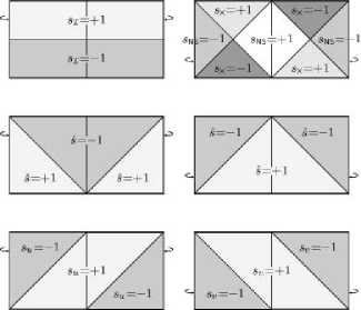
Figure 13: The values of the factors $s_{\scriptscriptstyle{\mathcal{I}}}$, $s_{\scriptscriptstyle\textsf{NS}}$, $s_{\!\times}$, $\check{s}$, $\hat{s}$, ${s_{u}}$ and ${s_{v}}$ in various regions of de Sitter space. The factors are defined in Eqs. (207), (195), (208), (155), (170) and (262), respectively. The factor $s_{\!\times}$ is used only in the expressions for static coordinates in the region where the Killing vector is spacelike. Therefore, we indicated the values of $s_{\!\times}$ only in those regions, although Eq. (208) defines $s_{\!\times}$ everywhere. The factors $s_{\!\times}$, ${s_{u}}$, and ${s_{v}}$ are defined only for any given section ${\vartheta=\text{constant}}$, but not as unique functions on the whole spacetime (they are not symmetric with respect to the pole). This is related to our convention using negative radial coordinates, cf. the text below Eq. (135).

A.1 The spherical cosmological family

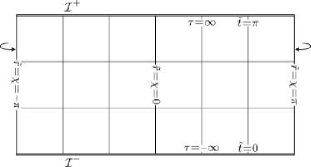
Figure 14: The spherical cosmological family of coordinates.

The first family consists of the standard or spherical cosmological coordinates ${\tau,\,\chi,\,\vartheta,\,\varphi}$, and of the standard rescaled or conformally Einstein coordinates ${{\tilde{t}},\,{\tilde{r}},\,\vartheta,\,\varphi}$ (where ${{\tilde{r}}\equiv\chi}$). These coordinates cover de Sitter spacetime globally. They are associated with cosmological observers with homogeneous spatial sections of positive spatial curvature. The coordinates are adjusted to the spherical symmetry of the spatial sections: ${\chi}$, ${\vartheta}$, and ${\varphi}$ are standard angular coordinates. The coordinate ${\tau}$ is a proper time along the worldlines of the cosmological observers given by ${\chi,\,\vartheta,\,\varphi=\text{constant}}$. The vector ${{{\partial}/{\partial\tau}}}$ is a conformal Killing vector which is everywhere timelike. The rescaled coordinates ${{\tilde{t}},\,{\tilde{r}},\,\vartheta,\,\varphi}$ can also be viewed as the standard coordinates of the conformally related Einstein universe; they cover smoothly both conformal infinities ${{\mathcal{I}}^{\pm}}$ of de Sitter spacetime.

Metric and relation between coordinates

$${\mathrm{\mathit{g}}}=-{\mathrm{\mathrm{d}}}\tau{}^{2}+\ell_{\scriptscriptstyle\Lambda}^{2}\,\cosh^{2}\!({\tau}/{\ell_{\scriptscriptstyle\Lambda}})\;\bigl{(}{\mathrm{\mathrm{d}}}\chi{}^{2}+\sin^{2}\!\chi\,{{\mathrm{\mathrm{d}\omega}}^{2}}\bigr{)}{\mbox{\;,}}$$ (140)

$${\mathrm{\mathit{g}}}=\ell_{\scriptscriptstyle\Lambda}^{2}\,\sin^{\!-2}\!{\tilde{t}}\;\bigl{(}-{\mathrm{\mathrm{d}}}{\tilde{t}}\,{}^{2}+{\mathrm{\mathrm{d}}}{\tilde{r}}{}^{2}+\sin^{2}\!{\tilde{r}}\,{{\mathrm{\mathrm{d}\omega}}^{2}}\bigr{)}{\mbox{\;,}}$$ (141)

$$\begin{gathered}\tan\frac{{\tilde{t}}}{2}=\exp\frac{\tau}{\ell_{\scriptscriptstyle\Lambda}}{\mbox{\;,\quad}}\cot{\tilde{t}}=-\sinh\frac{\tau}{\ell_{\scriptscriptstyle\Lambda}}{\mbox{\;,}}\\ \sin{\tilde{t}}=\cosh^{\!-1}\!\frac{\tau}{\ell_{\scriptscriptstyle\Lambda}}{\mbox{\;,\quad}}\cos{\tilde{t}}=-\tanh\frac{\tau}{\ell_{\scriptscriptstyle\Lambda}}{\mbox{\;,}}\end{gathered}$$ (142c)

$${\tilde{r}}=\chi{\mbox{\;.}}$$ (142d)

The ranges of coordinates are

$$\begin{gathered}\tau\in{\mathbb{R}}{\mbox{\;,\quad}}\chi\in(-\pi,\pi){\mbox{\;,}}\\ {\tilde{t}}\in(0,\pi){\mbox{\;,\quad}}{\tilde{r}}\in(-\pi,\pi){\mbox{\;,}}\end{gathered}$$ (143)

with negative values of radial coordinates $\chi$, ${\tilde{r}}$ interpreted in accordance with Eq. (136).

Orthonormal tetrad

$${{\mathrm{e}}_{\tau}} ={\frac{\partial}{\partial\tau}}=\frac{1}{\ell_{\scriptscriptstyle\Lambda}}\sin{\tilde{t}}\,{\frac{\partial}{\partial{\tilde{t}}}}{\mbox{\;,}}$$

$${{\mathrm{e}}_{\chi}} =\frac{1}{\ell_{\scriptscriptstyle\Lambda}}\cosh^{\!-1}\!\frac{\tau}{\ell_{\scriptscriptstyle\Lambda}}\,{\frac{\partial}{\partial\chi}}=\frac{1}{\ell_{\scriptscriptstyle\Lambda}}\sin{\tilde{t}}\,{\frac{\partial}{\partial{\tilde{r}}}}{\mbox{\;,}}$$ (144)

$${{\mathrm{e}}_{\vartheta}} =\frac{1}{\ell_{\scriptscriptstyle\Lambda}}\frac{1}{\cosh(\tau/\ell_{\scriptscriptstyle\Lambda})\sin\chi}{\frac{\partial}{\partial\vartheta}}=\frac{1}{\ell_{\scriptscriptstyle\Lambda}}\frac{\sin{\tilde{t}}}{\sin{\tilde{r}}}{\frac{\partial}{\partial\vartheta}}{\mbox{\;.}}$$

Relation to flat cosmological family

$$\tan{\tilde{t}} =\frac{2\,\ell_{\scriptscriptstyle\Lambda}{\hat{t}}}{\ell_{\scriptscriptstyle\Lambda}^{2}-{\hat{t}}^{2}+{\hat{r}}^{2}}=\frac{2\,\ell_{\scriptscriptstyle\Lambda}{\check{t}}}{\ell_{\scriptscriptstyle\Lambda}^{2}-{\check{t}}^{2}+{\check{r}}^{2}}{\mbox{\;,}}$$ (145)

$$\tan{\tilde{r}} =\frac{2\,\ell_{\scriptscriptstyle\Lambda}{\hat{r}}}{\ell_{\scriptscriptstyle\Lambda}^{2}+{\hat{t}}^{2}-{\hat{r}}^{2}}=\frac{2\,\ell_{\scriptscriptstyle\Lambda}{\check{r}}}{\ell_{\scriptscriptstyle\Lambda}^{2}+{\check{t}}^{2}-{\check{r}}^{2}}{\mbox{\;.}}$$

Relation to hyperbolic cosmological coordinates

$$\cot{\tilde{t}} =-\sinh\frac{\eta}{\ell_{\scriptscriptstyle\Lambda}}\,\cosh\frac{\rho}{\ell_{\scriptscriptstyle\Lambda}}{\mbox{\;,}}$$ (146)

$$\tan{\tilde{r}} ={\mspace{14.5mu}}\tanh\frac{\eta}{\ell_{\scriptscriptstyle\Lambda}}\,\sinh\frac{\rho}{\ell_{\scriptscriptstyle\Lambda}}{\mbox{\;.}}$$

Relation to static family in timelike domains N, S

$$\tan{\tilde{t}} =-s_{\scriptscriptstyle\textsf{NS}}\,\frac{\ell_{\scriptscriptstyle\Lambda}}{\sqrt{\ell_{\scriptscriptstyle\Lambda}^{2}-R^{2}}}\;{\sinh^{\!-1}\!\frac{T}{\ell_{\scriptscriptstyle\Lambda}}}{\mbox{\;,}}$$ (147)

$$\tan{\tilde{r}} =s_{\scriptscriptstyle\textsf{NS}}\,\frac{R}{\sqrt{\ell_{\scriptscriptstyle\Lambda}^{2}-R^{2}}}\;{\cosh^{\!-1}\!\frac{T}{\ell_{\scriptscriptstyle\Lambda}}}{\mbox{\;,}}$$

$$\tan{\tilde{t}}=-s_{\scriptscriptstyle\textsf{NS}}\,\frac{\cosh\frac{{\bar{r}}}{\ell_{\scriptscriptstyle\Lambda}}}{\sinh\frac{{\bar{t}}}{\ell_{\scriptscriptstyle\Lambda}}}{\mbox{\;,\quad}}\tan{\tilde{r}}=s_{\scriptscriptstyle\textsf{NS}}\,\frac{\sinh\frac{{\bar{r}}}{\ell_{\scriptscriptstyle\Lambda}}}{\cosh\frac{{\bar{t}}}{\ell_{\scriptscriptstyle\Lambda}}}{\mbox{\;,}}$$ (148)

where ${s_{\scriptscriptstyle\textsf{NS}}=+1}$ (${-1}$) in domain N (S), cf. Eq. (195).

Relation to static family in spacelike domains F, P

$$\tan{\tilde{t}} =\frac{-s_{\scriptscriptstyle{\mathcal{I}}}\,\ell_{\scriptscriptstyle\Lambda}}{\sqrt{R^{2}-\ell_{\scriptscriptstyle\Lambda}^{2}}}\;{\cosh^{\!-1}\!\frac{T}{\ell_{\scriptscriptstyle\Lambda}}}{\mbox{\;,}}$$ (149)

$$\tan{\tilde{r}} =\frac{s_{\scriptscriptstyle{\mathcal{I}}}\,R}{\sqrt{R^{2}-\ell_{\scriptscriptstyle\Lambda}^{2}}}\;{\sinh^{\!-1}\!\frac{T}{\ell_{\scriptscriptstyle\Lambda}}}{\mbox{\;,}}$$

$$\tan{\tilde{t}}=s_{\!\times}\,\frac{\sinh\frac{{\bar{r}}}{\ell_{\scriptscriptstyle\Lambda}}}{\cosh\frac{{\bar{t}}}{\ell_{\scriptscriptstyle\Lambda}}}{\mbox{\;,\quad}}\tan{\tilde{r}}=-s_{\!\times}\,\frac{\cosh\frac{{\bar{r}}}{\ell_{\scriptscriptstyle\Lambda}}}{\sinh\frac{{\bar{t}}}{\ell_{\scriptscriptstyle\Lambda}}}{\mbox{\;,}}$$ (150)

where ${s_{\scriptscriptstyle{\mathcal{I}}}=-\operatorname{sign}\cos{\tilde{t}}}$  and ${s_{\!\times}=-s_{\scriptscriptstyle{\mathcal{I}}}\,\operatorname{sign}{\tilde{r}}}$, cf. Eqs. (207) and (208).

Relation to conformally Minkowski coordinates

$$\cot{\tilde{t}}=\frac{2\ell_{\scriptscriptstyle\Lambda}t}{t^{2}-r^{2}-\ell_{\scriptscriptstyle\Lambda}^{2}}{\mbox{\;,\quad}}\tan{\tilde{r}}=\frac{2\ell_{\scriptscriptstyle\Lambda}r}{t^{2}-r^{2}+\ell_{\scriptscriptstyle\Lambda}^{2}}{\mbox{\;.}}$$ (151)

A.2 The flat cosmological family, type “$\vee$”

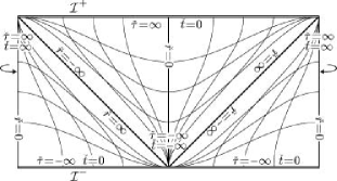
Figure 15: The flat cosmological family, type “$\vee$”.

The first flat cosmological coordinate family consists of the flat cosmological coordinates ${{\check{\tau}},\,{\check{r}},\,\vartheta,\,\varphi}$ and of the rescaled flat cosmological coordinates ${{\check{t}},\,{\check{r}},\,\vartheta,\,\varphi}$. Hypersurfaces ${{\check{\tau}}=\text{constant}}$ are homogeneous flat spaces and coordinate lines ${{\check{r}},\,\vartheta,\,\varphi=\text{constant}}$ are worldlines of cosmological observers orthogonal to these hypersurfaces. They are geodesic with proper time ${\check{\tau}}$, the vector ${{\partial}/{\partial{\check{\tau}}}}$ is a conformal Killing vector. The coordinates cover de Sitter spacetime smoothly, except for the past cosmological horizon, ${{\tilde{r}}={\tilde{t}}}$, of the north pole where ${{\check{r}},\,{\check{t}}\to\pm\infty}$. The coordinates thus split into two coordinate patches—“above” and “below” the horizon. The domain above the horizon has a cosmological interpretation of an exponentially expanding flat three-space. The rescaled coordinates can be viewed as inertial coordinates in the conformally related Minkowski space $\check{M}$, cf. Fig. 3; the domain above the horizon corresponds to the “lower half”, ${{\check{t}}<0}$, of $\check{M}$, the domain below corresponds to the “upper half”, ${{\check{t}}>0}$.

Metric and relation between coordinates

$${\mathrm{\mathit{g}}}=\frac{\ell_{\scriptscriptstyle\Lambda}^{2}}{{\check{t}}^{2}}\,\Bigl{(}-{\mathrm{\mathrm{d}}}{\check{t}}\,{}^{2}+{\mathrm{\mathrm{d}}}{\check{r}}{}^{2}+{\check{r}}^{2}\,{{\mathrm{\mathrm{d}\omega}}^{2}}\Bigr{)}{\mbox{\;,}}$$ (152)

$${\mathrm{\mathit{g}}}=-{\mathrm{\mathrm{d}}}{\check{\tau}}{}^{2}+\exp\bigl{(}{-\check{s}\,2\,{{\check{\tau}}}/{\ell_{\scriptscriptstyle\Lambda}}}\bigr{)}\,\bigl{(}{\mathrm{\mathrm{d}}}{\check{r}}{}^{2}+{\check{r}}^{2}\,{{\mathrm{\mathrm{d}\omega}}^{2}}\bigr{)}{\mbox{\;.}}$$ (153)

$${\check{t}}=\check{s}\,\ell_{\scriptscriptstyle\Lambda}\exp\Bigl{(}\check{s}\frac{{\check{\tau}}}{\ell_{\scriptscriptstyle\Lambda}}\Bigl{)}{\mbox{\;,}}$$ (154)

$$\check{s}=\operatorname{sign}{\check{t}}{\mbox{\;.}}$$ (155)

The ranges of coordinates are

$$\begin{gathered}{\check{\tau}}\in{\mathbb{R}}{\mbox{\;,\quad}}{\check{t}}\in{\mathbb{R}}^{-}{\mbox{\;,\quad}}{\check{r}}\in{\mathbb{R}}\quad\text{above the horizon}{\mbox{\;,}}\\ {\check{\tau}}\in{\mathbb{R}}{\mbox{\;,\quad}}{\check{t}}\in{\mathbb{R}}^{+}{\mbox{\;,\quad}}{\check{r}}\in{\mathbb{R}}\quad\text{below the horizon}{\mbox{\;,}}\end{gathered}$$ (156)

with negative values of radial coordinate ${\check{r}}$ interpreted as described in Eq. (136).

Orthonormal tetrad

$$\begin{gathered}{{\mathrm{e}}_{{\check{t}}}}={\frac{\partial}{\partial{\check{\tau}}}}=\frac{\check{s}\,{\check{t}}}{\ell_{\scriptscriptstyle\Lambda}}\,{\frac{\partial}{\partial{\check{t}}}}{\mbox{\;,\quad}}{{\mathrm{e}}_{{\check{r}}}}=\exp\frac{\check{s}{\check{\tau}}}{\ell_{\scriptscriptstyle\Lambda}}\,{\frac{\partial}{\partial{\check{r}}}}=\frac{\check{s}\,{\check{t}}}{\ell_{\scriptscriptstyle\Lambda}}\,{\frac{\partial}{\partial{\check{r}}}}{\mbox{\;,}}\\ {{\mathrm{e}}_{\vartheta}}=-\frac{\check{s}}{{\check{r}}}\exp\frac{\check{s}{\check{\tau}}}{\ell_{\scriptscriptstyle\Lambda}}\,{\frac{\partial}{\partial\vartheta}}=-\frac{1}{\ell_{\scriptscriptstyle\Lambda}}\frac{{\check{t}}}{{\check{r}}}\,{\frac{\partial}{\partial\vartheta}}{\mbox{\;.}}\end{gathered}$$ (157)

Relation to spherical cosmological family

$${\check{t}}=\frac{-\ell_{\scriptscriptstyle\Lambda}\cosh^{\!-1}\!(\tau/\ell_{\scriptscriptstyle\Lambda})}{\cos\chi+\tanh(\tau/\ell_{\scriptscriptstyle\Lambda})}{\mbox{\;,\quad}}{\check{r}}=\frac{\ell_{\scriptscriptstyle\Lambda}\cosh^{\!-1}\!(\tau/\ell_{\scriptscriptstyle\Lambda})}{\cos\chi+\tanh(\tau/\ell_{\scriptscriptstyle\Lambda})}{\mbox{\;.}}$$ (158)

$${\check{t}}=\frac{\ell_{\scriptscriptstyle\Lambda}\sin{\tilde{t}}}{\cos{\tilde{t}}-\cos{\tilde{r}}}{\mbox{\;,\quad}}{\check{r}}=\frac{\ell_{\scriptscriptstyle\Lambda}\sin{\tilde{r}}}{\cos{\tilde{r}}-\cos{\tilde{t}}}{\mbox{\;.}}$$ (159)

Relation to flat cosmological family, type “${\wedge}$”

$${\check{t}}=-\frac{{\hat{t}}\,\ell_{\scriptscriptstyle\Lambda}^{2}}{{\hat{t}}^{2}-{\hat{r}}^{2}}{\mbox{\;,\quad}}{\check{r}}=\frac{{\hat{r}}\,\ell_{\scriptscriptstyle\Lambda}^{2}}{{\hat{t}}^{2}-{\hat{r}}^{2}}{\mbox{\;,}}$$ (160)

$$\begin{gathered}{\check{t}}\,{\hat{r}}+{\hat{t}}\,{\check{r}}=0{\mbox{\;,\quad}}{\hat{t}}\,{\check{t}}+{\hat{r}}\,{\check{r}}=-\ell_{\scriptscriptstyle\Lambda}^{2}{\mbox{\;,}}\\ \bigl{(}-{\hat{t}}^{2}+{\hat{r}}^{2}\bigl{)}\bigl{(}-{\check{t}}^{2}+{\check{r}}^{2}\bigl{)}=\ell_{\scriptscriptstyle\Lambda}^{4}{\mbox{\;,}}\\ ({\hat{t}}+{\hat{r}})({\check{t}}+{\check{r}})=({\hat{t}}-{\hat{r}})({\check{t}}-{\check{r}})=-\ell_{\scriptscriptstyle\Lambda}^{2}{\mbox{\;.}}\end{gathered}$$ (161)

Relation to static family in timelike domains N, S

$$\begin{gathered}\frac{{\check{t}}}{\ell_{\scriptscriptstyle\Lambda}}=-s_{\scriptscriptstyle\textsf{NS}}\frac{\ell_{\scriptscriptstyle\Lambda}}{\sqrt{\ell_{\scriptscriptstyle\Lambda}^{2}-R^{2}}}\,\exp\Bigl{(}-\frac{T}{\ell_{\scriptscriptstyle\Lambda}}\Bigr{)}{\mbox{\;,}}\\ \frac{{\check{r}}}{\ell_{\scriptscriptstyle\Lambda}}={\mspace{14.5mu}}s_{\scriptscriptstyle\textsf{NS}}\frac{R}{\sqrt{\ell_{\scriptscriptstyle\Lambda}^{2}-R^{2}}}\,\exp\Bigl{(}-\frac{T}{\ell_{\scriptscriptstyle\Lambda}}\Bigr{)}{\mbox{\;,}}\end{gathered}$$ (162)

$$\begin{gathered}{\check{t}}=-s_{\scriptscriptstyle\textsf{NS}}\,\ell_{\scriptscriptstyle\Lambda}\exp\Bigl{(}-\frac{{\bar{t}}}{\ell_{\scriptscriptstyle\Lambda}}\Bigr{)}\,\cosh\frac{{\bar{r}}}{\ell_{\scriptscriptstyle\Lambda}}{\mbox{\;,}}\\ {\check{r}}={\mspace{14.5mu}}s_{\scriptscriptstyle\textsf{NS}}\ell_{\scriptscriptstyle\Lambda}\exp\Bigl{(}-\frac{{\bar{t}}}{\ell_{\scriptscriptstyle\Lambda}}\Bigr{)}\,\sinh\frac{{\bar{r}}}{\ell_{\scriptscriptstyle\Lambda}}{\mbox{\;,}}\end{gathered}$$ (163)

where ${s_{\scriptscriptstyle\textsf{NS}}=+1}$ (${-1}$) in domain N (S), cf. Eq. (195).

Relation to static family in spacelike domains F, P

$$\begin{gathered}\frac{{\check{t}}}{\ell_{\scriptscriptstyle\Lambda}}=s_{\!\times}\frac{\ell_{\scriptscriptstyle\Lambda}}{\sqrt{R^{2}-\ell_{\scriptscriptstyle\Lambda}^{2}}}\,\exp\Bigl{(}-\frac{T}{\ell_{\scriptscriptstyle\Lambda}}\Bigr{)}{\mbox{\;,}}\\ \frac{{\check{r}}}{\ell_{\scriptscriptstyle\Lambda}}=-s_{\!\times}\frac{R}{\sqrt{R^{2}-\ell_{\scriptscriptstyle\Lambda}^{2}}}\,\exp\Bigl{(}-\frac{T}{\ell_{\scriptscriptstyle\Lambda}}\Bigr{)}{\mbox{\;,}}\end{gathered}$$ (164)

$$\begin{gathered}{\check{t}}=s_{\!\times}\ell_{\scriptscriptstyle\Lambda}\exp\Bigl{(}-\frac{{\bar{t}}}{\ell_{\scriptscriptstyle\Lambda}}\Bigr{)}\,\sinh\frac{{\bar{r}}}{\ell_{\scriptscriptstyle\Lambda}}{\mbox{\;,}}\\ {\check{r}}=-s_{\!\times}\ell_{\scriptscriptstyle\Lambda}\exp\Bigl{(}-\frac{{\bar{t}}}{\ell_{\scriptscriptstyle\Lambda}}\Bigr{)}\,\cosh\frac{{\bar{r}}}{\ell_{\scriptscriptstyle\Lambda}}{\mbox{\;,}}\end{gathered}$$ (165)

where ${s_{\!\times}=\operatorname{sign}{\tilde{r}}\,\operatorname{sign}\cos{\tilde{t}}}$, cf. Eqs. (207) and (208).

Relation to conformally Minkowski coordinates

$$\frac{{\check{t}}}{\ell_{\scriptscriptstyle\Lambda}}=-\frac{\ell_{\scriptscriptstyle\Lambda}^{2}-t^{2}+r^{2}}{(\ell_{\scriptscriptstyle\Lambda}+t)^{2}-r^{2}}{\mbox{\;,\quad}}\frac{{\check{r}}}{\ell_{\scriptscriptstyle\Lambda}}=\frac{2\,\ell_{\scriptscriptstyle\Lambda}r}{(\ell_{\scriptscriptstyle\Lambda}+t)^{2}-r^{2}}{\mbox{\;.}}$$ (166)

A.3 The flat cosmological family, type “$\wedge$”

The second flat cosmological coordinate family consists of the flat cosmological coordinates ${{\hat{\tau}},\,{\hat{r}},\,\vartheta,\,\varphi}$ and of the rescaled flat cosmological coordinates ${{\hat{t}},\,{\hat{r}},\,\vartheta,\,\varphi}$. They can be built analogously to the flat coordinates introduced above, with north and south poles interchanged only. They thus have similar properties: Hypersurfaces ${{\hat{t}}=\text{constant}}$ are homogeneous flat three-spaces, coordinate lines ${{\hat{r}},\,\vartheta,\,\varphi=\text{constant}}$ are geodesics with proper time ${\hat{\tau}}$, and ${{\partial}/{\partial{\hat{\tau}}}}$ is a conformal Killing vector. The coordinates cover de Sitter spacetime everywhere except the future cosmological horizon, ${{\tilde{r}}=\pi-{\tilde{t}}}$, of the north pole (i.e., the past horizon of the south pole), and the rescaled coordinates can be viewed as inertial coordinates in the conformally related Minkowski space $\hat{M}$.

Metric and relation between coordinates

$${\mathrm{\mathit{g}}}=\frac{\ell_{\scriptscriptstyle\Lambda}^{2}}{{\hat{t}}^{2}}\,\Bigl{(}-{\mathrm{\mathrm{d}}}{\hat{t}}\,{}^{2}+{\mathrm{\mathrm{d}}}{\hat{r}}{}^{2}+{\hat{r}}^{2}\,{{\mathrm{\mathrm{d}\omega}}^{2}}\Bigr{)}{\mbox{\;,}}$$ (167)

$${\mathrm{\mathit{g}}}=-{\mathrm{\mathrm{d}}}{\hat{\tau}}{}^{2}+\exp\bigl{(}{-\hat{s}\,2\,{{\hat{\tau}}}/{\ell_{\scriptscriptstyle\Lambda}}}\bigr{)}\,\bigl{(}{\mathrm{\mathrm{d}}}{\hat{r}}{}^{2}+{\hat{r}}^{2}\,{{\mathrm{\mathrm{d}\omega}}^{2}}\bigr{)}{\mbox{\;,}}$$ (168)

$${\hat{t}}=\hat{s}\,\ell_{\scriptscriptstyle\Lambda}\exp\Bigl{(}\hat{s}\frac{{\hat{\tau}}}{\ell_{\scriptscriptstyle\Lambda}}\Bigl{)}{\mbox{\;,}}$$ (169)

where

$$\hat{s}=\operatorname{sign}{\hat{t}}{\mbox{\;.}}$$ (170)

The ranges of coordinates are

$$\begin{gathered}{\hat{\tau}}\in{\mathbb{R}}{\mbox{\;,\quad}}{\hat{t}}\in{\mathbb{R}}^{-}{\mbox{\;,\quad}}{\hat{r}}\in{\mathbb{R}}\quad\text{above the horizon}{\mbox{\;,}}\\ {\hat{\tau}}\in{\mathbb{R}}{\mbox{\;,\quad}}{\hat{t}}\in{\mathbb{R}}^{+}{\mbox{\;,\quad}}{\hat{r}}\in{\mathbb{R}}\quad\text{below the horizon}{\mbox{\;,}}\end{gathered}$$ (171)

with negative values of radial coordinate ${\hat{r}}$ interpreted as described in Eq. (136).

Orthonormal tetrad

$$\begin{gathered}{{\mathrm{e}}_{{\hat{t}}}}={\frac{\partial}{\partial{\hat{\tau}}}}=\frac{\hat{s}\,{\hat{t}}}{\ell_{\scriptscriptstyle\Lambda}}\,{\frac{\partial}{\partial{\hat{t}}}}{\mbox{\;,\quad}}{{\mathrm{e}}_{{\hat{r}}}}=\exp\frac{\hat{s}{\hat{\tau}}}{\ell_{\scriptscriptstyle\Lambda}}\,{\frac{\partial}{\partial{\hat{r}}}}=\frac{\hat{s}\,{\hat{t}}}{\ell_{\scriptscriptstyle\Lambda}}\,{\frac{\partial}{\partial{\hat{r}}}}{\mbox{\;,}}\\ {{\mathrm{e}}_{\vartheta}}=\frac{\hat{s}}{{\hat{r}}}\exp\frac{\hat{s}{\hat{\tau}}}{\ell_{\scriptscriptstyle\Lambda}}\,{\frac{\partial}{\partial\vartheta}}=\frac{1}{\ell_{\scriptscriptstyle\Lambda}}\frac{{\hat{t}}}{{\hat{r}}}\,{\frac{\partial}{\partial\vartheta}}{\mbox{\;.}}\end{gathered}$$ (172)

Relation to spherical cosmological family

$${\hat{t}}=\frac{\ell_{\scriptscriptstyle\Lambda}\cosh^{\!-1}\!(\tau/\ell_{\scriptscriptstyle\Lambda})}{\cos\chi-\tanh(\tau/\ell_{\scriptscriptstyle\Lambda})}{\mbox{\;,\quad}}{\hat{r}}=\frac{\ell_{\scriptscriptstyle\Lambda}\cosh^{\!-1}\!(\tau/\ell_{\scriptscriptstyle\Lambda})}{\cos\chi-\tanh(\tau/\ell_{\scriptscriptstyle\Lambda})}{\mbox{\;.}}$$ (173)

$${\hat{t}}=\frac{\ell_{\scriptscriptstyle\Lambda}\sin{\tilde{t}}}{\cos{\tilde{t}}+\cos{\tilde{r}}}{\mbox{\;,\quad}}{\hat{r}}=\frac{\ell_{\scriptscriptstyle\Lambda}\sin{\tilde{r}}}{\cos{\tilde{r}}+\cos{\tilde{t}}}{\mbox{\;.}}$$ (174)

Relation to flat cosmological family, type “${\wedge}$”

$${\hat{t}}=-\frac{{\check{t}}\,\ell_{\scriptscriptstyle\Lambda}^{2}}{{\check{t}}^{2}-{\check{r}}^{2}}{\mbox{\;,\quad}}{\hat{r}}=\frac{{\check{r}}\,\ell_{\scriptscriptstyle\Lambda}^{2}}{{\check{t}}^{2}-{\check{r}}^{2}}{\mbox{\;,}}$$ (175)

$$\begin{gathered}{\check{t}}\,{\hat{r}}+{\hat{t}}\,{\check{r}}=0{\mbox{\;,\quad}}{\hat{t}}\,{\check{t}}+{\hat{r}}\,{\check{r}}=-\ell_{\scriptscriptstyle\Lambda}^{2}{\mbox{\;,}}\\ \bigl{(}-{\hat{t}}^{2}+{\hat{r}}^{2}\bigl{)}\bigl{(}-{\check{t}}^{2}+{\check{r}}^{2}\bigl{)}=\ell_{\scriptscriptstyle\Lambda}^{4}{\mbox{\;,}}\\ ({\hat{t}}+{\hat{r}})({\check{t}}+{\check{r}})=({\hat{t}}-{\hat{r}})({\check{t}}-{\check{r}})=-\ell_{\scriptscriptstyle\Lambda}^{2}{\mbox{\;.}}\end{gathered}$$ (176)

Relation to static family in timelike domains N, S

$$\begin{gathered}\frac{{\hat{t}}}{\ell_{\scriptscriptstyle\Lambda}}=s_{\scriptscriptstyle\textsf{NS}}\,\frac{\ell_{\scriptscriptstyle\Lambda}}{\sqrt{\ell_{\scriptscriptstyle\Lambda}^{2}-R^{2}}}\,\exp\frac{T}{\ell_{\scriptscriptstyle\Lambda}}{\mbox{\;,}}\\ \frac{{\hat{r}}}{\ell_{\scriptscriptstyle\Lambda}}=s_{\scriptscriptstyle\textsf{NS}}\frac{R}{\sqrt{\ell_{\scriptscriptstyle\Lambda}^{2}-R^{2}}}\,\exp\frac{T}{\ell_{\scriptscriptstyle\Lambda}}{\mbox{\;,}}\end{gathered}$$ (177)

$$\begin{gathered}{\hat{t}}=s_{\scriptscriptstyle\textsf{NS}}\,\ell_{\scriptscriptstyle\Lambda}\exp\frac{{\bar{t}}}{\ell_{\scriptscriptstyle\Lambda}}\,\cosh\frac{{\bar{r}}}{\ell_{\scriptscriptstyle\Lambda}}{\mbox{\;,}}\\ {\hat{r}}=s_{\scriptscriptstyle\textsf{NS}}\,\ell_{\scriptscriptstyle\Lambda}\exp\frac{{\bar{t}}}{\ell_{\scriptscriptstyle\Lambda}}\,\sinh\frac{{\bar{r}}}{\ell_{\scriptscriptstyle\Lambda}}{\mbox{\;,}}\end{gathered}$$ (178)

where ${s_{\scriptscriptstyle\textsf{NS}}=+1}$ (${-1}$) in domain N (S), cf. Eq. (195).

Relation to static family in spacelike domains F, P

$$\begin{gathered}\frac{{\hat{t}}}{\ell_{\scriptscriptstyle\Lambda}}=s_{\!\times}\,\frac{\ell_{\scriptscriptstyle\Lambda}}{\sqrt{R^{2}-\ell_{\scriptscriptstyle\Lambda}^{2}}}\,\exp\frac{T}{\ell_{\scriptscriptstyle\Lambda}}{\mbox{\;,}}\\ \frac{{\hat{r}}}{\ell_{\scriptscriptstyle\Lambda}}=s_{\!\times}\,\frac{R}{\sqrt{R^{2}-\ell_{\scriptscriptstyle\Lambda}^{2}}}\,\exp\frac{T}{\ell_{\scriptscriptstyle\Lambda}}{\mbox{\;,}}\end{gathered}$$ (179)

$$\begin{gathered}{\hat{t}}=s_{\!\times}\,\ell_{\scriptscriptstyle\Lambda}\exp\frac{{\bar{t}}}{\ell_{\scriptscriptstyle\Lambda}}\,\sinh\frac{{\bar{r}}}{\ell_{\scriptscriptstyle\Lambda}}{\mbox{\;,}}\\ {\hat{r}}=s_{\!\times}\,\ell_{\scriptscriptstyle\Lambda}\exp\frac{{\bar{t}}}{\ell_{\scriptscriptstyle\Lambda}}\,\cosh\frac{{\bar{r}}}{\ell_{\scriptscriptstyle\Lambda}}{\mbox{\;,}}\end{gathered}$$ (180)

where ${s_{\!\times}=\operatorname{sign}{\tilde{r}}\,\operatorname{sign}\cos{\tilde{t}}}$, cf. Eqs. (207) and (208).

Relation to conformally Minkowski coordinates

$$\frac{{\hat{t}}}{\ell_{\scriptscriptstyle\Lambda}}=\frac{\ell_{\scriptscriptstyle\Lambda}^{2}-t^{2}+r^{2}}{(\ell_{\scriptscriptstyle\Lambda}-t)^{2}-r^{2}}{\mbox{\;,\quad}}\frac{{\hat{r}}}{\ell_{\scriptscriptstyle\Lambda}}=\frac{2\,\ell_{\scriptscriptstyle\Lambda}r}{(\ell_{\scriptscriptstyle\Lambda}-t)^{2}-r^{2}}{\mbox{\;.}}$$ (181)

A.4 The conformally Minkowski family

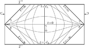
Figure 17: The conformally Minkowski family of coordinates.

The conformally Minkowski coordinates ${t,\,r,\,\vartheta,\,\varphi}$ can be understood as spherical coordinates in the conformally related Minkowski space ${M}$. The coordinates do not cover de Sitter spacetime globally—they cover only a region around north pole, see Fig. 17. The boundary of this region is given by the conformal infinity of the Minkowski spacetime. These coordinates are useful for studying the limit ${\Lambda\to 0}$.

The metric

$${\mathrm{\mathit{g}}}=\Bigl{(}\frac{2\,\ell_{\scriptscriptstyle\Lambda}^{2}}{\ell_{\scriptscriptstyle\Lambda}^{2}-t^{2}+r^{2}}\Bigr{)}^{2}\,\Bigl{(}-{\mathrm{\mathrm{d}}}t{}^{2}+{\mathrm{\mathrm{d}}}r{}^{2}+r^{2}\,{{\mathrm{\mathrm{d}\omega}}^{2}}\Bigr{)}{\mbox{\;,}}$$ (182)

the ranges of coordinates

$$t\in{\mathbb{R}}{\mbox{\;,\quad}}r\in{\mathbb{R}}{\mbox{\;,\quad}}\text{such that}\quad t^{2}-r^{2}<\ell_{\scriptscriptstyle\Lambda}^{2}{\mbox{\;,}}$$ (183)

with negative values of radial coordinate $r$ interpreted as described in Eq. (136).

Orthonormal tetrad

$$\begin{gathered}{{\mathrm{e}}_{t}}=\frac{\ell_{\scriptscriptstyle\Lambda}^{2}-t^{2}+r^{2}}{2\ell_{\scriptscriptstyle\Lambda}^{2}}\,{\frac{\partial}{\partial t}}{\mbox{\;,}}\\ {{\mathrm{e}}_{r}}=\frac{\ell_{\scriptscriptstyle\Lambda}^{2}-t^{2}+r^{2}}{2\ell_{\scriptscriptstyle\Lambda}^{2}}\,{\frac{\partial}{\partial r}}{\mbox{\;,}}\\ {{\mathrm{e}}_{\vartheta}}=\frac{\ell_{\scriptscriptstyle\Lambda}^{2}-t^{2}+r^{2}}{2\ell_{\scriptscriptstyle\Lambda}^{2}}\frac{1}{r}\,{\frac{\partial}{\partial t}}{\mbox{\;.}}\end{gathered}$$ (184)

Relation to spherical cosmological family

$$\begin{gathered}t=-\frac{\ell_{\scriptscriptstyle\Lambda}\cos{\tilde{t}}}{\cos{\tilde{r}}+\sin{\tilde{t}}}{\mbox{\;,}}\\ r={\mspace{14.5mu}}\frac{\ell_{\scriptscriptstyle\Lambda}\sin{\tilde{r}}}{\cos{\tilde{r}}+\sin{\tilde{t}}}{\mbox{\;.}}\end{gathered}$$ (185)

Relation to flat cosmological family

$$\frac{t}{\ell_{\scriptscriptstyle\Lambda}} =-\frac{\ell_{\scriptscriptstyle\Lambda}^{2}-{\hat{t}}^{2}+{\hat{r}}^{2}}{(\ell_{\scriptscriptstyle\Lambda}+{\hat{t}})^{2}-{\hat{r}}^{2}}=\frac{\ell_{\scriptscriptstyle\Lambda}^{2}-{\check{t}}^{2}+{\check{r}}^{2}}{(\ell_{\scriptscriptstyle\Lambda}-{\check{t}})^{2}-{\check{r}}^{2}}{\mbox{\;,}}$$ (186)

$$\frac{r}{\ell_{\scriptscriptstyle\Lambda}} ={\mspace{14.5mu}}\frac{2\,\ell_{\scriptscriptstyle\Lambda}{\hat{r}}}{(\ell_{\scriptscriptstyle\Lambda}+{\hat{t}})^{2}-{\hat{r}}^{2}}=\frac{2\,\ell_{\scriptscriptstyle\Lambda}{\check{r}}}{(\ell_{\scriptscriptstyle\Lambda}-{\check{t}})^{2}-{\check{r}}^{2}}{\mbox{\;.}}$$

Relation to hyperbolic cosmological coordinates

$$\frac{t}{\ell_{\scriptscriptstyle\Lambda}} =\tanh\frac{\eta}{2\ell_{\scriptscriptstyle\Lambda}}\,\cosh\frac{\beta}{\ell_{\scriptscriptstyle\Lambda}}{\mbox{\;,}}$$ (187)

$$\frac{r}{\ell_{\scriptscriptstyle\Lambda}} =\tanh\frac{\eta}{2\ell_{\scriptscriptstyle\Lambda}}\,\sinh\frac{\beta}{\ell_{\scriptscriptstyle\Lambda}}{\mbox{\;.}}$$

Relation to static family in timelike domains N, S

$$\frac{t}{\ell_{\scriptscriptstyle\Lambda}} =\frac{\sinh\frac{{\bar{t}}}{\ell_{\scriptscriptstyle\Lambda}}}{\cosh\frac{{\bar{t}}}{\ell_{\scriptscriptstyle\Lambda}}+s_{\scriptscriptstyle\textsf{NS}}\cosh\frac{{\bar{r}}}{\ell_{\scriptscriptstyle\Lambda}}}{\mbox{\;,}}$$ (188)

$$\frac{r}{\ell_{\scriptscriptstyle\Lambda}} =\frac{\sinh\frac{{\bar{r}}}{\ell_{\scriptscriptstyle\Lambda}}}{\cosh\frac{{\bar{r}}}{\ell_{\scriptscriptstyle\Lambda}}+s_{\scriptscriptstyle\textsf{NS}}\cosh\frac{{\bar{t}}}{\ell_{\scriptscriptstyle\Lambda}}}{\mbox{\;,}}$$

$$\frac{t}{\ell_{\scriptscriptstyle\Lambda}} =\frac{\sqrt{\ell_{\scriptscriptstyle\Lambda}^{2}-R^{2}}\,\sinh\frac{T}{\ell_{\scriptscriptstyle\Lambda}}}{s_{\scriptscriptstyle\textsf{NS}}\ell_{\scriptscriptstyle\Lambda}+\sqrt{\ell_{\scriptscriptstyle\Lambda}^{2}-R^{2}}\,\cosh\frac{T}{\ell_{\scriptscriptstyle\Lambda}}}{\mbox{\;,}}$$ (189)

$$\frac{r}{\ell_{\scriptscriptstyle\Lambda}} =\frac{R}{\ell_{\scriptscriptstyle\Lambda}+s_{\scriptscriptstyle\textsf{NS}}\sqrt{\ell_{\scriptscriptstyle\Lambda}^{2}-R^{2}}\,\cosh\frac{T}{\ell_{\scriptscriptstyle\Lambda}}}{\mbox{\;,}}$$

where ${s_{\scriptscriptstyle\textsf{NS}}=+1}$ (${-1}$) in domain N (S), cf. Eq. (195).

Relation to static family in spacelike domains F, P

$$\frac{t}{\ell_{\scriptscriptstyle\Lambda}} =\frac{\cosh\frac{{\bar{t}}}{\ell_{\scriptscriptstyle\Lambda}}}{\sinh\frac{{\bar{t}}}{\ell_{\scriptscriptstyle\Lambda}}-s_{\!\times}\sinh\frac{{\bar{r}}}{\ell_{\scriptscriptstyle\Lambda}}}{\mbox{\;,}}$$ (190)

$$\frac{r}{\ell_{\scriptscriptstyle\Lambda}} =\frac{\cosh\frac{{\bar{r}}}{\ell_{\scriptscriptstyle\Lambda}}}{\sinh\frac{{\bar{r}}}{\ell_{\scriptscriptstyle\Lambda}}-s_{\!\times}\cosh\frac{{\bar{t}}}{\ell_{\scriptscriptstyle\Lambda}}}{\mbox{\;,}}$$

$$\frac{t}{\ell_{\scriptscriptstyle\Lambda}} =\frac{\sqrt{R^{2}-\ell_{\scriptscriptstyle\Lambda}^{2}}\,\cosh\frac{T}{\ell_{\scriptscriptstyle\Lambda}}}{-s_{\!\times}\ell_{\scriptscriptstyle\Lambda}+\sqrt{R^{2}-\ell_{\scriptscriptstyle\Lambda}^{2}}\,\sinh\frac{T}{\ell_{\scriptscriptstyle\Lambda}}}{\mbox{\;,}}$$ (191)

$$\frac{r}{\ell_{\scriptscriptstyle\Lambda}} =\frac{R}{\ell_{\scriptscriptstyle\Lambda}-s_{\!\times}\sqrt{R^{2}-\ell_{\scriptscriptstyle\Lambda}^{2}}\,\sinh\frac{T}{\ell_{\scriptscriptstyle\Lambda}}}{\mbox{\;,}}$$

with ${s_{\!\times}=\operatorname{sign}{\tilde{r}}\,\operatorname{sign}\cos{\tilde{t}}}$, cf. Eqs. (207) and (208).

A.5 The static family in timelike domains N and S

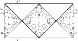
Figure 18: The static family of coordinates, timelike domains.

This family consists of the static coordinates $T$, $R$, $\vartheta$, $\varphi$ and the “tortoidal” static coordinates ${\bar{t}},\,{\bar{r}},\,\vartheta,\,\varphi$. The metric does not depend on time coordinate ${T={\bar{t}}}$—the coordinates are associated with a Killing vector. Since the Killing vector changes its character, the coordinates do not cover the spacetime smoothly. We first describe the static coordinates in domains N and S, where the Killing vector is timelike. In domain N the orbits of the Killing vector (corresponding to the worldlines of static observers) start and end at the north pole, in domain S—at the south pole. They are orthogonal to slices ${T=\text{constant}}$, each of which consists of two hemispheres (one in domain N, the other in S) with homogeneous spherical 3-metric. The distances between static observers (measured within these slices) do not change. Since the static observers must overcome first the cosmological contraction and then the expansion, they move with a (uniform) acceleration.

Metric and relation between coordinates

$${\mathrm{\mathit{g}}}=\cosh^{\!-2}\!\frac{{\bar{r}}}{\ell_{\scriptscriptstyle\Lambda}}\,\Bigl{(}-{\mathrm{\mathrm{d}}}{\bar{t}}{}^{2}+{\mathrm{\mathrm{d}}}{\bar{r}}{}^{2}+\ell_{\scriptscriptstyle\Lambda}^{2}\sinh^{2}\frac{{\bar{r}}}{\ell_{\scriptscriptstyle\Lambda}}\,{{\mathrm{\mathrm{d}\omega}}^{2}}\Bigr{)}{\mbox{\;,}}$$ (192)

$${\mathrm{\mathit{g}}}=\!-\Bigl{(}1-\frac{R^{2}}{\ell_{\scriptscriptstyle\Lambda}^{2}}\Bigr{)}\,{\mathrm{\mathrm{d}}}T{}^{2}+\Bigl{(}1-\frac{R^{2}}{\ell_{\scriptscriptstyle\Lambda}^{2}}\Bigr{)}^{\!\!-1}\!{\mathrm{\mathrm{d}}}R{}^{2}+R^{2}\,{{\mathrm{\mathrm{d}\omega}}^{2}}\!\!{\mbox{\;,}}\!\!$$ (193)

$$T={\bar{t}}{\mbox{\;,}}$$ (194a)

$$\exp\frac{{\bar{r}}}{\ell_{\scriptscriptstyle\Lambda}}=\sqrt{\frac{\ell_{\scriptscriptstyle\Lambda}+R}{\ell_{\scriptscriptstyle\Lambda}-R}}{\mbox{\;,}} \sinh\frac{{\bar{r}}}{\ell_{\scriptscriptstyle\Lambda}} =\frac{R}{\sqrt{\ell_{\scriptscriptstyle\Lambda}^{2}-R^{2}}}{\mbox{\;,}}$$ (194b)

$$\tanh\frac{{\bar{r}}}{\ell_{\scriptscriptstyle\Lambda}}=\frac{R}{\ell_{\scriptscriptstyle\Lambda}}{\mbox{\;,\quad}} \cosh\frac{{\bar{r}}}{\ell_{\scriptscriptstyle\Lambda}} =\frac{\ell_{\scriptscriptstyle\Lambda}}{\sqrt{\ell_{\scriptscriptstyle\Lambda}^{2}-R^{2}}}{\mbox{\;,}}$$

$$s_{\scriptscriptstyle\textsf{NS}}=\begin{cases}+1\quad\text{in domain ${{\textsf{N}}}$}{\mbox{\;,}}\\[2.15277pt] -1\quad\text{in domain ${{\textsf{S}}}$}{\mbox{\;.}}\end{cases}$$ (195)

The ranges of coordinates are

$$\begin{gathered}T\in{\mathbb{R}}{\mbox{\;,\quad}}R\in(-\ell_{\scriptscriptstyle\Lambda},\ell_{\scriptscriptstyle\Lambda}){\mbox{\;,}}\\ {\bar{t}}\in{\mathbb{R}}{\mbox{\;,\quad}}{\bar{r}}\in{\mathbb{R}}{\mbox{\;,}}\end{gathered}$$ (196)

with negative values of radial coordinate $R$ and ${\bar{r}}$ interpreted as described in Eq. (136).

Orthonormal tetrad

$$\begin{gathered}{{\mathrm{e}}_{T}}=\Bigl{(}1-\frac{R^{2}}{\ell_{\scriptscriptstyle\Lambda}^{2}}\Bigr{)}^{\!\!-1/2}{\frac{\partial}{\partial T}}=\cosh\frac{{\bar{r}}}{\ell_{\scriptscriptstyle\Lambda}}\,{\frac{\partial}{\partial{\bar{t}}}}{\mbox{\;,}}\\ {{\mathrm{e}}_{R}}=\Bigl{(}1-\frac{R^{2}}{\ell_{\scriptscriptstyle\Lambda}^{2}}\Bigr{)}^{1/2}{\frac{\partial}{\partial R}}=\cosh^{\!-1}\!\frac{{\bar{r}}}{\ell_{\scriptscriptstyle\Lambda}}\,{\frac{\partial}{\partial{\bar{r}}}}{\mbox{\;,}}\\ {{\mathrm{e}}_{\vartheta}}=\frac{1}{R}\,{\frac{\partial}{\partial\vartheta}}=\frac{1}{\ell_{\scriptscriptstyle\Lambda}}\coth\frac{{\bar{r}}}{\ell_{\scriptscriptstyle\Lambda}}\,{\frac{\partial}{\partial\vartheta}}{\mbox{\;.}}\end{gathered}$$ (197)

Relation to spherical cosmological family

$$T=\frac{\ell_{\scriptscriptstyle\Lambda}}{2}\,\log\frac{\cos{\tilde{r}}-\cos{\tilde{t}}}{\cos{\tilde{r}}+\cos{\tilde{t}}}{\mbox{\;,\quad}}R=\ell_{\scriptscriptstyle\Lambda}\,\frac{\sin{\tilde{r}}}{\sin{\tilde{t}}}{\mbox{\;,}}$$ (198)

$${\bar{t}}=\frac{\ell_{\scriptscriptstyle\Lambda}}{2}\,\log\Bigl{(}\tan{\frac{{\tilde{t}}+{\tilde{r}}}{2}}\;\tan{\frac{{\tilde{t}}-{\tilde{r}}}{2}}\Bigr{)}{\mbox{\;,}}$$ (199a)

$$\begin{aligned} &\exp\frac{{\bar{t}}}{\ell_{\scriptscriptstyle\Lambda}}=\sqrt{\frac{\cos{\tilde{r}}-\cos{\tilde{t}}}{\cos{\tilde{r}}+\cos{\tilde{t}}}}{\mbox{\;,}}\!\!&\sinh\frac{{\bar{t}}}{\ell_{\scriptscriptstyle\Lambda}}&=\frac{-s_{\scriptscriptstyle\textsf{NS}}\cos{\tilde{t}}}{\sqrt{\cos^{2}{\tilde{r}}-\cos^{2}{\tilde{t}}}}{\mbox{\;,}}\\ &\tanh\frac{{\bar{t}}}{\ell_{\scriptscriptstyle\Lambda}}=-\frac{\cos{\tilde{t}}}{\cos{\tilde{r}}}{\mbox{\;,}}&\cosh\frac{{\bar{t}}}{\ell_{\scriptscriptstyle\Lambda}}&=\frac{s_{\scriptscriptstyle\textsf{NS}}\cos{\tilde{r}}}{\sqrt{\cos^{2}{\tilde{r}}-\cos^{2}{\tilde{t}}}}{\mbox{\;,}}\end{aligned}$$

$${\bar{r}}=\frac{\ell_{\scriptscriptstyle\Lambda}}{2}\,\log\Bigl{(}\tan{\frac{{\tilde{t}}+{\tilde{r}}}{2}}\;\cot{\frac{{\tilde{t}}-{\tilde{r}}}{2}}\Bigr{)}{\mbox{\;,}}$$ (199b)

$$\begin{aligned} &\exp\frac{{\bar{r}}}{\ell_{\scriptscriptstyle\Lambda}}=\sqrt{\frac{\sin{\tilde{t}}+\sin{\tilde{r}}}{\sin{\tilde{t}}-\sin{\tilde{r}}}}{\mbox{\;,}}\!\!&\sinh\frac{{\bar{r}}}{\ell_{\scriptscriptstyle\Lambda}}&=\frac{\sin{\tilde{r}}}{\sqrt{\sin^{2}{\tilde{t}}-\sin^{2}{\tilde{r}}}}{\mbox{\;,}}\\ &\tanh\frac{{\bar{r}}}{\ell_{\scriptscriptstyle\Lambda}}=\frac{\sin{\tilde{r}}}{\sin{\tilde{t}}}{\mbox{\;,}}&\cosh\frac{{\bar{r}}}{\ell_{\scriptscriptstyle\Lambda}}&=\frac{\sin{\tilde{t}}}{\sqrt{\sin^{2}{\tilde{t}}-\sin^{2}{\tilde{r}}}}{\mbox{\;.}}\end{aligned}$$

Relation to flat cosmological family

$$\begin{gathered}{\bar{t}}=\frac{\ell_{\scriptscriptstyle\Lambda}}{2}\log\frac{{\hat{t}}^{2}-{\hat{r}}^{2}}{\ell_{\scriptscriptstyle\Lambda}^{2}}=-\frac{\ell_{\scriptscriptstyle\Lambda}}{2}\log\frac{{\check{t}}^{2}-{\check{r}}^{2}}{\ell_{\scriptscriptstyle\Lambda}^{2}}{\mbox{\;,}}\\ {\bar{r}}=\frac{\ell_{\scriptscriptstyle\Lambda}}{2}\log\frac{{\hat{t}}+{\hat{r}}}{{\hat{t}}-{\hat{r}}}=\frac{\ell_{\scriptscriptstyle\Lambda}}{2}\log\frac{{\check{t}}-{\check{r}}}{{\check{t}}+{\check{r}}}{\mbox{\;,}}\end{gathered}$$ (200)

$$\begin{gathered}\frac{T}{\ell_{\scriptscriptstyle\Lambda}}=\frac{1}{2}\log\frac{{\hat{t}}^{2}-{\hat{r}}^{2}}{\ell_{\scriptscriptstyle\Lambda}^{2}}=-\frac{1}{2}\log\frac{{\check{t}}^{2}-{\check{r}}^{2}}{\ell_{\scriptscriptstyle\Lambda}^{2}}{\mbox{\;,}}\\ \frac{R}{\ell_{\scriptscriptstyle\Lambda}}=\frac{{\hat{r}}}{{\hat{t}}}=-\frac{{\check{r}}}{{\check{t}}}{\mbox{\;.}}\end{gathered}$$ (201)

Relation to conformally Minkowski coordinates

$$\tanh\frac{T}{\ell_{\scriptscriptstyle\Lambda}}=\frac{2\,\ell_{\scriptscriptstyle\Lambda}t}{\ell_{\scriptscriptstyle\Lambda}^{2}+t^{2}-r^{2}}{\mbox{\;,\quad}}\frac{R}{\ell_{\scriptscriptstyle\Lambda}}=\frac{2\,\ell_{\scriptscriptstyle\Lambda}r}{\ell_{\scriptscriptstyle\Lambda}^{2}+r^{2}-t^{2}}{\mbox{\;,}}$$ (202)

$${\bar{t}}=\frac{\ell_{\scriptscriptstyle\Lambda}}{2}\log\frac{(\ell_{\scriptscriptstyle\Lambda}+t)^{2}-r^{2}}{(\ell_{\scriptscriptstyle\Lambda}-t)^{2}-r^{2}}{\mbox{\;,\quad}}{\bar{r}}=\frac{\ell_{\scriptscriptstyle\Lambda}}{2}\log\frac{(\ell_{\scriptscriptstyle\Lambda}+r)^{2}-t^{2}}{(\ell_{\scriptscriptstyle\Lambda}-r)^{2}-t^{2}}{\mbox{\;.}}$$ (203)

A.6 The static family in spacelike domains F and P

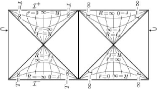
Figure 19: ​The static family of coordinates, spacelike domains.

Here we describe the static coordinates ${T,\,R,\,\vartheta,\,\varphi}$ and the “tortoidal” static coordinates ${{\bar{t}},\,{\bar{r}},\,\vartheta,\,\varphi}$ from the preceding section in domains F and S where the Killing vector is spacelike. These “non-static” domains extend up to infinity, namely, domain F up to ${{\mathcal{I}}^{+}}$, domain P up to ${{\mathcal{I}}^{-}}$. The orbits of the Killing vector start at the south pole and end at the north pole in F, and they point in opposite direction in P. The motion along them could thus be characterized as a “translation” from one pole to the other. The Lorentzian hypersurfaces ${T=\text{constant}}$ are homogeneous spaces with positive curvature, i.e., 3-dimensional de Sitter spacetimes.

Metric and relation between coordinates

$${\mathrm{\mathit{g}}}=\sinh^{\!-2}\!\frac{{\bar{r}}}{\ell_{\scriptscriptstyle\Lambda}}\,\Bigl{(}-{\mathrm{\mathrm{d}}}{\bar{r}}{}^{2}+{\mathrm{\mathrm{d}}}{\bar{t}}{}^{2}+\ell_{\scriptscriptstyle\Lambda}^{2}\cosh^{2}\frac{{\bar{r}}}{\ell_{\scriptscriptstyle\Lambda}}\,{{\mathrm{\mathrm{d}\omega}}^{2}}\Bigr{)}{\mbox{\;,}}$$ (204)

$${\mathrm{\mathit{g}}}=\!-\Bigl{(}1-\frac{R^{2}}{\ell_{\scriptscriptstyle\Lambda}^{2}}\Bigr{)}\,{\mathrm{\mathrm{d}}}T{}^{2}+\!\Bigl{(}1-\frac{R^{2}}{\ell_{\scriptscriptstyle\Lambda}^{2}}\Bigr{)}^{\!\!-1}\!{\mathrm{\mathrm{d}}}R{}^{2}+R^{2}\,{{\mathrm{\mathrm{d}\omega}}^{2}}\!\!{\mbox{\;,}}\!\!$$ (205)

$$T={\bar{t}}{\mbox{\;,}}$$ (206a)

$$\exp\frac{{\bar{r}}}{\ell_{\scriptscriptstyle\Lambda}}=\sqrt{\frac{R+\ell_{\scriptscriptstyle\Lambda}}{R-\ell_{\scriptscriptstyle\Lambda}}}{\mbox{\;,}}\!\! \left\lvert\sinh\frac{{\bar{r}}}{\ell_{\scriptscriptstyle\Lambda}}\right\rvert=\frac{\ell_{\scriptscriptstyle\Lambda}}{\sqrt{R^{2}-\ell_{\scriptscriptstyle\Lambda}^{2}}}{\mbox{\;,}}$$ (206b)

$$\tanh\frac{{\bar{r}}}{\ell_{\scriptscriptstyle\Lambda}}=\frac{\ell_{\scriptscriptstyle\Lambda}}{R}{\mbox{\;,}}\!\! \cosh\frac{{\bar{r}}}{\ell_{\scriptscriptstyle\Lambda}}=\frac{\left\lvert R\right\rvert}{\sqrt{R^{2}-\ell_{\scriptscriptstyle\Lambda}^{2}}}{\mbox{\;.}}$$

The signature factors $s_{\scriptscriptstyle{\mathcal{I}}}$ and $s_{\!\times}$ are defined as

$$s_{\scriptscriptstyle{\mathcal{I}}}=\begin{cases}+1\quad\text{in domain ${{\textsf{F}}}$}{\mbox{\;,}}\\[2.15277pt] -1\quad\text{in domain ${{\textsf{P}}}$}{\mbox{\;,}}\end{cases}$$ (207)

and

$$s_{\!\times}=-s_{\scriptscriptstyle{\mathcal{I}}}\,\operatorname{sign}{\tilde{r}}{\mbox{\;.}}$$ (208)

The coordinates ranges are

$$\begin{gathered}T\in{\mathbb{R}}{\mbox{\;,\quad}}\left\lvert R\right\rvert\in(\ell_{\scriptscriptstyle\Lambda},\infty){\mbox{\;,}}\\ {\bar{t}}\in{\mathbb{R}}{\mbox{\;,\quad}}{\bar{r}}\in{\mathbb{R}}{\mbox{\;,}}\end{gathered}$$ (209)

with negative values of radial coordinate $R$ and ${\bar{r}}$ interpreted as described in Eq. (136).

Orthonormal tetrad

$$\begin{gathered}{{\mathrm{e}}_{T}}=\Bigl{(}\frac{R^{2}}{\ell_{\scriptscriptstyle\Lambda}^{2}}-1\Bigr{)}^{\!\!-1/2}{\frac{\partial}{\partial T}}=\left\lvert\,\sinh\frac{{\bar{r}}}{\ell_{\scriptscriptstyle\Lambda}}\right\rvert\,{\frac{\partial}{\partial{\bar{t}}}}{\mbox{\;,}}\\ {{\mathrm{e}}_{R}}=\Bigl{(}\frac{R^{2}}{\ell_{\scriptscriptstyle\Lambda}^{2}}-1\Bigr{)}^{1/2}{\frac{\partial}{\partial R}}=-\!\left\lvert\,\sinh^{\!-1}\!\frac{{\bar{r}}}{\ell_{\scriptscriptstyle\Lambda}}\right\rvert\,{\frac{\partial}{\partial{\bar{r}}}}{\mbox{\;,}}\\ {{\mathrm{e}}_{\vartheta}}=\frac{1}{R}\,{\frac{\partial}{\partial\vartheta}}=\frac{1}{\ell_{\scriptscriptstyle\Lambda}}\left\lvert\,\tanh\frac{{\bar{r}}}{\ell_{\scriptscriptstyle\Lambda}}\right\rvert\,{\frac{\partial}{\partial\vartheta}}{\mbox{\;.}}\end{gathered}$$ (210)

Relation to spherical cosmological family

$$T=\frac{\ell_{\scriptscriptstyle\Lambda}}{2}\,\log\frac{\cos{\tilde{t}}-\cos{\tilde{r}}}{\cos{\tilde{t}}+\cos{\tilde{r}}}{\mbox{\;,\quad}}R=\ell_{\scriptscriptstyle\Lambda}\,\frac{\sin{\tilde{r}}}{\sin{\tilde{t}}}{\mbox{\;,}}$$ (211)

$${\bar{t}}=\frac{\ell_{\scriptscriptstyle\Lambda}}{2}\,\log\Bigl{(}-\tan{\frac{{\tilde{t}}+{\tilde{r}}}{2}}\;\tan{\frac{{\tilde{t}}-{\tilde{r}}}{2}}\Bigr{)}{\mbox{\;,}}$$ (212a)

$$\begin{aligned} &\exp\frac{{\bar{t}}}{\ell_{\scriptscriptstyle\Lambda}}=\sqrt{\frac{\cos{\tilde{t}}-\cos{\tilde{r}}}{\cos{\tilde{t}}+\cos{\tilde{r}}}}{\mbox{\;,}}\!\!&\sinh\frac{{\bar{t}}}{\ell_{\scriptscriptstyle\Lambda}}&=\frac{s_{\scriptscriptstyle{\mathcal{I}}}\cos{\tilde{r}}}{\sqrt{\cos^{2}{\tilde{t}}-\cos^{2}{\tilde{r}}}}{\mbox{\;,}}\\ &\tanh\frac{{\bar{t}}}{\ell_{\scriptscriptstyle\Lambda}}=-\frac{\cos{\tilde{r}}}{\cos{\tilde{t}}}{\mbox{\;,}}&\cosh\frac{{\bar{t}}}{\ell_{\scriptscriptstyle\Lambda}}&=\frac{-s_{\scriptscriptstyle{\mathcal{I}}}\cos{\tilde{t}}}{\sqrt{\cos^{2}{\tilde{t}}-\cos^{2}{\tilde{r}}}}{\mbox{\;,}}\end{aligned}$$

$${\bar{r}}=\frac{\ell_{\scriptscriptstyle\Lambda}}{2}\,\log\Bigl{(}-\tan{\frac{{\tilde{t}}+{\tilde{r}}}{2}}\;\cot{\frac{{\tilde{t}}-{\tilde{r}}}{2}}\Bigr{)}{\mbox{\;,}}$$ (212b)

$$\begin{aligned} &\exp\frac{{\bar{r}}}{\ell_{\scriptscriptstyle\Lambda}}=\sqrt{\frac{\sin{\tilde{r}}+\sin{\tilde{t}}}{\sin{\tilde{r}}-\sin{\tilde{t}}}}{\mbox{\;,}}\!\!&\left\lvert\sinh\frac{{\bar{r}}}{\ell_{\scriptscriptstyle\Lambda}}\right\rvert&=\frac{\sin{\tilde{t}}}{\sqrt{\sin^{2}{\tilde{r}}-\sin^{2}{\tilde{t}}}}{\mbox{\;,}}\\ &\tanh\frac{{\bar{r}}}{\ell_{\scriptscriptstyle\Lambda}}={\mspace{14.5mu}}\frac{\sin{\tilde{t}}}{\sin{\tilde{r}}}{\mbox{\;,}}&\cosh\frac{{\bar{r}}}{\ell_{\scriptscriptstyle\Lambda}}&=\frac{\left\lvert\sin{\tilde{r}}\right\rvert}{\sqrt{\sin^{2}{\tilde{r}}-\sin^{2}{\tilde{t}}}}{\mbox{\;.}}\end{aligned}$$

Relation to flat cosmological family

$$\begin{gathered}{\bar{t}}=\frac{\ell_{\scriptscriptstyle\Lambda}}{2}\log\frac{-{\hat{t}}^{2}+{\hat{r}}^{2}}{\ell_{\scriptscriptstyle\Lambda}^{2}}=-\frac{\ell_{\scriptscriptstyle\Lambda}}{2}\log\frac{-{\check{t}}^{2}+{\check{r}}^{2}}{\ell_{\scriptscriptstyle\Lambda}^{2}}{\mbox{\;,}}\\ {\bar{r}}=\frac{\ell_{\scriptscriptstyle\Lambda}}{2}\log\frac{{\hat{r}}+{\hat{t}}}{{\hat{r}}-{\hat{t}}}=\frac{\ell_{\scriptscriptstyle\Lambda}}{2}\log\frac{{\check{r}}-{\check{t}}}{{\check{r}}+{\check{t}}}{\mbox{\;,}}\end{gathered}$$ (213)

$$\begin{gathered}\frac{T}{\ell_{\scriptscriptstyle\Lambda}}=\frac{1}{2}\log\frac{-{\hat{t}}^{2}+{\hat{r}}^{2}}{\ell_{\scriptscriptstyle\Lambda}^{2}}=-\frac{1}{2}\log\frac{-{\check{t}}^{2}+{\check{r}}^{2}}{\ell_{\scriptscriptstyle\Lambda}^{2}}{\mbox{\;,}}\\ \frac{R}{\ell_{\scriptscriptstyle\Lambda}}=\frac{{\hat{r}}}{{\hat{t}}}=-\frac{{\check{r}}}{{\check{t}}}{\mbox{\;.}}\end{gathered}$$ (214)

Relation to conformally Minkowski coordinates

$$\coth\frac{T}{\ell_{\scriptscriptstyle\Lambda}}=\frac{2\,\ell_{\scriptscriptstyle\Lambda}t}{\ell_{\scriptscriptstyle\Lambda}^{2}+t^{2}-r^{2}}{\mbox{\;,\quad}}\frac{R}{\ell_{\scriptscriptstyle\Lambda}}=\frac{2\,\ell_{\scriptscriptstyle\Lambda}r}{\ell_{\scriptscriptstyle\Lambda}^{2}+r^{2}-t^{2}}{\mbox{\;,}}$$ (215)

$$\begin{gathered}{\bar{t}}=\frac{\ell_{\scriptscriptstyle\Lambda}}{2}\log\Bigl{(}-\frac{(\ell_{\scriptscriptstyle\Lambda}+t)^{2}-r^{2}}{(\ell_{\scriptscriptstyle\Lambda}-t)^{2}-r^{2}}\Bigr{)}{\mbox{\;,}}\\ {\bar{r}}=\frac{\ell_{\scriptscriptstyle\Lambda}}{2}\log\Bigl{(}-\frac{(\ell_{\scriptscriptstyle\Lambda}+r)^{2}-t^{2}}{(\ell_{\scriptscriptstyle\Lambda}-r)^{2}-t^{2}}\Bigr{)}{\mbox{\;,}}\end{gathered}$$ (216)

A.7 The hyperbolic cosmological family

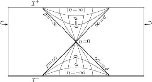
Figure 20: The hyperbolic cosmological family of coordinates.

The third type of cosmological coordinates are the hyperbolic cosmological coordinates ${\eta,\,\rho,\,\vartheta,\varphi}$. The hypersurfaces ${\eta=\text{constant}}$ are homogeneous spaces with negative curvature, coordinate lines ${\rho,\vartheta,\varphi=\text{constant}}$ correspond to the worldlines of cosmological observers orthogonal to these slices, and the vector ${{{\partial}/{\partial\eta}}}$ is a timelike conformal Killing vector. The coordinates cover spacetime only partially—they can be introduced in two disconnected domains near the north pole, namely, in the past of the event ${{\tilde{t}}=\pi/2}$, ${{\tilde{r}}=0}$ (where ${\eta<0}$), and in the future of this event (where ${\eta>0}$).

The metric

$${\mathrm{\mathit{g}}}=-{\mathrm{\mathrm{d}}}\eta{}^{2}+{\textstyle\sinh^{2}\!\frac{\eta}{\ell_{\scriptscriptstyle\Lambda}}}\,\bigl{(}{\mathrm{\mathrm{d}}}\rho{}^{2}+\ell_{\scriptscriptstyle\Lambda}^{2}{\textstyle\sinh^{2}\!\frac{\rho}{\ell_{\scriptscriptstyle\Lambda}}}\,{{\mathrm{\mathrm{d}\omega}}^{2}}\bigr{)}{\mbox{\;,}}$$ (217)

The ranges of coordinates and the signature factor $s_{\scriptscriptstyle{\mathcal{I}}}$ are

$$\eta\in{\mathbb{R}}^{+}{\mbox{\;,\quad}}\rho\in{\mathbb{R}}{\mbox{\;,\quad}}s_{\scriptscriptstyle{\mathcal{I}}}=+1$$ in the future patch , (218)

$$\eta\in{\mathbb{R}}^{-}{\mbox{\;,\quad}}\rho\in{\mathbb{R}}{\mbox{\;,\quad}}s_{\scriptscriptstyle{\mathcal{I}}}=-1$$ in the past patch ,

with negative values of radial coordinate $\rho$ interpreted as described in Eq. (136).

Orthonormal tetrad

$$\begin{gathered}{{\mathrm{e}}_{\eta}}={\frac{\partial}{\partial\eta}}{\mbox{\;,\quad}}{{\mathrm{e}}_{\rho}}=\sinh^{\!-1}\!\frac{\eta}{\ell_{\scriptscriptstyle\Lambda}}\;{\frac{\partial}{\partial\rho}}{\mbox{\;,}}\\ {{\mathrm{e}}_{\vartheta}}=\sinh^{\!-1}\!\frac{\eta}{\ell_{\scriptscriptstyle\Lambda}}\,\sinh^{\!-1}\!\frac{\rho}{\ell_{\scriptscriptstyle\Lambda}}\;{\frac{\partial}{\partial\rho}}{\mbox{\;.}}\end{gathered}$$ (219)

Relation to spherical cosmological family

$$\tanh\frac{\eta}{2\ell_{\scriptscriptstyle\Lambda}}=s_{\scriptscriptstyle{\mathcal{I}}}\sqrt{\frac{\cos{\tilde{r}}-\sin{\tilde{t}}}{\cos{\tilde{r}}+\sin{\tilde{t}}}}{\mbox{\;,\quad}}\tanh\frac{\rho}{\ell_{\scriptscriptstyle\Lambda}}=-\frac{\sin{\tilde{r}}}{\cos{\tilde{t}}}{\mbox{\;.}}$$ (220)

Relation to conformally Minkowski coordinates

$$\tanh\frac{\eta}{2\ell_{\scriptscriptstyle\Lambda}}=s_{\scriptscriptstyle{\mathcal{I}}}{\frac{\sqrt{t^{2}-r^{2}}}{\ell_{\scriptscriptstyle\Lambda}}}{\mbox{\;,\quad}}\tanh\frac{\rho}{\ell_{\scriptscriptstyle\Lambda}}=\frac{r}{t}{\mbox{\;.}}$$ (221)

A.8 The accelerated coordinate family

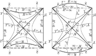
Figure 21: The accelerated family of coordinates.

This family consists of the accelerated coordinates ${{T^{\prime}}{},\,{R^{\prime}}{},\,{\vartheta^{\prime}},\,\varphi}$, and the C-metric-like coordinates ${\tau,\,\upsilon,\,\xi,\,\varphi}$ ($\tau$ being different from ${\tau}$ of the standard coordinates). Contrary to the previous cases the accelerated coordinates are centered on uniformly accelerate origins: ${{R^{\prime}}{}=0}$ corresponds to two worldlines with acceleration ${\left\lvert a_{\mathrm{o}}\right\rvert}$. The transformation relations to the systems introduced above mix these three coordinates in general.

The accelerated coordinates are closely related to the static system. Their time coordinates coincide, ${{T^{\prime}}{}\!=\!T}$, and coordinate lines ${{R^{\prime}}{},{\vartheta^{\prime}},\varphi=\text{constant}}$ are the same as those with ${R,\vartheta,\varphi=\text{constant}}$. Both coordinate systems are identical for ${a_{\mathrm{o}}=0}$. Sections ${T,{T^{\prime}}{},\varphi\!=\!\text{constant}}$ with ${R,{R^{\prime}}{}<\ell_{\scriptscriptstyle\Lambda}}$ have geometry of 2-sphere with parallels and meridians given by the coordinate lines of the static coordinates ${R,\,\vartheta}$. The lines of coordinates ${{R^{\prime}}{},\,{\vartheta^{\prime}}}$ are the deformed version of static ones, their poles are shifted along meridian ${\vartheta=0}$ towards each other, cf. Fig. 11.

Two conformal diagrams of sections ${{\vartheta^{\prime}},\varphi=\text{constant}}$ (${{\vartheta^{\prime}}<\pi/2}$ on the right, ${{\vartheta^{\prime}}>\pi/2}$ on the left), adapted to the accelerated coordinates, are depicted in Fig. 21. The shape of the diagram varies with different values of ${{\vartheta^{\prime}}}$; indeed, the position of infinity is given by ${R^{\prime}}{}={-\ell_{\scriptscriptstyle\Lambda}^{2}/R_{\mathrm{o}}\,\cos^{\!-1}{\vartheta^{\prime}}}$. See also Fig. 10 for sections ${{\vartheta^{\prime}}=0,\pi}$.

The C-metric-like coordinates rescale only the values of the accelerated coordinates and regularize the coordinate singularity ${{R^{\prime}}{}=\pm\infty}$. de Sitter metric in these coordinates is a zero-mass limit of the C-metric (the metric describing accelerated black holes; see, e.g., Podolský et al. (2003); Dias and Lemos (2003a)).

Finally, we use four parameters ${a_{\mathrm{o}},\,\alpha_{\mathrm{o}},\,R_{\mathrm{o}},\,b_{\mathrm{o}}}$ to parametrize the acceleration.They are related as follows:

$$\sinh\alpha_{\mathrm{o}} \;=\; \frac{R_{\mathrm{o}}}{\sqrt{\ell_{\scriptscriptstyle\Lambda}^{2}-R_{\mathrm{o}}^{2}}} \;=\; \frac{b_{\mathrm{o}}^{2}-\ell_{\scriptscriptstyle\Lambda}^{2}}{2\,\ell_{\scriptscriptstyle\Lambda}b_{\mathrm{o}}} \;=\; \quad\!-a_{\mathrm{o}}\ell_{\scriptscriptstyle\Lambda}{\mbox{\;,}}$$

$$\cosh\alpha_{\mathrm{o}} \;=\; \frac{\ell_{\scriptscriptstyle\Lambda}}{\sqrt{\ell_{\scriptscriptstyle\Lambda}^{2}-R_{\mathrm{o}}^{2}}} \;=\; \frac{b_{\mathrm{o}}^{2}+\ell_{\scriptscriptstyle\Lambda}^{2}}{2\,\ell_{\scriptscriptstyle\Lambda}b_{\mathrm{o}}} \;=\; \sqrt{1+a_{\mathrm{o}}^{2}\ell_{\scriptscriptstyle\Lambda}^{2}}{\mbox{\;,}}$$

$$\tanh\alpha_{\mathrm{o}} \;=\; \qquad\!\frac{R_{\mathrm{o}}}{\ell_{\scriptscriptstyle\Lambda}} \;=\; \frac{b_{\mathrm{o}}^{2}-\ell_{\scriptscriptstyle\Lambda}^{2}}{b_{\mathrm{o}}^{2}+\ell_{\scriptscriptstyle\Lambda}^{2}} \;=\; -\frac{a_{\mathrm{o}}\ell_{\scriptscriptstyle\Lambda}}{\sqrt{1+a_{\mathrm{o}}^{2}\ell_{\scriptscriptstyle\Lambda}^{2}}}{\mbox{\;,}}$$

$$\exp\alpha_{\mathrm{o}} \;=\; \sqrt{\frac{\ell_{\scriptscriptstyle\Lambda}+R_{\mathrm{o}}}{\ell_{\scriptscriptstyle\Lambda}-R_{\mathrm{o}}}} \;=\; \quad\,\frac{b_{\mathrm{o}}}{\ell_{\scriptscriptstyle\Lambda}} \;=\; \sqrt{1+a_{\mathrm{o}}^{2}\ell_{\scriptscriptstyle\Lambda}^{2}}-a_{\mathrm{o}}\ell_{\scriptscriptstyle\Lambda}{\mbox{\;.}}$$

Metric and relation between coordinates

$${\mathrm{\mathit{g}}}\!=\!\Omega^{2}\biggl{[}-\Bigl{(}1\!-\!\frac{{R^{\prime}}{}^{2}}{\ell_{\scriptscriptstyle\Lambda}^{2}}\Bigr{)}\,{\mathrm{\mathrm{d}}}{T^{\prime}}{}{}^{2}+\!\Bigl{(}1\!-\!\frac{{R^{\prime}}{}^{2}}{\ell_{\scriptscriptstyle\Lambda}^{2}}\Bigr{)}^{\!\!-1}{\mathrm{\mathrm{d}}}{R^{\prime}}{}{}^{2}+{R^{\prime}}{}^{2}\,{{\mathrm{\mathrm{d}\omega}}^{2}}{}^{\prime}\biggr{]}\!\!{\mbox{\;,}}$$ (223)

$${\mathrm{\mathit{g}}}\!=\!{\mathfrak{r}}^{2}\mspace{-1.0mu}\biggl{[}-(\upsilon^{2}\!{-}1)\,{\mathrm{\mathrm{d}}}\tau{}^{2}{+}\frac{1}{\upsilon^{2}\!{-}1}\,{\mathrm{\mathrm{d}}}\upsilon{}^{2}{+}\frac{1}{1{-}\xi^{2}}\,{\mathrm{\mathrm{d}}}\xi{}^{2}{+}(1{-}\xi^{2})\,{\mathrm{\mathrm{d}}}\varphi{}^{2}\biggr{]}\!\!{\mbox{\;,}}$$ (224)

where

$${{\mathrm{\mathrm{d}\omega}}^{2}}{}^{\prime}=\bigl{(}{\mathrm{\mathrm{d}}}{\vartheta^{\prime}}{}^{2}+\sin^{2}{\vartheta^{\prime}}\,{\mathrm{\mathrm{d}}}\varphi{}^{2}\bigr{)}{\mbox{\;,}}$$ (225)

$$\Omega=\frac{\sqrt{1-{R_{\mathrm{o}}^{2}}/{\ell_{\scriptscriptstyle\Lambda}^{2}}}}{1+({{R^{\prime}}{}R_{\mathrm{o}}}/{\ell_{\scriptscriptstyle\Lambda}^{2}})\cos{\vartheta^{\prime}}}=\frac{{\mathfrak{r}}}{{R^{\prime}}{}}=\frac{{\mathfrak{r}}\,\upsilon}{\ell_{\scriptscriptstyle\Lambda}}{\mbox{\;,}}$$ (226)

$${\mathfrak{r}}=\frac{\ell_{\scriptscriptstyle\Lambda}}{\upsilon\cosh\alpha_{\mathrm{o}}-\xi\sinh\alpha_{\mathrm{o}}}=\Omega\,{R^{\prime}}{}=\Omega\,\frac{\ell_{\scriptscriptstyle\Lambda}}{\upsilon}{\mbox{\;.}}$$ (227)

$$\tau=\frac{{T^{\prime}}{}}{\ell_{\scriptscriptstyle\Lambda}}\qquad\upsilon=\frac{\ell_{\scriptscriptstyle\Lambda}}{{R^{\prime}}{}}\qquad\xi=-\cos{\vartheta^{\prime}}{\mbox{\;,}}$$ (228)

Orthonormal tetrad

$${{\mathrm{e}}_{{T^{\prime}}{}}}=\left\lvert\Omega\right\rvert^{\!-1}\Bigl{(}1-\frac{{R^{\prime}}{}^{2}}{\ell_{\scriptscriptstyle\Lambda}^{2}}\Bigr{)}^{\!\!-1/2}{\frac{\partial}{\partial{T^{\prime}}{}}}=\frac{1}{{\mathfrak{r}}\sqrt{\upsilon^{2}-1}}\,{\frac{\partial}{\partial{T^{\prime}}{}}}{\mbox{\;,}}$$

$${{\mathrm{e}}_{{R^{\prime}}{}}}=\left\lvert\Omega\right\rvert^{\!-1}\Bigl{(}1-\frac{{R^{\prime}}{}^{2}}{\ell_{\scriptscriptstyle\Lambda}^{2}}\Bigr{)}^{1/2}{\frac{\partial}{\partial{R^{\prime}}{}}}=\frac{1}{{\mathfrak{r}}}\sqrt{\upsilon^{2}-1}\,{\frac{\partial}{\partial{R^{\prime}}{}}}{\mbox{\;,}}$$

$${{\mathrm{e}}_{{\vartheta^{\prime}}}}=\frac{1}{\Omega{R^{\prime}}{}}\,{\frac{\partial}{\partial{\vartheta^{\prime}}}}=\frac{1}{{\mathfrak{r}}}\,{\frac{\partial}{\partial{\vartheta^{\prime}}}}{\mbox{\;.}}$$ (229)

Relation to static coordinates

$$\begin{gathered}T={T^{\prime}}{}\\[6.0pt] R\cos\vartheta=\frac{{R^{\prime}}{}\cos{\vartheta^{\prime}}+R_{\mathrm{o}}}{1+({{R^{\prime}}{}R_{\mathrm{o}}}/{\ell_{\scriptscriptstyle\Lambda}^{2}})\cos{\vartheta^{\prime}}}{\mbox{\;,}}\\[3.0pt] R\sin\vartheta=\frac{{R^{\prime}}{}\sin{\vartheta^{\prime}}\sqrt{1-\frac{R_{\mathrm{o}}^{2}}{\ell_{\scriptscriptstyle\Lambda}^{2}}}}{1+({{R^{\prime}}{}R_{\mathrm{o}}}/{\ell_{\scriptscriptstyle\Lambda}^{2}})\cos{\vartheta^{\prime}}}{\mbox{\;,}}\\[3.0pt] \frac{R^{2}}{\ell_{\scriptscriptstyle\Lambda}^{2}}=1-\frac{\bigl{(}1-{{R^{\prime}}{}^{2}}/{\ell_{\scriptscriptstyle\Lambda}^{2}}\bigr{)}\bigl{(}1-{R_{\mathrm{o}}^{2}}/{\ell_{\scriptscriptstyle\Lambda}^{2}}\bigr{)}}{\bigl{(}1+({{R^{\prime}}{}R_{\mathrm{o}}}/{\ell_{\scriptscriptstyle\Lambda}^{2}})\cos{\vartheta^{\prime}}\bigr{)}^{2}}{\mbox{\;,}}\\[3.0pt] \tan\vartheta=\frac{{R^{\prime}}{}\sin{\vartheta^{\prime}}\sqrt{1-\frac{R_{\mathrm{o}}^{2}}{\ell_{\scriptscriptstyle\Lambda}^{2}}}}{{R^{\prime}}{}\cos{\vartheta^{\prime}}+R_{\mathrm{o}}}{\mbox{\;.}}\end{gathered}$$ (230)

The inverse relations have the same form with ${T,\,R,\,\vartheta}$ and ${{T^{\prime}}{},\,{R^{\prime}}{},\,{\vartheta^{\prime}}}$ interchanged only and $\alpha_{\mathrm{o}}$ replaced by $-\alpha_{\mathrm{o}}$.

$$\Omega=\frac{\sqrt{1-{R_{\mathrm{o}}^{2}}/{\ell_{\scriptscriptstyle\Lambda}^{2}}}}{1+({{R^{\prime}}{}R_{\mathrm{o}}}/{\ell_{\scriptscriptstyle\Lambda}^{2}})\cos{\vartheta^{\prime}}}=\frac{1-({RR_{\mathrm{o}}}/{\ell_{\scriptscriptstyle\Lambda}^{2}})\cos\vartheta}{\sqrt{1-{R_{\mathrm{o}}^{2}}/{\ell_{\scriptscriptstyle\Lambda}^{2}}}}{\mbox{\;,}}$$ (231)

$$\Bigl{(}1+\frac{{R^{\prime}}{}R_{\mathrm{o}}}{\ell_{\scriptscriptstyle\Lambda}^{2}}\cos{\vartheta^{\prime}}\Bigr{)}\Bigl{(}1-\frac{RR_{\mathrm{o}}}{\ell_{\scriptscriptstyle\Lambda}^{2}}\cos\vartheta\Bigr{)}=1-\frac{R_{\mathrm{o}}^{2}}{\ell_{\scriptscriptstyle\Lambda}^{2}}{\mbox{\;,}}$$ (232)

$$\frac{1-{{R^{\prime}}{}^{2}}/{\ell_{\scriptscriptstyle\Lambda}^{2}}}{1+({{R^{\prime}}{}R_{\mathrm{o}}}/{\ell_{\scriptscriptstyle\Lambda}^{2}})\cos{\vartheta^{\prime}}}=\frac{1-{R^{2}}/{\ell_{\scriptscriptstyle\Lambda}^{2}}}{1-({RR_{\mathrm{o}}}/{\ell_{\scriptscriptstyle\Lambda}^{2}})\cos\vartheta}{\mbox{\;.}}$$ (233)

Relation to Robinson-Trautman coordinates

$${T^{\prime}}{}={\mathfrak{u}}\cosh\alpha_{\mathrm{o}}{-}\frac{\ell_{\scriptscriptstyle\Lambda}}{2}\log\left\lvert\frac{\ell_{\scriptscriptstyle\Lambda}{-}{\mathfrak{r}}\,(\sinh\alpha_{\mathrm{o}}\cos{\vartheta^{\prime}}{+}\cosh\alpha_{\mathrm{o}})}{\ell_{\scriptscriptstyle\Lambda}{-}{\mathfrak{r}}\,(\sinh\alpha_{\mathrm{o}}\cos{\vartheta^{\prime}}{-}\cosh\alpha_{\mathrm{o}})}\right\rvert\!{\mbox{\;,}}$$

$${R^{\prime}}{}=\frac{{\mathfrak{r}}\,\cosh\alpha_{\mathrm{o}}}{1-({\mathfrak{r}}/\ell_{\scriptscriptstyle\Lambda})\sinh\alpha_{\mathrm{o}}\cos{\vartheta^{\prime}}}{\mbox{\;,}}$$ (234)

$$\left\lvert\,\tan\frac{{\vartheta^{\prime}}}{2}\right\rvert=\exp\Bigl{(}\psi-\frac{{\mathfrak{u}}}{\ell_{\scriptscriptstyle\Lambda}}\sinh\alpha_{\mathrm{o}}\Bigr{)}{\mbox{\;,}}$$

$$\tau=\frac{{\mathfrak{u}}}{\ell_{\scriptscriptstyle\Lambda}}\cosh\alpha_{\mathrm{o}}{-}\frac{1}{2}\log\left\lvert\frac{\ell_{\scriptscriptstyle\Lambda}{-}{\mathfrak{r}}\,(\sinh\alpha_{\mathrm{o}}\cos{\vartheta^{\prime}}{+}\cosh\alpha_{\mathrm{o}})}{\ell_{\scriptscriptstyle\Lambda}{-}{\mathfrak{r}}\,(\sinh\alpha_{\mathrm{o}}\cos{\vartheta^{\prime}}{-}\cosh\alpha_{\mathrm{o}})}\right\rvert\!{\mbox{\;,}}$$

$$\upsilon=\frac{\ell_{\scriptscriptstyle\Lambda}}{{\mathfrak{r}}\cosh\alpha_{\mathrm{o}}}-\tanh\alpha_{\mathrm{o}}\cos{\vartheta^{\prime}}{\mbox{\;,}}$$ (235)

$$\xi=\tanh\Bigl{(}\psi-\frac{{\mathfrak{u}}}{\ell_{\scriptscriptstyle\Lambda}}\sinh\alpha_{\mathrm{o}}\Bigr{)}{\mbox{\;,}}$$

where ${\cos{\vartheta^{\prime}}=-\xi}$ is given in terms of the Robinson-Trautman coordinates by the last equation.

Relation to flat cosmological family

If we introduce the spherical coordinates ${{{\check{t}}^{\prime}}{},\,{{\check{r}}^{\prime}}{},\,{\vartheta^{\prime}},\,\varphi}$ boosted with respect to the flat cosmological coordinates ${{\check{t}},\,{\check{r}},\,\vartheta,\,\varphi}$ by a boost ${\alpha_{\mathrm{o}}}$ (in the sense of Minkowski space ${\check{M}}$), we find that the accelerated coordinates ${{T^{\prime}}{},\,{R^{\prime}}{}}$ are related to ${{{\hat{t}}^{\prime}}{},\,{{\hat{r}}^{\prime}}{}}$ in exactly the same way as the static coordinates ${T,\,R}$ are related to the coordinates ${{\check{t}},\,{\check{r}}}$. The boost ${{{\check{t}}^{\prime}}{}={\check{t}}\cosh\alpha_{\mathrm{o}}+{\check{z}}\sinh\alpha_{\mathrm{o}}}$, ${{{\check{x}}^{\prime}}{}={\check{x}}}$, ${{{\check{y}}^{\prime}}{}={\check{y}}}$, ${{{\check{z}}^{\prime}}{}={\check{t}}\sinh\alpha_{\mathrm{o}}+{\check{z}}\cosh\alpha_{\mathrm{o}}}$, rewritten in the spherical coordinates ${{{\check{r}}^{\prime}}{}\cos{\vartheta^{\prime}}={{\check{z}}^{\prime}}{}}$, ${{{\check{r}}^{\prime}}{}\sin{\vartheta^{\prime}}=\sqrt{{{\check{x}}^{\prime}}{}^{2}+{{\check{y}}^{\prime}}{}^{2}}}$, reads

$$\begin{gathered}{{\check{t}}^{\prime}}{}={\check{t}}\cosh\alpha_{\mathrm{o}}+{\check{r}}\cos\vartheta\sinh\alpha_{\mathrm{o}}{\mbox{\;,}}\\ {{\check{r}}^{\prime}}{}\cos{\vartheta^{\prime}}={\check{t}}\sinh\alpha_{\mathrm{o}}+{\check{r}}\cos\vartheta\cosh\alpha_{\mathrm{o}}{\mbox{\;,}}\\ {{\check{r}}^{\prime}}{}\sin{\vartheta^{\prime}}={\check{r}}\sin\vartheta{\mbox{\;,}}\end{gathered}$$ (236)

and relations analogous to Eqs. (201) and (214) are:

$${T^{\prime}}{}=-\frac{\ell_{\scriptscriptstyle\Lambda}}{2}\log\Bigl{\lvert}\frac{{{\check{t}}^{\prime}}{}^{2}-{{\check{r}}^{\prime}}{}^{2}}{\ell_{\scriptscriptstyle\Lambda}^{2}}\Bigr{\rvert}{\mbox{\;,\quad}}{R^{\prime}}{}=-\ell_{\scriptscriptstyle\Lambda}\frac{{{\check{r}}^{\prime}}{}}{{{\check{t}}^{\prime}}{}}{\mbox{\;.}}$$ (237)

Similarly, the formulas relating the accelerated coordinates to the coordinates ${{\hat{t}},\,{\hat{r}},\,\vartheta}$ are:

$$\begin{gathered}{{\hat{t}}^{\prime}}{}={\hat{t}}\cosh\alpha_{\mathrm{o}}-{\hat{r}}\cos\vartheta\sinh\alpha_{\mathrm{o}}{\mbox{\;,}}\\ {{\hat{r}}^{\prime}}{}\cos{\vartheta^{\prime}}=-{\hat{t}}\sinh\alpha_{\mathrm{o}}+{\hat{r}}\cos\vartheta\cosh\alpha_{\mathrm{o}}{\mbox{\;,}}\\ {{\hat{r}}^{\prime}}{}\sin{\vartheta^{\prime}}={\hat{r}}\sin\vartheta{\mbox{\;,}}\end{gathered}$$ (238)

$${T^{\prime}}{}=\frac{\ell_{\scriptscriptstyle\Lambda}}{2}\log\Bigl{\lvert}\frac{{{\hat{t}}^{\prime}}{}^{2}-{{\hat{r}}^{\prime}}{}^{2}}{\ell_{\scriptscriptstyle\Lambda}^{2}}\Bigr{\rvert}{\mbox{\;,\quad}}{R^{\prime}}{}=\ell_{\scriptscriptstyle\Lambda}\frac{{{\hat{r}}^{\prime}}{}}{{{\hat{t}}^{\prime}}{}}{\mbox{\;.}}$$ (239)

The conformal factor takes the form

$$\Omega=\frac{{{\check{t}}^{\prime}}{}}{{\check{t}}}=\frac{{{\hat{t}}^{\prime}}{}}{{\hat{t}}}=\cosh\alpha_{\mathrm{o}}-\frac{R}{\ell_{\scriptscriptstyle\Lambda}}\sinh\alpha_{\mathrm{o}}\cos\vartheta{\mbox{\;.}}$$ (240)

A.9 The Robinson-Trautman coordinates

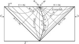
Figure 22: The Robinson-Trautman coordinates.

In the Robinson-Trautman coordinates ${{\mathfrak{u}},\,{\mathfrak{r}},\,\psi,\,\varphi}$ (or in their complex version ${{\mathfrak{u}},\,{\mathfrak{r}},\,\zeta,\,{\bar{\zeta}}}$), de Sitter metric takes the standard Robinson-Trautman form Stephani et al. (2002). The coordinate ${{\mathfrak{u}}}$ is null, the “radial” coordinate ${{\mathfrak{r}}}$ is an affine parameter along coordinate lines ${{\mathfrak{u}},\psi,\varphi=\text{constant}}$. These lines are null geodesics generating light cones with vertices at the origin ${{\mathfrak{r}}=0}$. The coordinates ${\psi,\,\varphi}$ (or ${\zeta,\,{\bar{\zeta}}}$) are angular coordinates, however, they are not functions of the accelerated angular coordinates ${{\vartheta^{\prime}},\varphi}$ only (cf. Eq. (246)). Because ${{\vartheta^{\prime}},\varphi}$ have a clearer geometrical meaning, we list some formulas also in the mixed coordinate system ${{\mathfrak{u}},\,{\mathfrak{r}},\,{\vartheta^{\prime}},\varphi}$.

The origin ${{\mathfrak{r}}=0}$ of the Robinson-Trautman coordinates is centered on the worldline of the uniformly accelerated observer moving with the acceleration ${\left\lvert a_{\mathrm{o}}\right\rvert=\left\lvert\ell_{\scriptscriptstyle\Lambda}^{\!-1}\sinh\alpha_{\mathrm{o}}\right\rvert}$. The coordinates are thus closely related to the accelerated coordinates.

The coordinates ${{\mathfrak{u}},\,{\mathfrak{r}},\,\psi,\,\varphi}$ do not cover the whole spacetime smoothly. They can be introduced smoothly in the future of the north pole, or in the past of the south pole. At the boundary of these two domains, ${{\mathfrak{u}}\to\pm\infty}$.

Metric and relation between coordinates

$${\mathrm{\mathit{g}}}=-H\,{\mathrm{\mathrm{d}}}{\mathfrak{u}}{}^{2}-{\mathrm{\mathrm{d}}}{\mathfrak{u}}\mathbin{\scriptstyle{\vee}}{\mathrm{\mathrm{d}}}{\mathfrak{r}}+\frac{{\mathfrak{r}}^{2}}{P^{2}}\,\bigl{(}{\mathrm{\mathrm{d}}}\psi{}^{2}+{\mathrm{\mathrm{d}}}\varphi{}^{2}\bigr{)}{\mbox{\;,}}$$ (241)

$${\mathrm{\mathit{g}}}=-H\,{\mathrm{\mathrm{d}}}{\mathfrak{u}}{}^{2}-{\mathrm{\mathrm{d}}}{\mathfrak{u}}\mathbin{\scriptstyle{\vee}}{\mathrm{\mathrm{d}}}{\mathfrak{r}}+\frac{{\mathfrak{r}}^{2}}{P^{2}}\,{\mathrm{\mathrm{d}}}\zeta\mathbin{\scriptstyle{\vee}}{\mathrm{\mathrm{d}}}{\bar{\zeta}}{\mbox{\;,}}$$ (242)

$$\begin{split}{\mathrm{\mathit{g}}}&=-\cosh^{2}\!\alpha_{\mathrm{o}}\,\frac{{\mathfrak{r}}^{2}}{\ell_{\scriptscriptstyle\Lambda}^{2}}\,(\upsilon^{2}-1)\,{\mathrm{\mathrm{d}}}{\mathfrak{u}}{}^{2}-{\mathrm{\mathrm{d}}}{\mathfrak{u}}\mathbin{\scriptstyle{\vee}}{\mathrm{\mathrm{d}}}{\mathfrak{r}}\\ &\quad+\cosh\alpha_{\mathrm{o}}\,\frac{{\mathfrak{r}}^{2}}{\ell_{\scriptscriptstyle\Lambda}}\,\sin{\vartheta^{\prime}}\,{\mathrm{\mathrm{d}}}{\mathfrak{u}}\mathbin{\scriptstyle{\vee}}{\mathrm{\mathrm{d}}}{\vartheta^{\prime}}+{\mathfrak{r}}^{2}\bigl{(}{\mathrm{\mathrm{d}}}{\vartheta^{\prime}}{}^{2}+\sin^{2}\!{\vartheta^{\prime}}\,{\mathrm{\mathrm{d}}}\varphi{}^{2}\bigr{)}{\mbox{\;,}}\end{split}$$ (243)

$$H =-\frac{{\mathfrak{r}}^{2}}{\ell_{\scriptscriptstyle\Lambda}^{2}}+2\,\frac{{\mathfrak{r}}}{\ell_{\scriptscriptstyle\Lambda}}\,\sinh\alpha_{\mathrm{o}}\,\tanh\Bigl{(}\psi-\frac{{\mathfrak{u}}}{\ell_{\scriptscriptstyle\Lambda}}\,\sinh\alpha_{\mathrm{o}}\Bigr{)}+1$$

$$=-\frac{{\mathfrak{r}}^{2}}{\ell_{\scriptscriptstyle\Lambda}^{2}}-2\,\frac{{\mathfrak{r}}}{\ell_{\scriptscriptstyle\Lambda}}\,\sinh\alpha_{\mathrm{o}}\,\cos{\vartheta^{\prime}}+1{\mbox{\;,}}$$ (244)

$$P =\cosh\Bigl{(}\psi-\frac{{\mathfrak{u}}}{\ell_{\scriptscriptstyle\Lambda}}\,\sinh\alpha_{\mathrm{o}}\Bigr{)}=\frac{1}{\sin{\vartheta^{\prime}}}{\mbox{\;.}}$$ (245)

$$\begin{gathered}\psi=\frac{{\mathfrak{u}}}{\ell_{\scriptscriptstyle\Lambda}}\,\sinh\alpha_{\mathrm{o}}+\log\left\lvert\tan\frac{{\vartheta^{\prime}}}{2}\right\rvert{\mbox{\;,}}\\ \left\lvert\tan\frac{{\vartheta^{\prime}}}{2}\right\rvert=\exp\Bigl{(}\psi-\frac{{\mathfrak{u}}}{\ell_{\scriptscriptstyle\Lambda}}\,\sinh\alpha_{\mathrm{o}}\Bigr{)}{\mbox{\;,}}\end{gathered}$$ (246)

$$\zeta=\frac{1}{\sqrt{2}}(\psi-i\varphi){\mbox{\;,}} \psi=\frac{1}{\sqrt{2}}(\zeta+{\bar{\zeta}}){\mbox{\;,}}$$ (247)

$${\bar{\zeta}}=\frac{1}{\sqrt{2}}(\psi+i\varphi){\mbox{\;,}} \varphi=\frac{i}{\sqrt{2}}(\zeta-{\bar{\zeta}}){\mbox{\;.}}$$

Null tetrad

Since the Robinson-Trautman coordinates are closely related to the congruence of null geodesics, it is convenient to introduce the null tetrad which is parallelly transported along these geodesics ${{\mathfrak{u}},\psi,\varphi=\text{constant}}$:

$$\begin{gathered}{{\mathrm{k}}}_{\scriptscriptstyle{\mathrm{RT}}}=\frac{1}{\sqrt{2}}{\frac{\partial}{\partial{\mathfrak{r}}}}{\mbox{\;,\quad}}{{\mathrm{l}}}_{\scriptscriptstyle{\mathrm{RT}}}=-\frac{1}{\sqrt{2}}H\,{\frac{\partial}{\partial{\mathfrak{r}}}}+\sqrt{2}\,{\frac{\partial}{\partial{\mathfrak{u}}}}{\mbox{\;,}}\\ {{\mathrm{m}}}_{\scriptscriptstyle{\mathrm{RT}}}=\frac{1}{\sqrt{2}}\,\frac{P}{{\mathfrak{r}}}\,\Bigl{(}{\frac{\partial}{\partial\psi}}-i{\frac{\partial}{\partial\varphi}}\Bigr{)}{\mbox{\;,}}\\ {\bar{{\mathrm{m}}}}_{\scriptscriptstyle{\mathrm{RT}}}=\frac{1}{\sqrt{2}}\,\frac{P}{{\mathfrak{r}}}\,\Bigl{(}{\frac{\partial}{\partial\psi}}+i{\frac{\partial}{\partial\varphi}}\Bigr{)}{\mbox{\;.}}\end{gathered}$$ (248)

Relation to accelerated coordinate family

$${\mathfrak{r}} =\frac{{R^{\prime}}{}\sqrt{1-{R_{\mathrm{o}}^{2}}/{\ell_{\scriptscriptstyle\Lambda}^{2}}}}{1+({{R^{\prime}}{}R_{\mathrm{o}}}/{\ell_{\scriptscriptstyle\Lambda}^{2}})\cos{\vartheta^{\prime}}}{\mbox{\;,}}$$ (249)

$${\mathfrak{u}} =\sqrt{1-\frac{R_{\mathrm{o}}^{2}}{\ell_{\scriptscriptstyle\Lambda}^{2}}}\,\Biggl{(}{T^{\prime}}{}+\frac{\ell_{\scriptscriptstyle\Lambda}}{2}\log\left\lvert\frac{{R^{\prime}}{}-\ell_{\scriptscriptstyle\Lambda}}{{R^{\prime}}{}+\ell_{\scriptscriptstyle\Lambda}}\right\rvert\Biggr{)}{\mbox{\;,}}$$

$$\psi =\frac{R_{\mathrm{o}}}{\ell_{\scriptscriptstyle\Lambda}}\,\Biggl{(}\frac{{T^{\prime}}{}}{\ell_{\scriptscriptstyle\Lambda}}+\frac{1}{2}\log\left\lvert\frac{{R^{\prime}}{}-\ell_{\scriptscriptstyle\Lambda}}{{R^{\prime}}{}+\ell_{\scriptscriptstyle\Lambda}}\right\rvert\Biggr{)}+\log\left\lvert\tan\frac{{\vartheta^{\prime}}}{2}\right\rvert\!\!{\mbox{\;,}}\!\!$$

$${\mathfrak{r}} =\frac{\ell_{\scriptscriptstyle\Lambda}}{\upsilon\cosh\alpha_{\mathrm{o}}-\xi\sinh\alpha_{\mathrm{o}}}{\mbox{\;,}}$$

$${\mathfrak{u}} =\frac{\ell_{\scriptscriptstyle\Lambda}}{\cosh\alpha_{\mathrm{o}}}\Biggl{(}\tau+\frac{1}{2}\log\left\lvert\frac{1-\upsilon}{1+\upsilon}\right\rvert\Biggr{)}{\mbox{\;,}}$$ (250)

$$\psi =\tanh\alpha_{\mathrm{o}}\Biggl{(}\tau+\frac{1}{2}\log\left\lvert\frac{1-\upsilon}{1+\upsilon}\right\rvert\Biggr{)}+\frac{1}{2}\log\left\lvert\frac{1+\xi}{1-\xi}\right\rvert{\mbox{\;.}}$$

Relation to static family

$${\mathfrak{r}}\!=\!\frac{\ell_{\scriptscriptstyle\Lambda}}{\sqrt{1{-}R_{\mathrm{o}}^{2}/\ell_{\scriptscriptstyle\Lambda}^{2}}}\biggl{[}\Bigl{(}1{-}\frac{RR_{\mathrm{o}}}{\ell_{\scriptscriptstyle\Lambda}^{2}}\cos\vartheta\Bigr{)}^{2}\!{-}\Bigl{(}1{-}\frac{R^{2}}{\ell_{\scriptscriptstyle\Lambda}^{2}}\Bigr{)}\Bigl{(}1{-}\frac{R_{\mathrm{o}}^{2}}{\ell_{\scriptscriptstyle\Lambda}^{2}}\Bigr{)}\biggr{]}^{\!\frac{1}{2}}\!\!{\mbox{\;,}}$$ (251)

$${\mathfrak{r}}\sin{\vartheta^{\prime}} =R\sin\vartheta{\mbox{\;,\quad}}{\mathfrak{r}}\cos{\vartheta^{\prime}} =\frac{R\cos\vartheta-R_{\mathrm{o}}}{\sqrt{1-R_{\mathrm{o}}^{2}/\ell_{\scriptscriptstyle\Lambda}^{2}}}{\mbox{\;.}}$$ (252)

$$R\sin\vartheta ={\mathfrak{r}}\sin{\vartheta^{\prime}}{\mbox{\;,}}$$ (253)

$$R\cos\vartheta ={\mathfrak{r}}\cos{\vartheta^{\prime}}\sqrt{1-{R_{\mathrm{o}}^{2}}/{\ell_{\scriptscriptstyle\Lambda}^{2}}}+R_{\mathrm{o}}{\mbox{\;.}}$$

A.10 The null family

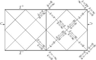
Figure 23: The null family of coordinates

Finally, we return back to the coordinate systems which employ standard coordinates ${\vartheta}$, ${\varphi}$. Time and radial coordinates can be transformed into two null coordinates. Such null coordinates can be associated with most coordinate families introduced above. Coordinates ${{\tilde{u}},\,{\tilde{v}}}$ are related to the standard coordinates; ${{\check{u}},\,{\check{v}}}$ and ${{\hat{u}},\,{\hat{v}}}$ to the flat cosmological coordinates; ${u,\,v}$ to the conformally Minkowski; and ${{\bar{u}},\,{\bar{v}}}$ to the static coordinates. Coordinate vectors ${\{{{\partial}/{\partial{\tilde{u}}}},\,{{\partial}/{\partial{\tilde{v}}}}\}}$, ${\{{{\partial}/{\partial{\check{u}}}},\,{{\partial}/{\partial{\check{v}}}}\}}$, etc., are the pairs of independent null vectors in the radial 2-slices ${\vartheta,\varphi=\text{constant}}$. We do not allow the radial coordinate to be negative in the definitions of null coordinates because this would interchange the meaning of ${u}$ and ${v}$. The null coordinates are thus drawn in the right half of Fig. 23 only.

Metric and relation to other coordinates

$${\mathrm{\mathit{g}}}=\frac{\ell_{\scriptscriptstyle\Lambda}^{2}}{1-\cos({\tilde{u}}+{\tilde{v}})}\Bigl{(}-{\mathrm{\mathrm{d}}}{\tilde{u}}\mathbin{\scriptstyle{\vee}}{\mathrm{\mathrm{d}}}{\tilde{v}}+\bigl{(}1-\cos({\tilde{u}}-{\tilde{v}})\bigr{)}\,{{\mathrm{\mathrm{d}\omega}}^{2}}\Bigr{)}{\mbox{\;,}}$$ (254)

$${\mathrm{\mathit{g}}}=\frac{\ell_{\scriptscriptstyle\Lambda}^{2}}{({\hat{u}}+{\hat{v}})^{2}}\,\Bigl{(}-2\,{\mathrm{\mathrm{d}}}{\hat{u}}\mathbin{\scriptstyle{\vee}}{\mathrm{\mathrm{d}}}{\hat{v}}+({\hat{u}}-{\hat{v}})^{2}\,{{\mathrm{\mathrm{d}\omega}}^{2}}\Bigr{)}{\mbox{\;,\quad}}$$ (255)

$${\mathrm{\mathit{g}}}=\frac{\ell_{\scriptscriptstyle\Lambda}^{2}}{({\check{u}}+{\check{v}})^{2}}\,\Bigl{(}-2\,{\mathrm{\mathrm{d}}}{\check{u}}\mathbin{\scriptstyle{\vee}}{\mathrm{\mathrm{d}}}{\check{v}}+({\check{u}}-{\check{v}})^{2}\,{{\mathrm{\mathrm{d}\omega}}^{2}}\Bigr{)}{\mbox{\;,\quad}}\,$$ (256)

$${\mathrm{\mathit{g}}}=\Bigl{(}\frac{\ell_{\scriptscriptstyle\Lambda}^{2}}{\ell_{\scriptscriptstyle\Lambda}^{2}-uv}\Bigr{)}^{2}\,\Bigl{(}-2\,{\mathrm{\mathrm{d}}}u\mathbin{\scriptstyle{\vee}}{\mathrm{\mathrm{d}}}v+(u-v)^{2}\,{{\mathrm{\mathrm{d}\omega}}^{2}}\Bigr{)}{\mbox{\;,}}$$ (257)

$$\begin{split}&{\mathrm{\mathit{g}}}=\Bigl{(}\exp\frac{{\bar{u}}}{\ell_{\scriptscriptstyle\Lambda}}+\exp\frac{{\bar{v}}}{\ell_{\scriptscriptstyle\Lambda}}\Bigr{)}^{\!\!-2}\\ &\,\times\!\!\Biggl{(}-2\exp\frac{{\bar{u}}+{\bar{v}}}{\ell_{\scriptscriptstyle\Lambda}}\,{\mathrm{\mathrm{d}}}{\bar{u}}\mathbin{\scriptstyle{\vee}}{\mathrm{\mathrm{d}}}{\bar{v}}+\ell_{\scriptscriptstyle\Lambda}^{2}\,\Bigl{(}\exp\frac{{\bar{u}}}{\ell_{\scriptscriptstyle\Lambda}}-\exp\frac{{\bar{v}}}{\ell_{\scriptscriptstyle\Lambda}}\Bigr{)}^{2}\,{{\mathrm{\mathrm{d}\omega}}^{2}}\Biggr{)}\!{\mbox{\;.}}\end{split}$$ (258)

The relation of time and radial coordinates ${\overstar{t},\,\overstar{r}}$ to the corresponding null coordinates ${\overstar{u},\,\overstar{v}}$ is given by usual formulas:

$$\begin{gathered}\overstar{t}={\textstyle\frac{1}{2}}(\overstar{v}+\overstar{u}){\mbox{\;,\quad}}\overstar{u}=\overstar{t}-\overstar{r}{\mbox{\;,}}\\ \overstar{r}={\textstyle\frac{1}{2}}(\overstar{v}-\overstar{u}){\mbox{\;,\quad}}\overstar{v}=\overstar{t}+\overstar{r}{\mbox{\;.}}\end{gathered}$$ (259)

Here ${\{\overstar{t},\,\overstar{r}\}}$ stands for ${\{{\tilde{t}},\,{\tilde{r}}\}}$, ${\{{\check{t}},\,{\check{r}}\}}$, ${\{{\hat{t}},\,{\hat{r}}\}}$, ${\{t,\,r\}}$, and ${\{{\bar{t}},\,{\bar{r}}\}}$ respectively; similarly with ${\{\overstar{u},\,\overstar{v}\}}$.

Relation between null coordinates

The coordinates ${{\hat{u}},\,{\hat{v}}}$,  ${u,\,v}$, and ${{\check{u}},\,{\check{v}}}$ can be viewed as null coordinates in the conformally related Minkowski spaces ${\hat{M}}$, ${M}$, and ${\check{M}}$; these are shifted with respect to each other by ${\frac{\pi}{2}}$ in the direction of the conformally Einstein time coordinate ${{\tilde{t}}}$, or associated null coordinates:

$$\frac{{\hat{u}}}{\ell_{\scriptscriptstyle\Lambda}} =\tan\frac{{\tilde{u}}}{2}{\mbox{\;,}} \frac{{\hat{v}}}{\ell_{\scriptscriptstyle\Lambda}} =\tan\frac{{\tilde{v}}}{2}{\mbox{\;,}}$$ (260)

$$\frac{u}{\ell_{\scriptscriptstyle\Lambda}} =\tan\Bigl{(}\frac{{\tilde{u}}}{2}-\frac{\pi}{4}\Bigr{)}{\mbox{\;,}} \frac{v}{\ell_{\scriptscriptstyle\Lambda}} =\tan\Bigl{(}\frac{{\tilde{v}}}{2}-\frac{\pi}{4}\Bigr{)}{\mbox{\;,}}$$

$$\frac{{\check{u}}}{\ell_{\scriptscriptstyle\Lambda}} =\tan\Bigl{(}\frac{{\tilde{u}}}{2}-\frac{\pi}{2}\Bigr{)}{\mbox{\;,}} \frac{{\check{v}}}{\ell_{\scriptscriptstyle\Lambda}} =\tan\Bigl{(}\frac{{\tilde{v}}}{2}-\frac{\pi}{2}\Bigr{)}{\mbox{\;.}}$$

The remaining coordinates ${{\bar{u}},\,{\bar{v}}}$ are related to the conformally Einstein null coordinates ${{\tilde{u}},\,{\tilde{v}}}$ by the “compactification transformation”:

$$\tan\frac{{\tilde{u}}}{2}={s_{u}}\exp\frac{{\bar{u}}}{\ell_{\scriptscriptstyle\Lambda}}{\mbox{\;,\quad}}\tan\frac{{\tilde{v}}}{2}={s_{v}}\exp\frac{{\bar{v}}}{\ell_{\scriptscriptstyle\Lambda}}{\mbox{\;.}}$$ (261)

Here the sign factors ${{s_{u}}}$ and ${{s_{v}}}$ are given by

$${s_{u}}=\operatorname{sign}\tan\frac{{\tilde{u}}}{2}{\mbox{\;,\quad}}{s_{v}}=\operatorname{sign}\tan\frac{{\tilde{v}}}{2}{\mbox{\;.}}$$ (262)

Relations (260), (261) between null coordinates can also be rewritten as follows:

$$\tan\frac{{\tilde{u}}}{2}={s_{u}}\exp\frac{{\bar{u}}}{\ell_{\scriptscriptstyle\Lambda}}=\frac{{\hat{u}}}{\ell_{\scriptscriptstyle\Lambda}}=-\frac{\ell_{\scriptscriptstyle\Lambda}}{{\check{u}}}=\frac{\ell_{\scriptscriptstyle\Lambda}+u}{\ell_{\scriptscriptstyle\Lambda}-u}{\mbox{\;,}}$$ (263)

$$\tan{\tilde{u}}=-{s_{u}}\sinh^{\!-1}\!\frac{{\bar{u}}}{\ell_{\scriptscriptstyle\Lambda}}=\frac{2{\hat{u}}\ell_{\scriptscriptstyle\Lambda}}{\ell_{\scriptscriptstyle\Lambda}^{2}-{\hat{u}}^{2}}=\frac{2{\check{u}}\ell_{\scriptscriptstyle\Lambda}}{\ell_{\scriptscriptstyle\Lambda}^{2}-{\check{u}}^{2}}=\frac{u^{2}-\ell_{\scriptscriptstyle\Lambda}^{2}}{2u\ell_{\scriptscriptstyle\Lambda}}\!{\mbox{\;,}}$$

$$\sin{\tilde{u}}={s_{u}}\cosh^{\!-1}\!\frac{{\bar{u}}}{\ell_{\scriptscriptstyle\Lambda}}=\frac{2{\hat{u}}\ell_{\scriptscriptstyle\Lambda}}{\ell_{\scriptscriptstyle\Lambda}^{2}+{\hat{u}}^{2}}=\frac{-2{\check{u}}\ell_{\scriptscriptstyle\Lambda}}{\ell_{\scriptscriptstyle\Lambda}^{2}+{\check{u}}^{2}}=\frac{\ell_{\scriptscriptstyle\Lambda}^{2}-u^{2}}{\ell_{\scriptscriptstyle\Lambda}^{2}+u^{2}}{\mbox{\;,}}$$

$$\cos{\tilde{u}}=-\tanh\frac{{\bar{u}}}{\ell_{\scriptscriptstyle\Lambda}}=\frac{\ell_{\scriptscriptstyle\Lambda}^{2}-{\hat{u}}^{2}}{\ell_{\scriptscriptstyle\Lambda}^{2}+{\hat{u}}^{2}}=\frac{{\hat{u}}^{2}-\ell_{\scriptscriptstyle\Lambda}^{2}}{{\hat{u}}^{2}+\ell_{\scriptscriptstyle\Lambda}^{2}}=\frac{-2u\ell_{\scriptscriptstyle\Lambda}}{\ell_{\scriptscriptstyle\Lambda}^{2}+u^{2}}{\mbox{\;,}}$$

$$\frac{{\hat{u}}}{\ell_{\scriptscriptstyle\Lambda}}=\tan\frac{{\tilde{u}}}{2}={s_{u}}\exp\frac{{\bar{u}}}{\ell_{\scriptscriptstyle\Lambda}}=-\frac{\ell_{\scriptscriptstyle\Lambda}}{{\check{u}}}=\frac{\ell_{\scriptscriptstyle\Lambda}+u}{\ell_{\scriptscriptstyle\Lambda}-u}{\mbox{\;,}}$$ (264)

$$-\frac{{\check{u}}}{\ell_{\scriptscriptstyle\Lambda}}=\cot\frac{{\tilde{u}}}{2}={s_{u}}\exp\Bigl{(}-\frac{{\bar{u}}}{\ell_{\scriptscriptstyle\Lambda}}\Bigr{)}=\frac{\ell_{\scriptscriptstyle\Lambda}}{{\hat{u}}}=\frac{\ell_{\scriptscriptstyle\Lambda}-u}{\ell_{\scriptscriptstyle\Lambda}+u}{\mbox{\;,}}$$ (265)

$$\frac{u}{\ell_{\scriptscriptstyle\Lambda}} =-\frac{1-\sin{\tilde{u}}}{\cos{\tilde{u}}}=-\frac{\cos{\tilde{u}}}{1+\sin{\tilde{u}}}$$ (266)

$$=\Bigl{(}\tanh\frac{{\bar{u}}}{2\ell_{\scriptscriptstyle\Lambda}}\Bigr{)}^{s_{u}}=\frac{{\hat{u}}-\ell_{\scriptscriptstyle\Lambda}}{{\hat{u}}+\ell_{\scriptscriptstyle\Lambda}}=\frac{\ell_{\scriptscriptstyle\Lambda}+{\check{u}}}{\ell_{\scriptscriptstyle\Lambda}-{\check{u}}}{\mbox{\;,}}$$

$$\frac{{\bar{u}}}{\ell_{\scriptscriptstyle\Lambda}} =\log\left\lvert\tan\frac{{\tilde{u}}}{2}\right\rvert=\log\left\lvert\frac{{\hat{u}}}{\ell_{\scriptscriptstyle\Lambda}}\right\rvert=\log\left\lvert\frac{\ell_{\scriptscriptstyle\Lambda}}{{\check{u}}}\right\rvert$$ (267)

$$=\log\left\lvert\frac{\ell_{\scriptscriptstyle\Lambda}+u}{\ell_{\scriptscriptstyle\Lambda}-u}\right\rvert=2\operatorname{arctanh}\Bigl{(}\frac{u}{\ell_{\scriptscriptstyle\Lambda}}\Bigr{)}^{s_{u}}{\mbox{\;.}}$$

$${\hat{u}}{\check{u}}=-\ell_{\scriptscriptstyle\Lambda}^{2}{\mbox{\;,\quad}}\frac{{\hat{u}}}{\ell_{\scriptscriptstyle\Lambda}}+\frac{\ell_{\scriptscriptstyle\Lambda}}{{\check{u}}}=0{\mbox{\;.}}$$ (268)

The same relations hold for coordinates ${v}$.

References

- Born (1909) M. Born, Ann. Phys. (Leipzig) 30, 1 (1909).
- Ginzburg (1970) V. L. Ginzburg, Soviet Physics Uspekhi 12, 565 (1970).
- Ginzburg (1979) V. L. Ginzburg, Theoretical Physics and Astrophysics (Pergamon Press, Oxford, 1979).
- Ginzburg (1989) V. L. Ginzburg, Applications of Electrodynamics in Theoretical Physics and Astrophysics (Gordon and Breach, New York, 1989).
- Bondi (1981) H. Bondi, Proc. R. Soc. Lond., Ser A 376, 493 (1981).
- Boulware (1980) D. G. Boulware, Ann. Phys. (N.Y.) 124, 169 (1980).
- Peierls (1979) R. Peierls, in Surprises in Theoretical Physics (Princeton University Press, Princeton, 1979).
- Thirring (1986) W. Thirring, A Course in Mathematical Physics II: Classical Field Theory (Springer, New York, Wien, 1986).
- Herrera (1983) L. Herrera, Il Nuov. Cim. 78B, 156 (1983).
- Harpaz and Soker (1998) A. Harpaz and N. Soker, Gen. Rel. Grav. 30, 1217 (1998).
- Gupta and Padmanabhan (1998) A. Gupta and T. Padmanabhan, Phys. Rev. D 57, 7241 (1998).
- Shariati and Khorrami (1999) A. Shariati and M. Khorrami, Found. Phys. Lett. 12, 427 (1999).
- Bičák and Muschall (1990) J. Bičák and R. Muschall, Wiss. Zeits. der Friedrich-Schiller-Universität Jena 39, 1827 (1990).
- Eriksen and Grøn (2000a) E. Eriksen and Ø. Grøn, Ann. Phys. (N.Y.) 286, 320 (2000a).
- Eriksen and Grøn (2000b) E. Eriksen and Ø. Grøn, Ann. Phys. (N.Y.) 286, 343 (2000b).
- Eriksen and Grøn (2000c) E. Eriksen and Ø. Grøn, Ann. Phys. (N.Y.) 286, 373 (2000c).
- Bičák and Schmidt (1989) J. Bičák and B. G. Schmidt, Phys. Rev. D 40, 1827 (1989). See in particular Section IVB and Appendix A there, but beware that the conventions we are using here are different to comply with the conventions used in Bičák and Krtouš (2001, 2002).
- Bičák (2000) J. Bičák, Selected Solutions of Einstein’s Field Equations: Their Role in General Relativity and Astrophysics, in Einstein’s Field Equations and Their Physical Implications (Selected Essays in Honour of Jürgen Ehlers), edited by B. G. Schmidt, Lecture Notes in Physics 540 (Springer, Berlin, 2000), pp. 1–126, eprint gr-qc/0004016.
- Bičák and Krtouš (2003) J. Bičák and P. Krtouš, in Recent Developments in Gravity (Proceedings of 10th Greek Relativity Meeting, Chalkidiki, May 2002), edited by K. D. Kokkotas and N. Stergioulas (World Scientific, Singapore, 2003), pp. 3–25, eprint gr-qc/0303091.
- Pravda and Pravdová (2000) V. Pravda and A. Pravdová, Czech. J. Phys. 50, 333 (2000), eprint gr-qc/0003067.
- Penrose (1965) R. Penrose, Proc. R. Soc. Lond., Ser A 284, 159 (1965).
- Maeda (1989) K. Maeda, in Proceedings of the Fifth M. Grossman Meeting on General Relativity, Perth, Australia, 1988, edited by D. G. Blair, M. J. Buckingham, and R. Ruffini (World Scientific, Singapore, 1989).
- Rendall (2004) A. D. Rendall, Ann. H. Poincaré 5, 1041 (2004), eprint gr-qc/0312020.
- Bičák and Krtouš (2001) J. Bičák and P. Krtouš, Phys. Rev. D 64, 124020 (2001), eprint gr-qc/0107078.
- Bičák and Krtouš (2002) J. Bičák and P. Krtouš, Phys. Rev. Lett. 88, 211101 (2002), eprint gr-qc/0207010.
- Krtouš et al. (2003) P. Krtouš, J. Podolský, and J. Bičák, Phys. Rev. Lett. 91, 061101 (2003), eprint gr-qc/0308004.
- Krtouš and Podolský (2003) P. Krtouš and J. Podolský, Phys. Rev. D 68, 024005 (2003), eprint gr-qc/0301110.
- Podolský et al. (2003) J. Podolský, M. Ortaggio, and P. Krtouš, Phys. Rev. D 68, 124004 (2003), eprint gr-qc/0307108. The coordinates differ from the “standard” coordinates of Kinnersley and Walker (1970) (where only case is considered) by a simple rescaling , , and . The conformal factor is then given by .
- Dias and Lemos (2003a) O. J. C. Dias and J. P. S. Lemos, Phys. Rev. D 67, 084018 (2003a), eprint hep-th/0301046.
- Dias and Lemos (2003b) O. J. C. Dias and J. P. S. Lemos, Phys. Rev. D 67, 064001 (2003b), eprint hep-th/0210065.
- Krtouš and Podolský (2004) P. Krtouš and J. Podolský, Phys. Rev. D 69, 084023 (2004), eprint gr-qc/0310089.
- Einstein (1907) A. Einstein, Jahrb. d. Radioaktivität u. Elektronik 4, 411 (1907).
- Einstein (1908) A. Einstein, Jahrb. d. Radioaktivität u. Elektronik 5, 98 (1908).
- Rohrlich (1965) F. Rohrlich, Classical Charged Particles (Addison-Wesley, Reading, 1965).
- Hill (1945) E. L. Hill, Phys. Rev. 67, 358 (1945).
- Hill (1947) E. L. Hill, Phys. Rev. 72, 143 (1947).
- Fulton and Rohrlich (1960) T. Fulton and F. Rohrlich, Ann. Phys. (N.Y.) 9, 499 (1960).
- Leibovitz and Peres (1963) C. Leibovitz and A. Peres, Ann. Phys. (N.Y.) 25, 400 (1963).
- Bondi and Gold (1955) H. Bondi and T. Gold, Proc. R. Soc. Lond., Ser A 229, 416 (1955).
- Krtouš (1991) P. Krtouš, Physical fields of uniformly accelerated sources, Master thesis (Charles University, Prague, Czechoslovakia, 1991), in Czech.
- Schmidt (1993) H. J. Schmidt, Fortschr. d. Physik 41, 179 (1993).
- Eriksen and Grøn (1995) E. Eriksen and Ø. Grøn, Int. J. Mod. Phys. D4, 115 (1995).
- Rindler (2001) W. Rindler, Relativity: special, general, and cosmological (Oxford University Press, Oxford, 2001).
- Penrose (1968) R. Penrose, in Battelle Recontres, edited by B. DeWitt and J. A. Wheeler (Benjamin, New York, 1968), pp. 121–235.
- Penrose and Rindler (1984, 1986) R. Penrose and W. Rindler, Spinors and Space-Time (Cambridge University Press, Cambridge, England, 1984, 1986).
- Hawking and Ellis (1973) S. W. Hawking and G. F. R. Ellis, The Large Scale Structure of Space-Time (Cambridge University Press, Cambridge, England, 1973).
- Wald (1984) R. M. Wald, General Relativity (The University of Chicago Press, Chicago and London, 1984).
- Cvetič et al. (1993) M. Cvetič, S. Griffies, and H. H. Soleng, Phys. Rev. D 48, 2613 (1993).
- Podolský and Griffiths (2001) J. Podolský and J. B. Griffiths, Phys. Rev. D 63, 024006 (2001), eprint gr-qc/0010109.
- Stephani et al. (2002) H. Stephani, D. Kramer, M. Maccallum, C. Hoenselaers, and E. Herlt, Exact Solutions of Einstein’s Field Equations, Second Edition (Cambridge University Press, Cambridge, England, 2003).
- Bondi et al. (1962) H. Bondi, M. G. J. van der Burg, and A. W. K. Metzner, Proc. R. Soc. Lond., Ser A 269, 21 (1962).
- (52) For the detailed derivation, see Bičák and Krtouš (2001), Section V. The field (87), with given by (89), is the field (5.2) in Bičák and Krtouš (2001). Notice, however, the following changes in notation: the quantities , and in Bičák and Krtouš (2001) are, in the present paper, denoted by , and with again given by Eq. (54). Since the field (87) (as well as the electromagnetic field (90)) can be written as a symmetric combination of retarded and advanced effects from both charges, we called it “symmetric” in Bičák and Krtouš (2001) and used a subscript “sym”. Such a notation was necessary in Ref. Bičák and Krtouš (2001), but is not used here.
- Bičák (1968) J. Bičák, Proc. R. Soc. Lond., Ser A 302, 201 (1968).
- Pauli (1958) W. Pauli, Theory of Relativity (Pergamon Press, London, 1958).
- Jackson (1975) J. D. Jackson, Classical Electrodynamics (J. Wiley, New York, London, 1975).
- Goldberg and Kerr (1964) J. N. Goldberg and R. P. Kerr, J. Math. Phys. 5, 172 (1964).
- Riess etal (2004) A. G. Riess et al (20 authors), Ap. J. 607, 665 (2004).
- Woodard (2004) R. P. Woodard, in Deserfest: A celebration of the life and works of Stanley Deser edited by J. T. Liu and K. Stelle (World Scientific, New Jersey, London, Singapore, 2005), eprint gr-qc/0408002.
- Kinnersley and Walker (1970) W. Kinnersley and M. Walker, Phys. Rev. D 2, 1359 (1970).