Fermion Mass Generation in de Sitter Space

Abstract

We study the one-loop radiative corrections for massless fermions in de Sitter space induced by a Yukawa coupling to a light, nearly minimally coupled scalar field. We show that the fermions acquire a mass. Next we construct the corresponding (nonlocal) effective fermionic action, which – in contrast to the case of a massive Dirac fermion – preserves chirality. Nevertheless, the resulting fermion dynamics is precisely that of a Dirac fermion with a mass proportional to the expansion rate. Our finding supports the view that an observer or a test particle responds to a scalar field in inflation by shifting its energy rather than seeing a thermal bath.

I Introduction

The question of the dynamics of fermions interacting through a Yukawa coupling with a massless minimally coupled scalar field in de Sitter space was originally considered in Ref. ProkopecWoodard:2003 . It is the simplest nontrivial example allowing for a one loop study of quantum effects during inflation. Here we reconsider the problem, by assuming that the scalar field is light and nearly minimally coupled, which allows us to calculate radiative corrections employing a de Sitter invariant scalar propagator. We make substantial analytic progress, such that some of the questions that were left unanswered in the original work, e.g. the problem of Pauli blocking and vector current conservation, are resolved.

Gaining analytical understanding of fermion dynamics during inflation may have important cosmological ramifications, in particular for baryogenesis and the origin of dark matter in the Universe. Closely related are effects in massless scalar quantum electrodynamics, which may be of relevance for cosmic magnetogenesis Prokopec:PhotonMass ; ProkopecPuchwein:2003 , and of graviton induced self energy MiaoWoodard:2005 in de Sitter space.

On a more conceptual level, quantum theory in de Sitter space is most commonly considered in the context of horizon thermodynamics, which is locally witnessed by an Unruh detector at a response rate corresponding to thermal radiation GibbonsHawking:1977 ; GarbrechtProkopec:2004b . In recent work, we argued however that local effects predominantly become manifest in a shift of the detector’s energy levels GarbrechtProkopec:2005 . Since the Unruh detector is an idealised device, it is of interest what a test particle in a proper field-theoretic setting experiences, in particular whether effects similar to those of a thermal bath are present.

II One-Loop Self Energy

Massless fermions are conformally invariant, such that in a $D$-dimensional spacetime with the metric

$$ds^{2}=a^{2}\left(-d\eta^{2}+d\mathbf{x}^{2}\right)\,,$$ (1)

their propagator arises from a conformal rescaling of the flat-space counterpart

$${\rm i}S(x;x^{\prime})=(aa^{\prime})^{\frac{1-D}{2}}{\rm i}{\partial\!\!\!/}\left\{\frac{\Gamma\left(\frac{D}{2}-1\right)}{4\pi^{\frac{D}{2}}}\left[\Delta x^{2}(x;x^{\prime})\right]^{1-\frac{D}{2}}\right\}=-\frac{\Gamma\left(\frac{D}{2}\right)}{2\pi^{\frac{D}{2}}}\frac{(aa^{\prime})^{\frac{1-D}{2}}{\rm i}\gamma^{\mu}\Delta x_{\mu}}{\left[\Delta x^{2}(x;x^{\prime})\right]^{\frac{D}{2}}}\,,$$ (2)

where $\Delta x^{2}=-(|\eta-\eta^{\prime}|-{\rm i}\epsilon)^{2}+\|\vec{x}-\vec{x}^{\,\prime}\|^{2}$ and $\Delta x_{\mu}=x_{\mu}-x^{\,\prime}_{\mu}$.

De Sitter space is endowed with the scale factor

$$a=-\frac{1}{H\eta}\,,$$ (3)

where $H$ denotes the Hubble parameter and $\eta$ conformal time. The Green function for a light nearly minimally coupled scalar in de Sitter space is of the following de Sitter invariant form ChernikovTagirov:1968 ,

$${\rm i}\Delta(x,x^{\prime})=\frac{\Gamma(\frac{D-1}{2}+\nu_{D})\Gamma(\frac{D-1}{2}-\nu_{D})}{(4\pi)^{\frac{D}{2}}\Gamma(\frac{D}{2})}H^{D-2}\;{}_{2}F_{1}\Big{(}\frac{D-1}{2}+\nu_{D},\frac{D-1}{2}-\nu_{D},\frac{D}{2},1-\frac{y}{4}\Big{)}\,,$$ (4)

where

$$\nu_{D}=\left[\left(\frac{D-1}{2}\right)^{2}-\frac{m^{2}+\xi R_{D}}{H^{2}}\right]^{\frac{1}{2}}\,,$$ (5)

$m$ is the mass of the scalar field, $R_{D}=D(D-1)H^{2}$ denotes the Ricci scalar curvature of de Sitter space, and $\xi$ is the coupling constant of the scalar field to curvature ($\xi=1/6$ corresponds to conformal coupling, $\xi=0$ to minimal coupling). The function $y=y(x;x^{\prime})$ is related to the de Sitter invariant length, $\ell=\ell(x;x^{\prime})$, as follows:

$$y = 4\sin^{2}\Big{(}\frac{1}{2}H\ell\Big{)}=aa^{\prime}H^{2}\Delta x^{2}\,,$$ (6)

$$\Delta x^{2} = -(|\eta-\eta^{\prime}|^{2}-i\epsilon)^{2}+\|\vec{x}-\vec{x}^{\,\prime}\|^{2}\,,$$ (7)

where $a\equiv a(\eta)=-1/(H\eta)$, $a^{\prime}\equiv a(\eta^{\prime})=-1/(H\eta^{\prime})$.

If $m^{2}+\xi R_{D}=0$, the Green function (4) is ill-defined. When attempting to calculate it by performing the momentum-sum over the modes, one sees that this problem corresponds to an infrared divergence TsamisWoodard:1993 , which has to be regulated. There exists no de Sitter invariant regulator Allen:1985 , which implies that there is no de Sitter invariant Green function for a massless minimally coupled scalar field. In a work on scalar electrodynamics in de Sitter space ProkopecPuchwein:2003 , the use of a de Sitter invariant propagator with a small mass or weak coupling $\xi$ to gravity was used in studying radiatively induced photon mass generation in de Sitter space. Here, we adapt this method to study the fermion dynamics in de Sitter background.

Since we are primarily interested in considering a small scalar mass and weak coupling to gravity,

$$m^{2}+\xi R_{D}\ll H^{2},$$ (8)

we find the following representation of the scalar propagator useful (cf. also Ref. ProkopecPuchwein:2003 ):

$${\rm i}\Delta(x;x^{\prime}) = \frac{H^{D-2}}{(4\pi)^{\frac{D}{2}}}\frac{\Gamma\Big{(}\frac{D}{2}\Big{)}\Gamma\Big{(}1-\frac{D}{2}\Big{)}}{\Gamma\Big{(}\frac{1}{2}+\nu_{D}\Big{)}\Gamma\Big{(}\frac{1}{2}-\nu_{D}\Big{)}}\Bigg{\{}\sum_{n=0}^{\infty}\frac{\Gamma\Big{(}\frac{D-1}{2}+\nu_{D}+n\Big{)}\Gamma\Big{(}\frac{D-1}{2}-\nu_{D}+n\Big{)}}{\Gamma\Big{(}\frac{D}{2}+n\Big{)}\Gamma\big{(}n+1\big{)}}\bigg{(}\frac{y}{4}\bigg{)}^{n}$$

$$\hskip 136.5733pt-\sum_{n=-1}^{\infty}\frac{\Gamma\Big{(}\frac{3}{2}+\nu_{D}+n\Big{)}\Gamma\Big{(}\frac{3}{2}-\nu_{D}+n\Big{)}}{\Gamma\Big{(}3-\frac{D}{2}+n\Big{)}\Gamma\big{(}n+2\big{)}}\bigg{(}\frac{y}{4}\bigg{)}^{n-\frac{D}{2}+2}\Bigg{\}}\,.$$

Notice that the conformal propagator corresponds to the $n=-1$ term of the second series (containing the $D$-dependent powers of $y$). We have recast the scalar propagator into the form (II), such that the cancellation of all terms $n\geq 0$ is manifest in $D=4$. The cancellation occurs only to leading order in an expansion around $D=4$ however. Since the prefactor is singular at $D=4$, the true and finite result in $D=4$ is obtained when the series are expanded to linear order in $D-4$, resulting in coefficients that are suppressed by $(m^{2}+\xi R_{D})/H^{2}\ll 1$, as we show below. The explicit form for the propagator that is suitable for this problem is thus ($\nu=\big{[}(3/2)^{2}-(m^{2}+\xi R)/H^{2}\big{]}^{1/2}$),

$${\rm i}\Delta(x;x^{\prime}) = \frac{H^{D-2}}{4\pi^{D/2}}\Gamma\Big{(}\frac{D}{2}-1\Big{)}\frac{1}{y^{\frac{D}{2}-1}}$$ (10)

$$+ \!\frac{H^{2}}{16\pi^{2}}\sum_{n=0}^{\infty}\frac{\Gamma\Big{(}\frac{3}{2}+\nu+n\Big{)}\Gamma\Big{(}\frac{3}{2}-\nu+n\Big{)}}{\Gamma\Big{(}\frac{1}{2}+\nu\Big{)}\Gamma\Big{(}\frac{1}{2}-\nu\Big{)}}\bigg{(}\frac{y}{4}\bigg{)}^{n}\Big{[}\ln\Big{(}\frac{y}{4}\Big{)}+\psi\Big{(}\frac{3}{2}+\nu+n\Big{)}+\psi\Big{(}\frac{3}{2}-\nu+n\Big{)}$$

$$\hskip 204.85974pt-\psi\Big{(}1+n\Big{)}-\psi\Big{(}2+n\Big{)}\Big{]}+{\cal O}(D-4)\,.\qquad$$

The fermionic and scalar propagators can now be assembled to give the self-energy

$$-{\rm i}\Sigma(x;x^{\prime})=\left(-{\rm i}f\mu^{\frac{4-D}{2}}a^{D}\right){\rm i}S(x;x^{\prime})\left(-{\rm i}f\mu^{\frac{4-D}{2}}a^{\prime D}\right){\rm i}\Delta(x;x^{\prime})+{\rm i}{\delta Z}_{2}(aa^{\prime})^{\frac{D-1}{2}}{\rm i}{\partial\!\!\!/}\delta^{D}(x-x^{\prime})\,,$$ (11)

where $f$ is a dimensionless Yukawa coupling constant, $\delta Z_{2}$ denotes the fermionic field-strength renormalisation counterterm and $\mu$ is a renormalisation scale.

More explicitly, the one-loop fermion self-energy is given by

$$-{\rm i}\Sigma(x;x^{\prime})\!\! = \!\!\frac{f^{2}\mu^{4-D}(aa^{\prime})^{\frac{3}{2}}}{8\pi^{D}}\Gamma\Bigl{(}\frac{D}{2}\Bigr{)}\Gamma\Bigl{(}\frac{D}{2}-1\Bigr{)}\frac{{\rm i}\gamma^{\mu}{\Delta x}_{\mu}}{\Delta x^{2D-2}}$$ (12)

$$- \!\!\frac{f^{2}H^{2}(aa^{\prime})^{\frac{5}{2}}}{2^{5}\pi^{4}}\Big{(}\nu^{2}-\frac{1}{4}\Big{)}\frac{{\rm i}\gamma^{\mu}{\Delta x}_{\mu}}{\Delta x^{4}}\bigg{\{}\ln\left(\frac{y}{4}\right)+\psi\Big{(}\frac{3}{2}+\nu\Big{)}+\psi\Big{(}\frac{3}{2}-\nu\Big{)}+2\gamma_{E}-1\bigg{\}}$$

$$- \!\!\frac{f^{2}H^{2}(aa^{\prime})^{\frac{7}{2}}}{2^{8}\pi^{4}}\Big{(}\nu^{2}-\frac{1}{4}\Big{)}\Big{(}\frac{9}{4}-\nu^{2}\Big{)}\frac{{\rm i}\gamma^{\mu}{\Delta x}_{\mu}}{\Delta x^{2}}\bigg{\{}\ln\left(\frac{y}{4}\right)+\psi\Big{(}\frac{5}{2}+\nu\Big{)}+\psi\Big{(}\frac{5}{2}-\nu\Big{)}+2\gamma_{E}-\frac{5}{2}\bigg{\}}$$

$$+ \dots+{\rm i}\delta Z_{2}(aa^{\prime})^{\frac{D-1}{2}}{\rm i}{\partial\!\!\!/}\delta^{D}(x-x^{\prime})\,,$$

where $\psi(z)=d[\ln(\Gamma(z))]/dz$, $\gamma_{E}=0.57..\equiv-\psi(1)$ is the Euler constant, $2\gamma_{E}-1=-\psi(1)-\psi(2)$, $2\gamma_{E}-5/2=-\psi(2)-\psi(3)$, and $\nu\equiv\nu_{D=4}$. Note that in (12), we kept the first term in general $D$ dimensions, since this term requires renormalisation, while the other terms contain only integrable singularities, and hence in writing them we took the limit $D=4$. The higher order terms we neglected in (12) are all suppressed as $(m^{2}+\xi R)/H^{2}$.

Following Ref. ProkopecWoodard:2003 , we use the minimal subtraction scheme to extract the contribution from the first term in (12) leading to an ultraviolet divergence in $D=4$. The counterterm is

$$\delta Z_{2}=\frac{f^{2}}{2^{4}\pi^{\frac{D}{2}}}\frac{\Gamma\left(\frac{D}{2}-1\right)}{(D-4)(D-3)}\,.$$ (13)

Eventually taking $D\rightarrow 4$, we find the renormalised fermion self-energy (up to linear terms in $(m^{2}+\xi R_{D})/H^{2})$,

$$\Sigma(x;x^{\prime})\!\! = \!\!-\frac{f^{2}(aa^{\prime})^{\frac{3}{2}}}{2^{10}\pi^{4}}{\partial\!\!\!/}\;\partial^{4}\Bigl{[}\ln^{2}(\mu^{2}{\Delta x}^{2})-2\ln(\mu^{2}{\Delta x^{2}})\Bigr{]}$$ (14)

$$\!-\frac{f^{2}(aa^{\prime})^{\frac{3}{2}}}{2^{5}\pi^{2}}\ln(aa^{\prime}){\rm i}{\partial\!\!\!/}\delta^{4}(x-x^{\prime})$$

$$\!-\,\frac{f^{2}H^{2}(aa^{\prime})^{\frac{5}{2}}}{2^{9}\pi^{4}}\Big{(}\nu^{2}-\frac{1}{4}\Big{)}\left\{{\partial\!\!\!/}\;\partial^{2}\ln^{2}(KH^{2}\Delta x^{2})+2\ln(aa^{\prime}){\partial\!\!\!/}\;\partial^{2}\ln(H^{2}\Delta x^{2})\right\}$$

$$\!+\,\frac{f^{2}H^{4}(aa^{\prime})^{\frac{7}{2}}}{2^{10}\pi^{4}}\Big{(}\nu^{2}-\frac{1}{4}\Big{)}\Big{(}\frac{9}{4}-\nu^{2}\Big{)}\left\{{\partial\!\!\!/}\,\ln^{2}(K_{1}H^{2}\Delta x^{2})+2\ln(aa^{\prime}){\partial\!\!\!/}\,\ln(H^{2}\Delta x^{2})\right\}\,,\qquad$$

where we defined

$$K = \frac{1}{4}{\rm exp}\bigg{[}2\gamma_{E}-1+\psi\Big{(}\frac{3}{2}+\nu\Big{)}+\psi\Big{(}\frac{3}{2}-\nu\Big{)}\bigg{]}\,,$$

$$K_{1} = \frac{1}{4}{\rm exp}\bigg{[}2\gamma_{E}-\frac{5}{2}+\psi\Big{(}\frac{5}{2}+\nu\Big{)}+\psi\Big{(}\frac{5}{2}-\nu\Big{)}\bigg{]}\,.$$ (15)

When expanded around $s=(m^{2}+\xi R)/H^{2}=0$, we find

$$K \simeq \frac{1}{4}{\rm exp}\bigg{[}\frac{1}{2}-\Big{(}\frac{3}{2}-\nu\Big{)}^{-1}\bigg{]}\simeq\frac{1}{4}{\rm exp}\bigg{[}\frac{1}{2}-\frac{3H^{2}}{m^{2}+\xi R}\bigg{]}\,,$$

$$K_{1} \simeq \frac{1}{4}{\rm exp}\Big{[}-\frac{2}{3}\Big{]}\,,$$ (16)

Note that the second term in the self-energy (14) breaks de Sitter invariance anomalously. In the flat space limit, where $H=0$ and the scale factor $a$ is constant, it can always be removed by either setting $a=1$ or by an appropriate choice of the renormalisation $\delta Z_{2}$. In de Sitter space however, the momentum scale is continuously shifted, such that this term does not vanish at all times.

III Effective Equation of Motion

In order to study the dynamics of fermions, we shall need the retarted self energy,

$$\Sigma_{\rm ret}=\Sigma^{++}+\Sigma^{+-}.$$ (17)

For the calculation of $\Sigma_{\rm ret}$ the following identities are useful (recall an additional minus sign in $\Sigma^{+-}$),

$$\ln(\alpha\Delta x_{++}^{2})-\ln(\alpha\Delta x_{+-})\!\!\! = \!\!\!2{\rm i}\pi\theta(\Delta\eta-r)\theta(\Delta\eta)\,,$$

$$\ln^{2}(\alpha\Delta x_{++}^{2})-\ln^{2}(\alpha\Delta x_{+-})\!\!\! = \!\!\!4{\rm i}\pi\theta(\Delta\eta-r)\theta(\Delta\eta)\ln|\alpha(\Delta\eta^{2}-r^{2})|\,,$$ (18)

where $\theta=\theta(x)$ denotes the Heaviside step function, $\theta(\Delta\eta^{2}-r^{2})=\theta(\Delta\eta-r)$, $r\equiv\|\vec{x}-\vec{x}^{\,\prime}\|$ and we used

$$\Delta x_{++}^{2}=-(|\Delta\eta|-i\epsilon)^{2}+\|\vec{x}-\vec{x}^{\,\prime}\|^{2}\,,\qquad\Delta x_{+-}^{2}=-(\Delta\eta+i\epsilon)^{2}+\|\vec{x}-\vec{x}^{\,\prime}\|^{2}\,.$$ (19)

Using this, we can now write the retarded one-loop fermion self-energy as

$$\Sigma_{\rm ret}(x;x^{\prime})\!\! = \!\!-\frac{f^{2}(aa^{\prime})^{\frac{3}{2}}}{2^{8}\pi^{3}}{\rm i}{\partial\!\!\!/}\,\partial^{4}\Bigl{\{}\theta(\Delta\eta-r)\theta(\Delta\eta)\Big{[}\ln|\mu^{2}({\Delta\eta}^{2}-r^{2})|-1\Big{]}\Bigr{\}}$$ (20)

$$\!\!\!-\frac{f^{2}(aa^{\prime})^{\frac{3}{2}}}{2^{5}\pi^{2}}\ln(aa^{\prime}){\rm i}{\partial\!\!\!/}\delta^{4}(x-x^{\prime})$$

$$\!\!-\;\frac{f^{2}H^{2}(aa^{\prime})^{\frac{5}{2}}}{2^{7}\pi^{3}}\Big{(}\nu^{2}-\frac{1}{4}\Big{)}\Bigl{\{}{{\rm i}\partial\!\!\!/}\,\partial^{2}\Big{[}\theta(\Delta\eta-r)\theta(\Delta\eta)\ln|KH^{2}(\Delta\eta^{2}-r^{2})|\Big{]}$$

$$\hskip 113.81102pt+\,\ln(aa^{\prime}){\rm i}{\partial\!\!\!/}\;\partial^{2}\Big{[}\theta(\Delta\eta-r)\theta(\Delta\eta)\Big{]}\Bigr{\}}$$

$$\!\!\!+\frac{f^{2}H^{4}(aa^{\prime})^{\frac{7}{2}}}{2^{8}\pi^{3}}\Big{(}\nu^{2}-\frac{1}{4}\Big{)}\Big{(}\frac{9}{4}-\nu^{2}\Big{)}\Bigl{\{}{\rm i}{\partial\!\!\!/}\,\Big{[}\theta(\Delta\eta-r)\theta(\Delta\eta)\ln|K_{1}H^{2}(\Delta\eta^{2}-r^{2})|\Big{]}$$

$$\hskip 142.26378pt+\,\ln(aa^{\prime}){\rm i}{\partial\!\!\!/}\,\Big{[}\theta(\Delta\eta-r)\theta(\Delta\eta)\Big{]}\Bigr{\}}\,.$$

We shall now use the result (20) to solve the one-loop Dirac equation 

$$a^{\frac{3}{2}}{\rm i}{\partial\!\!\!/}a^{\frac{3}{2}}\psi(x)-\int d^{4}x^{\prime}\Sigma^{\rm ret}(x;x^{\prime})\psi(x^{\prime})=0\,.$$ (21)

Let us define the conformally rescaled wave function

$$\chi(x)\equiv a^{3/2}\psi(x)={\rm e}^{{\rm i}\vec{k}\cdot\vec{x}}\chi(\eta)\,,$$ (22)

which by spatial homogeneity allows for the decomposition

$$\chi(x^{\prime})={\rm e}^{{\rm i}\vec{k}\cdot\vec{x}}{\rm e}^{-{\rm i}\vec{k}\cdot\Delta\vec{x}}\chi(\eta^{\prime})\,,$$ (23)

such that upon inserting the retarded self-energy (20) into (21) and performing the angular integrations, we get

$${\rm i}{\partial\!\!\!/}\,\chi(x)+\frac{f^{2}}{2^{6}\pi^{2}}{\rm i}{\partial\!\!\!/}\,\partial^{4}\frac{1}{k}\,{\rm e}^{{\rm i}\vec{k}\cdot\vec{x}}\int^{\eta}d\eta^{\prime}\int_{0}^{\Delta\eta}drr\sin(kr)\Big{[}\ln|\mu^{2}({\Delta\eta}^{2}-r^{2})|-1\Big{]}\chi(\eta^{\prime})$$

$$\hskip 56.9055pt+\frac{f^{2}}{2^{5}\pi^{2}}\Big{[}\ln(a){\rm i}{\partial\!\!\!/}\chi(x)+{\rm i}{\partial\!\!\!/}\Big{(}\ln(a)\chi(x)\Big{)}\Big{]}$$

$$\!\!+\;\frac{f^{2}H^{2}a}{2^{5}\pi^{2}}\Big{(}\nu^{2}-\frac{1}{4}\Big{)}\Biggl{\{}{{\rm i}\partial\!\!\!/}\,\partial^{2}\frac{1}{k}\,{\rm e}^{{\rm i}\vec{k}\cdot\vec{x}}\int^{\eta}d\eta^{\prime}a^{\prime}\int_{0}^{\Delta\eta}drr\sin(kr)\ln\big{[}KH^{2}(\Delta\eta^{2}-r^{2})\big{]}\chi(\eta^{\prime})$$

$$\hskip 85.35826pt+\,\ln(a){\rm i}{\partial\!\!\!/}\;\partial^{2}\frac{1}{k}\,{\rm e}^{{\rm i}\vec{k}\cdot\vec{x}}\int^{\eta}d\eta^{\prime}a^{\prime}\int_{0}^{\Delta\eta}drr\sin(kr)\chi(\eta^{\prime})$$

$$\hskip 85.35826pt+\,{\rm i}{\partial\!\!\!/}\;\partial^{2}\frac{1}{k}\,{\rm e}^{{\rm i}\vec{k}\cdot\vec{x}}\int^{\eta}d\eta^{\prime}a^{\prime}\ln(a^{\prime})\int_{0}^{\Delta\eta}drr\sin(kr)\chi(\eta^{\prime})\Biggr{\}}$$

$$\!\!-\frac{f^{2}H^{4}a^{2}}{2^{6}\pi^{2}}\Big{(}\nu^{2}-\frac{1}{4}\Big{)}\Big{(}\frac{9}{4}-\nu^{2}\Big{)}\Biggl{\{}{\rm i}{\partial\!\!\!/}\,\frac{1}{k}\,{\rm e}^{{\rm i}\vec{k}\cdot\vec{x}}\int^{\eta}d\eta^{\prime}{a^{\prime}}^{2}\int_{0}^{\Delta\eta}drr\sin(kr)\ln[K_{1}H^{2}(\Delta\eta^{2}-r^{2})]\chi(\eta^{\prime})$$

$$\hskip 136.5733pt+\,\ln(a){\rm i}{\partial\!\!\!/}\,\frac{1}{k}\,{\rm e}^{{\rm i}\vec{k}\cdot\vec{x}}\int^{\eta}d\eta^{\prime}{a^{\prime}}^{2}\int_{0}^{\Delta\eta}drr\sin(kr)\chi(\eta^{\prime})$$

$$\hskip 136.5733pt+\,{\rm i}{\partial\!\!\!/}\,\int^{\eta}d\eta^{\prime}{a^{\prime}}^{2}\ln(a^{\prime})\int_{0}^{\Delta\eta}drr\sin(kr)\chi(\eta^{\prime})\Biggr{\}}\,.$$ (24)

Upon performing the radial integration this becomes

$${\rm i}{\partial\!\!\!/}\,\chi(x)+\frac{f^{2}}{2^{6}\pi^{2}}{\rm i}{\partial\!\!\!/}\,\partial^{4}\frac{1}{k^{3}}\,{\rm e}^{{\rm i}\vec{k}\cdot\vec{x}}{\rm e}^{{\rm i}\vec{k}\cdot\vec{x}}\int^{\eta}\!d\eta^{\prime}\bigg{\{}\Big{[}2\ln(\mu{\Delta\eta})-1\Big{]}\Big{[}\sin(k\Delta\eta)-k\Delta\eta\cos(k\Delta\eta)\Big{]}$$

$$\hskip 179.25244pt+(k\Delta\eta)^{2}\xi(k\Delta\eta)\bigg{\}}\chi(\eta^{\prime})$$

$$\hskip 28.45274pt+\frac{f^{2}}{2^{5}\pi^{2}}\Big{[}\ln(a){\rm i}{\partial\!\!\!/}\chi(x)+{\rm i}{\partial\!\!\!/}\Big{(}\ln(a)\chi(x)\Big{)}\Big{]}$$

$$\!\!+\;\frac{f^{2}H^{2}a}{2^{5}\pi^{2}}\Big{(}\nu^{2}-\frac{1}{4}\Big{)}\Biggl{\{}{{\rm i}\partial\!\!\!/}\,\partial^{2}\frac{1}{k^{3}}{\rm e}^{{\rm i}\vec{k}\cdot\vec{x}}\int^{\eta}d\eta^{\prime}a^{\prime}\bigg{\{}\ln(KH^{2}\Delta\eta^{2})\Big{[}\sin(k\Delta\eta)-k\Delta\eta\cos(k\Delta\eta)\Big{]}$$

$$\hskip 196.32384pt+(k\Delta\eta)^{2}\xi(k\Delta\eta)\bigg{\}}\chi(\eta^{\prime})$$

$$\hskip 85.35826pt+\,\ln(a){\rm i}{\partial\!\!\!/}\;\partial^{2}\frac{1}{k^{3}}{\rm e}^{{\rm i}\vec{k}\cdot\vec{x}}\int^{\eta}d\eta^{\prime}a^{\prime}\Big{[}\sin(k\Delta\eta)-k\Delta\eta\cos(k\Delta\eta)\Big{]}\chi(\eta^{\prime})$$

$$\hskip 85.35826pt+\,{\rm i}{\partial\!\!\!/}\;\partial^{2}\frac{1}{k^{3}}{\rm e}^{{\rm i}\vec{k}\cdot\vec{x}}\int^{\eta}d\eta^{\prime}a^{\prime}\ln(a^{\prime})\Big{[}\sin(k\Delta\eta)-k\Delta\eta\cos(k\Delta\eta)\Big{]}\chi(\eta^{\prime})\Biggr{\}}$$

$$\!\!\!-\frac{f^{2}H^{4}a^{2}}{2^{6}\pi^{2}}\Big{(}\nu^{2}\!-\!\frac{1}{4}\Big{)}\Big{(}\frac{9}{4}\!-\!\nu^{2}\Big{)}\Biggl{\{}{\rm i}{\partial\!\!\!/}\,\frac{1}{k^{3}}{\rm e}^{{\rm i}\vec{k}\cdot\vec{x}}\!\int^{\eta}d\eta^{\prime}{a^{\prime}}^{2}\bigg{\{}\ln(K_{1}H^{2}{\Delta\eta}^{2})\Big{[}\sin(k\Delta\eta)-k\Delta\eta\cos(k\Delta\eta)\Big{]}$$

$$\hskip 224.7766pt+(k\Delta\eta)^{2}\xi(k\Delta\eta)\bigg{\}}\chi(\eta^{\prime})$$

$$\hskip 119.50148pt+\,\ln(a){\rm i}{\partial\!\!\!/}\,\frac{1}{k^{3}}{\rm e}^{{\rm i}\vec{k}\cdot\vec{x}}\int^{\eta}d\eta^{\prime}{a^{\prime}}^{2}\Big{[}\sin(k\Delta\eta)-k\Delta\eta\cos(k\Delta\eta)\Big{]}\chi(\eta^{\prime})$$

$$\hskip 116.65646pt+{\rm i}{\partial\!\!\!/}\,\frac{1}{k^{3}}{\rm e}^{{\rm i}\vec{k}\cdot\vec{x}}\!\!\int^{\eta}\!\!d\eta^{\prime}{a^{\prime}}^{2}\ln(a^{\prime})\Big{[}\sin(k\Delta\eta)-k\Delta\eta\cos(k\Delta\eta)\Big{]}\chi(\eta^{\prime})\Biggr{\}}=0\,,\quad\;$$ (25)

where we made use of the following integrals,

$$z^{2}\xi(z)\!\!\! = \!\!\!z^{2}\int_{0}^{1}dxx\sin(zx)\ln(1-x^{2})$$

$$= \!\!\!2\sin(z)-\Big{[}\cos(z)+z\sin(z)\Big{]}\Big{[}{\rm si}(2z)+\frac{\pi}{2}\Big{]}+\Big{[}\sin(z)-z\cos(z)\Big{]}\Big{[}{\rm ci}(2z)\!-\!\gamma_{E}-\ln\Big{(}\frac{z}{2}\Big{)}\Big{]}\,,$$

where

$${\rm si}(z)\!\!\! = \!\!\!-\int_{z}^{\infty}\frac{\sin(t)}{t}dt=\int_{0}^{z}\frac{\sin(t)}{t}dt-\frac{\pi}{2}\,,$$

$${\rm ci}(z)\!\!\! = \!\!\!-\int_{z}^{\infty}\frac{\cos(t)}{t}dt=\int_{0}^{z}\frac{\cos(t)-1}{t}dt+\gamma_{E}+\ln(z)\,.$$ (27)

Because the integrands vanish at the upper limit of integration at least as $(\Delta\eta)^{3}\ln(\Delta\eta)$, the operator $\partial^{2}=-(\partial_{0}^{2}+k^{2})$ acting on the integrals in (25) commutes with $\int d\eta^{\prime}$, and may be directly applied to the integrands. The result is

$${\rm i}{\partial\!\!\!/}\,\chi(x)+\frac{f^{2}}{2^{5}\pi^{2}}{\rm i}{\partial\!\!\!/}\,(\partial_{0}^{2}+k^{2})\frac{1}{k}\,{\rm e}^{{\rm i}\vec{k}\cdot\vec{x}}\int^{\eta}\!d\eta^{\prime}\bigg{\{}2\ln(\mu{\Delta\eta})\sin(k\Delta\eta)-\cos(k\Delta\eta)\Big{[}{\rm si}(2k\Delta\eta)+\frac{\pi}{2}\Big{]}$$

$$\hskip 184.9429pt+\sin(k\Delta\eta)\Big{[}{\rm ci}(2k\Delta\eta)-\gamma_{E}-\ln\Big{(}\frac{k\Delta\eta}{2}\Big{)}\Big{]}\bigg{\}}\chi(\eta^{\prime})$$

$$\hskip 28.45274pt+\frac{f^{2}}{2^{5}\pi^{2}}\Big{[}\ln(a){\rm i}{\partial\!\!\!/}\chi(x)+{\rm i}{\partial\!\!\!/}\Big{(}\ln(a)\chi(x)\Big{)}\Big{]}$$

$$\!\!-\;\frac{f^{2}H^{2}a}{2^{4}\pi^{2}}\Big{(}\nu^{2}-\frac{1}{4}\Big{)}\Biggl{\{}{{\rm i}\partial\!\!\!/}\,\frac{1}{k}\,{\rm e}^{{\rm i}\vec{k}\cdot\vec{x}}\int^{\eta}d\eta^{\prime}a^{\prime}\bigg{\{}\Big{[}\ln(KH^{2}\Delta\eta^{2})+1\Big{]}\sin(k\Delta\eta)$$

$$\hskip 85.35826pt-\cos(k\Delta\eta)\Big{[}{\rm si}(2k\Delta\eta)+\frac{\pi}{2}\Big{]}+\sin(k\Delta\eta)\Big{[}{\rm ci}(2k\Delta\eta)-\gamma_{E}-\ln\Big{(}\frac{k\Delta\eta}{2}\Big{)}\Big{]}\bigg{\}}\chi(\eta^{\prime})$$

$$\hskip 85.35826pt+\,\ln(a){\rm i}{\partial\!\!\!/}\,\frac{1}{k}\,{\rm e}^{{\rm i}\vec{k}\cdot\vec{x}}\int^{\eta}d\eta^{\prime}a^{\prime}\sin(k\Delta\eta)\chi(\eta^{\prime})$$

$$\hskip 85.35826pt+\,{\rm i}{\partial\!\!\!/}\,\frac{1}{k}\,{\rm e}^{{\rm i}\vec{k}\cdot\vec{x}}\int^{\eta}d\eta^{\prime}a^{\prime}\ln(a^{\prime})\sin(k\Delta\eta)\chi(\eta^{\prime})\Biggr{\}}$$

$$\!\!\!-\frac{f^{2}H^{4}a^{2}}{2^{6}\pi^{2}}\Big{(}\nu^{2}\!-\!\frac{1}{4}\Big{)}\Big{(}\frac{9}{4}\!-\!\nu^{2}\Big{)}\Biggl{\{}{\rm i}{\partial\!\!\!/}\,\frac{1}{k^{3}}{\rm e}^{{\rm i}\vec{k}\cdot\vec{x}}\!\int^{\eta}d\eta^{\prime}{a^{\prime}}^{2}\bigg{\{}\ln(K_{1}H^{2}{\Delta\eta}^{2})\Big{[}\sin(k\Delta\eta)-k\Delta\eta\cos(k\Delta\eta)\Big{]}$$

$$\hskip 199.16928pt+(k\Delta\eta)^{2}\xi(k\Delta\eta)\bigg{\}}\chi(\eta^{\prime})$$

$$\hskip 113.81102pt+\,\ln(a){\rm i}{\partial\!\!\!/}\,\frac{1}{k^{3}}{\rm e}^{{\rm i}\vec{k}\cdot\vec{x}}\int^{\eta}d\eta^{\prime}{a^{\prime}}^{2}\Big{[}\sin(k\Delta\eta)-k\Delta\eta\cos(k\Delta\eta)\Big{]}\chi(\eta^{\prime})$$

$$\hskip 108.12054pt+{\rm i}{\partial\!\!\!/}\,\frac{1}{k^{3}}{\rm e}^{{\rm i}\vec{k}\cdot\vec{x}}\!\!\int^{\eta}\!\!d\eta^{\prime}{a^{\prime}}^{2}\ln(a^{\prime})\Big{[}\sin(k\Delta\eta)-k\Delta\eta\cos(k\Delta\eta)\Big{]}\chi(\eta^{\prime})\Biggr{\}}=0\,,\qquad$$ (28)

where we made use of (writing $z=k\Delta\eta$)

$$(\partial_{0}^{2}+k^{2})z^{2}\xi(z)=2k^{2}\Big{\{}\!-\!\cos(z)\Big{[}{\rm si}(2z)+\frac{\pi}{2}\Big{]}\!+\sin(z)\Big{[}{\rm ci}(2z)\!-\!\gamma_{E}\!-\!\ln\Big{(}\frac{z}{2}\Big{)}\Big{]}-\frac{d}{dz}\frac{\sin(z)\!-\!z\cos(z)}{z}\Big{\}}\,,$$

$$(\partial_{0}^{2}+k^{2})\Big{[}2\ln(\alpha z)\Big{(}\sin(z)-z\cos(z)\Big{)}\Big{]}=2k^{2}\Big{\{}\Big{[}2\ln(\alpha z)+1\Big{]}\sin(z)+\frac{d}{dz}\frac{\sin(z)-z\cos(z)}{z}\Big{\}}\,.\quad$$ (29)

The first term in (28) is the conformal vacuum contribution and thus does not grow during inflation. Upon conformal rescaling, this part of the self energy can be written as a function of $x-x^{\prime}$, such that it can be analysed in momentum space, in which it appears local, as it is standardly done. The second contribution in (28) is the conformal anomaly, which is local and hence cannot be further simplified. The anomaly grows logarithmically with the scale factor, and hence it is subdominant when compared with the third term, which grows as $aa^{\prime}$ and $aa^{\prime}\ln(aa^{\prime})$. This contribution is the dominant one in the limit when $s=(m^{2}+\xi R)/H^{2}\rightarrow 0$, since it contains terms that go as $1/s$, while the last (fourth) term is of order $s^{0}$, and we shall not analyse it further.

At this stage, we note that the fermion apparently does not experience the effects of a de Sitter invariant thermal scalar bath at a temperature $T_{H}=H/2\pi$. Since this thermal bath should also be present for a conformally coupled scalar GibbonsHawking:1977 , its interaction with the fermion has to be described either by the conformal vacuum or the conformal anomaly contribution. While the former term does not involve $H$ and therefore contains no information about de Sitter expansion, also the anomaly cannot mediate such a phenomenon due to its manifest breaking of de Sitter invariance.

Keeping – in accordance with the above discussion – only the first three terms, Eq. (28) simplifies to

$$({\rm i}\gamma^{0}\partial_{0}-\vec{\gamma}\cdot\vec{k})\chi(k,\eta)+\frac{f^{2}}{2^{5}\pi^{2}}\Big{[}\ln(a)({\rm i}\gamma^{0}\partial_{0}-\vec{\gamma}\cdot\vec{k})\chi(k,\eta)+({\rm i}\gamma^{0}\partial_{0}-\vec{\gamma}\cdot\vec{k})\Big{(}\ln(a)\chi(k,\eta)\Big{)}\Big{]}$$

$$\!\!-\;\frac{f^{2}H^{2}a}{2^{4}\pi^{2}}\Big{(}\nu^{2}-\frac{1}{4}\Big{)}\Biggl{\{}({\rm i}\gamma^{0}\partial_{0}-\vec{\gamma}\cdot\vec{k})\,\frac{1}{k}\,\int^{\eta}d\eta^{\prime}a^{\prime}\bigg{\{}\Big{[}\ln(KH^{2}\Delta\eta^{2})+1\Big{]}\sin(k\Delta\eta)$$

$$\hskip 91.04872pt-\cos(k\Delta\eta)\Big{[}{\rm si}(2k\Delta\eta)+\frac{\pi}{2}\Big{]}+\sin(k\Delta\eta)\Big{[}{\rm ci}(2k\Delta\eta)-\gamma_{E}-\ln\Big{(}\frac{k\Delta\eta}{2}\Big{)}\Big{]}\bigg{\}}\chi(\eta^{\prime})$$

$$\hskip 85.35826pt+\,\ln(a)({\rm i}\gamma^{0}\partial_{0}-\vec{\gamma}\cdot\vec{k})\frac{1}{k}\,\int^{\eta}d\eta^{\prime}a^{\prime}\sin(k\Delta\eta)\chi(\eta^{\prime})$$

$$\hskip 85.35826pt+\,({\rm i}\gamma^{0}\partial_{0}-\vec{\gamma}\cdot\vec{k})\frac{1}{k}\int^{\eta}d\eta^{\prime}a^{\prime}\ln(a^{\prime})\sin(k\Delta\eta)\chi(\eta^{\prime})\Biggr{\}}=0\,.\qquad$$ (30)

Before we proceed, we note that

$$-({\rm i}\gamma^{0}\partial_{0}-\vec{\gamma}\cdot\vec{k})\frac{1}{k}\,\theta(\Delta\eta)\sin(k\Delta\eta)$$ (31)

is the retarded Green function of the operator $({\rm i}\gamma^{0}\partial_{0}-\vec{\gamma}\cdot\vec{k})$, such that the leading order term (contaning the $\ln(K)$) ${\cal O}(1/s)$ satisfies a local second order differential equation. The local equation is obtained by acting with the operator $-a({\rm i}\gamma^{0}\partial_{0}-\vec{\gamma}\cdot\vec{k})/a$ upon Eq. (30) (of course, the generic terms of the order $O(s^{0})$ remain thereby nonlocal),

$$\!\!\!\!\!\Big{(}a\partial_{0}\frac{1}{a}\partial_{0}+k^{2}+{\rm i}a\Big{(}\partial_{0}\frac{1}{a}\Big{)}\gamma^{5}hk\Big{)}\chi(k,\eta)+\,\frac{f^{2}}{32\pi^{2}}\bigg{[}\bigg{(}a\partial_{0}\frac{\ln(a)}{a}\partial_{0}+\ln(a)k^{2}+{\rm i}a\Big{(}\partial_{0}\frac{\ln(a)}{a}\Big{)}\gamma^{5}hk\bigg{)}\chi(k,\eta)$$

$$\hskip 207.7052pt+\bigg{(}a\partial_{0}\frac{1}{a}\partial_{0}+k^{2}+{\rm i}a\Big{(}\partial_{0}\frac{1}{a}\Big{)}\gamma^{5}hk\bigg{)}\Big{(}\ln(a)\chi(k,\eta)\Big{)}\bigg{]}$$

$$\hskip 28.45274pt-\,\frac{f^{2}H^{2}a^{2}}{16\pi^{2}}\Big{(}\nu^{2}-\frac{1}{4}\Big{)}\Biggl{\{}\Big{[}2\gamma_{E}+\psi\Big{(}\frac{3}{2}+\nu\Big{)}+\psi\Big{(}\frac{3}{2}-\nu\Big{)}\Big{]}\chi(\eta)+\,[\ln(a)+1]\chi(\eta)$$

$$\hskip 122.34692pt+\,\frac{1}{a}\partial_{0}\int^{\eta}d\eta^{\prime}a^{\prime}\ln(H^{2}\Delta\eta^{2})\chi(\eta^{\prime})+\,\frac{2}{a}\int^{\eta}d\eta^{\prime}a^{\prime}\frac{\cos(k\Delta\eta)-1}{\Delta\eta}\chi(\eta^{\prime})$$

$$\hskip 122.34692pt+\,\frac{1}{a}\Big{(}\partial_{0}\ln(a)\Big{)}\int^{\eta}d\eta^{\prime}a^{\prime}\cos(k\Delta\eta)\chi(\eta^{\prime})$$

$$\hskip 122.34692pt+\,\frac{1}{a}\Big{(}\partial_{0}\ln(a)\Big{)}ih\gamma^{5}\int^{\eta}d\eta^{\prime}a^{\prime}\sin(k\Delta\eta)\chi(\eta^{\prime})\Biggr{\}}=0\,,\qquad$$ (32)

where we assumed that $\chi$ is a helicity eigenvector, $\gamma^{0}\vec{\gamma}\cdot\vec{k}\chi(k,\eta)=kh\chi(k,\eta)$.

From this form, we infer that the conformal anomaly combines neatly with the tree level operator to yield

$$\Big{(}1+\frac{f^{2}}{16\pi^{2}}\ln(a)\Big{)}(\partial_{0}^{2}+k^{2})-aH\Big{(}1+\frac{f^{2}}{16\pi^{2}}\Big{[}\ln(a)-\frac{3}{2}\Big{]}\Big{)}\partial_{0}-{\rm i}aHhk\Big{(}1+\frac{f^{2}}{16\pi^{2}}\Big{[}\ln(a)-\frac{1}{2}\Big{]}\Big{)}\,,$$ (33)

such that the conformal anomaly correction to the fermionic wave function may be neglected when

$$\ln(a)\ll\frac{16\pi^{2}}{f^{2}}\,,$$ (34)

while from (33), one sees that a different definition of the scale factor $a$ can always be absorbed in the field strength renormalisation.

The leading order contribution $O(s^{-1})$ to the modified Dirac equation (32) can be easily extracted from Eq. (16). Dropping the anomaly term we get

$$\Big{(}a\partial_{0}\frac{1}{a}\partial_{0}+k^{2}+{\rm i}a\Big{(}\partial_{0}\frac{1}{a}\Big{)}hk\gamma^{5}\Big{)}\chi(k,\eta)+a^{2}\frac{3f^{2}H^{2}}{8\pi^{2}}\bigg{[}\frac{H^{2}}{m^{2}+\xi R}\bigg{]}\chi(k,\eta)=0\,.\qquad$$ (35)

This is to be compared with the corresponding expression for a free massive conformally rescaled Dirac-fermion in an expanding FLRW space, a special case of which is de Sitter inflation,

$$-a({\rm i}{\partial\!\!\!/}-am)\frac{1}{a}({\rm i}{\partial\!\!\!/}+am)\chi(x)=\partial_{\eta}^{2}\chi(\eta)+\mathbf{k}^{2}\chi(\eta)-\frac{\partial_{\eta}a}{a}\partial_{\eta}\chi(\eta)-{\rm i}\frac{\partial_{\eta}a}{a}h|\mathbf{k}|\gamma^{5}\chi(\eta)+a^{2}m^{2}\chi(\eta)=0\,.$$ (36)

A comparison of Eqs. (36) and (35) suggests that the one-loop radiative corrections due to a Yukawa coupling to a light scalar field generate an effective mass for the fermion,

$$m_{\psi}^{2}\simeq\frac{3f^{2}H^{4}}{8\pi^{2}(m^{2}+\xi R)}\equiv\mu^{2}H^{2}\,.$$ (37)

This is the main finding of this paper. A comparison with the corresponding result for the mass $m_{\gamma}$ of a photon Prokopec:PhotonMass ; ProkopecPuchwein:2003 coupled to a light charged scalar ($e$ denotes electric charge),

$$m_{\gamma}^{2}\simeq\frac{3e^{2}H^{4}}{4\pi^{2}(m^{2}+\xi R)}\,,$$ (38)

suggests that the dynamical mass generation is a generic feature of de Sitter inflation. However, as we argue in sections IV and V below, a more subtle analysis is required to fully apprehend all of the ramifications of the fermionic mass generation mechanism.

In the original work Ref. ProkopecWoodard:2003 , an instability of the fermionic wave function was claimed, which is due to an incorrect sign in front of the fermion self energy, and hence unphysical. When the sign error is corrected ProkopecWoodard:2003 , the wave function exibits a behaviour that is similar to the one reported here and which is consistent with mass generation in the case of a Yukawa coupling to a massless scalar field.

IV Inflationary Fermion Dynamics

In this section, we derive analytic solutions to Eq. (35) and discuss their properties as well as some implications. We first note now that equations (35–36) can be reduced a first order system ($\phantom{\;\!}{}^{\prime}\equiv d/d\eta$),

$${\rm i}L_{h}^{\prime}-hkL_{h} = am_{\psi}R_{h}\,,$$

$${\rm i}R_{h}^{\prime}+hkR_{h} = am_{\psi}L_{h}\,,$$ (39)

where we have decomposed the 4-spinor $\chi$ into a direct product of chirality and helicity 2-spinors as follows,

$$\chi=\left(\begin{array}[]{c}L_{h}\cr R_{h}\cr\end{array}\right)\otimes\xi_{h}\,,$$ (40)

and where $\xi_{h}$ is the helicity 2-eigenspinor,

$$\hat{h}\xi_{h}\equiv\hat{\vec{k}}\cdot\vec{\sigma}\;\xi_{h}=h\xi_{h}\,.$$ (41)

It is useful to consider the spinors

$$u_{\pm h}=\frac{L_{h}\pm R_{h}}{\sqrt{2}}\,,$$ (42)

sucht that Eqs. (IV) turn into

$${\rm i}u_{+h}^{\prime}-am_{\psi}u_{+h} = hku_{-h}\,,$$

$${\rm i}u_{-h}^{\prime}+am_{\psi}u_{-h} = hku_{+h}\,.$$ (43)

These can decoupled into two second order equations,

$$u_{\pm h}^{\prime\prime}+(k^{2}+a^{2}m_{\psi}^{2})u_{\pm h}\pm i(am_{\psi})^{\prime}u_{\pm h}=0\,,$$ (44)

which in de Sitter space read

$$u_{\pm h}^{\prime\prime}+\Bigg{(}k^{2}+\frac{\frac{1}{4}-\Big{(}\frac{1}{2}\mp{\rm i}\frac{m_{\psi}}{H}\Big{)}^{2}}{\eta^{2}}\Bigg{)}u_{\pm h}=0\,.$$ (45)

This is Bessel’s equation for the index

$$\nu_{\pm}=\frac{1}{2}\mp{\rm i}\frac{m_{\psi}}{H}$$ (46)

and has the normalisable solution

$$u_{+h}={\rm e}^{i\frac{\pi}{2}\nu_{+}}\sqrt{-\frac{\pi k\eta}{4}}H_{\nu_{+}}^{(1)}(-k\eta)\,.$$ (47)

Making use of Eq. (43) and the recursion relation

$$H^{(i)}_{\nu-1}(z)=\frac{d}{dz}H_{\nu}^{(i)}(z)+\frac{\nu}{z}H_{\nu}^{(i)}(z)\qquad(i=1,2)\,,$$ (48)

we obtain the second solution,

$$u_{-h}=h{\rm e}^{i\frac{\pi}{2}\nu_{-}}\sqrt{-\frac{\pi k\eta}{4}}H_{\nu_{-}}^{(1)}(-k\eta)\,,$$ (49)

such that both solution are normalised to one,

$$\sum_{\pm}|u_{\pm h}|^{2}=1\,.$$ (50)

This normalisation condition follows from the requirement that (in spatially homogeneous space-times) the vector current for each helicity sector must be conserved (see e.g. Ref. GarbrechtProkopecSchmidt:2002 ), $\partial_{\mu}j^{\mu}_{h\psi}=0$, a consequence of Noether’s theorem applied to phase transformations of the fermion field. It therefore holds for any fermion with time-dependent mass term, and its physical meaning is charge conservation. The analogous condition for a scalar field is the conservation of the Wronskian.

We therefore introduce the phase space charge density associated with the vector current ($j_{h\psi}^{0}=\int d^{3}kf_{0h}/(2\pi)^{3}$),

$$f_{0h}=|L_{h}|^{2}+|R_{h}|^{2}=|u_{+h}|^{2}+|u_{-h}|^{2}=1\,,$$ (51)

which is normalised to the vacuum fluctuations contribution. In order to check explicitly that our solutions satisfy Eq. (50), we shall make use of (48) and the following identities GradshteynRyzhik:1965

$$\nu_{+}+\nu_{-} = 1\,,\qquad\nu_{+}^{*}=\nu_{-}\,,$$

$$H_{-\nu}^{(i)}(z) = {\rm e}^{{\rm i}\pi\nu}H_{\nu}^{(i)}(z)\,,\qquad(i=1,2)$$

$$\big{[}H_{\nu}^{(1)}(z)\big{]}^{*} = H_{\nu^{*}}^{(2)}(z^{*})\,.$$ (52)

Note first that Eqs. (51), (47) and (49) imply,

$$f_{0h}=\frac{\pi}{4}\frac{z}{k}\Big{[}{\rm e}^{i(\pi/2)(\nu_{+}-\nu_{-})}H^{(1)}_{\nu_{+}}(z)H^{(2)}_{\nu_{-}}(z)+{\rm e}^{-i(\pi/2)(\nu_{+}-\nu_{-})}H^{(1)}_{\nu_{-}}(z)H^{(2)}_{\nu_{+}}(z)\Big{]}\,,\quad(z\equiv-k\eta>0)\,.$$ (53)

Making use of Eqs. (52), we then obtain

$$f_{0h}=-i\frac{\pi z}{4}\Big{[}H^{(1)}_{\nu_{-}-1}(z)H^{(2)}_{\nu_{-}}(z)-H^{(1)}_{\nu_{-}}(z)H^{(2)}_{\nu_{-}-1}(z)\Big{]}\,.$$ (54)

Upon making use of the recursion relation (48) and the Wronskian,

$$H_{\nu-1}^{(i)}(z)=\frac{d}{dz}H_{\nu}^{(i)}(z)+\frac{\nu}{z}H_{\nu}^{(i)}(z)\qquad(i=1,2)\,,$$ (55)

this immediately reduces to

$$f_{0h}=1\,,$$ (56)

proving thus Eq. (51).

Even though there is no charge generation during de Sitter inflation by the fermion mass generation mechanism under consideration, there is particle number generation, which can be calculated following Ref. GarbrechtProkopecSchmidt:2002 as

$$n_{\vec{k}h} = \frac{1}{2\omega_{k}}\Big{(}hkf_{3h}+a\Re[m_{\psi}]f_{1h}+a\Im[m_{\psi}]f_{2h}\Big{)}+\frac{1}{2}\,,$$ (57)

where $\omega_{k}=\sqrt{k^{2}+a^{2}m_{\psi}^{2}}$ and $f_{1h}$, $f_{2h}$ and $f_{3h}$ are the scalar, pseudoscalar and pseudovector densities on phase space, respectively, defined as

$$f_{1h} = -2\Re\big{[}L_{h}R_{h}^{*}\big{]}\;\;=-\big{(}|u_{+h}|^{2}-|u_{-h}|^{2}\big{)}\,,$$ (58)

$$f_{2h} = 2\Im\big{[}L_{h}^{*}R_{h}\big{]}\quad\;\,=2\Im\big{[}u_{+h}u_{-h}^{*}\big{]}\,,$$ (59)

$$f_{3h} = |R_{h}|^{2}-|L_{h}|^{2}=-2\Re\big{[}u_{+h}u_{-h}^{*}\big{]}\,.$$ (60)

It is known GarbrechtProkopecSchmidt:2002 that the particle number density on phase space $n_{\vec{k}h}$ lies between 0 and 1, in accordance with Pauli blocking. Note however, that for adiabatic particle production, which is the case at hand, one should interpret $n_{\vec{k}h}$ with care, as it may have very different properties than a corresponding particle distribution in the time-independent case. For example, an Unruh detector coupled to a scalar field in an expanding background is apparently insensitive to the corresponding scalar expression for $n_{\vec{k}h}$ GarbrechtProkopec:2005 ; Garbrecht:2005 . As $n_{\vec{k}h}$ is derived by diagonalisation of the Hamiltonian, a quantity with a clear physical meaning is the energy per mode, $\Omega_{\vec{k}h}=\omega_{k}n_{\vec{k}h}$, which defines the total energy density (the vacuum contribution is subtracted), $\rho=\sum_{h=\pm 1}\int d^{3}k\Omega_{\vec{k}h}/(2\pi)^{3}$.

For the situation at study, Eq. (57) reduces during de Sitter inflation to

$$n_{\vec{k}h} = \frac{1}{2}-\frac{1}{2\sqrt{1+\mu^{2}/z^{2}}}\Big{(}2h\Re\big{[}u_{+h}u_{-h}^{*}\big{]}+\frac{\mu}{z}\big{(}|u_{+h}|^{2}-|u_{-h}|^{2}\big{)}\Big{)}\,,$$ (61)

which we now discuss in the super- and sub-Hubble limits, respectively. Based on the small argument expansion of the mode functions,

$$u_{+h} \stackrel{{\scriptstyle k\eta\rightarrow 0-}}{{\longrightarrow}} -\frac{{\rm i}}{\sqrt{2\pi}}{\rm e}^{i\frac{\pi}{2}\nu_{+}}\Gamma(\nu_{+})\Big{(}\frac{z}{2}\Big{)}^{\frac{1}{2}-\nu_{+}}\bigg{[}1+{\rm e}^{-{\rm i}\pi\nu_{+}}\frac{\Gamma(-\nu_{+})}{\Gamma(\nu_{+})}\Big{(}\frac{z}{2}\Big{)}^{2\nu_{+}}\bigg{]}\Big{[}1+{\cal O}\big{(}z^{2}\big{)}\Big{]}\,,$$

$$u_{-h} \stackrel{{\scriptstyle k\eta\rightarrow 0-}}{{\longrightarrow}} -\frac{{\rm i}h}{\sqrt{2\pi}}{\rm e}^{{\rm i}\frac{\pi}{2}\nu_{-}}\Gamma(\nu_{-})\Big{(}\frac{z}{2}\Big{)}^{\frac{1}{2}-\nu_{-}}\bigg{[}1+{\rm e}^{-i\pi\nu_{-}}\frac{\Gamma(-\nu_{-})}{\Gamma(\nu_{-})}\Big{(}\frac{z}{2}\Big{)}^{2\nu_{-}}\bigg{]}\Big{[}1+{\cal O}\big{(}z^{2}\big{)}\Big{]}\,,$$ (62)

it is easy to obtain the late time limit, $z=-k\eta\rightarrow 0$ of expression (61),

$$n_{\vec{k}h} \stackrel{{\scriptstyle k\eta\rightarrow 0-}}{{\longrightarrow}} \frac{1-\tanh(\pi\mu)}{2}+{\cal O}(z\ln(z))$$ (63)

$$= \frac{1}{{\rm e}^{2\pi H/m_{\psi}}+1}+{\cal O}(z\ln(z))\,,$$

which is reminiscent of a Fermi-Dirac distribution of (nonrelativistic) particles with (de Sitter) temperature, $T_{H}=H/2\pi$ and an energy, $E_{\psi}\simeq m_{\psi}$. For light particles, $m_{\psi}\ll H$, we have, $n_{\vec{k}h}\simeq 1/2$, while for heavy particles, $m_{\psi}\gg H$, the population density is – as expected based on e.g. adiabatic analysis – exponentially suppressed, $n_{\vec{k}h}\simeq{\rm exp}(-2\pi m_{\psi}/H)$. We have thus established a mass generation mechanism during inflation, which is responsible for particle production on super-Hubble scales,

$$\frac{k}{a}\ll H\,,$$ (64)

according to the distribution (63).

It would be incorrect to infer from the distribution (63) that the population density is thermal, since that distribution applies only for the infrared modes, which satisfy Eq. (64). To get more information about the spectrum, we need to investigate the momentum distribution, which can be obtained in the ultraviolet limit $z\gg m_{\psi}/H$ by an expansion of the particle number (61) in $m_{\psi}/(Hz)$, which turns out to be

$$n_{\vec{k}h} = \frac{m_{\psi}^{2}}{16z^{4}H^{2}}+{\cal O}\left(\frac{m_{\psi}^{4}}{H^{4}z^{6}}\right)$$ (65)

$$= \frac{m_{\psi}^{2}H^{2}}{(2k/a)^{4}}+{\cal O}\left(\frac{m_{\psi}^{4}H^{2}}{(k/a)^{6}}\right)\,.$$

Hence fermions do not acquire an exponentially falling thermal distribution in the momentum $\vec{k}$, as one would expect if they were interacting with a thermal bath of scalar particles.

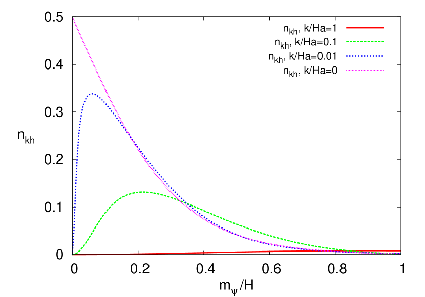
Figure 1: Fermion particle number $n_{\mathbf{k}h}$ as a function of the fermion mass, $m_{\psi}/H$. 4 snapshots are shown, $k/(Ha)=1$ (first Hubble crossing), $k/(Ha)=0.1,0.01,0$ (end of inflation).

In FIG. 1 we show the evolution of the particle number, $n_{\vec{k}h}=n_{\vec{k}h}(m_{\psi}/H)$, during de Sitter inflation. Four snapshots are shown: $k/(Ha)=1,0.1,0.01,0$. Note that most of the particles are created after the first Hubble crossing at $k/a_{1x}=H$. At the end of inflation ($k/(Ha)\simeq 0$) the particle number density approaches the one in Eq. (63).

An interesting question is what happens to the particles produced during inflation in the subsequent epochs of preheating, radiation and matter domination, when we expect the fermionic mass to dissolve. This and related questions are the subject of a forthcoming publication.

V Discussion

As main result of this paper, we have presented the effective fermion mass (37), dynamically generated in de Sitter space. From the thermal features of de Sitter space, and especially from the periodicity of the scalar Green function in imaginary time GibbonsHawking:1977 ; GarbrechtProkopec:2004 , one might expect that additional degrees of freedom coupled to the scalar field thermalise. This would be in analogy with an Unruh detector, which has a thermal response function and, as a consequence of the principle of detailed balance, equilibrates at de Sitter temperature. However, we find no indication of scatterings from a thermal bath or even thermalisation experienced by the fermion through interaction with the scalar field. The apparent reason is, that for an Unruh detector, it is assumed that its internal dynamics is governed by its proper time and that detailed balance holds for the detector GarbrechtProkopec:2004 . One might question whether this requirement may in principle be realised by an experimental device without disturbing the curved background to an extent which spoils the measurement. This is a concern which does not apply to the field theoretical investigation conducted in this work. Nonetheless, the mass generation mechanism fits into the Unruh detector picture when relating it to the Lamb shift of the detector’s energy levels GarbrechtProkopec:2005 , which can also be interpreted as a radiative correction.

Finally, let us discuss in more detail, how the dynamical mass term is related to the familiar Dirac fermion masses. We first note that we can describe the mass generation effect by a nonlocal effective action,

$$S_{\rm eff}=\int d^{4}x\bigg{[}a^{3/2}\bar{\psi}{\rm i}\partial\!\!\!/a^{3/2}\psi-a^{3/2}\bar{\psi}\frac{am_{\psi}^{2}}{{\rm i}\partial\!\!\!/}a^{3/2}\psi\bigg{]}+{\cal O}(s^{0})+S_{\rm anomaly}\,,$$ (66)

where $m_{\psi}$ denotes the fermion mass given in Eq. (37), $1/({\rm i}\partial\!\!\!/)$ is the (retarded) nonlocal operator whose kernel is given in (31) and

$$S_{\rm anomaly}=\int d^{4}x\bigg{[}\frac{f^{2}}{64\pi^{2}}a^{3/2}\bar{\psi}\Big{(}\ln(a){\rm i}\partial\!\!\!/+{\rm i}\partial\!\!\!/\ln(a)\Big{)}a^{3/2}\psi\bigg{]}$$ (67)

is the effective action for the anomaly.

The question is then, what is the difference between the dynamics induced by an ordinary fermion mass term, as implied by the standard action,

$$S_{\rm massive}=\int d^{4}x\Big{[}a^{3/2}\bar{\psi}{\rm i}\partial\!\!\!/a^{3/2}\psi-a^{4}m_{\psi}\bar{\psi}\psi\Big{]}\,,$$ (68)

and the dynamics generated by the nonlocal effective action (66). As we have shown above, these two actions lead to identical second order evolution equations for the chiral densities, $L_{h}$ and $R_{h}$ (and likewise for their linear combinations, $u_{\pm h}$). Yet there is a difference: the nonlocal action (66) conserves chirality, while its local counterpart violates chirality. According to the local action (68), the left and right handed densities evolve according to the first order system (IV), whose graphical representation is shown in terms of mass insertions in FIG. 2. On the other hand, the nonlocal action (66) cannot flip chirality, and its proper graphical representation is shown in FIG. 3. This is the sense in which the fermion mass (37) is not the genuine Dirac mass, which couples left and right handed amplitudes. One may think of the equation of motion for the L-handed (R-handed) fermions as being governed by the system of equations (39), but one should keep in mind that the fermions of opposite chirality are “ghost” fermions and do not comprise physically measurable states. This is to be contrasted with the photons in de Sitter background, which acquire a mass through interactions with a scalar medium, and thus an additional longitudinal physical degree of freedom Prokopec:PhotonMass ; ProkopecPuchwein:2003 .

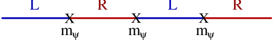
Figure 2: Mass insertions for the local fermion Dirac mass term (68). These insertions violate chirality.

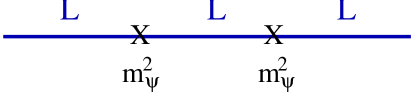
Figure 3: Quadratic fermionic mass insertions corresponding to the nonlocal effective action (66), which preserve chirality.

Putting these findings together suggests dynamical mass generation for interacting quantum fields as a phenomenon generically occuring in de Sitter space. Therefore, it is well conceivable that this mechanism may cause effects during cosmic inflation which lead to observable signatures.

References

• (1) T. Prokopec and R. P. Woodard, “Production of massless fermions during inflation,” JHEP 0310 (2003) 059 [arXiv:astro-ph/0309593]; ibid. Erratum.
• (2) T. Prokopec, “Cosmological magnetic fields from photon coupling to fermions and bosons in inflation,” arXiv:astro-ph/0106247; T. Prokopec, O. Tornkvist and R. P. Woodard, “Photon mass from inflation,” Phys. Rev. Lett.  89 (2002) 101301 [arXiv:astro-ph/0205331];
T. Prokopec, O. Tornkvist and R. P. Woodard, “One loop vacuum polarization in a locally de Sitter background,” Annals Phys.  303 (2003) 251 [arXiv:gr-qc/0205130];
T. Prokopec and R. P. Woodard, “Vacuum polarization and photon mass in inflation,” Am. J. Phys.  72 (2004) 60 [arXiv:astro-ph/0303358];
T. Prokopec and R. P. Woodard, “Dynamics of super-horizon photons during inflation with vacuum polarization,” Annals Phys.  312 (2004) 1 [arXiv:gr-qc/0310056].
T. Prokopec and E. Puchwein, “Nearly minimal magnetogenesis,” Phys. Rev. D 70 (2004) 043004 [arXiv:astro-ph/0403335].
• (3) T. Prokopec and E. Puchwein, “Photon mass generation during inflation: de Sitter invariant case,” JCAP 0404 (2004) 007 [arXiv:astro-ph/0312274].
• (4) S. P. Miao and R. P. Woodard, “The fermion self-energy during inflation,” arXiv:gr-qc/0511140.
• (5) G. W. Gibbons and S. W. Hawking, “Cosmological Event Horizons, Thermodynamics, And Particle Creation,” Phys. Rev. D 15 (1977) 2738.
• (6) B. Garbrecht and T. Prokopec, “Energy density in expanding universes as seen by Unruh’s detector,” Phys. Rev. D 70 (2004) 083529 [arXiv:gr-qc/0406114].
• (7) B. Garbrecht and T. Prokopec, “Lamb shift of Unruh detector levels,” arXiv:gr-qc/0510120.
• (8) N. A. Chernikov and E. A. Tagirov, “Quantum Theory Of Scalar Fields In De Sitter Space-Time,” Annales Poincare Phys. Theor. A 9 (1968) 109.
• (9) N. C. Tsamis and R. P. Woodard, “The Physical basis for infrared divergences in inflationary quantum gravity,” Class. Quant. Grav.  11 (1994) 2969.
• (10) B. Allen, “Vacuum States In De Sitter Space,” Phys. Rev. D 32 (1985) 3136.
• (11) B. Garbrecht, T. Prokopec and M. G. Schmidt, “Particle number in kinetic theory,” Eur. Phys. J. C 38 (2004) 135 [arXiv:hep-th/0211219].
• (12) Izrail Solomonovich Gradshteyn, Iosif Moiseevich Ryzhik, Table of integrals, series, and products, 4th edition, Academic Press, New York (1965).
• (13) B. Garbrecht, “Some aspects of inflationary particle production,” (Ph.D. disertation) http://www.ub.uni-heidelberg.de/archiv/5641
• (14) B. Garbrecht and T. Prokopec, “Unruh response functions for scalar fields in de Sitter space,” Class. Quant. Grav.  21 (2004) 4993 [arXiv:gr-qc/0404058].