Stochastic Background from Coalescences of NS-NS Binaries

Abstract

In this work, numerical simulations were used to investigate the gravitational stochastic background produced by coalescences occurring up to $z\sim 5$ of double neutron star systems. The cosmic coalescence rate was derived from Monte Carlo methods using the probability distributions for forming a massive binary and to occur a coalescence in a given redshift. A truly continuous background is produced by events located only beyond the critical redshift $z_{*}=0.23$. Events occurring in the redshift interval $0.027<z<0.23$ give origin to a “popcorn” noise, while those arising closer than $z=0.027$ produce a shot noise. The gravitational density parameter $\Omega_{gw}$ for the continuous background reaches a maximum around 670 Hz with an amplitude of $1.1\times 10^{-9}$, while the “popcorn” noise has an amplitude about one order of magnitude higher and the maximum occurs around a frequency of 1.2 kHz. The signal is below the sensitivity of the first generation of detectors but could be detectable by the future generation of ground based interferometers. Correlating two coincident advanced-LIGO detectors or two EGO interferometers, the expected S/N ratio are respectively 0.5 and 10.

1 Introduction

The merger of two neutron stars, two black holes or a black hole and a neutron star are among the most important sources of gravitational waves (GW), due to the huge energy released in the process. In particular, the coalescence of double neutron stars (DNS) may radiate about 10⁵³ erg in the last seconds of their inspiral trajectory, at frequencies up to 1.4-1.6 kHz, range covered by most of the ground-based laser interferometers like VIRGO (Bradaschia et al., 1990), LIGO (Abramovici et al., 1992), GEO (Hough, 1992) or TAMA (Kuroda et al., 1997). Besides the amount of energy involved in these events, the rate at which they occur in the local universe is another parameter characterizing if these mergings are or not potential interesting sources of GW. In spite of the large amount of work performed in the past years, uncertainties persist in estimates of the DNS coalescence rate. In a previous investigation, we have revisited this question (de Freitas Pacheco et al., 2005; Regimbau et al., 2005), taking into account the galactic star formation history derived directly from observations and including the contribution of elliptical galaxies when estimating the mean merging rate in the local universe. Based on these results, we have predicted a detection rate of one event every 125 and 148 years by initial LIGO and VIRGO respectively and up to 6 detections per year in their advanced configurations.

Besides the emission produced by the coalescence of the nearest DNS, the superposition of a large number of unresolved sources at high redshifts will produce a stochastic background of GW. In the past years, different astrophysical processes susceptible to generate a stochastic background have been investigated. On the one hand, distorted black holes (Ferrari et al., 1999; de Araujo et al., 2000), bar mode emission from young neutron stars (Regimbau, 2001) are examples of sources able to generate a shot noise (time interval between events large in comparison with duration of a single event), while supernovas or hypernovas (Blair & Ju, 1997; Coward et al., 2001, 2002; Buonanno et al., 2004) are expected to produce an intermediate “popcorn” noise. On the other hand, the contribution of tri-axial rotating neutron stars (Regimbau & de Freitas Pacheco, 2001), including magnetars (Regimbau & de Freitas Pacheco, 2005), constitutes a truly continuous background.

Populations of compact binaries as, for instance, the cataclismic variables are responsible for the existence of a galactic background of GW in the mHz domain, which could represent an important source of confusion noise for space detectors as LISA (Evans et al., 1987; Hils et al., 1990; Bender & Hils, 1997; Postnov & Prokhorov, 1998; Nelenan et al., 2001; Timpano et al., 2005). These investigations have been extended recently to the extra-galactic contribution. Schneider et al. (2001), Kim et al. (2003) and Cooray (2004) considered cosmological populations of double and mixed systems involving black holes, neutron stars and white dwarfs, while close binaries originated from low and intermediate mass stars were discussed by Farmer & Phinney (2002).

In this work, using the DNS merging rate estimated in our precedent study, we have estimated the gravitational wave background spectrum produced by these coalescences. Numerical simulations based on Monte Carlo methods were performed in order to determine the critical redshift $z_{*}$ beyond which the duty cycle condition required to have a continuous background ($D>1$) is satisfied. Unlike previous studies which focus their attention on the early low frequency inspiral phase covered by LISA (Schneider et al., 2001; Farmer & Phinney, 2002; Cooray, 2004), here we are mainly interested in the few thousand seconds before the last stable orbit is reached, when more than 96% of the gravitational wave energy is released. The signal frequency is in the range 10-1500 Hz, covered by ground based interferometers. The paper is organized as follows. In §2, the simulations are described; in §3 the contribution of DNS coalescences to the stochastic background is calculated; in §4 the detection possibility with laser beam interferometers is discussed and, finally, in §5 the main conclusions are summarized.

2 The Simulations

In order to simulate by Monte Carlo methods the occurrence of merging events, we have adopted the following procedure. The first step was to estimate the probability for a given pair of massive stars, supposed to be the progenitors of DNS, be formed at a given redshift. This probability distribution is essentially given by the cosmic star formation rate (Coward et al., 2002), normalized in the redshift interval $0\leq z\leq 5$, e.g.,

$$P_{f}(z)=\frac{dR_{f}(z)/dz}{N_{p}}$$ (1)

The normalization factor in the denominator is essentially the rate at which massive binaries are formed in the considered redshift interval, e.g.,

$$N_{p}=\int_{0}^{5}(dR_{f}(z)/dz)dz,$$ (2)

which depends on the adopted cosmic star formation rate, as we shall see later.

The formation rate of massive binaries per redshift interval is

$$R_{zf}(z_{f})=\frac{dR_{f}(z_{f})}{dz_{f}}=\lambda_{p}\frac{R^{*}_{f}(z_{f})}{1+z_{f}}{\frac{{dV(z_{f})}}{{dz_{f}}}}$$ (3)

In the equation above, $R^{*}_{f}(z)$ is the cosmic star formation rate (SFR) expressed in M_⊙ Mpc^-3yr^-1 and $\lambda_{p}$ is the mass fraction converted into DNS progenitors. Hereafter, rates per comoving volume will always be indicated by the superscript ’*’, while rates with indexes “z_f” or “z_c” refer to differential rates per redshift interval, including all cosmological factors. The (1+z) term in the denominator of eq. 3 corrects the star formation rate by time dilatation due to the cosmic expansion. In the present work we assume that the parameter $\lambda_{p}$ does not change significantly with the redshift and thus it will be considered as a constant. In fact, this term is the product of three other parameters, namely,

$$\lambda_{p}=\beta_{NS}f_{b}\lambda_{NS}$$ (4)

where $\beta_{NS}$ is the fraction of binaries which remains bounded after the second supernova event, $f_{b}$ is the fraction of massive binaries formed among all stars and $\lambda_{NS}$ is the mass fraction of neutron star progenitors.

According to the results by de Freitas Pacheco et al. (2005),Regimbau et al. (2005), $\beta_{NS}$ = 0.024 and $f_{b}$ = 0.136, values which will be adopted in our calculations. Assuming that progenitors with initial masses above 40 M_⊙ will produce black holes and considering an initial mass function (IMF) of the form $\xi(m)=Am^{-\gamma}$, with $\gamma$ = 2.35   (Salpeter’s law), normalized within the mass interval 0.1 - 80 M_⊙ such as $\int m\xi(m)dm$ = 1, it results finally $\lambda_{NS}=\int_{9}^{40}\xi(m)dm=5.72~{}\times 10^{-3}~{}M_{\odot}^{-1}$ and $\lambda_{p}=1.85\times 10^{-5}$ M${}_{\odot}^{-1}$. The evaluation of the parameters $\beta_{NS}$ and $f_{b}$ depends on different assumptions, which explain why estimates of the coalescence rate of DNS found in the literature may vary by one or even two orders of magnitude. The evolutionary scenario of massive binaries considered in our calculations (see de Freitas Pacheco et al. (2005) for details) is similar to that developed by Belczyński et al. (2002), in which none of the stars ever had the chance of being recycled by accretion. Besides the evolutionary path, the resulting fraction $\beta_{NS}$ of bound NS-NS binaries depends on the adopted velocity distribution of the natal kick. The imparted kick may unbind binaries which otherwise might have remained bound or, less probably, conserve bound systems which without the kick would have been disrupted. The adopted value for $\beta_{NS}$ corresponds to a 1-D velocity dispersion of about 80 km/s. This value is smaller than those usually assumed for single pulsars, but consistent with recent analyses of the spin period-eccentricity relation for NS-NS binaries (Dewi et al., 2005). Had we adopted a higher velocity dispersion in our simulations (230 km/s instead of 80 km/s), the resulting fraction of bound systems is reduced by one order of magnitude, e.g., $\beta_{NS}$ = 0.0029. If, on the one hand the fraction of bound NS-NS systems after the second supernova event depends on the previous evolutionary history of the progenitors and on the kick velocity distribution, on the other hand estimates of the fraction $f_{b}$ of massive binaries formed among all stars depends on the ratio between single and double NS systems in the Galaxy and on the value of $\beta_{NS}$ itself (de Freitas Pacheco et al., 2005). We have estimated relative uncertainties of about $\sigma_{f_{b}}/f_{b}\approx 0.5$ and $\sigma_{\beta_{NS}}/\beta_{NS}\approx 0.75$, leading to a relative uncertainty in the parameter $\lambda_{p}$ of about $\sigma_{\lambda_{p}}/\lambda_{p}\approx 0.9$. However, we emphasize that these are only formal uncertainties resulting from our simulations, which depend on the adopted evolutionary scenario for the progenitors. A comparison with other estimates can be found in de Freitas Pacheco et al. (2005).

The element of comoving volume is given by

$$dV(z)=4\pi r(z)^{2}\frac{c}{H_{o}}\frac{dz}{E(\Omega_{i},z)}$$ (5)

with

$$E(\Omega_{i},z)=[\Omega_{m}(1+z)^{3}+\Omega_{v}]^{1/2}$$ (6)

where $\Omega_{m}$ and $\Omega_{v}$ are respectively the present values of the density parameters due to matter (baryonic and non-baryonic) and vacuum, corresponding to a non-zero cosmological constant. A “flat” cosmological model ($\Omega_{m}+\Omega_{v}=1$) was assumed. In our calculations, we have taken $\Omega_{m}$ = 0.30 and $\Omega_{v}$ = 0.70, corresponding to the so-called “concordance” model derived from observations of distant type Ia supernovae (Schmidt et al., 1998) and the power spectra of the cosmic microwave background fluctuations (Spergel, 2003). The Hubble parameter H₀ was taken to be $65\,\mathrm{km\,s}^{-1}\mathrm{Mpc}^{-1}$.

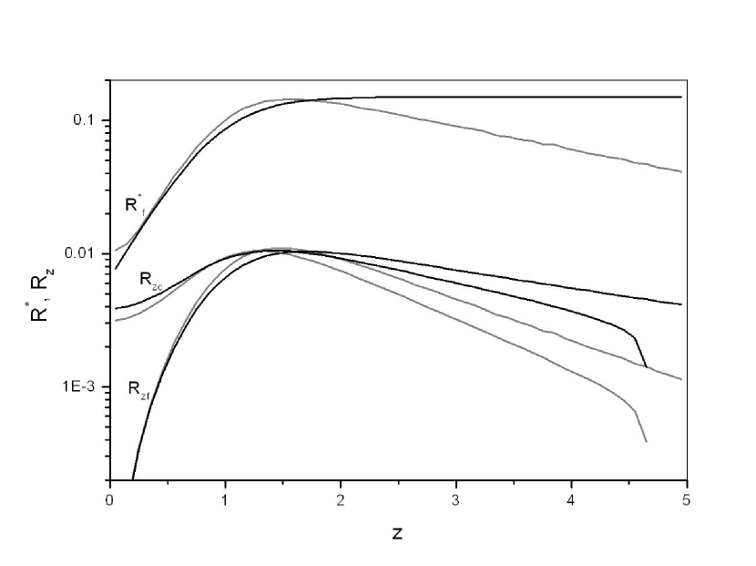
Figure 1: Cosmic star formation rate $R^{*}_{f}(z)$ in M_⊙Mpc^-3yr^-1 in a flat cosmology with $\Omega_{m}$ = 0.30 and $\Omega_{v}$ =0.70: SFR2 is represented by a black line and SFR1 by a grey line. The formation and the coalescence rate per redshift interval are also plotted for comparison.

Porciani & Madau (2001) provide three models for the cosmic SFR history up to redshifts $z\sim 5$. Differences among these models are mainly due to various corrections applied, in particular those due to extinction by the cosmic dust. In our computations, we have considered the second model, labelled SFR2 (Madau et al., 1998) but numerical results using SFR1 (Steidel, 1999) will be also given for comparison. Both rates increase rapidly between $z\sim 0-1$ and peak at $z\sim 1-2$, but SFR1 decreases gently after $z\sim 2$ while SFR2 remains more or less constant (Figure 1).

The next step consists to estimate the redshift $z_{b}$ at which the progenitors have already evolved and the system is now constituted by two neutron stars. This moment fixes also the beginning of the inspiral phase. If $\tau_{b}$ ($\approx 10^{8}$ yr) is the mean lifetime of the progenitors (average weighted by the IMF in the interval 9-40 M_⊙) then

$$z_{b}=z_{f}-H_{0}\tau_{b}(1+z_{f})E(z_{f})$$ (7)

Once the beginning of the inspiral phase is established, the redshift at which the coalescence occurs is estimated by the following procedure. The duration of the inspiral phase depends on the orbital parameters just after the second supernova and on the neutron star masses. The probability for a given DNS system to coalesce in a timescale $\tau$ was initially derived by de Freitas Pacheco (1997), confirmed by subsequent simulations (Vincent, 2002; de Freitas Pacheco et al., 2005) and is given by

$$P_{\tau}(\tau)=B/\tau$$ (8)

Simulations indicate a minimum coalescence timescale $\tau_{0}=2\times 10^{5}$ yr but a considerable number of systems have a coalescence timescale higher than the Hubble time. The normalized probability in the range $2\times 10^{5}$ yr up to 20 Gyr implies $B=0.087$. Therefore, the redshift $z_{c}$ at which the coalescence occurs after a timescale $\tau$ is derived from the equation

$$H_{0}\tau=\int_{z_{c}}^{z_{b}}\frac{dz}{(1+z)E(z)}$$ (9)

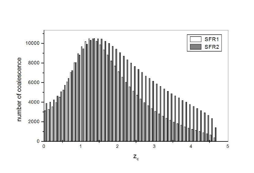
Figure 2: Distribution of coalescences as a function of the redshift derived from our simulations, corresponding to $10^{7}$ numerical experiments.

which was solved in our code by an iterative method. The resulting distribution of the number of coalescences as a function of $z_{c}$ is shown in Figure 2 for both star formation rates SFR1 and SFR2, while the corresponding coalescence rate per redshift interval, $R_{zc}(z)$, is shown in Figure 1. In the same figure, for comparison, we have plotted the formation rate $R_{zf}(z)$ (eq. 3). Notice that the maximum of $R_{zc}(z)$ is shifted towards lower redshifts with respect to the maximum of $R_{zf}(z)$, reflecting the time delay between the formation of the progenitors and the coalescence event. The coalescence rate $R_{zc}(z)$, does not fall to zero at $z=0$ because a non negligible fraction of coalescences ($\sim 3\%$ for SFR2 and $\sim 5\%$ for SFR1) occurs later than $z=0$.

3 The Gravitational Wave Background

The nature of the background is determined by the duty cycle defined as the ratio of the typical duration of a single burst $\bar{\tau}$ to the average time interval between successive events, e.g.,

$$D(z_{*})=\int_{0}^{z_{*}}\bar{\tau}(1+z^{\prime})R_{zc}(z^{\prime})dz^{\prime}$$ (10)

The critical redshift $z_{*}$ at which the background becomes continuous is fixed by the condition $D(z)>1$. Since we are interested in the last instants of the inspiral, when the signal is within the frequency band of ground based interferometers, we took $\bar{\tau}=1000$ s, duration which includes about $96\%$ of the total energy released (see Table 1). From our numerical experiments and imposing D = 1, one obtains $z_{*}=0.23$ when the SFR2 is used and $z_{*}=0.27$ for the SFR1. About 96% (94% in the case of SFR1) of coalescences occur above such a redshift, contributing to the production of a continuous background. Sources in the redshift interval $0.027<z<0.23$ (SFR2) or $0.032<z<0.27$ (SFR1) correspond to a duty cycle D = 0.1 and they are responsible for a cosmic “popcorn” noise.

The gravitational fluence (given here in erg cm^-2Hz^-1) in the observer frame produced by a given DNS coalescence is:

$$f_{\nu_{o}}=\frac{1}{4\pi d_{L}^{2}}\frac{dE_{gw}}{d\nu}(1+z_{c})$$ (11)

where $d_{L}=(1+z_{c})r$ is the distance luminosity, $r$ is the proper distance, which depends on the adopted cosmology, ${dE_{gw}}/{d\nu}$ is the gravitational spectral energy and $\nu=(1+z_{c})\nu_{o}$ the frequency in the source frame. In the quadrupolar approximation and for a binary system with masses $m_{1}$ and $m_{2}$ in a circular orbit:

$$dE_{gw}/{d\nu}=K\nu^{-1/3}$$ (12)

where the fact that the gravitational wave frequency is twice the orbital frequency was taken into account. Then

$$K=\frac{(G\pi)^{2/3}}{3}\frac{m_{1}m_{2}}{(m_{1}+m_{2})^{1/3}}$$ (13)

Assuming $m_{1}=m_{2}=1.4$ one obtains $K=5.2\times 10^{50}$ erg Hz^-2/3.

The spectral properties of the stochastic background are characterized by the dimensionless parameter (Ferrari et al., 1999):

$$\Omega_{gw}(\nu_{o})=\frac{1}{c^{3}\rho_{c}}{\nu_{o}}F_{\nu_{o}}$$ (14)

where $\nu_{o}$ is the wave frequency in the observer frame, $\rho_{c}$ is the critical mass density needed to close the Universe, related to the Hubble parameter $H_{0}$ by,

$$\rho_{c}=\frac{3H_{o}^{2}}{8\pi G}$$ (15)

$F_{\nu_{o}}$ is the gravitational wave flux (given here in erg cm^-2Hz^-1s^-1) at the observer frequency $\nu_{o}$, integrated over all sources at redshifts $z_{c}>z_{*}$, namely

$$F_{\nu_{o}}=\int_{z_{*}}^{z_{\max}}f_{\nu_{o}}dR_{c}(z)$$ (16)

Instead of solving analytically the equation above by introducing, for instance, an adequate fit of the cosmic coalescence rate, we have calculated the integrated gravitational flux by summing individual fluences (eq. 11), scaled by the ratio between the expected number of events per unit of time and the number of simulated coalescences or, in other words, the ratio between the total formation rate of progenitors (eq. 2) and the number of simulated massive binaries, e.g.,

$$F_{\nu_{o}}=\frac{N_{p}}{N_{sim}}\sum_{i=1}^{N_{sim}}f_{\nu_{o}}^{i}$$ (17)

The number of runs (or $N_{sim}$) in our simulations was equal to $10^{7}$, representing an uncertainty of $\leq$ 0.1% in the density parameter $\Omega_{gw}$. Using the SFR2, the derived formation rate of progenitors is $N_{p}=0.031~{}s^{-1}$, whereas for the SFR1 one obtains $N_{p}=0.024~{}s^{-1}$. For each run, the probability distribution $P_{f}(z)$ defines, via Monte Carlo, the redshift at which the massive binary is formed. The beginning of the inspiral phase at $z_{b}$ is fixed by eq. 7. Then, in next step, the probability distribution of the coalescence timescale and eq. 9 define the redshift $z_{c}$ at which the merging occurs. The fluence produced by this event is calculated by eq. 11, stored in different frequency bins in the observer frame and added according to the equation above.

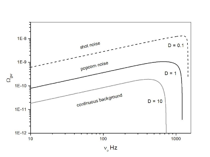
Figure 4: Spectrum of the expected gravitational energy density parameter $\Omega_{gw}$ corresponding to NS-NS coalescences occurring beyond $z_{*}=0.23$ (bold continuous curve). A more conservative background ($D>10$) corresponding to sources beyond $z=1.05$ is plotted for comparison (grey continuous curve). The expected “popcorn” noise contribution arising from sources in the redshift interval $0.027<z<0.23$ (dashed curve) is also shown. This corresponds to the intermediate zone between a shot noise ($D<0.1$) and a continuous background ($D>1$).

Figure  4 shows the density parameter $\Omega_{gw}$ as a function of the observed frequency derived from our simulations. The density parameter $\Omega_{gw}$ increases as $\nu_{o}^{2/3}$ at low frequencies, reaches a maximum amplitude of about $1.1\times 10^{-9}$ around 670 Hz in the case of SFR2 and a maximum of $8.4\times 10^{-10}$) around 630 Hz, in the case of SFR1. A high frequency cut-off at $\sim 1220$ Hz ($\sim 1170$ Hz for SFR1 ) is observed, corresponding approximately to the frequency of the last stable orbit at the critical redshift $z_{*}=0.23$ ($z_{*}=0.27$ for SFR1). Calculations performed by Schneider et al. (2001), in spite of the similar local merging rates, indicate that the maximum occurs at lower frequencies ($\sim$ 100 Hz) with an amplitude (scaled to the Hubble parameter adopted in this work) lower by a factor of seven. However, as those authors have stressed, their calculations are expected to be accurate in the frequency range 10 $\mu$Hz up to 1 Hz, since they have set the value of the maximum frequency $\nu_{max}$ to about that expected at a separation of three times the “last stable orbit” (LSO), e.g., $\nu_{max}\approx 0.19\nu_{LSO}$. Thus, a direct comparison with our results is probably meaningless.

A more conservative estimate can be obtained if one adopts a higher duty cycle value, namely, $D>10$, corresponding to sources located beyond $z\sim 1.05$ ($z\sim 1.075$ for SFR1). Our results are plotted in Fig. 4, which includes, for comparison, the “popcorn” noise contribution arising from sources between $0.027<z<0.23$ ($0.032<z<0.27$ for SFR1), corresponding to the intermediate zone between a shot noise ($D<0.1$) and a continuous background ($D>1$). When increasing the critical redshift (or removing the nearest sources), the amplitude of $\Omega_{gw}$ decreases and the spectrum is shifted toward lower frequencies. The amplitude of the “popcorn” background is about one order of magnitude higher than the continuous background, with a maximum of about $\Omega_{gw}=1.3\times 10^{-8}$ ($8.8\times 10^{-9}$ for SFR1) around a frequency of $1.2$ kHz.

Since some authors use, instead of $\Omega_{gw}$, the gravitational strain $\sqrt{S_{h}}$ defined by Allen & Romano (1999) as

$$S_{h}(\nu_{o})=\frac{3H_{0}^{2}}{10\pi^{2}}\frac{1}{\nu_{o}^{3}}\Omega_{\rm gw}(\nu_{o})$$ (18)

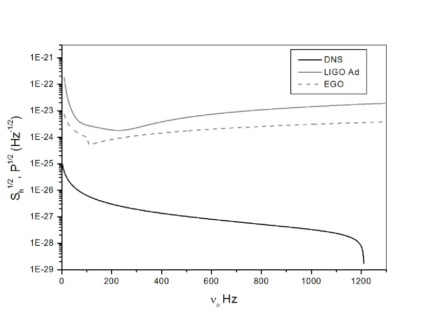
Figure 5: Gravitational strain in Hz^-1/2 corresponding to NS-NS coalescences occurring beyond $z_{*}=0.23$, along with the planned sensitivity curves of LIGO Ad (continuous curve) and EGO (dashed curve).

we show this quantity in Figure 5.

4 Detection

Because the background obeys a Gaussian statistic and can be confounded with the instrumental noise background of a single detector, the optimal detection strategy is to cross-correlate the output of two (or more) detectors, assumed to have independent spectral noises. The cross correlation product is given by (Allen & Romano, 1999):

$$Y=\int_{-\infty}^{\infty}\tilde{s_{1}}^{*}(f)\tilde{Q}(f)\tilde{s_{2}}(f)df$$ (19)

where

$$\tilde{Q}(f)\propto\frac{\Gamma(f)\Omega_{gw}(f)}{f^{3}P_{1}(f)P_{2}(f)}$$ (20)

is a filter that maximizes the signal to noise ratio ($S/R$). In the above equations, $P_{1}(f)$ and $P_{2}(f)$ are the power spectral noise densities of the two detectors and $\Gamma$ is the non-normalized overlap reduction function, characterizing the loss of sensitivity due to the separation and the relative orientation of the detectors. The optimized $S/N$ ratio for an integration time $T$ is given by (Allen, 1997) :

$$(\frac{S}{N})^{2}=\frac{9H_{0}^{4}}{8\pi^{4}}T\int_{0}^{\infty}df\frac{\Gamma^{2}(f)\Omega_{gw}^{2}(f)}{f^{6}P_{1}(f)P_{2}(f)}.$$ (21)

In the literature, the sensitivity of detector pairs is usually given in terms of the minimum detectable amplitude for a flat spectrum ($\Omega_{gw}$ equal to constant) (Allen & Romano, 1999), e.g.,

$$\Omega_{min}=\frac{4\pi^{2}}{3H_{0}^{2}\sqrt{T}}({\rm erfc}^{-1}(2\alpha)-{\rm erfc}^{-1}(2\gamma))[\int_{0}^{\infty}df\frac{\Gamma^{2}(f)}{f^{6}P_{1}(f)P_{2}(f)}]^{-1/2}$$ (22)

The expected minimum detectable amplitude for the main pair of detectors in the world, after one year integration, are given in Table 2, for a detection rate $\alpha=90\%$ and a false alarm rate $\gamma=10\%$. The power spectral densities expressions used for the present calculation can be found in Damour et al. (2001). $\Omega_{min}$ is of the order of $10^{-6}-10^{-5}$ for the first generation of interferometers combined as LIGO/LIGO and LIGO/VIRGO. Their advanced counterparts will permit an increase of two or even three orders of magnitude in sensitivity ($\Omega_{min}\sim 10^{-9}-10^{-8}$). The pair formed by the co-located and co-aligned LIGO Hanford detectors, for which the overlap reduction function is equal to one, is potentially one order of magnitude more sensitive than the Hanford/Livingston pair, provided that instrumental and environmental noises could be removed.

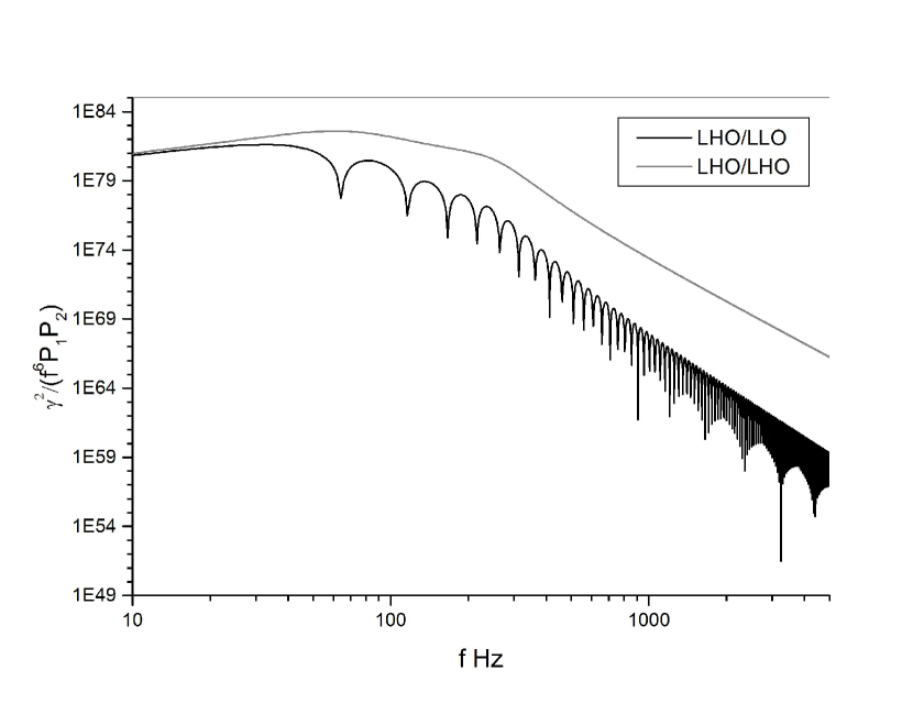
Figure 6: Integrand of the signal-to-noise ratio (eq. 21) for advanced LIGO pairs: LHO-LHO (grey curve) and LHO-LLO (black curve)

However, because the spectrum of DNS coalescences is not flat and the maximum occurs out of the optimal frequency band of ground based interferometers, which is typically around $50-300$ Hz, as shown in Figure 6, the S/N ratio is slightly reduced. Considering the co-located and co-aligned LIGO interferometer pair, we find a signal-to-noise ratio of $S/N\sim 0.002$ ($S/N\sim 0.5$) for the initial (advanced) configuration. Unless the coalescence rate be substantially higher than the present expectations, our results indicate that their contribution to the gravitational background is out of reach of the first and the second generation of interferometers. On the other hand, the sensitivity of the future third generation of detectors, presently in discussion, could be high enough to gain one order of magnitude in the expected S/N ratio. Examples are the Large Scale Cryogenic Gravitational Wave Telescope (LCGT), sponsored by the University of Tokyo and the European antenna EGO (Sathyaprakash, private communication). EGO will incorporate signal recycling, diffractive optics on silicon mirrors, cryo-techniques and kW-class lasers, among other technological improvements. A possible sensitivity for this detector is shown in Figure 5, compared to the expected sensitivity of advanced LIGO. Around 650 Hz, the planned strain noise $\sqrt{S_{n}(\nu)}$ is about $8\times 10^{-24}$ Hz^-1/2 for the advanced LIGO configuration while at this frequency, the planned strain noise for EGO is $2\times 10^{-24}$ Hz^-1/2, which represents a gain by a factor of $\sim 4$. Considering two interferometers located at the same place, we find a signal-to-noise ratio $S/N\sim 10$.

On the other hand, the popcorn noise contribution could be detected by new data analysis techniques currently under investigation, such as the search for anisotropies (Allen & Ottewill, 1997) that can be used to create a map of the GW background (Cornish, 2001), the maximum likelihood statistic (Drasco & Flanagan, 2003), or methods based on the Probability “Event Horizon” concept (Coward & Burman, 2005), which describes the evolution, as a function of the observation time, of the cumulated signal throughout the Universe. The PEH of the GW signal evolves fastly from contributions of high redshift populations, forming a real continuous stochastic background, to low redshift and less probable sources that can be resolved individually, while the PEH of the instrumental noise is expected to evolve much slower. Consequently, the GW signature could be distinguished from the instrumental noise background.

5 Conclusions

In this work, we have performed numerical simulations using Monte Carlo techniques to estimate the occurrence of double neutron star coalescences and the gravitational stochastic background produced these events. Since the coalescence timescale obeys a well defined probability distribution ($P(\tau)\propto 1/\tau$), derived from simulations of the evolution of massive binaries (de Freitas Pacheco et al., 2005), the cosmic coalescence rate does not follow the cosmic star formation rate and presents necessarily a time-lag. In the case where the sources are supernovae or black holes, the gravitational burst is produced in a quite short timescale after the the formation of the progenitors. Therefore, the time-lag is negligible and the comoving volume where the progenitors are formed is practically the same as that where the gravitational wave emission occurs, introducing a considerable simplification in the calculations. This is not the case when NS-NS coalescences are considered, since timescales comparable or even higher than the Hubble timescale have non negligible probabilities. The maximum probability to form a massive binary occurs at $z\sim 1.7$, depending slightly on the adopted cosmic star formation rate, whereas the maximum probability to occur a coalescence is around $z\sim 1.4$.

We have found that a truly continuous background is formed only when sources located beyond $z>0.23$ ($z>0.27$ for the SFR1 case), including 96% (94% for SFR1) of all events and the critical redshift corresponds to the condition $D>1$. Sources in the redshift interval $0.027<z<0.23$ ($0.032<z<0.27$ for SFR1) produce a “popcorn” noise. Our computations indicate that the density parameter $\Omega_{gw}$ has a maximum around 670 Hz (630 Hz for SFR1), attaining an amplitude of about of $1.1\times 10^{-9}$ ($8.3\times 10^{-10}$ for SFR1). The low frequency cutoff around 1.2 kHz corresponds essentially to the gravitational redshifted wave frequency associated to last stable orbit of sources located near the maximum of the coalescence rate.

The computed signal is below the sensitivity of the first and the second generation of detectors. However, using the planned sensitivity of third generation interferometers, we found that after one year of integration, the cross-correlation of two EGO like coincident antennas, gives an the optimized signal-to-noise of $S/R\sim 10$.

The “popcorn” contribution is one order of magnitude higher with a maximum of $\Omega_{gw}\sim 1.3\times 10^{-8}$ ($8.8\times 10^{-9}$ for SFR1) at $\sim 1.2$ kHz. This signal, which is characterized by the spatial and temporal evolution of the events as well as by its signature, can be distinguished from the instrumental noise background and adequate data analysis strategies for its detection are currently under investigation (Allen & Ottewill, 1997; Cornish, 2001; Drasco & Flanagan, 2003; Coward & Burman, 2005).

Acknowledgement

The authors thanks the referee by his useful comments, which have improved the early version of this paper.

Table 1: For three values of the emission frequency (column 1), the corresponding time left to the last stable orbit (second column) and percentage of energy released (third column)

$\nu_{min}$ (Hz)	$\bar{\tau}$	$\Delta E/E_{T}$ ($\%$)
100	2 s	84
10	1000 s	96
1	5.26 d	99

Table 2: Expected $\Omega_{min}$ of different interferometer pairs for a flat background spectrum and an integration time T = 1 year, a detection rate $\alpha=90\%$ and a false alarm rate $\gamma=10\%$. LHO and LLO stand for LIGO Hanford Observatory and LIGO Livingston Observatory

	LHO-LHO	LHO-LLO	LLO-VIRGO	VIRGO-GEO
initial	$4\times 10^{-7}$	$4\times 10^{-6}$	$8\times 10^{-6}$	$8\times 10^{-6}$
advanced	$6\times 10^{-9}$	$1\times 10^{-9}$

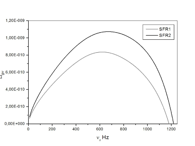
Figure 3: Spectrum of the expected gravitational energy density parameter $\Omega_{gw}$ for the continuous regime. Results are shown for the two star formation rates adopted in this work.

References

- Abramovici et al. (1992) Abramovici A. et al. 1992, Science, 256, 325
- Allen (1997) Allen B. 1997, in Proc. of Relativistic Gravitation and Gravitational Radiation, ed. Marck J. A. and Lasota J. P. (Cambridge:University Press), 373
- Allen & Ottewill (1997) Allen B. and Ottewill A.C. 1997, Phys. Rev. D, 56, 545
- Allen & Romano (1999) Allen B. and Romano J.D. 1999, Phys. Rev. D, 59, 10
- de Araujo et al. (2000) de Araujo J.C.N., Miranda O.D. and Aguiar O.D. 2000, Nu.Ph.S., 80, 7
- Belczyński et al. (2002) Belczyński K., Kalogera V. and Bulik T. 2002, ApJ, 572, 407
- Bender & Hils (1997) Bender P.L and Hils D. 1997, Class. Quant. Grav., 14, 1439
- Blair & Ju (1997) Blair D. and Ju L., 1996, MNRAS, 283, 648
- Bradaschia et al. (1990) Bradaschia C. et al. 1990, Nucl. Instrum. Meth., A289, 518
- Buonanno et al. (2004) Buonanno A., Sigl G., Janka H. T. and Mueller E. 2005, Phys. Rev. D, 72, 8
- Cooray (2004) Cooray A. 2004, MNRAS, 354, 25
- Cornish (2001) Cornish N.J. 2001, Class. Quant. Grav., 18, 4277
- Coward & Burman (2005) Coward D. and Burman R.R. 2005, MNRAS, 361, 362
- Coward et al. (2001) Coward D., Burman R.R. and Blair D. 2001, MNRAS, 324, 1015
- Coward et al. (2002) Coward D., Burman R.R. and Blair D. 2001, MNRAS, 329, 411
- Damour et al. (2001) Damour T., Iyer B.R. and Sathyaprakash B.S. 2001, Phys. Rev. D, 63, 4
- Drasco & Flanagan (2003) Drasco S. and Flanagan E.E. 2003, Phys. Rev. D, 67, 8
- Evans et al. (1987) Evans C.R., Iben I. and Smarr L. 1987, ApJ, 323, 129
- de Freitas Pacheco (1997) de Freitas Pacheco, J.A., 1997, Astrop. Phys., 8, 21
- de Freitas Pacheco et al. (2005) de Freitas Pacheco J.A., Regimbau T., Spallici A. and Vincent S. 2005, IJMPD, in press; astro-ph/0510727
- Dewi et al. (2005) Dewi J.D.M., Podsiadlowski Ph. and Pols O.R., 2005, MNRAS, in press; astr-ph/0507638
- Farmer & Phinney (2002) Farmer A.J. and Phinney E.S. 2002, AAS, 34, 1225
- Hils et al. (1990) Hils D., Bender P.L and Webbink R.F. 1990, ApJ, 360, 75
- Hough (1992) Hough J. 1992, in Proc. of the Sixth Marcel Grossmann Meeting, ed. H. Sato and T. Nakamura, (Singapore: World Scientific), 192
- Kalogera et al. (2001) Kalogera V., Narayan R., Spergel D. N. and Taylor J. H. 2001, ApJ, 556, 340
- Kalogera et al. (2002) V. Kalogera et al., ApJ 601, L179 (2002).
- Kalogera et al. (2004) Kalogera V. et al. 2004, ApJ, 614, L137
- Kim et al. (2003) Kim C., Kalogera V. and Lorimer D. R. 2003, ApJ, 584, 985
- Kim et al. (2003) Kim C., Kalogera V., Lorimer D. R. and White S., 2003, ApJ, 616, 1109
- Kuroda et al. (1997) Kuroda K. et al. 1997, in Proc. of the International Conference on Gravitational Waves: Sources and Detectors, ed. I. Ciufolini & F. Fidecaro, (Singapore: World Scientific), 1007
- Lipunov et al. (1977) Lipunov V.M., Postnov K.A. and Prokhorov M.E., MNRAS, 1997, 288, 245
- Ferrari et al. (1999) Ferrari V., Matarrese S. and Schneider R. 1999, MNRAS, 303, 258
- Madau et al. (1998) Madau P., Pozzetti L., Dickinson A., 1998, ApJ, 498, 106
- Nelenan et al. (2001) Neleman G., Yungelson L. and Potergies Zwart S.F. 2001, A&A, 375, 890
- Phinney (1991) Phinney E. S. 1991, ApJ, 380, L17
- Porciani & Madau (2001) Porciani C. and Madau P. 2001, ApJ, 548, 522
- Postnov & Prokhorov (1998) Postnov K.A. and Prokhorov M.E 1998, ApJ, 494, 674
- Potergies Zwart & Spreeuw (1996) Potergies Zwart S. F. and Spreeuw H. N. 1996, A&A, 312, 670
- Potergies Zwart & Yungelson (1998) Potergies Zwart S. F. and Yungelson L. 1998, A&A, 332, 173
- Regimbau (2001) Regimbau T. 2001, PhD dissertation, University of Nice-Sophia Antipolis, France
- Regimbau & de Freitas Pacheco (2001) Regimbau T. and de Freitas Pacheco J. A. 2001, A&A, 376, 381
- Regimbau & de Freitas Pacheco (2005) Regimbau T. and de Freitas Pacheco J. A. 2005, A&A, in press
- Regimbau et al. (2005) Regimbau T., de Freitas Pacheco J.A., Spallici A. and Vincent S. 2005, CQG, 22, S935
- Schmidt et al. (1998) Schmidt B. et al. 1998, ApJ, 507, 46
- Schneider et al. (2001) Schneider R., Ferrari V., Matarrese S. and Potergies Zwart S.F. 2001, MNRAS, 324, 797
- Spergel (2003) Spergel D.N. et al. 2003, ApJS, 148, 175
- Steidel (1999) Steidel C.C, Adelberger K.L., Giavalisco M., Dickinson M. and Pettini M. 1999, ApJ, 519,1
- Timpano et al. (2005) Timpano S.E, Rubbo L.J. and Cornish N.J. 2005, preprint (gr-qc/0504071)
- Tutukov and Yungelson (1993) Tutukov A.V. and Yungelson L.R. 1993, MNRAS, 260, 675
- van den Heuvel & Lorimer (1996) van den Heuvel E. P. J. and Lorimer D. 1996, MNRAS, 283, L37
- Vincent (2002) Vincent S. 2002, DEA Dissertation, University of Nice-Sophia Antipolis, France