Scaling Laws for the Cosmological Constant

Abstract

We study the expansion of the universe at late times in the case that the cosmological constant obeys certain scaling laws motivated by renormalisation group running in quantum theories. The renormalisation scale is identified with the Hubble scale and the inverse radii of the event and particle horizon, respectively. We find de Sitter solutions, power-law expansion and super-exponential expansion in addition to future singularities of the Big Rip and Big Crunch type.

1 Introduction

The recently observed [1, 2, 3, 4, 5, 6] accelerated expansion of the universe has opened new ways to think about the connection between cosmology and quantum physics since an entire classical origin for the acceleration seems improbable. Quantum theories, on the other hand, potentially yield a lot of sources for dark energy (DE), the energy form that is responsible for the cosmic acceleration [7, 8, 9]. One of the most prominent candidates for DE is a positive cosmological constant (CC) because it appears already in Einstein’s equations of classical general relativity. In this context, it can be treated as a perfect fluid with a constant energy density $\Lambda>0$ and an equation of state (EOS) $\omega=p/\Lambda=-1$ that corresponds to a negative pressure $p=-\Lambda$. Furthermore, on the quantum level the CC can be interpreted as vacuum energy, however, its absolute value has not been predicted reliably in any theory yet, and naive estimates are far too large [10].

In this work we investigate the late-time cosmological evolution in a special class of cosmologies that are based on general relativity with a time-dependent CC and Newton’s constant. Classically both constants are truly time-independent, but quantum effects may induce a scale-dependence in the form of renormalisation group equations (RGE) for these constants. For instance, quantum field theory (QFT) on curved space-times [11, 12] and quantum gravity [13, 14, 15] provide a framework for the renormalisation group running. However, the corresponding RGEs are not unique and the identification of the renormalisation scale $\mu$, on which they depend, is not fixed by the theories. For phenomenological reasons, we should request that the scale $\mu$ does not change too much over cosmological time scales. In contrast to DE scenarios with a time-dependent EOS [16, 17], here, the EOS of the CC is still exactly $\omega=-1$. However, one obtains an effective time-dependent EOS [18] due to the non-standard scaling of the matter energy density with the cosmological time.

The paper is organised as follows: in Sec. 2 we describe three scaling laws for the CC. Two of them are based on QFT on curved space-times, whereas the third one appears in the context of quantum Einstein gravity (QEG) at late cosmological times. In the latter case we also consider the running of Newton’s constant. The identification of the renormalisation scale $\mu$ with some cosmologically relevant quantity is done in Sec. 3. We consider three possible choices for $\mu$: the Hubble scale $H$, the (inverse) radius $R$ of the cosmological event horizon and finally the (inverse) radius $T$ of the particle horizon. In Sec. 4 we discuss how to solve Einstein’s equations on a Robertson-Walker background when the CC and Newton’s constant depend on the cosmological time. The main part of this work can be found in Sec. 5, where we investigate the late-time evolution of the universe for all combinations of scaling laws and scale choices. Since it is not always possible to obtain exact or approximate solutions, some of the given results are numerical. Finally, we present our conclusions in Sec. 6.

2 Scaling laws

According to QFT on curved space-times [11, 12] the CC and Newton’s constant are subject to renormalisation group running like the running of the fine-structure constant in quantum electrodynamics. The RGE for the CC, corresponding to the vacuum energy density $\Lambda$, depends crucially on the considered quantum fields and their masses. For this kind of running we neglect the scale-dependence of Newton’s constant in this work.

In the following we discuss two different RGEs, the first one follows directly from the 1-loop effective action and is given by $\mu\frac{\text{d}\Lambda}{\text{d}\mu}=A_{0}$ in the $\overline{\text{MS}}$-scheme, where quantum fields with masses $M$ determine the coefficient $A_{0}\sim\mp M^{4}$. Note that the sign of $A_{0}$ depends on the spins of the fields, see, e.g., Ref. [19] for the exact expression. Upon integration one obtains in the case of constant masses

$$\frac{\Lambda(\mu)}{\Lambda_{0}}=1-q_{1}\ln\frac{\mu}{\mu_{0}},\,\,\,\,q_{1}\sim\mp\frac{M^{4}}{\Lambda_{0}},$$ (1)

where $\Lambda_{0}$ denotes the vacuum energy density today, when the renormalisation scale $\mu$ has the value $\mu_{0}$. The scaling law (1) has a big disadvantage since it has been derived in a renormalisation scheme that is usually associated with the high-energy regime [20]. It is therefore not known to what extend it can be applied at late times in cosmology. In addition, to avoid conflicts with observations, the field content has to be fine-tuned to obtain $|q_{1}|\leq O(1)$, which we assume for the rest of this work.

The second scaling law follows from a RGE that shows a decoupling behaviour. Considering only the most dominant terms at low energy, the corresponding $\beta$-function for $\Lambda$ is given by $\mu\frac{\text{d}\Lambda}{\text{d}\mu}=A_{1}\mu^{2}$, where $A_{1}\sim\pm M^{2}$ is set by the masses $M$ and the spins of the fields. RGEs of this kind have been studied extensively in the literature [12]. Assuming constant masses and $\mu_{0}$ to be of the order of today’s Hubble scale $H_{0}$ one obtains

$$\frac{\Lambda(\mu)}{\Lambda_{0}}=L_{0}+L_{1}\frac{\mu^{2}}{\mu_{0}^{2}},\,\,\,\,L_{1}\sim\pm\frac{M^{2}}{M_{\text{P}}^{2}},$$ (2)

where $L_{0}:=1-L_{1}$ and $M_{\text{P}}$ denotes the Planck mass today. Here, the running of $\Lambda$ is suppressed since $|L_{1}|\ll 1$ for sub-Planckian masses $M$.

The last scaling laws come from the RGEs in QEG [13, 14]. In this framework the effective gravitational action becomes dependent on a renormalisation scale $\mu$, which leads to RGEs for $\Lambda$ and $G$. An interesting feature is the occurrence of an ultraviolet (UV) fixed-point [21] in the renormalisation group flow of the dimensionless quantities $\Lambda\mu^{-4}$ and $G\mu^{2}$ at very early times in cosmology corresponding to $\mu\rightarrow\infty$. Motivated by strong infrared (IR) effects in quantum gravity one has proposed that there might also exist an infrared fixed-point in QEG [22] leading to significant changes in cosmology at late times, where $\mu\rightarrow 0$. If this were true, one would obtain the RGEs

$$\frac{\Lambda}{\Lambda_{0}}=\frac{\mu^{4}}{\mu_{0}^{4}},\,\,\,\,\frac{G}{G_{0}}=\frac{\mu_{0}^{2}}{\mu^{2}},$$ (3)

where $\mu_{0}$ corresponds to $\Lambda=\Lambda_{0}$ and $G=G_{0}$. In the epoch between the UV and IR fixed-points, $\Lambda$ and $G$ vary very slowly with $\mu$, and we will treat them as constants in this region. Therefore, we assume that the scaling laws (3) are valid from today until the end of the universe.

3 Choice of the scale

In order to study the effects on the cosmological expansion due to the scaling laws of Sec. 2, we have to define the physical meaning of the renormalisation scale $\mu$. Unfortunately, the theories underlying the scaling laws do not determine the scale explicitly, apart from the usual interpretations as an (IR) cutoff or a scale characterising the physical environment (temperature, external momenta). In our cosmological setting we will investigate three different choices for $\mu$, given by the Hubble scale $H$, the inverse radius $R^{-1}$ of the cosmological event horizon, and finally the inverse radius $T^{-1}$ of the particle horizon.

For the purposes of this work we consider a spatially flat Robertson-Walker metric given by the line element

$$\text{d}s^{2}=\text{d}t^{2}-a^{2}(t)\text{d}\vec{x}^{2},$$ (4)

where the scale factor $a(t)$ depends only on the cosmological time $t$ and not on the spatial coordinates $\vec{x}$. While the Hubble scale

$$H(t):=\frac{\dot{a}(t)}{a(t)}$$ (5)

describes the actual expansion rate of the universe, the horizon scales $R$ and $T$ describe the cosmological evolution of the future and the past, respectively. The radius $R$ of the cosmological event horizon corresponds to the proper distance that a (light) signal can travel when it is emitted by a comoving observer at the time $t$:

$$R(t):=a(t)\int_{t}^{\infty}\frac{\text{d}t^{\prime}}{a(t^{\prime})}.$$ (6)

In the case that the universe comes to an end within finite time the upper limit of the integral has to be replaced by this time. Similar to the event horizon of a black hole, the cosmological event horizon exhibits thermodynamical properties like the emission of radiation with the Gibbons-Hawking temperature [25]. The analogue to $R$ is the particle horizon radius $T$, which is given by the proper distance that a signal has travelled since the beginning of the world ($t=0$):

$$T(t):=a(t)\int_{0}^{t}\frac{\text{d}t^{\prime}}{a(t^{\prime})}.$$ (7)

In a simple cosmological model, where the universe begins at $t=0$ and then evolves according to the scale factor $a(t)\propto t^{n}$ with $0<n<1$, the particle horizon radius reads $T(t)=t/(1-n)$. Now we assume that at some time $t_{0}$ a de Sitter phase sets in, which corresponds to a scale factor $a(t)\propto\exp(H_{0}(t-t_{0}))$ for $t>t_{0}$. This leads to a radius function $T$ that grows exponentially with $t$ at late times:

$$T(t>t_{0})=\left(T(t_{0})+\frac{1}{H_{0}}\right)\exp(H_{0}(t-t_{0}))-\frac{1}{H_{0}}.$$ (8)

Since the asymptotic behaviour of the scales $H$, $R$ and $T$ plays a major role in this work, it is plotted in Fig. 1 for a universe with dust-like matter and $\Lambda$ and $G$ being positive and constant.

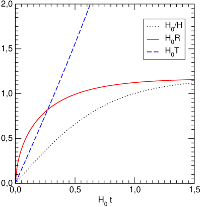
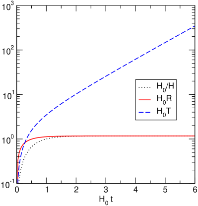
Figure 1: In a spatially flat $\Lambda$CDM universe with constant $\Lambda$ and $G$ the radii of the event horizon $R$ and the Hubble horizon $H^{-1}$ approach the same constant value for $t\rightarrow\infty$. At early times the particle horizon radius $T$ grows linearly with time and exponentially with time for $t\rightarrow\infty$. At the time $t_{0}=0,99H_{0}^{-1}$ (today) the relative vacuum energy is given by $\Omega_{\Lambda 0}=0,73$.

Note that if one of the horizon radii diverges, one says that the horizon does not exist. The geometric meaning of the scales given here has been discussed, e.g., in Ref. [26], and some applications in the context of DE can be found in Refs. [27].

4 Time-dependent $\boldsymbol{\Lambda}$ and $\boldsymbol{G}$

Applying the scaling laws of Sec. 2 together with the identification of the scale $\mu$ with one of the cosmological scales of Sec. 3, we obtain time-dependent functions $\Lambda(t)$ and $G(t)$. Einstein’s equations $G^{\alpha\beta}=8\pi G(\Lambda g^{\alpha\beta}+T^{\alpha\beta})$ and the Einstein tensor $G^{\alpha\beta}$ remain unmodified apart from the additional time-dependence in $\Lambda$ and $G$. For the late-time epoch we consider the spatially flat metric $g^{\alpha\beta}$ following from Eq. (4), and the energy-momentum tensor $T^{\alpha\beta}$ describes a perfect fluid with energy density $\rho$ and pressure $p$. Additionally, we introduce the variable $Q:=(1+3\omega)/2$ which is fixed by the EOS $\omega=p/\rho$ of the fluid. Finally, the evolution of the scale factor $a(t)$ is given by Friedmann’s equations

$$\frac{\dot{a}^{2}}{a^{2}}=\frac{8\pi}{3}G(\Lambda+\rho),\,\,\,\,\frac{\ddot{a}}{a}=\frac{8\pi}{3}G(\Lambda-Q\rho),$$ (9)

which have to agree with the Bianchi identities

$$0=G_{\,\,\,\,\,\,;\beta}^{\alpha\beta}=[G\Lambda g^{\alpha\beta}+GT^{\alpha\beta}]_{;\beta},$$

that imply

$$\dot{G}(\Lambda+\rho)+G(\dot{\Lambda}+\dot{\rho}+2H(Q+1)\rho)=0.$$

For constant $\Lambda$ and $G$ the last equation can be integrated to yield the usual scaling law for the matter energy density $\rho\propto a^{-2(Q+1)}$. In general, this is not possible when $\Lambda$ and $G$ depend on time due to the energy transfer between $\Lambda$ and $\rho$. It therefore implies an effective interaction between the gravitational sector and matter, which is not part of the original Lagrangian. In this sense it should be compared with gravitational particle production [28] resulting also from the interplay of gravity with quantum physics.

To determine the scale factor $a(t)$ we combine both Friedmann’s equations (9) resulting in

$$K_{0}F(t)=\frac{G(t)}{G_{0}}\frac{\Lambda(t)}{\Lambda_{0}}\,\,\,\,\text{with}\,\,\,\,F(t):=\frac{\ddot{a}}{a}+Q\left(\frac{\dot{a}}{a}\right)^{\!2}=\dot{H}+(Q+1)H^{2},$$ (10)

where the constant $K_{0}:=[\Omega_{\Lambda 0}(Q+1)H_{0}^{2}]^{-1}$ is fixed by today’s values of the Hubble scale $H_{0}$, the relative vacuum energy density $\Omega_{\Lambda 0}$ and the matter EOS $Q$.

5 Late-time evolution

In this section we study the late-time evolution of the universe with variable $\Lambda$ and $G$, thereby assuming from today on the validity of the scaling laws (1)–(3) and the correct identification of the renormalisation scale $\mu$ with the scales (5)–(7). Our aim is to determine in all nine cases the possible final states of the universe. This depends, of course, on the choice of parameters, but we restrict ourselves to parameter values which comply vaguely to current observations. Today, at the cosmological time $t_{0}=0,99H_{0}^{-1}$ we fix the initial values $H_{0}$ and $\Omega_{\Lambda 0}=0,73$ by observations. Furthermore, the initial value $T_{0}$ of the particle horizon radius would be fixed if the past cosmological evolution was known from the Big Bang on. In contrast to this, the value $R_{0}$ of today’s event horizon radius depends on the future cosmological evolution and is treated here as a free parameter. In the following we derive some properties of the solutions analytically, in particular, we study the stability of (asymptotic) de Sitter solutions and the occurrence of future singularities [29], where the scale factor or one of its derivatives diverge within finite time. For simplicity we denote a Big Rip or a Big Crunch by the lowest order divergent derivative that is positive or negative, respectively. Since some combinations of scaling laws and renormalisation scales lead to complicated equations we derive in some cases only approximate or numerical statements.

In order to solve Eq. (10) numerically, we have to remove the integrals in the definitions (6), (7) of $R$ and $T$ by a differentiation with respect to $t$. Using the relations

$$\dot{R}=RH-1,\,\,\,\,\dot{T}=TH+1$$

an ordinary differential equation for the scale factor can be obtained and numerically integrated. Afterwards we have to check whether the functions $R$ and $T$, calculated from the numerical solution of $a(t)$, agree with $R$ and $T$ that follow directly from Eq. (10). If they do not match, the numerical solution has to be discarded. Furthermore, solutions involving a negative matter energy density are questionable on physical grounds. This happens when the vacuum energy density $\Lambda$ becomes greater than the critical energy density $\rho_{\text{c}}=3H^{2}/(8\pi G)$, which follows from the first Friedmann equation (9).

5.1 $\boldsymbol{\Lambda=\Lambda_{0}(1-q_{1}\ln\frac{\mu}{\mu_{0}})}$, $\boldsymbol{\mu=H}$

For the given scaling law and scale choice Eq. (10) reads

$$K_{0}(\dot{H}+(Q+1)H^{2})=1-q_{1}\ln\frac{H}{H_{0}}.$$ (11)

We first look for asymptotic de Sitter solutions by applying $\dot{H}=0$ and $H\rightarrow H_{\text{e}}$. Thus the final Hubble scale $H_{\text{e}}$ is given by

$$\frac{H_{\text{e}}^{2}}{H_{0}^{2}}=\frac{q_{1}}{2}\Omega_{\Lambda 0}W_{u}\left(\frac{2}{q_{1}\Omega_{\Lambda 0}}e^{2/q_{1}}\right)\!\!.$$ (12)

Here, $W_{u}(z)$ with $u=0,-1$ denotes one of the two real-valued branches of Lambert’s W-function, which is the solution of $z=xe^{x}$, see Fig. 2.

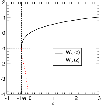
Figure 2: Lambert’s $W$-function is the inverse function of $z=xe^{x}$. For $-1/e\leq z<0$ it has two real-valued brunches $W_{0}(z)$ and $W_{-1}(z)$, and for $z\geq 0$ only $W_{0}(z)$ is real.

For $q_{1}>0$ there is always one solution for $H_{\text{e}}$, and for $q_{1}<0$ two solutions exist if the argument of $W_{u}$ in Eq. (12) is greater than $-e^{-1}$. This means either $q_{1}<n_{1}$ or $q_{1}>n_{2}$ with $n_{1}:=2/W_{0}(-\Omega_{\Lambda 0}e^{-1})$ and $n_{2}:=2/W_{-1}(-\Omega_{\Lambda 0}e^{-1})>n_{1}$. These solution are stable if

$$\left.\frac{\text{d}(K_{0}\dot{H})}{\text{d}H}\right|_{H\rightarrow H_{\text{e}}}=-\frac{q_{1}}{H_{\text{e}}}-2H_{\text{e}}K_{0}(Q+1)<0,$$

where we used Eq. (11). For positive $q_{1}$ this condition is always fulfilled, whereas for negative $q_{1}$ it means $W_{u}(\frac{2}{q_{1}\Omega_{\Lambda 0}}e^{2/q_{1}})<-1$, which follows from Eq. (12). Again, the argument of $W_{u}$ is constrained yielding $q_{1}>n_{2}$. Therefore only $q_{1}>n_{2}$, which includes $q_{1}>0$, leads to stable de Sitter solutions. Using the phase space relation (11), which is plotted in Fig. 3, we conclude that for other values of $q_{1}$ the cosmological evolution will always end within finite time in a Big Crunch singularity, where $H\rightarrow 0$ and $\dot{H}\rightarrow-\infty$.

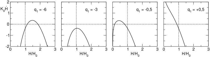
Figure 3: The phase space relation (11) is shown for $q_{1}=-6;-3$, where the universe ends in a Big Crunch singularity, and respectively for $q_{1}=-\frac{1}{2};+\frac{1}{2}$, which leads to a de Sitter final state ($\dot{H}=0$). In all cases the evolution begins at $H=H_{0}$, where $\Omega_{\Lambda 0}=0,73$ and $\dot{H}_{0}<0$.

5.2 $\boldsymbol{\Lambda=\Lambda_{0}(L_{0}+L_{1}\frac{\mu^{2}}{\mu_{0}^{2}})}$, $\boldsymbol{\mu=H}$

Using this choice for $\Lambda$ and $\mu$ Eq. (10) becomes

$$\frac{\ddot{a}}{a}+H^{2}(Q-L_{1}(Q+1)\Omega_{\Lambda 0})=H_{0}^{2}L_{0}\Omega_{\Lambda 0}(Q+1),$$

which has the exact solution

$$\frac{a(t)}{a_{0}}=\left[\sinh([Q+1][\Omega_{\Lambda 0}L_{0}(1-L_{1}\Omega_{\Lambda 0})]^{\frac{1}{2}}H_{0}t)\right]^{n}$$

with

$$n:=[(Q+1)(1-L_{1}\Omega_{\Lambda 0})]^{-1}.$$

At early times, $H_{0}t\ll 1$, it describes a power-law expansion $a(t)\propto t^{n}$, whereas at late times it approaches the de Sitter expansion law $a(t)\propto\exp(H_{\text{e}}t)$ with the final Hubble scale $H_{\text{e}}$ given by

$$H_{\text{e}}=H_{0}\sqrt{\frac{\Omega_{\Lambda 0}L_{0}}{1-L_{1}\Omega_{\Lambda 0}}}.$$

Further aspects of this case have been studied, e.g., in Refs. [12].

5.3 $\boldsymbol{\Lambda G=\Lambda_{0}G_{0}\frac{\mu^{2}}{\mu_{0}^{2}}}$, $\boldsymbol{\mu=H}$

Following Sec. 2 we assume that this scaling law is valid from today on. Here, Eq. (10) is given by $\frac{\ddot{a}}{a}+BH^{2}=0$ with $B:=Q-(Q+1)\Omega_{\Lambda 0}$. It has an exact power-law solution

$$\frac{a(t)}{a_{0}}=[(1+B)(t-t_{1})]^{1/(B+1)},\,\,\,\,t_{1}=\text{const.},$$

that exhibits a constant acceleration $\ddot{a}a/\dot{a}^{2}=-B>0$ as well as $\Omega_{\Lambda}=\text{const}$. A similar solution was found in Refs. [22].

5.4 $\boldsymbol{\Lambda=\Lambda_{0}(1-q_{1}\ln\frac{\mu}{\mu_{0}})}$, $\boldsymbol{\mu=R^{-1}}$

Since this case has been discussed explicitly in Ref. [19], we skip some details in the following discussion. At first we look for de Sitter solutions, where the inverse Hubble scale and the event horizon radius approach $R\rightarrow R_{\text{e}}=H_{\text{e}}^{-1}$ in addition to $\dot{H}=0$. Then $K_{0}F=1+q_{1}\ln\frac{R}{R_{0}}$ can be solved for $R_{\text{e}}$ yielding

$$R_{\text{e}}^{2}=\frac{2}{H_{0}^{2}q_{1}\Omega_{\Lambda 0}W_{u}(\frac{2}{R_{0}^{2}H_{0}^{2}q_{1}\Omega_{\Lambda 0}}e^{2/q_{1}})}.$$ (13)

For positive $q_{1}$ there is always a solution for $R_{\text{e}}$, but it is unstable as can be seen from the following consideration. We first insert $R=R_{0}\exp([K_{0}F-1]/q_{1})$ and $H=\sqrt{K_{0}F/[K_{0}(Q+1)]}$, which is valid in the de Sitter limit, into $K_{0}\dot{F}=q_{1}(H-R^{-1})$. Then we compute

$$\left.\frac{\text{d}(K_{0}\dot{F})}{\text{d}(K_{0}F)}\right|_{\text{dS}}=\frac{q_{1}}{2}[K_{0}^{2}F(Q+1)]^{-\frac{1}{2}}+\frac{1}{R_{0}}\exp\left[\frac{1-K_{0}F}{q_{1}}\right]\!\!,$$ (14)

which is positive for $q_{1}>0$ signalling instability. Thus a Big Crunch singularity ($F,\dot{H}\rightarrow-\infty$, $R\rightarrow 0$) might happen for certain values of initial conditions and parameters, or there exists no solution. A Big Rip singularity ($F,\dot{H}\rightarrow\infty$, $R\rightarrow 0$) does not exist because it is not compatible with $R\rightarrow\infty$.

For negative $q_{1}$ there are two solutions for $R_{\text{e}}$ if the argument of $W_{u}$ in Eq. (13) is greater than $-e^{-1}$ corresponding to the condition

$$R_{0}>\sqrt{\frac{2\exp(2/q_{1}+1)}{-q_{1}H_{0}^{2}\Omega_{\Lambda 0}}}.$$

According to Eq. (14) it turns out that $R_{\text{e}1}:=R_{\text{e}}|_{u=0}$ represents a stable solution and $R_{\text{e}2}:=R_{\text{e}}|_{u=-1}$ an unstable one, respectively. A closer inspection of the solutions $R_{\text{e}1/2}$ shows that $R_{\text{e}1}>R_{0}>R_{\text{e}2}$ if $R_{0}^{2}H_{0}^{2}\Omega_{\Lambda 0}>1$. In the case $R_{0}^{2}H_{0}^{2}\Omega_{\Lambda 0}<1$ the parameter range

$$q_{1}<\frac{2}{W_{0}(-1/(e^{1}q_{3}))}$$

results to $R_{0}>R_{\text{e}1}>R_{\text{e}2}$, whereas

$$q_{1}>\frac{2}{W_{0}(-1/(e^{1}q_{3}))}$$

leads to $R_{\text{e}1}>R_{\text{e}2}>R_{0}$, respectively. Moreover, all stable de Sitter solutions are realised except the last one corresponding to the parameter region ($R_{0}^{2}H_{0}^{2}\Omega_{\Lambda 0}<1$, $q_{1}>2/W_{0}[-1/(e^{1}q_{3})]$). In this last case the universe will end in a Big Rip singularity, where $F,\dot{H}\rightarrow\infty$ and $R\rightarrow 0$. A Big Crunch ($F\rightarrow-\infty$) is not possible since it contradicts $R\rightarrow\infty$.

5.5 $\boldsymbol{\Lambda=\Lambda_{0}(L_{0}+L_{1}\frac{\mu^{2}}{\mu_{0}^{2}})}$, $\boldsymbol{\mu=R^{-1}}$

In the de Sitter limit, $\dot{H}=0$ and $R\rightarrow R_{\text{e}}=H_{\text{e}}^{-1}$, we find the solution

$$R_{\text{e}}^{2}=(H_{0}^{-2}\Omega_{\Lambda 0}^{-1}-L_{1}R_{0}^{2})/L_{0},$$

but it is unstable for all possible values of $L_{1}$, which follows from

$$\left.\frac{\text{d}(K_{0}\dot{F})}{\text{d}(K_{0}F)}\right|_{\text{dS}}=R_{\text{e}}H_{0}^{2}L_{0}\Omega_{\Lambda 0}>0.$$

For $L_{1}<0$ our numerical calculations did not yield any solution that is compatible with Eqs. (6) and (10). This is also true in a certain parameter range for $L_{1}>0$, where otherwise a Big Rip singularity occurs, where $F,\dot{H}\rightarrow\infty$ and $R\rightarrow 0$, see Fig. 4. A Big Crunch is not possible since $K_{0}F$ is bounded from below.

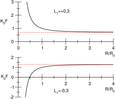
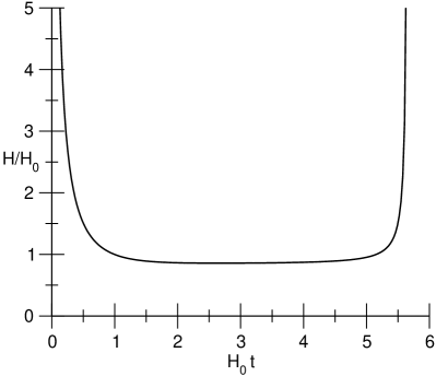
Figure 4: Corresponding to Sec. 5.5 we plot (a) the function $K_{0}F=L_{0}-+L\frac{R_{0}^{2}}{R^{2}}$ for $L_{1}=\pm 0,3$ and (b) the Hubble scale $H(t)$ for $L_{1}=+0,1$; $R_{0}=1,1$; $\Omega_{\Lambda 0}=0,73$ and $Q=\frac{1}{2}$ (dust), where a Big Rip singularity occurs.

5.6 $\boldsymbol{\Lambda G=\Lambda_{0}G_{0}\frac{\mu^{2}}{\mu_{0}^{2}}}$, $\boldsymbol{\mu=R^{-1}}$

Here, one cannot find a prediction for $R_{\text{e}}$ in the de Sitter limit ($\dot{H}=0$, $R\rightarrow R_{\text{e}}=H_{\text{e}}^{-1}$) since Eq. (10) only leads to the constraint $R_{0}^{2}=1/(H_{0}^{2}\Omega_{\Lambda 0})$. To find solutions corresponding to other values of $R_{0}$ we impose the ansatz $a(t)=a_{0}(t-t_{1})^{n}$ with $a_{0},n,t_{1}=\text{const}$. The Hubble scale is given by $H=n(t-t_{1})^{-1}$ which implies due to $H_{0}>0$ that $t_{1}<t$ for $n>0$ and $t_{1}>t$ for $n<0$, respectively. For $0<n<1$ the event horizon does not exist, in the other cases $R$ can be calculated exactly via Eq. (6):

$$R(t)=a(t)\int_{t}^{t_{\text{E}}}\frac{\text{d}t^{\prime}}{a(t^{\prime})}=(t-t_{1})^{n}\cdot\frac{(t_{\text{E}}-t_{1})^{(1-n)}-(t-t_{1})^{(1-n)}}{1-n}.$$

Note that for negative $n$ there is a Big Rip singularity at $t\rightarrow t_{1}$, where $a(t)$ diverges and the universe ends: $t_{\text{E}}=t_{1}$. For $n>1$ the scale factor $a(t)$ describes power-law acceleration and there is no future singularity which means $t_{\text{E}}\rightarrow\infty$. As a result, both cases yield

$$R(t)=\frac{(t-t_{1})}{n-1}.$$

Thus Eq. (10) can be solved exactly, which determines the constant $n$, see Fig. 5:

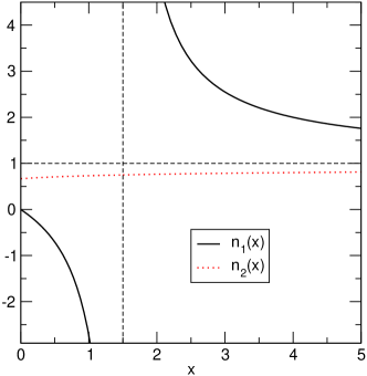
Figure 5: The exponents $n_{1,2}(x)$ from Eq. (15), which occur in the power-law expansion scale factor $a(t)=a_{0}(t-t_{1})^{n}$, are shown. In Sec. 5.6 we find $n=n_{1}(R_{0}^{2}/K_{0})$, whereas $n=n_{2}(T_{0}^{2}/K_{0})$ in Sec. 5.9.

$$n_{1,2}(x) = \frac{(x-\frac{1}{2})\pm\sqrt{(x-\frac{1}{2})^{2}-x(x-(Q+1))}}{x-(Q+1)}$$ (15)

$$\text{with}\,\,x := \frac{R_{0}^{2}}{K_{0}}=R_{0}^{2}H_{0}^{2}\Omega_{\Lambda 0}(Q+1).$$ (16)

For $Q>0$ we find $(Q+1)^{-1}<n_{2}<1$ for all positive values of $x$, therefore $n_{2}$ can be dropped as the event horizon does not exist. In the case $R_{0}^{2}<1/(H_{0}^{2}\Omega_{\Lambda 0})$ the constant $n=n_{1}$ is negative leading to a Big Rip singularity at the time $t=t_{1}$, and $R_{0}^{2}>1/(H_{0}^{2}\Omega_{\Lambda 0})$ implies a positive $n$ corresponding to power-law acceleration.

5.7 $\boldsymbol{\Lambda=\Lambda_{0}(1-q_{1}\ln\frac{\mu}{\mu_{0}})}$, $\boldsymbol{\mu=T^{-1}}$

Solving Eq. (10) for this choice of $\Lambda$ and $\mu$ can be done approximately. First we propose the ansatz $a(t)=a_{0}\exp(u^{2}(t-t_{1})^{2})$ for the scale factor with the constants $a_{0}$, $u$ and $t_{1}$. Therefore

$$H=2u^{2}(t-t_{1}),\,\,\,\,\frac{\ddot{a}}{a}=4u^{4}(t-t_{1})^{2}+2u^{2},\,\,\,\,F=2u^{2}+4u^{4}(Q+1)(t-t_{1})^{2},$$

and the particle horizon radius at late times reads

$$T = \exp(u^{2}(t-t_{1})^{2})\int_{t_{x}}^{t}\exp(-u^{2}(t^{\prime}-t_{1})^{2})\text{d}t^{\prime},\,\,\,\,t>t_{x}=\text{const.}$$

$$= \exp(u^{2}(t-t_{1})^{2})\cdot\left[\frac{\sqrt{\pi}}{2u}\text{erf}(u(t-t_{1}))\right]_{t_{x}}^{t}.$$

For $t\rightarrow\infty$ the series expansion of the square brackets reads $C+\mathcal{O}(t^{-1})$ with $C>0$ and thus $T\approx C\exp(u^{2}(t-t_{1})^{2})$. In this limit the given ansatz for $a(t)$ solves $K_{0}F=1-q_{1}\ln\frac{T_{0}}{T}$ exactly and determines the constant $u^{2}=\frac{1}{4}q_{1}H_{0}^{2}\Omega_{\Lambda 0}$. Therefore we have found an approximate late-time solution in the case $q_{1}>0$.

The numerical solutions in the case $q_{1}<0$ exhibits a future Big Crunch singularity. At times sufficiently before this event the scale factor can be well approximated by the ansatz $a(t)=a_{0}\exp(-u^{2}(t-t_{1})^{2})$, which implies $F=-2u^{2}+4u^{4}(Q+1)(t-t_{1})^{2}$ and

$$T=\exp(-u^{2}(t-t_{1})^{2})\cdot\left[\frac{\sqrt{\pi}}{2iu}\text{erf}(iu(t-t_{1}))\right]_{t_{x}}^{t},\,\,\,\,t>t_{x}=\text{const}.$$

We expand the square bracket term around $t\rightarrow t_{1}$, where the scale factor is maximal, and find $T\approx C\exp(-u^{2}(t-t_{1})^{2})$ with $C>0$. Solving $K_{0}F=1-q_{1}\ln\frac{T_{0}}{T}$ leads to $u^{2}=-\frac{1}{4}q_{1}H_{0}^{2}\Omega_{\Lambda 0}$ in accordance with $q_{1}<0$. The numerical and approximate solutions are shown in Fig. 6.

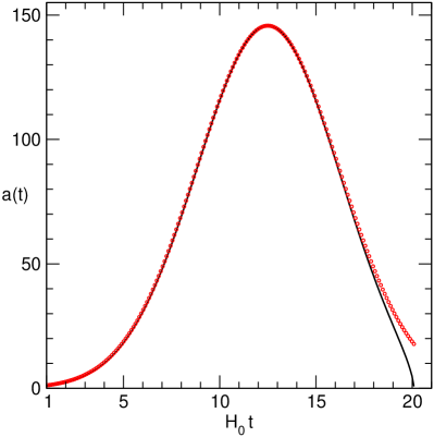
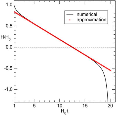
Figure 6: Here, the numerical and the approximate solutions for the scale factor $a(t)$ and the Hubble scale $H(t)$ from Sec. 5.7 are shown for negative $q_{1}=-0,2$. Furthermore, we used $\Omega_{\Lambda 0}=0,73$; $T_{0}H_{0}=3$ and $Q=\frac{1}{2}$ (dust). In this case a Big Crunch singularity will occur in the future. Note that the analytical approximation works very well except near the future singularity.

5.8 $\boldsymbol{\Lambda=\Lambda_{0}(L_{0}+L_{1}\frac{\mu^{2}}{\mu_{0}^{2}})}$, $\boldsymbol{\mu=T^{-1}}$

In the late-time de Sitter limit, $a(t)\propto\exp(H_{\text{e}}t)$, the particle horizon radius has the asymptotic form

$$T\propto\exp(H_{\text{e}}t)\rightarrow\infty\,\,\,\,\text{for}\,\,\,\,t\rightarrow\infty,$$

which follows from Eq. (8). This means that $K_{0}F\rightarrow L_{0}$ and thus determines $H_{\text{e}}^{2}=H_{0}^{2}\Omega_{\Lambda 0}L_{0}$. To verify the stability of this solution we calculate

$$K_{0}\dot{F}=-2L_{1}\frac{\dot{T}}{T}\cdot\frac{T_{0}^{2}}{T^{2}}=-2L_{1}\frac{T_{0}^{2}}{T^{2}}\left(H+\frac{1}{T}\right)\!\!.$$

At the initial time (today) $K_{0}\dot{F}$ is negative for $L_{1}>0$ and $K_{0}F$ keeps on approaching the de Sitter limit unless a sign change in $K_{0}\dot{F}$ would occur. But this requires a negative $H$, which is only possible if $K_{0}F=\dot{H}+(Q+1)H^{2}<0$ at some time. Since $K_{0}F\geq L_{0}>0$ we conclude that the de Sitter limit will be reached always. For $L_{1}<0$ the initial values of $K_{0}F$ and $K_{0}\dot{F}$ are positive and $K_{0}F$ approaches the de Sitter limit. Again, a sign change in $K_{0}\dot{F}$ is only possible for $H<0$, which requires $K_{0}F<0$ at some time. These conditions cannot be realised because $K_{0}F>0$ as long as $K_{0}\dot{F}>0$. In summary all reasonable values of $L_{1}$ lead to a stable de Sitter final state.

5.9 $\boldsymbol{\Lambda G=\Lambda_{0}G_{0}\frac{\mu^{2}}{\mu_{0}^{2}}}$, $\boldsymbol{\mu=T^{-1}}$

By using at late times the ansatz $a(t)=a_{0}(t-t_{1})^{n}$ with $a_{0},t,n=\text{const.}$, we find

$$F=(n^{2}(Q+1)-n)(t-t_{1})^{-2},$$

and the particle horizon radius is given by

$$T=a_{0}(t-t_{1})^{n}\left[\int_{0}^{t_{0}}\frac{\text{d}t^{\prime}}{a(t^{\prime})}+\int_{t_{0}}^{t}\frac{\text{d}t^{\prime}}{a(t^{\prime})}\right]=\frac{t-t_{1}}{1-n}+(t-t_{1})^{n}\left[T_{0}-\frac{(t_{0}-t_{1})^{1-n}}{1-n}\right]\!\!,$$ (17)

where $T_{0}=T(t_{0})>0$ depends on the past evolution of the scale factor. In the case $n<0$ a positive Hubble scale $H=n(t-t_{1})^{-1}$ requires $t,t_{0}<t_{1}$, which implies $T<0$ and thus the non-existence of the particle horizon. For $0<n<1$ the second term in Eq. (17) can be neglected at late times, and Eq. (10) can be solved exactly, leading to

$$n_{1,2}(x) = \frac{(x-\frac{1}{2})\pm\sqrt{(x-\frac{1}{2})^{2}-x(x-(Q+1))}}{x-(Q+1)}$$

$$\text{with}\,\,x := \frac{T_{0}^{2}}{K_{0}}=T_{0}^{2}H_{0}^{2}\Omega_{\Lambda 0}(Q+1).$$

This is the same equation as in Sec. 5.6 with $R_{0}$ replaced by $T_{0}$, see also Fig. 5. Here, solution $n_{2}$ is the physical one because of $(Q+1)^{-1}<n_{2}<1$, that corresponds to a decelerating universe for $t\rightarrow\infty$. In comparison with Sec. 5.6 the identification of the particle horizon radius as renormalisation scale yields a complementary cosmological behaviour.

6 Conclusions

In this work we have studied the effect of a variable CC on the late-time evolution of the universe. Thereby the variability of the CC originates from RGEs that are provided by certain quantum theories, leading to a scale-dependence of the CC. By identifying the renormalisation scale with cosmologically relevant scales, the CC becomes effectively time-dependent. In contrast to many other models of DE, here, the EOS is still that of a classical CC, which implies a non-trivial scaling behaviour of the cosmological matter content. Concretely, we have investigated three RGEs for the CC and three choices for the renormalisation scale: the Hubble scale and the inverse radii of the cosmological event horizon and particle horizon. For one RGE we have also included the renormalisation group running of Newton’s constant. In all cases we have determined the possible final states of the universe and discussed their properties. Depending on the choice of the initial conditions and parameters, we have found at late times asymptotic de Sitter solutions, accelerating and decelerating power-law solutions and super-exponential expansion laws of the type $a(t)\sim\exp(ct^{2})$. Additionally, we have encountered future singularities of the Big Rip and Big Crunch type. However, some solutions should be treated with caution, since they imply physically questionable results like negative energy densities. Also, the cosmological behaviour near future singularities might get altered by additional effects, that have not been taken into account in this work. It was shown, for instance, in Refs. [30] that quantum effects are able to prevent or weaken future singularities. Moreover, higher-derivative terms in the gravitational action and a time-dependent Newton’s constant could potentially change the solutions.

Nevertheless, we stay in this analysis on the basic level and use the results we found as an indicator for the (in)stability of the cosmological fate. Indeed, we have found regular solutions in many cases, which can be considered as realisable in nature. In this sense, we have found de Sitter solutions in Secs. 5.1, 5.2, 5.4 and 5.8. Also the power-law solutions can be called regular, they appear for all cases with the scaling law (3) in Secs. 5.3, 5.3 and 5.9. Moreover, we have found super-exponential expansion laws in Sec. 5.7. Big Rip type future singularities exist for all cases with the event horizon as renormalisation scale, see Secs. 5.4, 5.5 and 5.6. Big Crunch solutions, on the other hand, occur only for the scaling law (1) as described in Secs. 5.1, 5.4 and 5.7. Finally, a comprehensive overview of our results is given in Tab. 1. Since some solution types occur only for certain combinations of scaling laws and scales, our analysis helps to discriminate between the different cases and discover the nature of DE.

	$\Lambda=\Lambda_{0}(1-q_{1}\ln\frac{\mu}{\mu_{0}})$	$\Lambda=\Lambda_{0}(L_{0}+L_{1}\frac{\mu^{2}}{\mu_{0}^{2}})$	$\Lambda G=\Lambda_{0}G_{0}\frac{\mu^{2}}{\mu_{0}^{2}}$
$\mu=H$	dS, BC	dS	P
$\mu=R^{-1}$	dS, BR, BC	BR	P, BR
$\mu=T^{-1}$	$\exp(\pm t^{2})$, BC	dS	P

Table 1: This table shows all types of cosmological final states that we have found in Sec. 5 for the all combinations of scaling laws for the CC $\Lambda$ (and $G$ for the third law) from Sec. 2 and the choices for the renormalisation scale $\mu$ of Sec. 3. Here, dS denotes de Sitter solutions, P power-law solutions, BR Big Rip and BC Big Crunch future singularities, respectively. With $\exp(\pm t^{2})$ we mean the late-time behaviour of the scale factor, where $a\propto\exp(-t^{2})$ finally leads to a Big Crunch.

In a future work, we would like to discuss the consequences of a running CC for the early universe, too.

References

- [1] Supernova Search Team Collaboration, A. G. Riess et al., Astron. J. 116, 1009 (1998), astro-ph/9805201; J. L. Tonry et al., Astrophys. J. 594, 1 (2003), astro-ph/0305008.
- [2] Supernova Cosmology Project Collaboration, S. Perlmutter et al., Astrophys. J. 517, 565 (1999), astro-ph/9812133; R. A. Knop et al., Astrophys. J. 598, 102 (2003), astro-ph/0309368.
- [3] WMAP Collaboration, D. N. Spergel et al., Astrophys. J. Suppl. 148, 175 (2003), astro-ph/0302209.
- [4] SDSS Collaboration, M. Tegmark et al., Phys. Rev. D 69, 103501 (2004), astro-ph/0310723.
- [5] S. P. Boughn and R. G. Crittenden, Nature 427, 45 (2004), astro-ph/0404470.
- [6] S. Hannestad, astro-ph/0509320.
- [7] P. J. E. Peebles and B. Ratra, Rev. Mod. Phys. 75 (2003) 559, astro-ph/0207347.
- [8] V. Sahni, Lect. Notes Phys. 653 (2004) 141, astro-ph/0403324.
- [9] T. Padmanabhan, Phys. Rept. 380 (2003) 235, hep-th/0212290; T. Padmanabhan, gr-qc/0503107; T. Padmanabhan, astro-ph/0510492.
- [10] S. Weinberg, Rev. Mod. Phys. 61, 1 (1989).
- [11] N. D. Birrell and P. C. W. Davies, “Quantum Fields In Curved Space,” Cambridge, UK: Univ. Pr. (1982) 340p.; I. L. Buchbinder, S. D. Odintsov and I. L. Shapiro, “Effective action in quantum gravity,” Bristol, UK: IOP (1992) 413 p.
- [12] I. L. Shapiro, J. Sola, Phys. Lett. B 475 (2000) 236, hep-ph/9910462; I. L. Shapiro, J. Sola, JHEP 0202 (2002) 006, hep-th/0012227; A. Babic, B. Guberina, R. Horvat, H. Stefancic, Phys. Rev. D 65 (2002) 085002, hep-ph/0111207; B. Guberina, R. Horvat, H. Stefancic, Phys. Rev. D 67 (2003) 083001, hep-ph/0211184; I. L. Shapiro, J. Sola, C. Espana-Bonet, P. Ruiz-Lapuente, Phys. Lett. B 574 (2003) 149, astro-ph/0303306; I. L. Shapiro, J. Sola, Nucl. Phys. Proc. Suppl. 127 (2004) 71, hep-ph/0305279; C. Espana-Bonet, P. Ruiz-Lapuente, I. L. Shapiro, J. Sola, JCAP 0402 (2004) 006, hep-ph/0311171; A. Babic, B. Guberina, R. Horvat, H. Stefancic, Phys. Rev. D 71 (2005) 124041, astro-ph/0407572; I. L. Shapiro, J. Sola, astro-ph/0401015; I. L. Shapiro, J. Sola, H. Stefancic, JCAP 0501 (2005) 012, hep-ph/0410095; B. Guberina, R. Horvat, H. Stefancic, JCAP 0505 (2005) 001, astro-ph/0503495.
- [13] M. Reuter, Phys. Rev. D 57 (1998) 971, hep-th/9605030; A. Bonanno and M. Reuter, Phys. Rev. D 65 (2002) 043508, hep-th/0106133.
- [14] M. Reuter, C. Wetterich, Phys. Lett. B 188 (1987) 38; M. Reuter, hep-th/0012069; D. F. Litim, Phys. Rev. D 64 (2001) 105007 hep-th/0103195; A. Bonanno, M. Reuter, Int. J. Mod. Phys. D 13 (2004) 107, astro-ph/0210472; A. Bonanno, G. Esposito, C. Ruban, Gen. Rel. Grav. 35 (2003) 1899, hep-th/0303154; M. Reuter, H. Weyer, hep-th/0311196; A. Bonanno, G. Esposito, C. Rubano, gr-qc/0403115; M. Reuter, H. Weyer, JCAP 0412 (2004) 001, hep-th/0410119; M. Reuter, H. Weyer, Phys. Rev. D 70 (2004) 124028, hep-th/0410117; J. W. Moffat, astro-ph/0412195.
- [15] O. Bertolami, J. M. Mourao, J. Perez-Mercader, Phys. Lett. B 311 (1993) 27; E. Elizalde, S. D. Odintsov, I. L. Shapiro, Class. Quant. Grav. 11 (1994) 1607, hep-th/9404064; O. Bertolami, J. Garcia-Bellido, Int. J. Mod. Phys. D 5 (1996) 363, astro-ph/9502010; E. Elizalde, C. O. Lousto, S. D. Odintsov, A. Romeo, Phys. Rev. D 52 (1995) 2202, hep-th/9504014; S. Falkenberg, S. D. Odintsov, Int. J. Mod. Phys. A 13 (1998) 607, hep-th/9612019; A. A. Bytsenko, L. N. Granda, S. D. Odintsov, JETP Lett. 65 (1997) 600, hep-th/9705008; L. N. Granda, S. D. Odintsov, Grav. Cosmol. 4 (1998) 85, gr-qc/9801026; E. Verlinde, H. Verlinde, JHEP 0005 (2000) 034, hep-th/9912018; C. Rubano, P. Scudellaro, Gen. Rel. Grav. 37 (2005) 521, astro-ph/0410260; H. W. Hamber, R. M. Williams, Phys. Rev. D 72 (2005) 044026, hep-th/0507017; G. V. Vereshchagin, astro-ph/0511131.
- [16] C. Wetterich, Nucl. Phys. B 302, 668 (1988); B. Ratra and P. J. E. Peebles, Phys. Rev. D 37, 3406 (1988).
- [17] C. Espana-Bonet, P. Ruiz-Lapuente, hep-ph/0503210; R. Lazkoz, S. Nesseris, L. Perivolaropoulos, astro-ph/0503230; H. Stefancic, Phys. Rev. D 71 (2005) 124036, astro-ph/0504518; H. K. Jassal, J. S. Bagla, T. Padmanabhan, Phys. Rev. D 72 (2005) 103503, astro-ph/0506748; D. Polarski, A.Ranquet, Phys. Lett. B 627 (2005) 1, astro-ph/0507290; S. Capozziello, V. F. Cardone, E. Elizalde, S. Nojiri, S. D. Odintsov, astro-ph/0508350; V. B. Johri, P. K. Rath, astro-ph/0510017; B. M. N. Carter, I. P. Neupane, hep-th/0510109; S. Nojiri, S. D. Odintsov, O. G. Gorbunova, hep-th/0510183; S. Nesseris, L. Perivolaropoulos, astro-ph/0511040; J. Ren, X. H. Meng, astro-ph/0511163; H. Stefancic, astro-ph/0511316.
- [18] J. Sola, H. Stefancic, Phys. Lett. B 624 (2005) 147, astro-ph/0505133; J. Sola, H. Stefancic, astro-ph/0507110.
- [19] F. Bauer, Class. Quant. Grav. 22 (2005) 3533, gr-qc/0501078.
- [20] E. V. Gorbar, I. L. Shapiro, JHEP 0302 (2003) 021, hep-ph/0210388. I. L. Shapiro, hep-th/0412115.
- [21] O. Lauscher, M. Reuter, Phys. Rev. D 65 (2002) 025013, hep-th/0108040; O. Lauscher, M. Reuter, Class. Quant. Grav. 19 (2002) 483, hep-th/0110021; D. F. Litim, Phys. Rev. Lett. 92 (2004) 201301, hep-th/0312114; J. A. Belinchon, T. Harko, M. K. Mak, Class. Quant. Grav. 19 (2002) 3003, gr-qc/0108074.; A. Bonanno, M. Reuter, hep-th/0410191; A. Bonanno, G. Esposito, G. Rubano, P. Scudellaro, astro-ph/0507670; A. Bonanno, G. Esposito, C. Rubano, Int. J. Mod. Phys. A 20 (2005) 2358, hep-th/0511188.
- [22] A. Bonanno, M. Reuter, Phys. Lett. B 527 (2002) 9, astro-ph/0106468; E. Bentivegna, A. Bonanno, M. Reuter, JCAP 0401 (2004) 001, astro-ph/0303150.
- [23] M. Reuter, F. Saueressig, JCAP 0509 (2005) 012, hep-th/0507167.
- [24] H. W. Hamber, R. M. Williams, Nucl. Phys. B 435, 361 (1995), hep-th/9406163; H. W. Hamber, R. M. Williams, Phys. Rev. D 59, 064014 (1999), hep-th/9708019; H. W. Hamber, Phys. Rev. D 61, 124008 (2000), hep-th/9912246.
- [25] G. W. Gibbons, S. W. Hawking, Phys. Rev. D 15 (1977) 2738; T. Padmanabhan, Phys. Rept. 406 (2005) 49, gr-qc/0311036.
- [26] T. M. Davis, C. H. Lineweaver, astro-ph/0310808.
- [27] S. D. H. Hsu, Phys. Lett. B 594 (2004) 13, hep-th/0403052; M. Li, Phys. Lett. B 603 (2004) 1, hep-th/0403127; R. Horvat, Phys. Rev. D 70 (2004) 087301, astro-ph/0404204; Q. G. Huang, M. Li, JCAP 0408 (2004) 013, astro-ph/0404229; S. Carneiro, J. A. S. Lima, Int. J. Mod. Phys. A 20 (2005) 2465, gr-qc/0405141; E. Elizalde, S. Nojiri, S. D. Odintsov, P. Wang, Phys. Rev. D 71 (2005) 103504, hep-th/0502082; Y. S. Myung, Phys. Lett. B 626 (2005) 1, hep-th/0502128; Y. g. Gong, Y. Z. Zhang, Class. Quant. Grav. 22 (2005) 4895, hep-th/0505175; G. Izquierdo, D. Pavon, astro-ph/0505601; B. Wang, Y. g. Gong, E. Abdalla, Phys. Lett. B 624 (2005) 141, hep-th/0506069; S. Nojiri, S. D. Odintsov, hep-th/0506212; B. Guberina, R. Horvat, H. Nikolic, astro-ph/0507666; P. F. Gonzalez-Diaz, astro-ph/0507714; H. Kim, H. W. Lee, Y. S. Myung, gr-qc/0509040; D. Pavon, W. Zimdahl, hep-th/0511053; B. Wang, Y. Gong, E. Abdalla, gr-qc/0511051.
- [28] L. Parker, Phys. Rev. Lett. 21 (1968) 562.
- [29] J. D. Barrow, Class. Quant. Grav. 21 (2004) L79, gr-qc/0403084; H. Stefancic, Phys. Rev. D 71 (2005) 084024, astro-ph/0411630; S. Nojiri, S. D. Odintsov, S. Tsujikawa, Phys. Rev. D 71 (2005) 063004, hep-th/0501025; M. Sami, A. Toporensky, P. V. Tretjakov, S. Tsujikawa, Phys. Lett. B 619 (2005) 193, hep-th/0504154; P. Tretyakov, A. Toporensky, C. Cattoen, M. Visser, gr-qc/0508045; Y. Shtanov, V. Sahni, gr-qc/0510104.
- [30] S. Nojiri, S. D. Odintsov, Phys. Lett. B 595 (2004) 1, hep-th/0405078; S. Nojiri, S. D. Odintsov, Phys. Rev. D 70 (2004) 103522, hep-th/0408170; E. Elizalde, S. Nojiri, S. D. Odintsov, Phys. Rev. D 70 (2004) 043539, hep-th/0405034.