Explicit solutions for relativistic acceleration and rotation

Abstract

The Lorentz transformations are represented by Einstein velocity addition on the ball of relativistically admissible velocities. This representation is by projective maps. The Lie algebra of this representation defines the relativistic dynamic equation. If we introduce a new dynamic variable, called symmetric velocity, the above representation becomes a representation by conformal, instead of projective maps. In this variable, the relativistic dynamic equation for systems with an invariant plane, becomes a non-linear analytic equation in one complex variable. We obtain explicit solutions for the motion of a charge in uniform, mutually perpendicular electric and magnetic fields. By assuming the Clock Hypothesis and using these solutions, we are able to describe the space-time transformations between two uniformly accelerated and rotating systems.

PACS: 04.90.+e; 03.30.+p.

Keywords: Relativistic accelerated systems; Explicit space-time transformation between accelerated systems.

1 Representation of the Lorentz transformations on the ball of relativistically admissible velocities

The usual Lorentz space-time transformations between two inertial systems $K$ and $K^{\prime}$, moving with relative velocity (boost) $\mathbf{b}$. The space axes are chosen to be parallel. The Lorentz transformation $L$ transforms the space-time coordinates $(t,\mathbf{r})$ in $K$ of an event to the space-time coordinates $(t^{\prime},\mathbf{r}^{\prime})$ in $K^{\prime}$ of the same event. If we assume that the interval $ds^{2}=(cdt)^{2}-d\mathbf{r}^{2}$ is conserved, the resulting space-time transformation between systems is called the Lorentz transformation. In the case $\mathbf{b}=(b,0,0)$ the Lorentz transformation $L_{v}$ from system $K^{\prime}$ to system $K$ is

$$\begin{array}[]{cl}t&=\gamma(t^{\prime}+\frac{bx^{\prime}}{c^{2}})\\ x&=\gamma(bt^{\prime}+x^{\prime})\\ y&=y^{\prime}\\ z&=z^{\prime},\end{array}$$ (1)

with $\gamma=\frac{1}{\sqrt{1-b^{2}/c^{2}}}.$

This Lorentz transformation for arbitrary relative velocity $\mathbf{b}$ can be rewritten in the vector and block-matrix notation as:

$$\left(\begin{array}[]{c}t\\ \mathbf{r}\end{array}\right)=L_{\mathbf{b}}\left(\begin{array}[]{c}t^{\prime}\\ \mathbf{r}^{\prime}\end{array}\right)=\left(\begin{array}[]{cc}\gamma&\gamma c^{-2}\mathbf{b}^{T}\\ \gamma\mathbf{b}&\gamma P_{\mathbf{b}}+(I-P_{\mathbf{b}})\end{array}\right)\left(\begin{array}[]{c}t^{\prime}\\ \mathbf{r}^{\prime}\end{array}\right)$$ (2)

or

$$L_{\mathbf{b}}\left(\begin{array}[]{c}t^{\prime}\\ \mathbf{r}^{\prime}\end{array}\right)=\gamma\left(\begin{array}[]{cc}1&c^{-2}\mathbf{b}^{T}\\ \mathbf{b}&P_{\mathbf{b}}+\alpha(I-P_{\mathbf{b}})\end{array}\right)\left(\begin{array}[]{c}t^{\prime}\\ \mathbf{r}^{\prime}\end{array}\right),$$ (3)

where

$$\alpha=\gamma^{-1}=\sqrt{1-|\mathbf{b}|^{2}/c^{2}}$$ (4)

and $P_{\mathbf{b}}$ is the orthogonal projection on the direction of $\mathbf{b}$ defined by $P_{\mathbf{b}}\mathbf{r}=\frac{\langle\mathbf{b}|\mathbf{r}\rangle}{|\mathbf{b}|^{2}}\mathbf{b}$.

From this formula one derives the velocity addition as follows. Consider motion with uniform velocity $\mathbf{u}$ in system $K^{\prime}$. The world line of this motion is $\left(\begin{array}[]{c}t^{\prime}\\ \mathbf{u}t^{\prime}\end{array}\right).$ By use of (3) this world line in system $K$ is

$$\gamma\left(\begin{array}[]{c}t^{\prime}+\frac{\mathbf{b}^{T}\mathbf{u}t^{\prime}}{c^{2}}\\ \mathbf{b}t^{\prime}+t^{\prime}P_{\mathbf{b}}\mathbf{u}+\alpha t^{\prime}(I-P_{\mathbf{b}})\mathbf{u}\end{array}\right)$$ (5)

or

$$\gamma t^{\prime}\left(\begin{array}[]{c}1+\frac{\langle\mathbf{b}|\mathbf{u}\rangle}{c^{2}}\\ \mathbf{b}+\mathbf{u}_{\|}+\alpha\mathbf{u}_{\bot}\end{array}\right),$$ (6)

where $\mathbf{u}_{\|}=P_{\mathbf{b}}\mathbf{u}$ denote the component of $\mathbf{u}$ parallel to $\mathbf{b}$ and $\mathbf{u}_{\bot}=(I-P_{\mathbf{b}})\mathbf{u}$ denote the component of $\mathbf{u}$ perpendicular to $\mathbf{b}.$ This define a uniform motion in system $K$ with velocity, called the relativistic velocity sum $\mathbf{b}\oplus\mathbf{u}.$ Thus, we get

$$\mathbf{b}\oplus\mathbf{u}=\frac{\mathbf{b}+\mathbf{u}_{\|}+\alpha\mathbf{u}_{\bot}}{1+\frac{\langle\mathbf{b}|\mathbf{u}\rangle}{c^{2}}},$$ (7)

which is the well-known Einstein velocity addition formula.

In case $\mathbf{b}$ and $\mathbf{u}$ are parallel, this formula become:

$$\mathbf{b}\oplus\mathbf{u}=\frac{\mathbf{b}+\mathbf{u}}{1+\frac{{b}{u}}{c^{2}}},$$ (8)

and in case $\mathbf{u}$ is perpendicular to $\mathbf{b}$ the formula become:

$$\mathbf{b}\oplus\mathbf{u}=\mathbf{b}+\alpha(\mathbf{b})\mathbf{u}.$$ (9)

Note that the velocity addition is commutative only for parallel velocities.

We denote by $D_{v}$ the set of all relativistically admissible velocities in an inertial frame $K$. This set is defined by

$$D_{v}=\{\mathbf{v}:\;\mathbf{b}\in R^{3},\;|\mathbf{b}|<c\}.$$ (10)

The Lorentz transformation (3) acts on the velocity ball $D_{v}$ as

$$\varphi_{\mathbf{b}}(\mathbf{v})=\mathbf{b}\oplus\mathbf{v}=\frac{\mathbf{b}+\mathbf{u}_{\|}+\alpha\mathbf{u}_{\bot}}{1+\frac{\langle\mathbf{b}|\mathbf{v}\rangle}{c^{2}}},$$ (11)

with $\alpha$ defined by (4). It can be shown [4] that the map $\varphi_{\mathbf{b}}$ is a projective (preserving line segments) map of $D_{v}$.

We denote by $Aut_{p}(D_{v})$ the group of all projective automorphisms of the domain $D_{v}$. The map $\varphi_{\mathbf{b}}$ belongs to $Aut_{p}(D_{v})$ and transforms any relativistically admissible velocity $\mathbf{v}\in D_{v}$ of the system $K^{\prime}$, which is moving parallel to $K$ with relative velocity $\mathbf{b}$, to a corresponding unique velocity $\varphi_{\mathbf{b}}(\mathbf{v})\in D_{v}$ in $K$. Let $\psi$ be any projective automorphism of $D_{v}$. Set $\mathbf{b}=\psi(0)$ and $U=\varphi_{\mathbf{b}}^{-1}\psi$. Then $U$ is an isometry and represented by an orthogonal matrix. Thus, the group $Aut_{p}(D_{v})$ of all projective automorphisms is

$$Aut_{p}(D_{v})=\{\varphi_{\mathbf{b},U}=\varphi_{\mathbf{b}}U:\mathbf{b}\in D_{v},\;U\in O(3)\}.$$ (12)

This group represent the velocity transformation between arbitrary two inertial systems and provide a representation of the Lorentz group.

Note that the Lorentz group representation defined by space-time transformations (3) between two inertial systems is valid only if at time $t=0$ the origins of the two systems coincide, while the velocity transformation (12) between two inertial systems holds for arbitrary systems without any limitation.

2 Relativistic dynamics

It is well known that a force generates a velocity change, or acceleration. There are two types of forces. The first type generates changes in the magnitude of the velocity and can be considered a velocity boost. An example is the force of an electric field on a charged particle. The second type of force generates a change in the direction of the velocity - a rotation or, equivalently, acceleration in a direction perpendicular to the velocity of the object. An example is a magnetic field acting on a moving charge. Thus a force can be considered as a generator of velocity change. During the time evolution, the velocity of an object cannot leave the velocity ball $D_{v}$. Therefore, it is natural to assume that the generator of a relativistic evolution is an element of the Lie algebra $aut_{p}(D_{v})$, which consists of the generators of the group $Aut_{p}(D_{v})$ generated by velocity addition. We will call a relativistic motion generated by a constant uniform force motion with uniform acceleration.

To define the elements of $aut_{p}(D_{v})$, consider differentiable curves $g(s)$ from a neighborhood $I_{0}$ of $0$ into $Aut_{p}(D_{v})$, with $g(0)=\varphi_{0,I}$, the identity of $Aut_{p}(D_{v})$. Any such $g(s)$ has the form

$$g(s)=\varphi_{\mathbf{b}(s),U(s)},$$ (13)

where $\mathbf{b}:I_{0}\rightarrow D_{v}$ is a differentiable function satisfying $\mathbf{b}(0)=\mathbf{0}$ and $U(s):I_{0}\rightarrow O(3)$ is differentiable and satisfies $U(0)=I$. We denote by $\delta$ the element of $aut_{p}(D_{v})$ generated by $g(s)$. By direct calculation (see [4]) we get

$$\delta(\mathbf{v})=\frac{d}{ds}g(s)(\mathbf{v})\Bigr{|}_{s=0}=\mathbf{E}+A\mathbf{v}-c^{-2}\langle\mathbf{v}|\mathbf{E}\rangle\mathbf{v},$$ (14)

where $\mathbf{E}=\mathbf{b}^{\prime}(0)\in R^{3}$ and $A=U^{\prime}(0)$ is $3\times 3$ skew-symmetric matrix. Defining $\mathbf{B}=\left(\begin{array}[]{c}a_{23}\\ -a_{13}\\ a_{12}\end{array}\right)$, we have

$$A\mathbf{v}=\mathbf{v}\times\mathbf{B},$$ (15)

where $\times$ denotes the vector product in $R^{3}$. Thus, the Lie algebra

$$aut_{p}(D_{v})=\{\delta_{\mathbf{E},\mathbf{B}}:\mathbf{E},\mathbf{B}\in R^{3}\},$$ (16)

where $\delta_{\mathbf{E},\mathbf{B}}:D_{v}\rightarrow R^{3}$ is the vector field defined by

$$\delta_{\mathbf{E},\mathbf{B}}(\mathbf{v})=\mathbf{E}+\mathbf{v}\times\mathbf{B}-c^{-2}\langle\mathbf{v}\,|\mathbf{E}\rangle\mathbf{v}.$$ (17)

Note that any $\delta(\mathbf{v})$ is a polynomial in $\mathbf{v}$ of degree less than or equal to 2. The elements of $aut_{p}(D_{v})$ transform between two inertial systems in the same way as the electromagnetic field strength.

Evolution described by a relativistic dynamic equation must preserve the ball $D_{v}$ of all relativistically admissible velocities. If we consider the force as an element of $aut_{p}(D_{v})$, the equation of evolution of a charged particle with charge $q$ and rest-mass $m_{0}$ using the generator $\delta_{\mathbf{E},\mathbf{B}}\in aut_{p}(D_{v})$ is defined by

$$\frac{d\mathbf{v}(\tau)}{d\tau}=\frac{q}{m_{0}}\delta_{\mathbf{E},\mathbf{B}}(\mathbf{v}(\tau)),$$ (18)

or

$$\frac{d\mathbf{v}(\tau)}{d\tau}=\frac{q}{m_{0}}(\mathbf{E}+\mathbf{v}(\tau)\times\mathbf{B}-c^{-2}\langle\mathbf{v}(\tau)|\mathbf{E}\rangle\mathbf{v}(\tau)),$$ (19)

where $\tau$ is the proper time of the particle. It can be shown that this formula coincides with the well-known formula

$$\frac{d(m\mathbf{v})}{dt}=q(\mathbf{E}+\mathbf{v}\times\mathbf{B}).$$

Thus, the flow generated by an electromagnetic field is defined by elements of the Lie algebra $aut_{p}(D_{v})$, which are, in turn, vector field polynomials in $\mathbf{v}$ of degree 2. The linear term of this field comes from the magnetic force, while the constant and the quadratic terms come from the electric field. If the electromagnetic field $\mathbf{E},\mathbf{B}$ is constant, for any given $\tau$ the solution of (19) is an element $\varphi_{\mathbf{b}(\tau),U(\tau)}\in Aut_{p}(D_{v})$ and the set of such elements form a one-parameter subgroup of $Aut_{p}(D_{v})$. This subgroup is a geodesic under the invariant metric on the group. It can be shown by same argument (if we set $\mathbf{B}=0$) that the dynamic equation of evolution in relativistic mechanics is also defined by elements of $aut_{p}(D_{v})$ .

Explicit solution of the evolution equation (19) exist only for constant electric $\mathbf{E}$ or constant magnetic $\mathbf{B}$ fields. If both fields are present, even in case when there is an invariant plane and the problem could be reduced to one complex variable, there are no direct explicit solutions. The reason to this is that equation (19) is not complex analytic. Complex analyticity is connected with conformal maps, while the transformations on the velocity ball are projective. All currently known explicit solutions [1],[14] and [9] use some substitutions that in the new variable the transformations become conformal.

3 Explicit solutions for motion of a charge in constant, uniform, and mutually perpendicular electric and magnetic fields

To obtain explicit solutions of the problem we associate with any velocity $\mathbf{v}$ a new dynamic variable called the symmetric velocity $\mathbf{w_{s}}$. The symmetric velocity $\mathbf{w_{s}}$ and its corresponding velocity $\mathbf{v}$ are related by

$$\mathbf{v}=\frac{\mathbf{w_{s}}+\mathbf{w_{s}}}{1+\frac{|\mathbf{w_{s}}|}{c}\,\frac{|\mathbf{w_{s}}|}{c}}=\frac{2\mathbf{w_{s}}}{1+|\mathbf{w_{s}}|^{2}/c^{2}}.$$ (20)

The physical meaning of this velocity is explained in Figure 1.

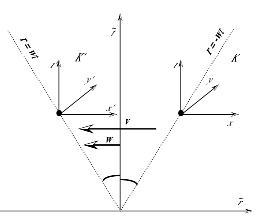
Figure 1: The physical meaning of symmetric velocity. Two inertial systems $K$ and $K^{\prime}$ with relative velocity $\mathbf{v}$ between them are viewed from the system connected to their center. In this system, $K$ and $K^{\prime}$ are each moving with velocity $\pm\mathbf{w}$.

Instead of $\mathbf{w_{s}}$, we shall find it more convenient to use the unit-free vector $\mathbf{w}=\mathbf{w_{s}}/c$, which we call the s-velocity. The relation of a velocity $\mathbf{v}$ to its corresponding s-velocity is

$$\mathbf{v}=\Phi(\mathbf{w})=\frac{2c\mathbf{w}}{1+|\mathbf{w}|^{2}},$$ (21)

where $\Phi$ denotes the function mapping the s-velocity $\mathbf{w}$ to its corresponding velocity $\mathbf{v}$. The s-velocity has some interesting and useful mathematical properties. The set of all three-dimensional relativistically admissible s-velocities forms a unit ball

$$D_{s}=\{\mathbf{w}\in R^{3}:\;|\mathbf{w}|<1\}.$$ (22)

Corresponding to the Einstein velocity addition equation, we may define an addition of s-velocities in $D_{s}$ such that

$$\Phi(\mathbf{b}\oplus_{s}\mathbf{w})=\Phi(\mathbf{b})\oplus_{E}\Phi(\mathbf{w}).$$ (23)

A straightforward calculation leads to the corresponding equation for s-velocity addition:

$$\mathbf{b}\oplus_{s}\mathbf{w}=\frac{(1+|\mathbf{w}|^{2}+2<\mathbf{b}\mid\mathbf{w}>)\mathbf{b}+(1-|\mathbf{b}|^{2})\mathbf{w}}{1+|\mathbf{b}|^{2}|\mathbf{w}|^{2}+2<\mathbf{b}\mid\mathbf{w}>}.$$ (24)

Equation (24) can be put into a more convenient form if, for any $\mathbf{b}\in D_{s}$, we define a map $\Psi_{\mathbf{b}}:D_{s}\to D_{s}$ by

$$\psi_{\mathbf{b}}(\mathbf{w})\equiv\mathbf{b}\oplus_{s}\mathbf{w}.$$ (25)

This map is an extension to $D_{s}\in R^{n}$ of the Möbius addition on the complex unit disc. It defines a conformal map on $D_{s}$. The motion of a charge in $\mathbf{E}\times\mathbf{B}$ fields is two-dimensional if the charge starts in the plane perpendicular to $\mathbf{B}$, and in this case Eq.(24) for s-velocity addition is somewhat simpler. By introducing a complex structure on the plane $\Pi$, which is perpendicular to $\mathbf{B}$, the disk $\Delta=D_{s}\cap\Pi$ can be identified as a unit disc $|z|<1$ called the Poincaré disc. In this case the s-velocity addition defined by Eq.(24) becomes

$$a\oplus_{s}w=\psi_{{a}}({w})=\frac{a+w}{1+\overline{a}w},$$ (26)

which is the well-known Möbius transformation of the unit disk.

By using the $s$ velocity we can rewrite [4],[9] the relativistic Lorentz force equation

$$\frac{d}{dt}(\gamma m\mathbf{v})=q({\bf E}+\mathbf{v}\times{\bf B})$$

as

$$\frac{m_{0}c}{q}\,\frac{d\mathbf{w}}{d\tau}=\left(\frac{1+|\mathbf{w}|^{2}}{2}\right){\bf{E}}+c\mathbf{w}\times{\bf{B}}-\mathbf{w}<\mathbf{w}|{\bf{E}}>,$$ (27)

which is the relativistic Lorentz force equation for the s-velocity $\mathbf{w}$ as a function of the proper time $\tau$.

We now use Eq.(27) to find the s-velocity of a charge $q$ in uniform, constant, and mutually perpendicular electric and magnetic fields. Since all of the terms on the right hand side of Eq. (27) are in the plane perpendicular to ${\mathbf{B}}$, if $\mathbf{w}\in\Pi$, therefore $d{\mathbf{w}}/{d\tau}$ is in the plane $\Pi$ perpendicular to ${\mathbf{B}}$. Consequently, if the initial s-velocity is in the plane perpendicular to ${\mathbf{B}}$, ${\mathbf{w}}$ will remain in the this plane and the motion will be two dimensional.

Working in Cartesian coordinates, we choose

$$\mathbf{E}=(0,E,0),\;\mathbf{B}=(0,0,B),\;\mbox{and}\;\mathbf{w}=(w_{1},w_{2},0).$$ (28)

By introducing a complex structure in $\Pi$ by denoting $w=w_{1}+iw_{2}$ the evolution equation Eq.(27) get the following simple form:

$$\frac{dw}{d\tau}=i\Omega\left(w^{2}-2\widetilde{B}w+1\right),$$ (29)

where

$$\Omega\equiv\frac{qE}{2m_{0}c}\;\;\mbox{and}\;\;\widetilde{B}\equiv\frac{cB}{E}.$$ (30)

The solution of Eq.(29) is unique for a given initial condition

$$w(0)=w_{0},$$ (31)

where the complex number $w_{0}$ represents the initial s-velocity $\mathbf{w}_{0}=\Phi^{-1}(\mathbf{v}_{0})$ of the charge.

Integrating Eq.(29) produces the equation

$$\int\frac{dw}{w^{2}-2\widetilde{B}w+1}=i\Omega\tau+C,$$ (32)

where the constant $C$ is determined from the initial condition (31). The way we evaluate this integral depends upon the sign of the discriminant $4\widetilde{B}^{2}-4$ associated with the denominator of the integrand. If we define

$$\Delta\equiv\widetilde{B}^{2}-1=\frac{(cB)^{2}-E^{2}}{E^{2}},$$ (33)

then the three cases $E<cB,E=cB\;\mbox{and}\;E>cB$ correspond to the cases $\Delta$ greater than zero, equal to zero, and less than zero.

Case 1 Consider first the case

$$\Delta=((cB)^{2}-{E}^{2})/{E}^{2})>0\Longleftrightarrow{E}<cB\;\mbox{and}\;\widetilde{B}>1.$$ (34)

The denominator of the integrand in (32) can be rewritten as

$$w^{2}-2\widetilde{B}w+1=(w-\alpha_{1})(w-\alpha_{2}),$$ (35)

where $\alpha_{1}$ and $\alpha_{2}$ are the real, positive roots

$$\alpha_{1}=\widetilde{B}-\sqrt{\widetilde{B}^{2}-1}\;\;\mbox{and}\;\;\alpha_{2}=\widetilde{B}+\sqrt{\widetilde{B}^{2}-1}.$$ (36)

and the solution become:

$$w(\tau)=\frac{\alpha_{1}+Ce^{-i\nu\tau}}{1+\alpha_{1}Ce^{-i\nu\tau}}=\alpha_{1}\oplus_{s}Ce^{-i\nu\tau},$$ (37)

where $\nu=2\sqrt{\Delta}\Omega$. This equation shows that in a system K’ moving with s-velocity $\alpha_{1}$ relative to the lab, the s-velocity of the charge corresponds to circular motion with initial s-velocity

$$C=\psi_{-\alpha_{1}}(w_{0}).$$ (38)

From Eqs.(21) and (36) it follows that the lab velocity corresponding to s-velocity $\alpha_{1}$ is

$$\frac{2c\alpha_{1}}{1+|\alpha_{1}|^{2}}=(E/B)\mathbf{i}=\mathbf{v}_{d}=v_{d}\mathbf{i},$$ (39)

which is the well-known $\mathbf{E}\times\mathbf{B}$ drift velocity. Applying the map $\Phi$ defined in Eq.(23) to both sides of (37), we get

$$\mathbf{v}(\tau)=\mathbf{v}_{d}\oplus_{E}e^{-i\nu\tau}\Phi(C).$$ (40)

Eq.(40) says that the total velocity of the charge, as a function of the proper time, is the sum of a constant drift velocity $\mathbf{v}_{d}=(E/B)\mathbf{i}$ and circular motion, as expected.

If $\mathbf{v}(0)=0$, then the $s$ velocity of the charge as a function of the proper time is ${\mathbf{b}}(\tau)=\alpha_{1}(1-\cos\nu\tau,-\sin\nu\tau),$ the velocity of the charge is

$$\mathbf{v}_{\mathbf{b}}(\tau)={v}_{d}(1-\cos\nu\tau,-\sin\nu\tau),$$

the position of the charge is

$$\mathbf{r}_{\mathbf{b}}(\tau)=\int_{0}^{\tau}\gamma\mathbf{v}(\tau^{\prime})\,d\tau^{\prime}=\frac{\gamma_{d}v_{d}}{\nu}\left(\gamma_{d}(\nu\tau-\sin{\nu\tau}),(\cos\nu\tau-1)\right)$$ (41)

and the lab time $t$ as a function of the proper time is

$$t_{\mathbf{b}}(\tau)=\int_{0}^{\tau}\gamma(\tau^{\prime})d\tau^{\prime}=\frac{\gamma_{d}^{2}}{\nu}\left(\nu\tau-\frac{v_{d}^{2}}{c^{2}}\sin{\nu\tau}\right),$$ (42)

where $\gamma_{d}=\gamma(\mathbf{v}_{d})$.

Case 2  Next consider the case $\Delta=((cB)^{2}-{E}^{2})/{E}^{2}=0\Longleftrightarrow{E}=c{B}\;\mbox{and}\;\widetilde{B}=1$. The denominator in the integrand of (32) is $w^{2}-2w+1=(w-1)^{2}$ and its solution is

$$w(\tau)=1-\frac{1}{i\Omega\tau+C}$$ (43)

with $C=-\frac{1}{w_{0}-1}.$

If the initial velocity is zero, $C=1$ the $s$ velocity of the charge as a function of the proper time is

$${\mathbf{b}}(\tau)=\frac{(\Omega^{2}\tau^{2},\Omega\tau)}{1+\Omega^{2}\tau^{2}},$$

the velocity of the charge

$$\mathbf{v}_{\mathbf{b}}(\tau)=\frac{2c(\Omega^{2}\tau^{2},\Omega\tau)}{1+2\Omega^{2}\tau^{2}},$$

the position of the charge is

$$\mathbf{r}_{\mathbf{b}}(\tau)=2c\left(\frac{\Omega^{2}\tau^{3}}{3},\frac{\Omega\tau^{2}}{2}\right)$$ (44)

and the lab time as a function of the proper time is

$$t_{\mathbf{b}}(\tau)=\int_{0}^{\tau}\gamma d\tau=\tau+\frac{2\Omega^{2}}{3}\tau^{3}.$$ (45)

Equations (44) and (45) give the complete solution for this case.

Case 3  Consider the case $\Delta=((cB)^{2}-E^{2})/{E}^{2}<0\;\Longleftrightarrow{E}>cB\;\mbox{or}\;\widetilde{B}<1$.

Just as in Case 1, we rewrite the denominator of the integrand in Eq. (32) as $w^{2}-2\widetilde{B}w+1=(w-\alpha_{1})(w-\alpha_{2}),$ where

$$\alpha_{1}=\widetilde{B}-i\delta\;\;\mbox{and}\;\;\alpha_{2}=\widetilde{B}+i\delta=\overline{\alpha}_{1}$$ (46)

and $\delta=\sqrt{1-\widetilde{B}^{2}}>0.$ By introducing

$$\nu=\left(\frac{q}{mc}\right)\sqrt{E^{2}-(cB)^{2}}.$$ (47)

and an s-velocity ${w}_{d}\equiv{\widetilde{B}}/\left({1+\delta}\right)$ we can write the solution as:

$$w(\tau)=w_{d}\oplus_{s}(i\tanh(\nu\tau)\oplus_{s}\widetilde{w}_{0}),$$ (48)

where $\widetilde{w}_{0}=\psi_{-w_{d}}(w_{0}).$

For the velocity of the charge we get

$$\mathbf{v}(\tau)=\mathbf{v}_{d}\oplus_{E}(c\tanh(2\nu\tau)\mathbf{j}\oplus\widetilde{\mathbf{v}}_{0}),$$ (49)

where $\mathbf{v}_{d}=(c^{2}B/E)\mathbf{i}$ is the drift velocity and $\widetilde{\mathbf{v}}_{0}$ is the initial velocity in the drift frame. From this it follows that for initial zero velocity, the velocity of the charge as a function of the proper time is

$$\mathbf{v}_{\mathbf{b}}(\tau)=\frac{\left(\gamma_{d}{v}_{d}(\cosh(\nu^{\prime}\tau)-1),c\sinh(\nu^{\prime}\tau)\right)}{\gamma_{d}\left(\cosh(\nu^{\prime}\tau)-{v_{d}^{2}}/{c^{2}}\right)},$$

its position

$$\mathbf{r}_{\mathbf{b}}(\tau)=\int_{0}^{\tau}\gamma\mathbf{v}(\tau^{\prime})\,d\tau^{\prime}=\frac{\gamma_{d}}{\nu^{\prime}}\left(\gamma_{d}v_{d}(\sinh(\nu^{\prime}\tau)-\nu^{\prime}\tau),c(\cosh(\nu^{\prime}\tau)-1)\right)$$ (50)

and the lab time $t$ as a function of the proper time is

$$t_{\mathbf{b}}(\tau)=\int_{0}^{\tau}\gamma(\tau^{\prime})d\tau^{\prime}=\gamma_{d}^{2}\left(\frac{\sinh(\nu^{\prime}\tau)}{\nu^{\prime}}-\frac{v_{d}^{2}}{c^{2}}\tau\right).$$ (51)

Equations (50) and (51) together give the complete solution for this case.

In all cases, for arbitrary initial velocity $\mathbf{v}_{0},$ the velocity of the charge at its proper time $\tau$ will be given by (see [4] p.87)

$$\mathbf{v}(\tau)=\varphi_{\mathbf{v}_{\mathbf{b}}(\tau)}(U_{\mathbf{b}}(\tau)\mathbf{v}_{0}),$$ (52)

where $\varphi$ is defined by (11), $\mathbf{v}_{\mathbf{b}}$ was defined in each case separately and $U_{\mathbf{b}}(\tau)$ is a rotation in the plane $x,y$ given by the complex number

$$\frac{1-\widetilde{B}\mathbf{b}(\tau)}{1-\widetilde{B}\overline{\mathbf{b}}(\tau)}.$$ (53)

This mean that for the electromagnetic field $\mathbf{E},\mathbf{B}$ in an inertial system $K$, with $\mathbf{E}$ perpendicular to $\mathbf{B}$, in the frame $\tilde{K}$ boosted with $\mathbf{v}_{\mathbf{b}}(\tau)$ and rotated with $U_{\mathbf{b}}(\tau)$ with respect to our inertial system all charged particles of the same mass and charge will continue to move with their initial velocity. This mean that with respect to system $\tilde{K}$ the motion of charged particles is not affected by the electromagnetic field. This is similar to Equivalence Principle for the gravitational field.

4 Space-time transformations from an inertial system to a uniformly accelerated and rotating system assuming the clock-hypothesis

Results of the previous section could be applied to find the space-time transformations between an inertial system $K$ and a uniformly accelerated and rotating system $\tilde{K}$. The motion of a charge in a constant uniform electric field is considered as a uniformly accelerated motion, while the motion in a magnetic field is considered as constant rotation. Thus, constant uniform acceleration and rotation may be described by the action of a constant electromagnetic field $\mathbf{E},\mathbf{B}$ on charged particles. In this section we will deal only with uniformly accelerated and rotating motion for which the axes of rotation is perpendicular to direction of the acceleration. This corresponds to perpendicularity of the corresponding electric and magnetic fields.

Let $K$ denote an inertial system with with origin $O$ and space-time coordinates $\left(\begin{array}[]{c}t\\ \mathbf{r}\end{array}\right).$ Let a system $\tilde{K}$ with origin $\tilde{O}$ move with constant uniform acceleration and rotation is described by the action of a constant electromagnetic field $\mathbf{E},\mathbf{B}$, with $\mathbf{E}$ perpendicular to $\mathbf{B}$, on charged particles. Without loss of generality we may assume that $\mathbf{E},$ generating the acceleration, is in the direction of the $y$-axis, i.e. $\mathbf{E}=(0,E,0)$ and $\mathbf{B},$ generating the rotation around the $z$-axis, i.e. $\mathbf{B}=(0,0,B)$. We assume that the clocks and the space axes at time $t=0$ in systems $K$ and $\tilde{K}$ were synchronized. A charge positioned at common origin of the systems at time $t=0$ remains at $\tilde{O}$ for any time $t>0$. Thus, by the results of the previous section, the world line of this charge or of $\tilde{O}$ is $\left(\begin{array}[]{c}t_{\mathbf{b}}(\tau)\\ \mathbf{r}_{\mathbf{b}}(\tau)\end{array}\right),$ where $\tau$ denote the proper time of the charge and $t_{\mathbf{b}}(\tau)$ and $\mathbf{r}_{\mathbf{b}}(\tau)$ are defined by the appropriate formulas for each of the 3 cases.

For a given time $t_{0}$ we denote by $K^{\prime}$ an inertial system with origin $O^{\prime}$ which is positioned and have the same velocity as $\tilde{O}$ at time $t_{0}$ and have common space axes at time $t_{0}$ with system $\tilde{K}$. The system $K^{\prime}$ is called a comoving system to system $\tilde{K}$ at time $t_{0}$. The Clock hypothesis state that the time in $\tilde{K}$ is the same as the time in $K^{\prime}$. As we will see later, the Clock hypothesis imply that the space coordinates in $\tilde{K}$ and $K^{\prime}$ are the same. Thus, the space-time transformations from $K$ to $\tilde{K}$ coincide with the transformations between $K$ and $K^{\prime}.$

Consider an event that occurs at $\left(\begin{array}[]{c}\tilde{t}\\ \mathbf{\tilde{r}}\end{array}\right)$ in the uniformly accelerated and rotated system $\tilde{K}$.Let $K^{\prime}$ be the inertial system comoving to $\tilde{K}$ at time $t_{0}=\tilde{t}$. By the Clock hypothesis this event has the same space-time coordinates in $K^{\prime}$. The position of the origins $O^{\prime}$ and $\tilde{O}$ is $\mathbf{r}_{\mathbf{b}}(\tilde{t})$ in $K$ and the time at the clock at $\tilde{O}$ shows time $\tilde{t}$ which correspond to $t_{\mathbf{b}}(\tilde{t})$ in system $K$. Moreover the space axes in $K$ are rotated with respect to the space axes in $K^{\prime}$ by $U_{\mathbf{b}}(\tilde{t}),$ defined by (53). The relative velocity of $K^{\prime}$ and $K$ is given by $\mathbf{v}_{\mathbf{b}}(\tilde{t}),$ defined by the appropriate formulas for each of the 3 cases. We use a modification of the space-time Lorentz transformations (2) between two inertial systems which were not synchronized at time $t=0$ for the space-time transformation from $K^{\prime}$ to $K$. This imply that the space-time coordinates of the considered event in $K$ are

$$\left(\begin{array}[]{c}{t}\\ \mathbf{{r}}\end{array}\right)=\left(\begin{array}[]{c}t_{\mathbf{b}}(\tilde{t})\\ \mathbf{r}_{\mathbf{b}}(\tilde{t})\end{array}\right)+\left(\begin{array}[]{c}\gamma c^{-2}\langle\mathbf{v}_{\mathbf{b}}(\tilde{t})|U_{\mathbf{b}}(\tilde{t})\mathbf{\tilde{r}}\rangle\\ (\gamma P_{\mathbf{v}_{\mathbf{b}}(\tilde{t})}+(I-P_{\mathbf{v}_{\mathbf{b}}(\tilde{t})}))U_{\mathbf{b}}(\tilde{t})\mathbf{\tilde{r}}\end{array}\right),$$ (54)

where $\gamma=\gamma(\mathbf{v}_{\mathbf{b}}(\tilde{t})).$

If we do not assume the validity of the Clock Hypothesis, the above transformations will hold with respect to the comoving frame $K^{\prime}$ only. Thus, in order to describe general space-time transformations between two systems uniformly accelerated with respect to the same inertial system, it is enough to describe such transformations only for systems which at some initial time have the same velocity, which were called comoving systems. For example, systems $K^{\prime},$ which is an inertial system, could be considered as moving with uniform zero acceleration with respect to the inertial system $K$ and system $\tilde{K}$, which is uniformly accelerated with respect to the inertial system $K$ are comoving with respect to $t_{0}$. Thus, they provide an example of uniformly accelerated comoving systems. Such transformation are described in [8].

References

• [1] W. E. Baylis, Electrodynamics, A Modern Geometric Approach, Progress in Physics 17, Birkhäuser, Boston, 1999.
• [2] M. Born, Einstein’s Theory of Relativity , Dover Publications, New York, 1965.
• [3] C. X. Chen, G. Papini, N. Mobed, G. Lambiaise, G. Scarpetta, Nuovo Cimento 114B (1999) 1335.
• [4] Y. Friedman, Homogeneous balls and their Physical Applications, Progress in Mathematical Physics 40, (Birkhäuser, Boston, 2004.
• [5] Y. Friedman, Yu. Gofman, Why Does the Geometric Product Simplify the Equations of Physics?, International Journal of Theoretical Physics, 41 (2002), 1861–1875.
• [6] Y. Friedman, Yu. Gofman, Relativistic Linear Spacetime Transformations Based on Symmetry, Foundations of Physics, 32 (2002), 1717–1736.
• [7] Y. Friedman, Yu. Gofman, in Gravitation, Cosmology and Relativistic Astrophysics, A Collection of Papers (Kharkov National University, Kharkov, Ukraine, 2004), 102.
• [8] Y. Friedman, Yu. Gofman, Kinematic relations between relativistically accelerated systems in flat space-time based on symmetry, arxiv/gr-qc/0509004.
• [9] Y. Friedman, M.Semon, Relativistic acceleration of charged particles in uniform and mutually perpendicular electric and magnetic fields as viewed in the laboratory frame, Phys. Rev. E 72 (2005), 026603.
• [10] G. Lambiaise, G. Papini, G. Scarpetta, Nuovo Cimnto 114 (1999) 189.
• [11] W. Pauli, Theory of Relativity (Pergamon Press, London, 1958).
• [12] F. P. Schuller, Ann. Phys. 299 (2002) 174.
• [13] G. Scarpetta, Lett. Nuovo Cimento 41 (1984) 51.
• [14] S. Takeuchi, Phys. Rev. E66, 37402-1 (2002).