Abstract

In this paper we explicitly work out the secular perturbations induced on all the Keplerian orbital elements of a test body to order $\mathcal{O}(e^{2})$ in the eccentricity $e$ by the weak-field long-range modifications of the usual Newton-Einstein gravity due to the Dvali-Gabadadze-Porrati (DGP) braneworld model. Both the Gauss and the Lagrange perturbative schemes are used. It turns out that the argument of pericentre $\omega$ and the mean anomaly $\mathcal{M}$ are affected by secular rates which depend on the orbital eccentricity via $\mathcal{O}(e^{2})$ terms, but are independent of the semimajor axis of the orbit of the test particle. For circular orbits the Lue-Starkman (LS) effect on the pericentre is obtained. Some observational consequences are discussed for the Solar System planetary mean longitudes $\lambda$ which would undergo a $1.2\cdot 10^{-3}$ arcseconds per century braneworld secular precession. According to recent data analysis over 92 years for the EPM2004 ephemerides, the 1-sigma formal accuracy in determining the Martian mean longitude amounts to $3\cdot 10^{-3}$ milliarcseconds, while the braneworld effect over the same time span would be $1.159$ milliarcseconds. The major limiting factor is the $2.6\cdot 10^{-3}$ arcseconds per century systematic error due to the mismodelling in the Keplerian mean motion of Mars. A suitable linear combination of the mean longitudes of Mars and Venus may overcome this problem. The formal, 1-sigma obtainable observational accuracy would be $\sim 7\%$. The systematic error due to the present-day uncertainties in the solar quadrupole mass moment $J_{2}$, the Keplerian mean motions, the general relativistic Schwarzschild field and the asteroid ring would amount to some tens of percent.

1 Introduction

Recently, a braneworld scenario which yields, among other things, long-range modifications of the Newton-Einstein gravity has been put forth by Dvali, Gabadadze and Porrati (DGP) [1, 2]. In such model, which encompasses an extra flat spatial dimension, there is a free crossover parameter $r_{0}$, fixed by observations to a value $\sim 5$ Gpc, beyond which traditional gravity suffers strong modifications yielding to cosmological consequences which would yield an alternative to the dark energy in order to explain the observed acceleration of the Universe. The consistency and stability of the DGP model have recently been discussed in [3].

Interestingly, for $R_{\rm g}<<r<<r_{0}$, where $R_{\rm g}=2GM/c^{2}$ is the usual Schwarzschild radius for a gravitating body of mass $M$, there are also small modifications to the usual Newton-Einstein gravity which could be detectable in a near future. Indeed, Lue and Starkman (LS) derived in [4] an extra-pericentre advance for the orbital motion of a test particle assumed to be nearly circular. Its magnitude is $\sim 4\cdot 10^{-4}$ arcseconds per century (^′′ cy^-1 in the following). In [4] it has been shown that the sign of such an effect is related to the cosmological expansion phases allowed in this model: the Friedmann-Lemaître-Robertson-Walker (FLRW) phase and the self-accelerating phase. The LS precession is an universal feature of the orbital dynamics of a test particle because, in this approximation, it is independent of its orbital parameters.

Since the present-day accuracy in measuring the non-Newtonian perihelion rate of Mars amounts to $\sim 10^{-4}$ ^′′ cy^-1 (E.V. Pitjeva, private communication 2004), the possibility of measuring such an effect in the Solar System scenario from the planetary motion data analysis seems to be very appealing. It has been investigated with some details in [6] where a suitable linear combination of the perihelia of some inner planets has been considered.

In this paper we work out the secular effects of the DGP model on all the Keplerian orbital elements of a test body to order $\mathcal{O}(e^{2})$ in the eccentricity $e$ with the Gauss and Lagrange perturbative schemes. Possible observational implications are worked out.

2 The orbital effects

In this Section we will work out the secular effects of the DGP gravity on the Keplerian orbital elements of the orbit of a test body which is depicted in Figure 1.

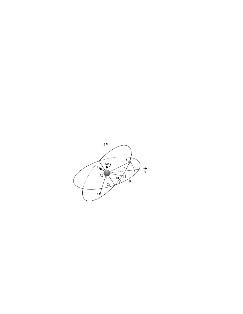
Figure 1: Orbital geometry for a motion around a central mass. Here $L$ denotes the orbital angular momentum of the particle of mass $m$, $J$ is the proper angular momentum of the central mass $M$, $\Pi$ denotes the pericentre position, $f$ is the true anomaly of $m$, which is counted from $\Pi$, $\Omega$, $\omega$ and $i$ are the longitude of the ascending node, the argument of pericentre and the inclination of the orbit with respect to the inertial frame $\{x,y,z\}$ and the azimuthal angle $\phi$ is the right ascension counted from the $x$ axis. When orbits with small inclinations are considered, the longitude of pericentre $\varpi=\Omega+\omega$ is used.

From the metric for a static, spherical source in a cosmological de Sitter background [4]

$$(ds)^{2}=N^{2}(r,w)(cdt)^{2}-A^{2}(r,w)(dr)^{2}-B^{2}(r,w)[(d\theta)^{2}+\sin^{2}\theta(d\phi)^{2}]-(dw)^{2},$$ (1)

where $w$ is the fourth spatial coordinate, and

$$N\sim 1-{R_{\rm g}\over 2r}\pm\sqrt{{rR_{\rm g}\over 2r_{0}^{2}}},$$ (2)

the following Lagrangian can be obtained for a spherically symmetric matter source located on the brane around the origin ($r=w=0$)

$$\mathcal{L}_{\rm DGP}={m\over 2}\left[\left(1-{R_{g}\over 2r}\pm\sqrt{{R_{\rm g}r\over 2r_{0}^{2}}}\right)^{2}c^{2}-(\dot{x})^{2}-(\dot{y})^{2}-(\dot{z})^{2}\right].$$ (3)

2.1 The Gauss perturbative scheme

From

$${d\over dt}\left({{\partial{\mathcal{L}}\over\partial{{\boldsymbol{v}}}}}\right)-{\partial{\mathcal{L}}\over\partial{\boldsymbol{r}}}=0$$ (4)

the resulting braneworld acceleration is

$$\boldsymbol{A}_{\rm DGP}=\mp\left({c\over 2r_{0}}\right)\sqrt{{GM\over r}}\boldsymbol{\hat{r}},$$ (5)

where $\boldsymbol{\hat{r}}$ is the unit vector in the radial direction. The term (5) can be regarded as a small perturbation whose effects on the Keplerian orbital elements of a test particle can be straightforwardly worked out, e.g., in the Gauss perturbative scheme (e.g. [8]). Note that (5) is purely radial.

The Gauss rate equations for the semimajor axis $a$, the eccentricity $e$, the inclination $i$, the longitude of the ascending node $\Omega$, the argument of pericentre $\omega$ and the mean anomaly $\mathcal{M}$ of a test particle are

$$\frac{{{d}}{a}}{{{d}}{t}} = {2\over n\sqrt{1-e^{2}}}\left[A_{R}e\sin f+A_{T}\left({p\over r}\right)\right],$$ (6)

$$\frac{{{d}}{e}}{{{d}}{t}} = {\sqrt{1-e^{2}}\over na}\left\{A_{R}\sin f+A_{T}\left[\cos f+{1\over e}\left(1-{r\over a}\right)\right]\right\},$$ (7)

$$\frac{{{d}}{i}}{{{d}}{t}} = {1\over na\sqrt{1-e^{2}}}A_{N}\left({r\over a}\right)\cos(\omega+f),$$ (8)

$$\frac{{{d}}{\Omega}}{{{d}}{t}} = {1\over na\sin i\sqrt{1-e^{2}}}A_{N}\left({r\over a}\right)\sin(\omega+f),$$ (9)

$$\frac{{{d}}{\omega}}{{{d}}{t}} = -\cos i\frac{{{d}}{\Omega}}{{{d}}{t}}+{\sqrt{1-e^{2}}\over nae}\left[-A_{R}\cos f+A_{T}\left(1+{r\over p}\right)\sin f\right],$$ (10)

$$\frac{{{d}}{\mathcal{M}}}{{{d}}{t}} = n-{2\over na}A_{R}{r\over a}-\sqrt{1-e^{2}}\left(\frac{{{d}}{\omega}}{{{d}}{t}}+\cos i\frac{{{d}}{\Omega}}{{{d}}{t}}\right),$$ (11)

in which $n\equiv 2\pi/P=\sqrt{GM/a^{3}}$ is the Keplerian mean motion, $P$ is the test particle’s orbital period, $f$ is the true anomaly counted from the pericentre, $p=a(1-e^{2})$ is the semilactus rectum of the Keplerian ellipse, $A_{R},\ A_{T},\ A_{N}$ are the in-plane radial, transverse and the out-of-plane components of the perturbing acceleration, respectively, which have to be evaluated on the unperturbed Keplerian ellipse

$$r={a(1-e^{2})\over 1+e\cos f}.$$ (12)

The secular effects can be obtained by averaging over one orbital period the right-hand-sides of (6)-(11) evaluated on (12). The average is performed by using

$${dt\over P}={(1-e^{2})^{3/2}df\over 2\pi(1+e\cos f)^{2}}$$ (13)

and integrating from 0 to $2\pi$. Since the perturbing acceleration is entirely radial, from (8)-(9) it is straightforward to note that there are no perturbations in the inclination and the node. In regard to the other elements, the following expansions have been performed

$$(1+e\cos f)^{-3/2} \sim 1-{3\over 2}e\cos f+{15\over 8}e^{2}\cos^{2}f-{35\over 16}e^{3}\cos^{3}f,$$ (14)

$$(1+e\cos f)^{-5/2} \sim 1-{5\over 2}e\cos f+{35\over 8}e^{2}\cos^{2}f.$$ (15)

The expansion (14) has been used for the semimajor axis, the eccentricity and the pericentre, while the expansion (15) has been used for the mean anomaly.

It turns out that only the pericentre and the mean anomaly undergo secular effects which are, to order $\mathcal{O}(e^{2})$

$$\frac{{{d}}{\omega}}{{{d}}{t}} \sim \mp{3c\over 8r_{0}}\left(1-{13\over 32}e^{2}\right),$$ (16)

$$\frac{{{d}}{\mathcal{M}}}{{{d}}{t}} \sim \pm{11c\over 8r_{0}}\left(1-{39\over 352}e^{2}\right).$$ (17)

For $e\rightarrow 0$ (16) reduces to the result by Lue and Starkman for circular orbits [4].

2.2 The Lagrangian perturbative scheme

The Lagrange planetary equations for the rates of change of the Keplerian orbital elements are (e.g. [9])

$$\frac{{{d}}{a}}{{{d}}{t}} = {2\over na}\ {\partial{\mathcal{R}}\over\partial{\mathcal{M}}},$$ (18)

$$\frac{{{d}}{e}}{{{d}}{t}} = {(1-e^{2})\over na^{2}e}\ {\partial{\mathcal{R}}\over\partial{\mathcal{M}}}-{\sqrt{1-e^{2}}\over na^{2}e}\ {\partial{\mathcal{R}}\over\partial{\omega}},$$ (19)

$$\frac{{{d}}{i}}{{{d}}{t}} = \cos{i}{1\over na^{2}\sqrt{1-e^{2}}\sin{i}}\ {\partial{\mathcal{R}}\over\partial{\omega}}-{1\over na^{2}\sqrt{1-e^{2}}\sin{i}}\ {\partial{\mathcal{R}}\over\partial{\Omega}},$$ (20)

$$\frac{{{d}}{\Omega}}{{{d}}{t}} = {1\over na^{2}\sqrt{1-e^{2}}\sin{i}}\ {\partial{\mathcal{R}}\over\partial{i}},$$ (21)

$$\frac{{{d}}{\omega}}{{{d}}{t}} = -\cos{i}{1\over na^{2}\sqrt{1-e^{2}}\sin{i}}\ {\partial{\mathcal{R}}\over\partial{i}}+{\sqrt{1-e^{2}}\over na^{2}e}\ {\partial{\mathcal{R}}\over\partial{e}},$$ (22)

$$\frac{{{d}}{\mathcal{M}}}{{{d}}{t}} = n-{(1-e^{2})\over na^{2}e}\ {\partial{\mathcal{R}}\over\partial{e}}-{2\over na}\ {\partial{\mathcal{R}}\over\partial{a}},$$ (23)

where $\mathcal{R}$ is the perturbing function which accounts for all the departures of the gravitational potential from the Newtonian monopole term. Such a perturbing scheme was applied for the first time to post-Newtonian motions by Rubincam [10]. In the case of the DGP braneworld theory from $\mathcal{H}=\boldsymbol{p}\cdot\boldsymbol{v}-\mathcal{L}$, $\boldsymbol{p}=\partial\mathcal{L}/\partial\boldsymbol{v}$, and (3) it can be obtained

$$\mathcal{R}_{\rm DGP}=\mp{c\over r_{0}}\sqrt{GMr}.$$ (24)

The DGP perturbing function (24) has to be evaluated on the unperturbed Keplerian ellipse (12) and averaged over one orbital revolution by means of (13) in order to obtain the secular effects. From

$$(1+e\cos f)^{-5/2}\sim 1-{5\over 2}e\cos f+{35\over 8}e^{2}\cos^{2}f-{105\over 16}e^{3}\cos^{3}f+{1155\over 128}e^{4}\cos^{4}f,$$ (25)

one obtains

$$\left\langle\mathcal{R}\right\rangle\sim\mp{c\sqrt{GMa}\over r_{0}}\left(1+{3\over 16}e^{2}+{9\over 1024}e^{4}\right).$$ (26)

Since

$${\partial{\left\langle\mathcal{R}\right\rangle}\over\partial{\mathcal{M}}}={\partial{\left\langle\mathcal{R}\right\rangle}\over\partial{\Omega}}={\partial{\left\langle\mathcal{R}\right\rangle}\over\partial{\omega}}={\partial{\left\langle\mathcal{R}\right\rangle}\over\partial{i}}=0,$$ (27)

is it straightforward to obtain

$$\frac{{{d}}{a}}{{{d}}{t}}=\frac{{{d}}{e}}{{{d}}{t}}=\frac{{{d}}{i}}{{{d}}{t}}=\frac{{{d}}{\Omega}}{{{d}}{t}}=0.$$ (28)

The situation is different for the pericentre and the mean anomaly. Indeed,

$${\partial{\left\langle\mathcal{R}\right\rangle}\over\partial{e}} = \mp{3ec\sqrt{GMa}\over 8r_{0}}\left(1+{3\over 32}e^{2}\right),$$ (29)

$${\partial{\left\langle\mathcal{R}\right\rangle}\over\partial{a}} = \mp{c\over 2r_{0}}\sqrt{{GM\over a}}\left(1+{3\over 16}e^{2}+{9\over 1024}e^{4}\right).$$ (30)

As a consequence,

$$\frac{{{d}}{\omega}}{{{d}}{t}} \sim \mp{3c\over 8r_{0}}\left(1-{13\over 32}e^{2}\right),$$ (31)

$$\frac{{{d}}{\mathcal{M}}}{{{d}}{t}} \sim \pm{11c\over 8r_{0}}\left(1-{39\over 352}e^{2}\right).$$ (32)

Note that (31)-(32) are identical to (16)-(17) obtained in Section 2.1.

3 The possible use of the planetary mean longitudes

In [6] only the use of the planetary perihelia has been examined. First, preliminary observational tests are discussed in [7].

The fact that also the mean anomaly is affected by the DGP gravity with a relatively large effect suggests to examine the possibility of using the planetary mean longitudes $\lambda=\omega+\Omega+\mathcal{M}$.

3.1 The observational sensitivity

The sizes of the DGP secular precessions and of many Newtonian and Einsteinian competing secular precessions of the mean longitudes of the Solar System planets are reported in Table 1.

Table 1: Nominal values, in ^′′ cy^-1, of the secular precessions induced on the planetary mean longitudes $\lambda$ by the DGP gravity and by some of the competing Newtonian and Einsteinian gravitational perturbations. For a given planet, the precession labelled with Numerical includes all the numerically integrated perturbing effects of the dynamical force models used at JPL for the DE200 ephemerides. E.g., it also comprises the classical N- body interactions, including the Keplerian mean motion $n$. For the numerically integrated planetary precessions see http://ssd.jpl.nasa.gov/elem$\_$planets.html$\#$rates. The effect labelled with GE is due to the post-Newtonian general relativistic gravitoelectric Schwarzschild component of the solar gravitational field, that labelled with $J_{2}$ is due to the classical effect of the Sun’s quadrupole mass moment $J_{2}$ and that labelled with LT is due to the post-Newtonian general relativistic gravitomagnetic Lense-Thirring [12] component of the solar gravitational field (not included in the force models adopted by JPL). For $J_{2}$ the value $1.9\cdot 10^{-7}$ has been adopted [11]. For the Sun’s proper angular momentum $J$, which is the source of the gravitomagnetic field, the value $1.9\cdot 10^{41}$ kg m² s^-1 [13] has been adopted.

Planet	DGP	Numerical	GE	$J_{2}$	LT
Mercury	$1.2\cdot 10^{-3}$	$5.381016282\cdot 10^{8}$	$-8.48\cdot 10^{1}$	$4.7\cdot 10^{-2}$	$-2\cdot 10^{-3}$
Venus	$1.2\cdot 10^{-3}$	$2.106641360\cdot 10^{8}$	$-1.72\cdot 10^{1}$	$5\cdot 10^{-3}$	$-3\cdot 10^{-4}$
Earth	$1.2\cdot 10^{-3}$	$1.295977406\cdot 10^{8}$	$-7.6$	$1.6\cdot 10^{-3}$	$-1\cdot 10^{-4}$
Mars	$1.2\cdot 10^{-3}$	$6.89051037\cdot 10^{7}$	$-2.6$	$3\cdot 10^{-4}$	$-3\cdot 10^{-5}$
Jupiter	$1.2\cdot 10^{-3}$	$1.09250783\cdot 10^{7}$	$-1\cdot 10^{-1}$	$5\cdot 10^{-6}$	$-7\cdot 10^{-7}$
Saturn	$1.2\cdot 10^{-3}$	$4.4010529\cdot 10^{6}$	$-2\cdot 10^{-2}$	$6\cdot 10^{-7}$	$-1\cdot 10^{-7}$
Uranus	$1.2\cdot 10^{-3}$	$1.5425477\cdot 10^{6}$	$-4\cdot 10^{-3}$	$5\cdot 10^{-8}$	$-1\cdot 10^{-8}$
Neptune	$1.2\cdot 10^{-3}$	$7.864492\cdot 10^{5}$	$-1\cdot 10^{-3}$	$1\cdot 10^{-8}$	$-5\cdot 10^{-9}$

It can be noted that the DGP secular precessions amount to $1.2\cdot 10^{-3}$ ^′′ cy^-1 for all the planets: the corrections due to the eccentricities are very small amounting to almost $10^{-5}$ ^′′ cy^-1. In regard to the observational sensitivity, in Table 2, retrieved from Table 4 of [11], the most recent results for the EPM2004 ephemerides are presented.

Table 2: Formal standard deviations, in milliarcseconds (mas), of the planetary mean longitudes as from Table 4 of [11] for the EPM2004 ephemerides. Note that realistic errors may be an order of magnitude larger. About 300000 position observations (1911-2003) of different types (optical, radar, spacecraft, LLR) have been used. The braneworld shift for $\lambda$ amounts to 1.159 mas over a 92-years time span.

Mercury	Venus	Mars	Jupiter	Saturn	Uranus	Neptune
$3.75\cdot 10^{-1}$	$1.87\cdot 10^{-1}$	$3\cdot 10^{-3}$	1.109	3.474	8.818	$3.5163\cdot 10^{1}$

They are based on the processing of a vast amount of data of different kinds (optical, radar, spacecraft, LLR) ranging from 1911 to 2003. It can be noted that Mars is the best candidate for extracting the DGP effect because the formal standard deviation in $\lambda_{\rm Mars}$ amounts to $3\cdot 10^{-3}$ milliarcseconds (mas) only while the braneworld shift for the same time span is 1.159 mas.

4 Some systematic errors

In this Section we will examine various competing classical and general relativistic effects which would act as sources of systematic errors in order to see if it is possible to use only the Martian mean longitude for the proposed test.

4.1 The impact of the solar quadrupole mass moment and of the Einstein gravitoelectric force

In regard to the systematic errors which would induced by the other Newtonian and Einsteinian competing effects, the solar quadrupole mass moment $J_{2}$ is presently known with a 15$\%$ accuracy (Table 7 of [11]), so that the mismodelled part of its secular precession would be two orders of magnitude smaller than the effect of interest.

More important would be the impact of the Einsteinian gravitoelectric precession. Indeed, the general relativistic perihelion precession has been measured to a $10^{-4}$ relative accuracy via the PPN parameters $\beta$ and $\gamma$ (Table 8 of [11]): assuming that it would also hold for $\lambda$, this would yield a $2\cdot 10^{-4}$ ^′′ cy^-1 mismodelled effect. However, it should be noted that these are merely the formal 1-sigma errors: realistic bounds might be one order of magnitude larger.

4.2 The N-body perturbations

The mean longitude can be written as $\lambda=nt+\epsilon,$ so that [15]

$$\frac{{{d}}{\lambda}}{{{d}}{t}}=n+\frac{{{d}}{\epsilon^{\ast}}}{{{d}}{t}}\equiv n+\frac{{{d}}{n}}{{{d}}{t}}t+\frac{{{d}}{\epsilon}}{{{d}}{t}},$$ (33)

where

$$\frac{{{d}}{\epsilon}}{{{d}}{t}}=-{2\over na}{\partial{\mathcal{R}}\over\partial{a}}+{\sqrt{1-e^{2}}(1-\sqrt{1-e^{2}})\over na^{2}e}{\partial{\mathcal{R}}\over\partial{e}}+{\tan(i/2)\over na^{2}\sqrt{1-e^{2}}}{\partial{\mathcal{R}}\over\partial{i}}.$$ (34)

4.2.1 The direct and indirect effects on the Keplerian mean motion due to the other planets and the asteroids

In regard to the Keplerian mean motion, it turns out to be the major limiting factor. Indeed, the uncertainty in the solar $GM$ $\sigma_{GM_{\odot}}=8\cdot 10^{9}$ m³ s^-2 (Table 1 of [14]) yields $\sigma_{n_{\rm Mars}}=2.6\cdot 10^{-3}$ ^′′ cy^-1. However, if we adopt the position of keeping fixed the solar $GM$, the formal 1-sigma error due to the semimajor axis $\sigma_{a_{\rm Mars}}=6.57\cdot 10^{-1}$ m (Table 4 of [11]) only reduces to $\sigma_{n_{\rm Mars}}=3\cdot 10^{-4}$ ^′′ cy^-1.

Another source of potential bias is represented by the indirect perturbations on the Keplerian mean motion induced by the variations in the semimajor axis

$$\Delta n\equiv\frac{{{d}}{n}}{{{d}}{t}}t=-{3\over 2}{n\over a}\frac{{{d}}{a}}{{{d}}{t}}t=-{3\over a^{2}}{\partial{\langle\mathcal{R}\rangle}\over\partial{\lambda}}t.$$ (35)

According to [15], there are no secular effects on the semimajor axis: instead, the so called resonant perturbations, affect this Keplerian orbital element. They are induced by those terms in the expansion of the N-body disturbing function which retain the mean longitudes of the perturbed and the perturbing bodies. Such kind of harmonic perturbations, due to the asteroids for Mars, are potentially very insidious because they may have large amplitudes and extremely long periods. This topic has been treated in [16]. Table IV of [16] lists the most important of such perturbations. The nominal amplitudes of the perturbations induced, e.g., by (1) Ceres, (2) Pallas, (4) Vesta and (7) Iris are $4.7\cdot 10^{-2}$ ^′′ cy^-1, $1.2\cdot 10^{-2}$ ^′′ cy^-1, $5.7\cdot 10^{-2}$ ^′′ cy^-1 and $5\cdot 10^{-3}$ ^′′ cy^-1, respectively. According to the results of Table 6 of [11], their mismodelled parts amount to, $7\cdot 10^{-5}$ ^′′ cy^-1, $3\cdot 10^{-5}$ ^′′ cy^-1, $4\cdot 10^{-5}$ ^′′ cy^-1 and $8\cdot 10^{-5}$ ^′′ cy^-1, respectively. It must also be noted that the integrated shift of $\Delta n$ grows quadratically in time.

4.2.2 The perturbations on the mean longitude due to the other planets and the asteroid ring

Here we will deal with $d\epsilon/dt$ which is responsible for the secular perturbations on $\lambda$.

The Newtonian secular perturbations induced on the Mars mean longitude by the other planets of the Solar System are of the order of $10^{3}$ ^′′ cy^-1. The major source of uncertainty is represented by the $GM$ of the perturbing bodies among which Jupiter plays a dominant role, especially for Mars. According to [17], the Jovian $GM$ is known with a relative accuracy of $10^{-8}$; this would imply for the red planet a mismodelled precession induced by Jupiter of the order of $10^{-5}$ ^′′ cy^-1. The $GM$ of Saturn is known with a $1\cdot 10^{-6}$ relative accuracy [18]. However, the ratio of the secular precession induced on the Martian Keplerian elements by Saturn to that induced on the Mars perihelion by Jupiter is proportional to $(M_{\rm Sat}/M_{\rm Jup})(a_{\rm Jup}/a_{\rm Sat})^{3}\sim 5\cdot 10^{-2}$. This would assure that also the effect of Saturn is of the order of $10^{-5}$ ^′′ cy^-1. The situation with the precessions induced by Uranus and Neptune is even more favorable. Indeed, for Uranus $(M_{\rm Ura}/M_{\rm Jup})(a_{\rm Jup}/a_{\rm Ura})^{3}\sim 1\cdot 10^{-3}$ and the relative uncertainty in the uranian $GM$ is $2\cdot 10^{-6}$ [19]. For Neptune $(M_{\rm Nep}/M_{\rm Jup})(a_{\rm Jup}/a_{\rm Nep})^{\sim}3\cdot 10^{-4}$ and $\sigma_{GM}/GM=2\cdot 10^{-6}$ [20].

A source on potentially non-negligible perturbations on the Martian mean longitude is the asteroid ring, i.e. the ensemble of the minor asteroids whose impact can be modelled as due to a solid ring in the ecliptic plane [21]. The perturbations due to it can be worked out, e.g., with the Lagrangian approach and the disturbing function of the Appendix of [21]. By using the values of [11] for the ring’s radius and mass it turns out that the secular perturbation on $\dot{\lambda}_{\rm Mars}$ amounts to $-3.4\cdot 10^{-3}$ ^′′ cy^-1, with an uncertainty of $3\cdot 10^{-4}$ ^′′ cy^-1.

4.3 The total systematic error on the mean longitude of Mars

In Table 3 we summarize the various systematic errors affecting the mean longitude of Mars.

Table 3: Sources of systematic errors, in ^′′ cy^-1, affecting the mean longitude of Mars. The reported figures are at 1-sigma level. The total effect, obtained by summing up the various errors, is more than 90$\%$ of the braneworld signature.

Source of systematic error	Mismodelled amplitude (′′ cy-1)
Keplerian mean motion	$3\cdot 10^{-4}$
Asteroid ring	$3\cdot 10^{-4}$
Schwarzschild GE field	$2\cdot 10^{-4}$
(7) Iris	$8\cdot 10^{-5}$
(1) Ceres	$7\cdot 10^{-5}$
Solar $J_{2}$	$4.5\cdot 10^{-5}$
(4) Vesta	$4\cdot 10^{-5}$
(2) Pallas	$3\cdot 10^{-5}$
Lense-Thirring GM field (assumed unmodelled)	$3\cdot 10^{-5}$
Total	$1.1\cdot 10^{-3}$

It turns out that it is impossible to only analyze the mean longitude of Mars: indeed, the 1-sigma total error would amounts to $\sim 1.1\cdot 10^{-3}$ ^′′ cy^-1, i.e. more than 90$\%$ of the braneworld effect.

In the next Section we will outline a possible strategy to suitably combine the data of Mars with those of other inner planets in order to cancel out, by construction, many systematical error. A numerical example is explicitly worked out.

5 The linear combination approach

In order to cancel out the impact of the various sources of systematic errors it is possible to suitably linearly combine the mean longitudes of Mars and Venus following an approach adopted in, e.g., [22, 23]. Let us assume we have at our disposal $N$ Keplerian orbital elements $\mathcal{K}$ whose time evolution is supposed to be affected by a certain number of Newtonian and post-Newtonian effects, say

$$\dot{\mathcal{K}}=\dot{\mathcal{K}}_{\rm DGP}+\dot{\mathcal{K}}_{J_{2}}+\dot{\mathcal{K}}_{\rm GE}+\dot{\mathcal{K}}_{\rm N-body}+\dot{\mathcal{K}}_{\rm LT}+....$$ (36)

If we are interested in isolating one particular feature, say $\dot{\lambda}_{\rm DGP}$, and we know it is smaller than other larger effects which affect the same Keplerian element we can explicitly write down the expressions of the observational residuals $\delta\dot{\mathcal{K}}_{\rm obs}$ in term of the feature of interest- which will be assumed to be entirely (or partly) present in the residuals-and of the main larger aliasing effects-which will affect the residuals with their mismodelled part only-so that the number of terms in the sum in the right-hand-side of (36) which represent the effect of interest and the other most relevant larger bias is equal to the number $N$ of Keplerian orbital elements we have at our disposal. Now we have a system of $N$ equations in $N$ unknowns which we can solve for the effect we are interested in. The resulting expression will be, by construction, independent of the other larger aliasing effects.

By using, e.g., the figures of Table 1 for the numerically integrated total precessions, which encompasses all the Newtonian and general relativistic effects, it is possible to obtain

$$\delta\dot{\lambda}_{\rm Mars}+c_{1}\delta\dot{\lambda}_{\rm Venus}=\mp 8\cdot 10^{-4}\ {}^{\prime\prime}{\rm cy}^{-1},$$ (37)

where

$$c_{1}=-{\dot{\lambda}^{(\rm Num)}_{\rm Venus}\over\dot{\lambda}^{(\rm Num)}_{\rm Mars}}=-3.270\cdot 10^{-1},$$ (38)

and $\delta\dot{\lambda}$ are the time series residuals of the mean longitude built up in order to entirely absorb all the non-Newtonian and non-Einsteinian gravity.

The combination (37) is not affected, by construction, by all the competing Newtonian and general relativistic perturbations acting upon $\lambda$, at least to the level of accuracy of the dynamical force models used in calculating $\dot{\lambda}^{(\rm Num)}$. Of course, the coefficient $c_{1}$ can, in principle, be more precisely recalculated by using future, more accurate ephemerides. Indeed, from the previous discussion should be clear the importance of also including, at the best of our knowledge, the asteroids. While in the mathematical model of DE200 the perturbations of only three of the major asteroids are present, in the more advanced DE410 and EPM2004 ephemerides the perturbations of 300 asteroids and also of the asteroid ring have been included.

From Table 2 it is possible to obtain for the formal 1-sigma observational accuracy in (37) a 7$\%$ value over 92 years. The systematic error due to the solar quadrupole mass moment, the Keplerian mean motions, the general relativistic Schwarzschild field and the asteroid ring amounts to some tens percent by assuming the formal, 1-sigma level of uncertainty of [11] for $J_{2}$, $a_{\rm Mars}$, $a_{\rm Venus}$, $\beta$, $\gamma$ and $M_{\rm ring}$.

6 The possibility of using the proposed LARES/WEBER-SAT satellite

The Earth artificial satellite LARES/WEBER-SAT [24, 25] was proposed in order to measure the Lense-Thirring effect on the orbit of a test particle to a high accuracy level ($\sim 1\%$) in the gravitational field of the Earth by suitably combining its data with those of the existing geodetic SLR (Satellite Laser Ranging) satellites LAGEOS and LAGEOS II. Their orbital parameters are in Table 4.

Table 4: Orbital parameters of LAGEOS, LAGEOS II and LARES.

Orbital element	LAGEOS	LAGEOS II	LARES
semimajor axis $a$ (km)	$1.2270\cdot 10^{4}$	$1.2163\cdot 10^{4}$	$1.2270\cdot 10^{4}$
eccentricity $e$	$4.5\cdot 10^{-3}$	$1.4\cdot 10^{-2}$	$4.0\cdot 10^{-2}$
inclination $i$ (deg)	$1.10\cdot 10^{2}$	$5.265\cdot 10^{1}$	$7.0\cdot 10^{1}$

In [26] Ciufolini has proposed to measure the braneworld effect on the pericentre, which amounts to $\sim 4\cdot 10^{-3}$ milliarcseconds per year (mas yr^-1), with the perigee of LARES. Unfortunately, it would be impossible, as we will show in the following.

6.1 The observational sensitivity

From $\Delta r\sim ea\Delta\omega$ [27], it can be obtained that the accuracy in measuring the perigee precession over a given observational time span can be expressed as $\delta\omega\sim\delta r/ea$. By assuming a root-mean-square (rms) error of 1 mm in reconstructing the LARES orbit over, say, one year for a given set of dynamical force models one gets $\delta\omega=4\cdot 10^{-1}$ mas.

With $a=3.6\cdot 10^{4}$ km and $e=2.8\cdot 10^{-1}$, as also suggested in [26], and by assuming a rms error of 1 cm, the accuracy in the perigee would amount to $2\cdot 10^{-1}$ mas. Note that the adopted values for the obtainable accuracies in $r$ are optimistic; for example, the mm accuracy has not yet been fully achieved for the existing LAGEOS satellites.

6.2 The systematic errors of gravitational origin

The perigee of an Earth artificial satellite is affected by various kinds of long-period (i.e. averaged over one orbital revolution) orbital perturbations induced by the multipolar expansion of the Earth’s gravitational potential [9]. The most insidious ones are the secular rates induced by the even ($\ell=2,4,6...$) zonal ($m=0$) harmonic coefficients $J_{\ell}$ of the geopotential which account for the departure of the Earth from an exact spherical shape. Their explicit expressions up to degree $\ell=20$ can be found, e.g., in [28]. The largest precession is induced by the Earth’s quadrupole mass moment $J_{2}$. For a moderate eccentricity its analytical expression is

$$\left.\frac{d\omega}{dt}\right|_{J_{2}}={3\over 2}n\left(\frac{R}{a}\right)^{2}{J_{2}\over(1-e^{2})^{2}}\left(2-\frac{5}{2}\sin^{2}i\right),$$ (39)

where $R$ is the Earth’s equatorial mean radius.

In [26] it is proposed to launch LARES in the so called frozen-perigee orbit characterized by the critical value of the inclination, $i=6.34\cdot 10^{1}$ deg, for which the $J_{2}$-precession of (39) vanishes. Moreover, it seems that Ciufolini suggests to use the LARES data together with those from LAGEOS and LAGEOS II in order to measure the Lense-Thirring as well.

We will now show that such proposals are unfeasible.

6.2.1 The impact of the even zonal harmonics of the geopotential

Indeed, apart from the fact that the unavoidable orbital injection errors would prevent to exactly insert LARES in orbit with the required inclination, it turns out that the impact of the other uncancelled precessions induced by the even zonal harmonics of higher degree, along with their secular variations, would totally swamp the LS effect. In Table 5 we use the calibrated sigmas of the even zonal harmonics of the recently released combined CHAMP+GRACE+terrestrial gravity EIGEN-CG01C Earth gravity model [29] in order to calculate the mismodelled residual classical precessions on the perigee of LARES by assuming $i=6.34\cdot 10^{1}$ deg.

Table 5: Mismodelled classical secular precessions, in mas yr^-1, of the perigee of an Earth satellite with semimajor axis $a=1.2270\cdot 10^{4}$ km, inclination $i=6.34\cdot 10^{1}$ deg, eccentricity $e=4.0\cdot 10^{-2}$ according to the combined CHAMP+GRACE+terrestrial gravity EIGEN-CG01C Earth gravity model up to degree $\ell=20$ (1-sigma). For the precessions induced by the secular variations of the even zonal harmonics, referred to an observational time span of one year, the values for $\dot{J}_{\ell},\ell=2,4,6$ of [30] have been used. Such precessions grow linearly in time. In the last three rows a - has been inserted because the corresponding mismodelled precessions amount to $10^{-4}$ mas yr^-1. The LS secular precession amounts to $\mp 4\cdot 10^{-3}$ mas yr^-1 for an object orbiting a central mass along a circular path.

Even zonal harmonic	Mismodelled precessions (mas yr-1)
$J_{2}$	$1.26\cdot 10^{-1}$
$\dot{J}_{2}$	$4\cdot 10^{-3}$ mas yr-2
$J_{4}$	4.390
$\dot{J}_{4}$	1.406 mas yr-2
$J_{6}$	1.355
$\dot{J}_{6}$	$6.63\cdot 10^{-1}$ mas yr-2
$J_{8}$	$2.08\cdot 10^{-1}$
$J_{10}$	$2.5\cdot 10^{-2}$
$J_{12}$	$2.5\cdot 10^{-2}$
$J_{14}$	$7\cdot 10^{-3}$
$J_{16}$	-
$J_{18}$	-
$J_{20}$	-

It can be easily seen that the mismodelled precessions induced by the first seven even zonal harmonics are larger than the LS precession. Due to the extreme smallness of such an effect, it is really unlikely that the forthcoming Earth gravity models from CHAMP and GRACE will substantially change the situation. This rules out the possibility of using only the perigee of LARES.

6.2.2 The linear combination approach

In regard to the possibility of suitably combining the Keplerian orbital elements of the existing LAGEOS satellites and of the proposed LARES [31, 32, 33] in order to reduce the impact of the systematic errors of the geopotential on the proposed measurement, it is unfeasible as well.

Indeed, the perigee is also affected, among other things, by the Einstein precession [34], whose nominal value for LARES is $3.280136\cdot 10^{3}$ mas yr^-1, and by the Lense-Thirring effect, which, for $i=6.34\cdot 10^{1}$ deg, nominally amounts to -$4.1466\cdot 10^{1}$ mas yr^-1. This means that if we want to measure the LS precession independently of such quite larger Newtonian and post-Newtonian effects we would need ten Keplerian orbital elements in order to write down a linear system of ten equations in ten unknowns (the first seven even zonal harmonics, the LS effect and the two relativistic precessions) and solve it for the LS precession. Instead, we would have at our disposal, in principle, only four reliable Keplerian orbital elements: the nodes $\Omega$ of LAGEOS, LAGEOS II and LARES-which are affected by the Earth’s geopotential and by the Lense-Thirring effect but not by the LS force-and the perigee of LARES. They would only allow to cancel out the general relativistic effects and just one even zonal harmonic.

The data from an hypothetical satellite with $a=3.6\cdot 10^{4}$ km, as proposed in [26], could not be used for the following reasons. If, on the one hand, the classical geopotential precessions would be smaller than the LS effect, apart from those induced by $J_{4}$ and $J_{6}$ according to EIGEN-CG01C, on the other hand, the gravitomagnetic Lense-Thirring and the gravitoelectric Einstein post-Newtonian precessions on the perigee would amount to -1.8512 mas yr^-1 (for $i=6.34\cdot 10^{1}$ deg) and $2.409956\cdot 10^{2}$ mas yr^-1, respectively. This means that, even for such a higher altitude, one could not analyze only the perigee of LARES whose Keplerian orbital elements should be, instead, combined with those of the existing LAGEOS and LAGEOS II: with the nodes of the LARES, LAGEOS and LAGEOS II and the perigee of LARES it would be possible, in principle, to disentangle the LS effect from the post-Newtonian precessions and one classical even zonal harmonic. For such a high altitude the period of the node of LARES would amount to $\sim 10^{4}$ days, i.e. tens of years. The tesseral $K_{1}$ tidal perturbation, which is one of the most powerful harmonic time-dependent perturbations which are not cancelled out by the linear combination approach, has just the period of the node. Then, it would act as a superimposed linear bias over an observational time span of a few years. Moreover, as shown in [35, 36], when high-altitude satellites are included in linear combinations involving also lower satellites as the existing LAGEOS and LAGEOS II it turns out that the orbital elements of the higher SLR targets enter the combination with huge coefficients which amplify all the uncancelled orbital perturbations. This would also be the case for the $K_{1}$ tide affecting LARES.

6.2.3 The impact of the odd zonal harmonics

The perigee of an Earth artificial satellite is also affected by long-period harmonic perturbations induced by the odd ($\ell=3,5,7...$) zonal ($m=0$) harmonics of the geopotential. The largest perturbation is induced by $J_{3}$: it has a sinusoidal signature with the period of the perigee. Its analytic expression is [37]

$$\left.{d\omega\over dt}\right|_{J_{3}} = -{3\over 2}n\left(\frac{R}{a}\right)^{3}{J_{3}\sin\omega\over e\sin i(1-e^{2})^{3}}\left[\left({5\over 4}\sin^{2}i-1\right)\sin^{2}i+\right.$$ (40)

$$+ \left.e^{2}\left(1-{35\over 4}\sin^{2}i\cos^{2}i\right)\right].$$

For $i=6.34\cdot 10^{1}$ deg the period of the perigee of LARES, given by (39), is of the order of $10^{5}$ days; moreover, the second term of the right-hand-side of (40) does not vanish. This means that the perigee of LARES in the critical inclination would be affected by an additional semisecular bias due to $J_{3}$ which, over an observational time span of some years, would resemble a superimposed linear trend. According to EIGEN-CG01C, its mismodelled effect would be $\leq 5\cdot 10^{-1}$ mas yr^-1.

This additional bias should be accounted for both in the perigee-only scenario and in the linear combinations scenario. Note also that for $a=3.6\cdot 10^{4}$ km and $i=6.34\cdot 10^{1}$ deg the period of the perigee would amount to $\sim 10^{7}$ days, i.e. $\sim 10^{4}$ years.

7 Conclusions

The Dvali-Gabadadze-Porrati braneworld model, in the Lue-Starkman extension related to a spherically symmetric central mass, is very interesting because it predicts, among other things, small modifications of the Newton-Einstein gravity in the weak-field approximation which have testable phenomenological implications over the Solar-System lengthscale.

In this paper we have explicitly worked out its effects on the Keplerian orbital elements of the orbit of a test particle without restricting to circular orbits. It turns out that the pericentre $\omega$ and the mean anomaly $\mathcal{M}$ undergo secular precessions which are independent of the size and the shape of the orbit. The sizes of these rates are $\sim\mp 4\cdot 10^{-4}$ ^′′ cy^-1 and $\pm 1.4\cdot 10^{-3}$ ^′′ cy^-1, respectively. The first nonvanishing corrections due to the eccentricity are of order $\mathcal{O}(e^{2})$. They are of the order of $10^{-5}$ ^′′ cy^-1.

The possibility of observing such effects in the orbital motions of the inner planets of the Solar-System has been examined, with particular emphasis on Mars. The mean longitude $\lambda$ has been considered along with various competing Newtonian and Einsteinian effects. For $\lambda$ the braneworld shift amounts for all planets to $\sim 1$ mas over almost one century while the present-day observational accuracy, based on the processing of almost 300000 data of various kinds for the EPM2004 ephemerides spanning a 92-years temporal interval, is $3\cdot 10^{-3}$ mas for Mars. A suitable linear combination with Venus would allow to reduce the impact of the systematic errors. The observational error would be $\sim 7\%$.

The possibility of measuring the LS pericentre precession in the gravitational field of the Earth with the perigee of the proposed LARES/WEBER-SAT satellite, although appealing, cannot be realized because of the systematic errors due to the mismodelling in the even zonal harmonics of the terrestrial gravitational field. Since the LARES/WEBER-SAT is conceived to be a passive satellite, without any active mechanism of compensation of the non-gravitational perturbations, also such kind of systematic errors, which the perigee of the geodetic satellites are particularly sensitive to, would be fatal.

References

- [1] Dvali, G., Gabadadze, G., and Porrati, M. (2000). 4D Gravity on a Brane in 5D Minkowski Space, Phys. Lett. B, 485 208–214.
- [2] Dvali, G., Gruzinov, A., and Zaldarriaga, M. (2003). The Accelerated Universe and the Moon, Phys. Rev. D, 68 024012.
- [3] Nicolis, A. and Rattazzi, R. (2004). Classical and Quantum Consistency of the DGP Model, JHEP, 406, 59.
- [4] Lue, A., and Starkman, G. (2003). Gravitational Leakage into Extra Dimensions Probing Dark Energy Using Local Gravity, Phys. Rev. D, 67 064002.
- [5] Lue, A., Scoccimarro, R., and Starkman, G. (2004). Probing Newton’s Constants on Vast Scales: DGP Gravity, Cosmic Acceleration and Large Scale Structure, Phys. Rev. D, 69 124015.
- [6] Iorio, L. (2005a). On the possibility of testing the Brane-World scenario with orbital motions in the Solar System, JCAP, 7, 8.
- [7] Iorio, L. (2005b). Secular increase of the Astronomical Unit and perihelion precessions as tests of the Dvali-Gabadadze-Porrati multi-dimensional braneworld scenario, Preprint gr-qc/0508047.
- [8] Roy, A.E. (2005). Orbital Motion, Fourth edition, (Institute of Physics Publishing, Bristol).
- [9] Kaula, W. M. (1966). Theory of Satellite Geodesy (Waltham: Blaisdell Publishing Company).
- [10] Rubincam, D.P. (1977). General relativity and satellite orbits: the motion of a test particle in the Schwarzschild metric, Celest. Mech. & Dyn. Astron., 15, 21-33.
- [11] Pitjeva, E.V. (2005). Precise determination of the motion of planets and some astronomical constants from modern observations, in Proceedings Transit of Venus: New Views of the Solar System and Galaxy IAU Colloquium No. 196, 2004 ed D.W. Kurtz, (Cambridge University Press, Cambridge), pp. 230-241.
- [12] Lense, J., and Thirring, H. (1918). Über den Einfluss der Eigenrotation der Zentralkörper auf die Bewegung der Planeten und Monde nach der Einsteinschen Gravitationstheorie, Phys. Z., 19, 156-163. Translated by Mashhoon, B., Hehl, F.W., and Theiss, D.S. (1984). On the Gravitational Effects of Rotating Masses: The Thirring-Lense Papers, Gen. Rel. Grav., 16, 711-750.
- [13] Pijpers, F. P. (2003). Astroseismic determination of stellar angular momentum, Astron. and Astrophys., 402, 683-692.
- [14] Standish, E.M. (1995). , Highlights of Astronomy, vol. 10 ed I. Appenzeller, (Kluwer Academic Publishers, Dordrecht), p. 204.
- [15] Murray, C.D., and Dermott, S.F. (1999). Solar System Dynamics, (Cambridge University Press, Cambridge).
- [16] Williams, J.G. (1984). Determining Asteroid Masses from Perturbations on Mars, Icarus, 57, 1-13.
- [17] Jacobson, R.A. (2003). JUP230 orbit solution.
- [18] Jacobson, R.A. (2004). The orbits of the major saturnian satellites and the gravity field of Saturn from spacecraft and Earth-based observations, Astron. J., 501, 492-501.
- [19] Jacobson, R. A., Campbell, J. K., Taylor, A. H., and Synnott, S. P. (1992). The masses of Uranus and its major satellites from Voyager tracking data and Earth-based Uranian satellite data, Astron. J., 103, 2068-2078.
- [20] Jacobson, R. A., Riedel, J. E., and Taylor, A. H. (1991). The orbits of Triton and Nereid from spacecraft and Earthbased observations, Astron. and Astroph., 247, 565-575.
- [21] Krasinsky, G.A., Pitjeva, E.V., Vasiljev, M.V., and Yagudina, E.I. (2002). Hidden Mass in the Asteroid Belt, Icarus, 158, 98-105.
- [22] Iorio, L. (2005c). Is it possible to measure the Lense-Thirring effect on the orbits of the planets in the gravitational field of the Sun?, Astron. and Astroph., 431, 385-389.
- [23] Iorio, L. (2005d). On the possibility of measuring the solar oblateness and some relativistic effects from planetary ranging, Astron. and Astroph., 433, 385-393.
- [24] Ciufolini, I. (1986). Measurement of the Lense-Thirring Drag on High-Altitude, Laser Ranged Artificial Satellite, Phys. Rev. Lett., 56 278-281.
- [25] Iorio, L., Lucchesi, D., and Ciufolini, I. (2002). The LARES Mission Revisited: An Alternative Scenario, Class. Quantum Grav., 19 4311-4325.
- [26] Ciufolini, I. (2004). LARES/WEBER-SAT, frame-dragging and fundamental phyiscs, in press. Preprint gr-qc/0412001.
- [27] Nordtvedt, K. (2000). Improving gravity theory tests with solar system “grand fits”, Phys. Rev. D, 61, 122001.
- [28] Iorio, L. (2003). The Impact of the Static Part of the Earth’s Gravity Field on Some Tests of General Relativity with Satellite Laser Ranging, Celest. Mech. & Dyn. Astron., 86 277-294.
- [29] Reigber, Ch., Schwintzer, P., Stubenvoll, R., Schmidt, R., Flechtner, F., Meyer, U., König, R., Neumayer, H., Förste, Ch., Barthelmes, F., Zhu, S.Y., Balmino, G., Biancale, R., Lemoine, J.-M., Meixner, H., and Raimondo, J.C. (2004). A High Resolution Global Gravity Field Model Combining CHAMP and GRACE Satellite Mission and Surface Gravity Data: EIGEN-CG01C, J. of Geodesy, in press.
- [30] Cox, C., Au, A., Boy, J.-P., and Chao, B. (2003). Time-Variable Gravity: Using Satellite Laser Ranging as a Tool for Observing Long-Term Changes in the Earth System. Proc. 13th Int. Laser Ranging Workshop NASA CP 2003-212248, R. Noomen, S. Klosko, C. Noll, and M. Pearlman (Eds.), (NASA Goddard) (Preprint http://cddisa.gsfc.nasa.gov/lw13/lwproceedings.htmlscience).
- [31] Ciufolini, I. (1996). On a new method to measure the gravitomagnetic field using two orbiting satellites, Il Nuovo Cimento A, 109, 1709-1720.
- [32] Iorio, L. (2005e). The impact of the new CHAMP and GRACE Earth gravity models on the measurement of the general relativistic Lense–Thirring effect with the LAGEOS and LAGEOS II satellites, Earth Observation with CHAMP - Results from Three Years in Orbit ed Ch. Reigber, H. Lühr, P. Schwintzer, and J. Wickert (Springer, Berlin) pp 187–192.
- [33] Iorio, L., and Doornbos, E. (2005). On the possibility of using Jason-1 in determining the Lense-Thirring effect, Gen. Rel. Grav., 37 , 1059-1074.
- [34] Einstein, A. (1915). Erklrung der perihelbewegung des Merkur aus der allgemeinen Relativittstheorie, Sitzber. Kön. Preuss. Akad. Berlin, 47, 831-839.
- [35] Iorio, L. (2002). Is it possible to improve the present LAGEOS-LAGEOS II Lense-Thirring experiment?, Class. Quantum Grav. 19, 5473-5480.
- [36] Vespe, F., and Rutigliano, P. (2004). The improvement of the Earth gravity field estimation and its benefits in the atmosphere and fundamental physics, paper presented at 35th COSPAR Scientific Assembly, Paris, France, 18 - 25 July 2004, COSPAR04-A-03614.
- [37] Kiedron, K., and Cook, R. (1991). Frozen Orbits in the J2+J3 Problem, paper presented at AAS/AIAA Astrodynamics Specialist Conference, Durango, Colorado, 19-22 August 1991, AAS 91-426.