Semiclassical States for Constrained Systems

Abstract

The notion of semi-classical states is first sharpened by clarifying two issues that appear to have been overlooked in the literature. Systems with linear and quadratic constraints are then considered and the group averaging procedure is applied to kinematical coherent states to obtain physical semi-classical states. In the specific examples considered, the technique turns out to be surprisingly efficient, suggesting that it may well be possible to use kinematical structures to analyze the semi-classical behavior of physical states of an interesting class of constrained systems.

I Introduction

In the standard Hamiltonian descriptions of fundamental interactions, the canonical variables are subject to constraints. Notable examples of systems of this type are gauge theories, general relativity and supergravity. In the gravitational case, a key question faced by any background-independent approach, such as loop quantum gravity, is whether specific constructions used to impose constraints in the quantization procedure lead to a theory with ‘a sufficient number of semi-classical states’. To analyze this issue one needs a framework which spells out the precise meaning of the term ‘semi-classical states’, introduces strategies to construct them and provides tools to analyze their properties. The purpose of this paper is to propose such a framework and illustrate its use with simple examples.

We will restrict ourselves to systems in which the kinematic phase space ${\Gamma}$ —i.e., the initial phase space on which constraints are ignored— is a linear space. However, our considerations can be extended to cases in which ${\Gamma}$ is a convex subset of a vector space or an affine space, and these cases cover a very large class of systems of interest. Our second restriction is more significant: We will only consider those constraint surfaces $\bar{{\Gamma}}_{\textrm{kin}}$ which are level surfaces of linear or quadratic functions on ${\Gamma}$. This assumption will enable us to perform explicit calculations. The Gauss constraint of the Maxwell theory, the constraints of linearized gravity, the diffeomorphism constraint of full geometrodynamics, as well as a number of constraints often used in the literature for systems with a finite number of degrees of freedom are of this form. However, our restriction excludes several important cases, most notably the Hamiltonian constraint of general relativity.

The basic ideas can be summarized as follows. We will begin with a set of Dirac observables ${\cal O}_{i}$ on ${\Gamma}$ which is sufficiently large to separate points of the reduced phase space $\hat{\Gamma}$. We will then choose coherent states $\Psi_{\gamma}$ in the kinematical Hilbert space ${\cal H}_{\textrm{kin}}$ which are peaked at points ${\gamma}$ of ${\Gamma}$ in the following sense: Expectation values of the quantum observables $\hat{\cal O}_{i}$ are the values ${\cal O}_{i}({\gamma})$ assumed by the classical observables ${\cal O}_{i}$ at $\gamma$, with suitably small fluctuations. The idea is to restrict ${\gamma}$ to lie on the constraint surface $\bar{{\Gamma}}_{\textrm{kin}}$ and construct physical semi-classical states $\Psi_{\gamma}^{\textrm{phy}}$ by averaging $\Psi_{\gamma}$ over the the group generated by the quantum constraint operator $\hat{C}$ on ${\cal H}_{\textrm{kin}}$, calculate the expectation values and fluctuations of $\hat{O}_{i}$ in $\Psi_{\gamma}^{\textrm{phy}}$, and compare them with those in $\Psi_{\gamma}$.

While the strategy seems natural —even obvious— at first, a priori it is not clear that it would be useful. First, the group averaging procedure Marolf need not result in a state which has finite and positive norm. Second, even if it does, and therefore defines a state $\Psi_{\gamma}^{\textrm{phy}}$ in the physical Hilbert space ${\cal H}_{\textrm{phy}}$, this state may not at all be semi-classical. For, the original coherent state $\Psi_{\gamma}$ in the kinematic Hilbert space is not infinitely peaked on the constraint surface $\bar{\Gamma}$. Indeed, the coherent state $\Psi_{\gamma}$ will necessarily have fluctuations about the constraint surface which, upon group averaging, could contaminate the expectation values of the Dirac observables and enhance their fluctuations uncontrollably. Surprisingly, this does not happen, at least in simple examples, even when the constraint is quadratic and the reduced phase space is a genuine manifold so that ${\cal H}_{\textrm{phy}}$ does not admit any direct analogs of the kinematic coherent states $\Psi_{\gamma}$. These examples suggest that there may well be a general and interesting structure governing the interplay between semi-classicality and group averaging and a more extensive and systematic study of the issue may be worthwhile.

The paper is organized as follows. Section II introduces the notation and briefly recalls a few properties of the standard coherent states that are repeatedly used in the rest of the paper. Section III points out certain subtleties associated with the notion of semi-classicality that are generally ignored in standard treatments but which are often important in practice, particularly when dealing with constrained systems. Linear constraints are discussed in section IV. In this case, the expectation values and fluctuations of a very large class of Dirac observables in the kinematic coherent states $\Psi_{\gamma}$ and their group averaged versions $\Psi_{\gamma}^{\textrm{phy}}$ are identical. An interesting element is that this result holds even if the fluctuations of the constraint operator in the state $\Psi_{\gamma}$ are arbitrarily large and indeed even when the point ${\gamma}$ does not lie on the constraint surface $\bar{\Gamma}$. In section V we consider quadratic constraints. Now, the analysis can not be made explicit in the most general situation. Answers involve certain summations or integrals which are well defined, but whose properties are not so transparent. To make explicit comparisons between properties of $\Psi_{\gamma}$ and $\Psi_{\gamma}^{\textrm{phy}}$, we consider two specific examples which have drawn a great deal of attention in connection with quantization of non-trivially constrained systems and ‘the issue of time’. In both cases, the group averaged states $\Psi_{\gamma}^{\textrm{phy}}$ are again semi-classical. In fact, in the more non-trivial case when the reduced phase space is compact, group averaging actually improves semi-classicality by reducing the fluctuations! These results are non-trivial in that, in the current analysis, they arise from delicate cancellations between terms which can not be foreseen until the very last step. It is these subtleties that suggest that there may well be a more general underlying structure yet to be unveiled.

We will conclude this Introduction with two remarks. First, while there is considerable literature on the coherent state quantization jk1 ; jk2 ; jk3 ; jk4 ; Ashworth , the focus there is on constructing a quantum theory of non-trivial systems using coherent state techniques. Our emphasis is different. We are primarily interested in semi-classical issues in the resulting quantum theories. Secondly, our goal here is not to provide a complete and exhaustive analysis of the application of the group averaging technique to construct candidate semi-classical physical states. We only wish to present a few simple examples in the hope that the explicit and rather intriguing results in these cases may stimulate further research.

II Preliminaries

This section is divided into two parts. In the first, we fix our notation and recall certain facts about standard coherent states that will be used repeatedly in sections IV and V. In the second, we summarize the group averaging technique which forms the basis of our construction.

II.1 Linear phase spaces and coherent states

Consider a system with $D$ degrees of freedom, with linear phase space ${\Gamma}=\mathbb{R}^{2D}$. It is convenient to use a canonical basis so that the position vector ${\gamma}$ of each phase space point can be specified by its $2D$ components $(q_{i},p_{i})$, with $i=1,\ 2,\ldots,\ D$. In examples, the basis will be adapted to the constraints at hand. The symplectic tensor $\Omega$ on ${\Gamma}$ is then given by

$$\Omega({\gamma},\,\tilde{{\gamma}})=p_{i}\tilde{q}_{i}-q_{i}\tilde{p}_{i}\,,$$ (1)

where we have used the summation convention for repeated indices. (Unless stated otherwise, we will follow this convention throughout this paper.)

In sections IV and V, ${\Gamma}$ will serve as the kinematical phase space. Since it has a linear structure, the kinematical quantization can be carried out in a standard fashion. In the discussion of coherent states, it is convenient to use Fock quantization. This requires the introduction of a Kähler structure on ${\Gamma}$, which in turn requires new scales to enable one to define dimensionless holomorphic coordinates $z_{i}$. For definiteness, we will let the new scales $\ell_{i}$ have dimensions of length and adapt the initial choice of the canonical basis to the Kähler structure so that $z_{i}$ is given by

$$z_{i}:=\frac{q_{i}}{\sqrt{2}\,\ell_{i}}+\textrm{i}\,\frac{\ell_{i}\,p_{i}}{\sqrt{2}\,\hbar}$$ (2)

(where there is no summation over $i$ on the right side). The length scales $\ell_{i}$ are often provided by the physical parameters of the system under consideration. For a single harmonic oscillator, for example, $\ell=\sqrt{\hbar/m\omega}$. The Kähler metric endows the position vectors ${\gamma}\equiv(q_{i},p_{i})$ in ${\Gamma}$ with a norm, given by

$$|{\gamma}|^{2}=z_{i}\,\bar{z_{i}}\;.$$ (3)

In quantum theory, $z_{i}$ are promoted to annihilation operators $\hat{a}_{i}$ with commutation relations $[\hat{a}_{i},\hat{a}_{j}^{\dagger}]=\delta_{ij}\,\hat{1}$. Given a specific point $\alpha$ in ${\Gamma}$ with coordinates $(q^{\scriptscriptstyle 0}_{i},p^{\scriptscriptstyle 0}_{i})$, following (2) we will set

$$\alpha_{i}:=\frac{q^{\scriptscriptstyle 0}_{i}}{\sqrt{2}\,\ell_{i}}+\textrm{i}\,\frac{\ell_{i}\,p^{\scriptscriptstyle 0}_{i}}{\sqrt{2}\,\hbar}\,.$$ (4)

(Again, there is no summation over $i$ on the right side.) Then, the canonical, normalized coherent state $\Psi_{\alpha}$ which is ‘peaked’ at $\alpha$ is given by

$$|\Psi_{\alpha}\rangle = \textrm{e}^{\alpha_{i}\hat{a}^{\dagger}_{i}-\bar{\alpha}_{i}\hat{a}_{i}}\,|0\rangle$$ (5)

$$= \textrm{e}^{-|\alpha|^{2}/2}\sum_{n_{1},\ldots,n_{D}=0}^{\infty}\frac{(\alpha_{1})^{n_{1}}\cdots(\alpha_{D})^{n_{D}}}{\sqrt{n_{1}!}\cdots\sqrt{n_{D}!}}\,|n_{1},n_{2},\ldots n_{D}\rangle\;.$$

In the configuration representation, this state can be expressed as

$$\Psi_{\alpha}(q)\,=\prod_{i=1}^{D}\frac{\textrm{e}^{-\textrm{i}\,p_{i}^{\scriptscriptstyle 0}\,q_{i}^{\scriptscriptstyle 0}/\hbar}}{(\pi\ell_{i}^{2})^{1/4}}\,\textrm{e}^{-(q_{i}-q_{i}^{\scriptscriptstyle 0})^{2}/2\ell_{i}^{2}}\,\,\,\textrm{e}^{\textrm{i}\,p_{i}^{\scriptscriptstyle 0}\,q_{i}/\hbar}\;.$$ (6)

In these states, the expectation values and uncertainties of the basic canonical variables are given by

$$\langle\Psi_{\alpha}|\,\hat{q}_{i}\,|\Psi_{\alpha}\rangle=q^{\scriptscriptstyle 0}_{i},\quad\langle\Psi_{\alpha}|\,\hat{p}_{i}\,|\Psi_{\alpha}\rangle=p^{\scriptscriptstyle 0}_{i}$$ (7)

and

$$(\Delta\hat{q}_{i})^{2}\equiv\langle\Psi_{\alpha}|\,\hat{q}_{i}^{2}\,|\Psi_{\alpha}\rangle-[\langle\Psi_{\alpha}|\,\hat{q}_{i}\,|\Psi_{\alpha}\rangle]^{2} = {\textstyle{\frac{1}{2}}}\,\ell_{i}^{2}\;,$$

$$(\Delta\hat{p}_{i})^{2}\equiv\langle\Psi_{\alpha}|\,\hat{p}_{i}^{2}\,|\Psi_{\alpha}\rangle-[\langle\Psi_{\alpha}|\,\hat{p}_{i}\,|\Psi_{\alpha}\rangle]^{2} = {\textstyle{\frac{1}{2}}}\,\hbar^{2}/\ell_{i}^{2}\;.$$ (8)

Thus, for each value of $i$, the product of uncertainties $(\Delta\hat{q}_{i})(\Delta\hat{p}_{i})$ is minimized. In fact, the requirement that (7) and (8) be satisfied by a state $\Psi_{\alpha}$ suffices to restrict $\Psi_{\alpha}$ to be a coherent state, given by (5) modulo a phase factor; this provides an alternate and more physical definition of a coherent state. Note also that the length scales $\ell_{i}$ we introduced in the specification of the Kähler structure have a direct physical interpretation in terms of coherent states: $\ell_{i}/\sqrt{2}$ are the uncertainties in $\hat{q}_{i}$ in the coherent states $\Psi_{\alpha}$, canonically defined by the Kähler structure.

Finally, for future use, we note two properties of coherent states which can be easily verified. First, the scalar product between two of them is given by

$$\langle\Psi_{\beta}|\Psi_{\alpha}\rangle=\textrm{e}^{-(|\alpha|^{2}+|\beta|^{2})/2}\,\,\textrm{e}^{\bar{\beta}{\alpha}}\;.$$ (9)

Second, given any function on the phase space that can be expressed as a polynomial $F(\bar{z_{i}},z_{j})$, the corresponding normal ordered operator :$\,F(\hat{a}_{i}^{\dagger},\hat{a}_{j})\,$: has the following expectation value:

$$\langle\Psi_{\beta}|:F(\hat{a}_{i}^{\dagger},\hat{a}_{j}):|\Psi_{\alpha}\rangle=F(\bar{\beta}_{i},\alpha_{j})\,\langle\Psi_{\beta}|\Psi_{\alpha}\rangle\;.$$ (10)

II.2 Group averaging

For a large class of physically interesting systems, the group averaging method provides a technique to extract physical states starting from kinematical ones. In this sub-section we will present a pedagogical summary, focusing only on those aspects of the procedure that are central to sections IV and V. In particular, we will consider a single constraint, although all our considerations generalize in a straightforward fashion if the set of quantum constraint operators is Abelian. For a discussion of more general cases and a treatment of subtleties and technical caveats see, e.g., Ref. Marolf .

Let us first suppose that the constraint operator $\hat{C}$ on the kinematical Hilbert space ${\cal H}_{\textrm{kin}}$ is self-adjoint, and that zero is a discrete point in its spectrum. Then, the kernel of $\hat{C}$ is a subspace of ${\cal H}_{\textrm{kin}}$. Therefore, to extract physical states, one just has to project kinematical states to this subspace. In the case when the 1-parameter group $\hat{U}(\lambda)=\textrm{e}^{-\textrm{i}\lambda\hat{C}}$ generated by $\hat{C}$ on ${\cal H}_{\textrm{kin}}$ provides a representation of U(1), the projection procedure can be explicitly carried out through an integration: Given any $\Psi\in{\cal H}_{\textrm{kin}}$, set

$$\Psi_{\textrm{phy}}:=\frac{1}{\Lambda}\,\int_{0}^{\Lambda}\textrm{d}\lambda\,\textrm{e}^{-\textrm{i}\lambda\hat{C}}\,\Psi\;,$$ (11)

where $\Lambda$ is chosen such that $\textrm{e}^{-\textrm{i}\Lambda\hat{C}}=1$. Then $\Psi_{\textrm{phy}}$ satisfies the constraint, $\hat{C}\cdot\Psi_{\textrm{phy}}=0$, and is thus a physical state. Since these physical states belong to ${\cal H}_{\textrm{kin}}$, the scalar product between them is well-defined. In terms of the general ‘seed’ kinematic states $\Psi$ used in (11), this can be expressed as

$$\langle\Psi_{\textrm{phy}}|\Phi_{\textrm{phy}}\rangle=\langle P\,\Psi|P\,\Phi\rangle=\langle P\,\Psi|\Phi\rangle=\frac{1}{\Lambda}\int_{0}^{\Lambda}\textrm{d}\lambda\,\langle\textrm{e}^{-\textrm{i}\lambda\hat{C}}\,\Psi|\Phi\rangle\;.$$ (12)

Thus we have reformulated the expressions of the projection operator and the inner product using averages over the group generated by the constraint. This reformulation can be readily carried over to the non-trivial case where the kernel of the constraint operator does not belong to ${\cal H}_{\textrm{kin}}$.

Let us now consider the more difficult case when $\hat{U}(\lambda)=\textrm{e}^{-\textrm{i}\lambda\hat{C}}$ provides a representation of the group $\mathbb{R}$ on ${\cal H}_{\textrm{kin}}$. In this case, one starts by choosing a suitable dense sub-space ${\cal S}$ of ${\cal H}_{\textrm{kin}}$ (specified below). Then, for each $\Psi\in{\cal S}$, one defines a ‘generalized bra’ via

$$(\Psi_{\textrm{phy}}|:=\frac{1}{K}\,\int\textrm{d}\lambda\,\langle{\textrm{e}^{-\textrm{i}\lambda\hat{C}}\,\Psi}|\;,$$ (13)

where the integral is now over the entire real line and $K$ is a constant (independent of $\Psi$) whose value can be chosen conveniently. While for any fixed $\lambda$, $\langle{\textrm{e}^{-i\lambda\hat{C}}\,\Psi}|$ is a well-defined bra, the integral fails to have a finite norm in ${\cal H}_{\textrm{kin}}$. The round bracket in $(\Psi_{\textrm{phy}}|$ emphasizes the fact that now the physical states do not belong to ${\cal H}_{\textrm{kin}}$. Rather, they represent ‘distributions’ in the following sense: the sub-space ${\cal S}$ of ${\cal H}_{\textrm{kin}}$ is chosen such that $(\Psi_{\textrm{phy}}|$ is an element of the (topological) dual ${\cal S}^{\star}$ of ${\cal S}$ (with respect to a topology which is finer than that of ${\cal H}_{\textrm{kin}}$). The meaning of (13) is simply that the action of this element of ${\cal S}^{\star}$ on any $\Phi$ of ${\cal S}$ is given by

$$(\Psi_{\textrm{phy}}|\Phi\rangle=\frac{1}{K}\,\int\textrm{d}\lambda\,\langle\textrm{e}^{-\textrm{i}\lambda\hat{C}}\,\Psi|\Phi\rangle\;.$$ (14)

Since $\Psi_{\textrm{phy}}$ no longer lies in ${\cal H}_{\textrm{kin}}$, one now needs a new prescription for defining the scalar product between two physical states. The idea is to use expression (12) as a motivation and set the physical inner product to be

$$(\Psi_{\textrm{phy}}|\Phi_{\textrm{phy}})=(\Psi_{\textrm{phy}}|\Phi\rangle\;,$$ (15)

so that the norm of physical states is given by

$$\|\Psi_{\textrm{phy}}\|^{2}=\frac{1}{K}\int\textrm{d}\lambda\,\langle\textrm{e}^{-\textrm{i}\lambda\hat{C}}\,\Psi|\Psi\rangle\;.$$ (16)

Thus, in the present case when the group generated by $\hat{C}$ of ${\cal H}_{\textrm{kin}}$ is non-compact, the group averaging procedure provides the inner product in the physical Hilbert space only up to an overall multiplicative constant $K$. Its value is generally chosen to remove an overall irrelevant constant from the expression of the physical inner product.

For a general choice of the initial subspace ${\cal S}$, there is no guarantee that the norm (16) would be finite and positive. The ‘art’ in the group averaging procedure lies in selecting a dense subspace ${\cal S}$ of ${\cal H}_{\textrm{kin}}$ such that: i) the right side of (14) is well-defined for all $\Psi,\Phi\in{\cal S}$; i.e., $\Psi_{\textrm{phy}}$ is a well-defined distribution over ${\cal S}$; and, ii) the norm (16) of each $\Psi_{\textrm{phy}}$ is non-negative, vanishing if and only if $\Psi_{\textrm{phy}}$ vanishes. The procedure succeeds in its goal of constructing the physical Hilbert space only if such a ${\cal S}$ can be located. If more than one viable candidate exist, the resulting quantum theories could well be inequivalent. However, for the semi-classical issues discussed in this paper the situation is simpler, in that there is a natural choice which can be shown to be viable: we will let ${\cal S}$ be spanned by finite linear combinations of kinematical coherent states.

For later use, we introduce the following notation: the physical expectation value of an observable $\hat{\cal O}$ will be denoted by $\langle\hat{\cal O}\rangle_{\textrm{phy}}=({\Psi}_{\textrm{phy}}|\hat{\cal O}\Psi\rangle/({\Psi}_{\textrm{phy}}|\Psi\rangle$. In the explicit examples, we will encounter both types of constraints: in some cases $\hat{U}(\lambda)=\textrm{e}^{-\textrm{i}\lambda\hat{C}}$ will provide a representation of U(1) and in others of $\mathbb{R}$.

Remark: Klauder jk1 has introduced an alternative procedure to quantize constrained systems. When the group generated by constraint operators on ${\cal H}_{\textrm{kin}}$ is non-compact, the idea is to extract physical states in two steps. In the first, one projects on the subspace of ${\cal H}_{\rm kin}$ corresponding to a portion $[-\delta,\delta]$ of the spectrum of the constraint operator. In the second, one takes the limit as $\delta$ goes to zero. A case-by-case study is needed to check if the second step can be carried out successfully. This is analogous to the fact, in the group averaging procedure, that there is no a priori guarantee that the candidate physical inner product would be positive definite. However, to our knowledge, the precise relation between the two procedures has not been studied.

III Semi-classicality

Even for simple unconstrained systems, the textbook treatments of semi-classicality generally overlook two points which are important to our analysis. We will first discuss these, and then consider issues relevant to constrained systems.

Fix a point $\alpha$ in a linear phase space ${\Gamma}$ with coordinates $(q^{\scriptscriptstyle 0}_{i},p^{\scriptscriptstyle 0}_{i})$. Our task is to spell out what we mean by a semi-classical quantum state which is ‘peaked at this classical state’. The intended meaning is intuitively clear and, although it is not always stated explicitly, one generally has the following idea in mind: a semi-classical state $\Phi_{\alpha}$ should be such that, for all well-behaved functions $F(q_{i},p_{i})$ on phase space, the expectation values $\langle\Phi_{\alpha}|\hat{F}|\Phi_{\alpha}\rangle$ are close to $F(q^{\scriptscriptstyle 0}_{i},p^{\scriptscriptstyle 0}_{i})$ and the fluctuations small. However, such semi-classical states simply don’t exist unless the class of observables is greatly restricted.

Let us discuss this issue in some detail. Take a harmonic oscillator. Then, one generally takes coherent states $\Psi_{\alpha}$ of (5) as representing semi-classical states peaked at the point $\alpha$ of the phase space ${\Gamma}$. Indeed, if one restricts oneself to the set, say, of three key observables, $q,p,H$ of the system, where $H$ is the Hamiltonian, $\Psi_{\alpha}$ would satisfy the above criteria (if the words ‘close to’ and ‘small’ are interpreted appropriately; see below). However, if the set also includes the observable $\textrm{e}^{H/\epsilon}$ with $\epsilon\leq\hbar\omega$, coherent states would strongly violate the criteria. Of course, for the harmonic oscillator the new observable is rather strange and it is difficult to justify its inclusion in the list on physical grounds.

However, there is in fact an interesting situation in which the analogous observable is of direct physical interest. This is provided by the quantum theory of the Einstein-Rosen waves in 4-dimensional general relativity kuchar . This system is equivalent to the axi-symmetric sector of 2+1 dimensional general relativity coupled to a scalar field ap . In the Hamiltonian framework, one can arrange matters so that the true degrees of freedom are coded in the scalar field $\phi$ propagating on a fiducial 3-dimensional Minkowski space. The physical scalar field can be identified with $\phi$ and the physical metric coefficients are also completely determined by it. Outside the support of $\phi$, the only non-trivial metric component $g$ is given by $g=\textrm{e}^{GH}$, where $H$ is the Hamiltonian of the scalar field in Minkowski space and $G$ is Newton’s constant in 2+1 dimensions. Since the true degree of freedom is in $\phi$, one can carry out a Fock quantization and represent all interesting observables, including $\hat{g}$, as operators on this Fock space. Let us now consider the problem of defining semi-classical states for this system. If the list of observables of interest includes only the (smeared) scalar field and its (free-field) Hamiltonian, the standard coherent states are good semi-classical states. However, if the list includes also the metric component $\hat{g}$, they are not aa ! Conversely, one may construct states which are semi-classical for $\hat{g}$ but these then fail to be semi-classical for the (smeared) field $\hat{\phi}$ gp . Thus, there is no canonical notion of semi-classicality for the system, independent of one’s choice of observables.

The first lesson then is that to ask for semi-classical states, one must first specify a class of observables for which the states are to be semi-classical. A state may be semi-classical for one choice but not for another.

The second subtlety has to do with the notion of fluctuations. The requirement that the fluctuations of an observable $\hat{F}$ in a state $\Psi$ be small is generally formulated as

$$\frac{(\Delta\hat{F})_{\Psi}^{2}}{|\langle\Psi|\hat{F}|\Psi\rangle|^{2}}\,\,\equiv\,\,\frac{\langle\Psi|\hat{F}^{2}|\Psi\rangle-[\langle\Psi|\hat{F}|\Psi\rangle]^{2}}{|\langle\Psi|\hat{F}|\Psi\rangle|^{2}}<\delta^{2}\;,$$ (17)

where $\delta$ denotes the ‘tolerance’ one wishes to allow. There is, however, the following problem with this proposal: if the expectation value $\langle\hat{F}\rangle_{\Psi}$ vanishes, the requirement can never be met. For constrained systems this issue is especially serious because we would, in particular, like to consider kinematical coherent states which are peaked at a point on the constraint surface with only a small spread and compare them with physical semi-classical states. Criterion (17) would forbid us from considering such states.

The following simple example shows that, for a number of semi-classical considerations, (17) is indeed an incorrect way to encode the idea that the fluctuations of $\hat{F}$ are small. Consider a macroscopic, 1-dimensional harmonic oscillator, such as a pendulum, with position $\hat{q}$ as one of the observables used to test semi-classicality of states. Consider a point $(q^{\scriptscriptstyle 0},p^{\scriptscriptstyle 0})$ on the phase space, with real and imaginary parts of $\alpha$ (of Eq (4)) large compared to 1. Then the coherent state $\Psi_{\alpha}$ of (5) is a good semi-classical state by any reasonable criterion (and also satisfies (17). Now, as is well known, under time evolution the coherent state remains coherent and its peak simply follows the classical trajectory of the oscillator. Furthermore, the uncertainty $\Delta\hat{q}$ is time independent. Yet, since the classical trajectory passes through phase space points at which $q$ vanishes periodically, criterion (17) would have us say that the state violates semi-classicality at those times. Clearly, this is just wrong! Physically, since the state is semi-classical initially and does not spread, it is semi-classical at all times. Thus, we need to modify the criterion (17).

Let us use direct physical considerations to develop the appropriate replacement. Given any state, if one is allowed to make arbitrarily accurate measurements of any one observable, one would invariably find deviations from the classical behavior. Thus, a quantum state can be well approximated by a classical one only if the experimental accuracy is limited. To test semi-classicality, we must supply information about these experimental limitations, i.e., tolerances which are fixed at the outset. We will need two sets of numbers, one specifying the tolerance in the accuracy of the expectation value, and the other one that in fluctuations.

These considerations lead us to a specific notion of semi-classicality that will be used in sections IV and V. A state $\Psi_{\alpha}$ will be said to be peaked at the point $\alpha\in{\Gamma}$ and semi-classical with respect to a given set of observables ${F}_{i}$ if

$$|\langle\Psi_{\alpha}|\hat{F}_{i}|\Psi_{\alpha}\rangle-F_{i}(\alpha)|<\epsilon_{i}\quad\textrm{and}\quad(\Delta\hat{F}_{i})_{\Psi_{\alpha}}<\delta_{i}\;,$$ (18)

where $\epsilon_{i}$ and $\delta_{i}$ are pre-specified tolerances determined by the desired experimental accuracy.

Finally, let us consider constraints. As explained in section I, the idea is to use the group averaging technique to extract physical semi-classical states $\Psi^{\textrm{phy}}_{\alpha}$ —i.e., semi-classical states which are annihilated by the constraint operator— starting from standard coherent states $\Psi_{\alpha}$ in ${\cal H}_{\textrm{kin}}$. Since the notion of semi-classicality is relative to a set of observables, we will begin by fixing the set of Dirac observables ${\cal O}_{i}$ of interest, together with tolerances $\epsilon_{i}$ and $\delta_{i}$. By definition, the physical states $\Psi^{\textrm{phy}}_{\alpha}$ will be semi-classical if they satisfy (18). The issue then is: Can we make a suitable choice of $\Psi_{\alpha}$ that will guarantee that the $\Psi^{\textrm{phy}}_{\alpha}$ are semi-classical? An example of a sufficient condition for the answer to be affirmative is

$$|\langle\hat{{\cal O}}_{i}\rangle_{\textrm{phy}}-\langle\Psi_{\alpha}|\hat{{\cal O}}_{i}|\Psi_{\alpha}\rangle|<{\textstyle{\frac{1}{2}}}\,\epsilon_{i}\quad\textrm{and}\quad|(\Delta\hat{\cal O}_{i})_{\Psi^{\textrm{phy}}_{a}}-(\Delta\hat{\cal O}_{i})_{\Psi_{a}}|<{\textstyle{\frac{1}{2}}}\,\delta_{i}\;.$$ (19)

For, if this were the case, we would just need to select the kinematic coherent states $\Psi_{\alpha}$ to satisfy our criterion (18) for ${\cal O}_{i}$, with tolerances $\epsilon_{i}/2$ and $\delta_{i}/2$ (assuming the $\delta_{i}/2$ are compatible with the uncertainty relations). In the next two sections we will see that these conditions are met, even in cases where there is no obvious a priori reason for this to happen.

IV Linear constraints

Let us now consider constraints of the type

$$C:=K_{i}q_{i}+\tilde{K}_{i}p_{i}-\Delta=0\;,$$ (20)

where $K_{i},\tilde{K_{i}}$ and $\Delta$ are any real constants. For simplicity but without loss of generality we will assume that $C$ is dimensionless. We will first consider a single constraint (20) and show that group averaging of the kinematical coherent states $\Psi_{\alpha}$ provide physical semi-classical states. This discussion can be easily extended to incorporate a set of commuting linear constraints. In the second part of this section, we will illustrate these constructions by applying them to the Gauss constraint of the quantum Maxwell field in Minkowski space. Constraints of linearized gravity can be treated in a completely analogous fashion.

IV.1 General structure

Using the definition (2) of the complex coordinate $z_{i}$, the constraint (20) can be written as $C:=\bar{\kappa}_{i}z_{i}+\kappa_{i}\bar{z}_{i}-\Delta=0$, where the complex numbers $\kappa_{i}$ are related to $K_{i}$, $\tilde{K}_{i}$ in the obvious manner. Given any coherent state $\Psi_{\alpha}$ in the kinematical Hilbert space, where $\alpha$ is not necessarily on the constraint surface, it is easy to verify that

$$\hat{U}(\lambda)\Psi_{\alpha}:=\textrm{e}^{-\textrm{i}\lambda\hat{C}}\,\Psi_{\alpha}=\textrm{e}^{-\textrm{i}\lambda\,C(\alpha)}\,\Psi_{\alpha{(\lambda)}}\;,$$ (21)

where $C(\alpha)$ is the value of the classical constraint $C$ at $\alpha$ and $\alpha_{j}(\lambda)=\alpha_{j}-\textrm{i}\lambda\kappa_{j}$ with $\alpha_{j}$ labelling the initial phase space point $\alpha$ as in (4).

Thus, apart from a phase factor, the image of the coherent state $\Psi_{a}$ is another coherent state $\Psi_{\alpha(\lambda)}$ whose peak is displaced by $-\textrm{i}\lambda\kappa_{j}$. The physical state $\Psi_{\alpha}^{\textrm{phy}}$ is just a (continuous) superposition of these displaced coherent states.

To make the properties of $\Psi_{\alpha}^{\textrm{phy}}$ and the expressions of Dirac observables transparent, it is convenient to tailor the initial choice of canonical coordinates $(q_{i},p_{i})$ to the given constraint. It is obvious that we can always orient our basis so that we have $K_{i}q_{i}+\tilde{K}_{i}p_{i}=q_{1}$, and the constraint reduces then to the simple form

$$C=q_{1}-\Delta=0\;.$$ (22)

For simplicity, let us choose all $\ell_{i}$ to be equal. Then in the $q$-representation, the action of $\hat{U}(\lambda)$ on $\Psi_{\alpha}$ further simplifies

$$\hat{U}(\lambda)\Psi_{\alpha}(q)={\cal N}_{\alpha}\,\,\textrm{e}^{\textrm{i}\lambda\Delta}\,\,\textrm{e}^{\textrm{i}(-\lambda q_{1}+p^{\scriptscriptstyle 0}\cdot\,q/\hbar)}\,\,\textrm{e}^{-|q-q^{\scriptscriptstyle 0}|^{2}/2\ell^{2}}\;,$$ (23)

where ${\cal N}_{\alpha}=\textrm{e}^{-\textrm{i}p^{\scriptscriptstyle 0}\cdot\,q^{\scriptscriptstyle 0}/\hbar}/(\pi\ell^{2})^{D/4}$ is the normalization constant of the initial coherent state, and $|q-q^{\scriptscriptstyle 0}|^{2}=(q_{i}-q_{i}^{\scriptscriptstyle 0})(q_{i}-q_{i}^{\scriptscriptstyle 0})$. Thus, now the only shift in the peak of the coherent state is in the first component of the momentum: $p^{\scriptscriptstyle 0}_{1}\rightarrow p^{\scriptscriptstyle 0}_{1}-\lambda$. Consequently, (apart from an overall constant phase factor) the operator $\hat{U}(\lambda)$ simply moves the peak of the coherent state along the gauge orbit generated by the classical constraint in the phase space ${\Gamma}$. This direct interplay between classical and quantum theories is tied to the fact that the constraint is so simple. The physical state can also be readily calculated. We fix the overall rescaling freedom in (13) by setting $K=2\pi/(\pi\ell^{2})^{1/2}$ for later convenience, and we obtain

$$\Psi_{\alpha}^{\textrm{phy}}(q) := \frac{(\pi\ell^{2})^{1/2}}{2\pi}\,\int\textrm{d}\lambda\,\hat{U}(\lambda)\Psi_{\alpha}(q)\,$$ (24)

$$= (\pi\ell^{2})^{1/2}\,{\cal N}_{\alpha}\,\delta(q_{1}-\Delta)\,\textrm{e}^{\textrm{i}(p^{\scriptscriptstyle 0}\cdot\,q)/\hbar}\,\textrm{e}^{-|q-q^{\scriptscriptstyle 0}|^{2}/2\ell^{2}}$$

$$= (\pi\ell^{2})^{1/2}\,\delta(q_{1}-\Delta)\Psi_{\alpha}(q)\;.$$

Thus, just as one would have expected from section II.2, $\Psi_{\alpha}^{\textrm{phy}}(q)$ is a genuine distribution; it fails to belong to the kinematical Hilbert space ${\cal H}_{\textrm{kin}}$. Nonetheless, because the constraint $\hat{C}$ is diagonal in the $q$-representation, the group averaging procedure has a simple interpretation: modulo a state-independent multiplicative constant, the physical state is just the restriction of the initial coherent state to the constraint surface $q_{1}=\Delta$.

To treat more complicated situations such as the Maxwell theory discussed in section IV.2, it is useful to spell out the interplay between the reduced phase space quantization and the group averaging method used here. Since the constraint $q_{1}-\Delta=0$ is so simple, there is a natural projection from the phase space ${\Gamma}$ and the the $2(D-1)$ dimensional reduced phase space $\underline{{\Gamma}}$, spanned by $\underline{q}_{I},\underline{p}_{I}$, where $I=2,\ldots D$. Therefore, with every kinematical coherent state $\Psi_{\alpha}$, one can naturally associate a coherent state $\underline{\Psi}_{\underline{\alpha}}$ in the reduced phase space quantization. Finite linear combinations of $\Psi_{\alpha}^{\textrm{phy}}$, where $\alpha$ lies on the constraint surface, span a dense sub-space of ${\cal H}_{\textrm{phy}}$. For these physical states, it is straightforward to check that the inner products $\langle\Psi_{\alpha}^{\textrm{phy}}|\Psi_{\beta}^{\textrm{phy}}\rangle$ in the group averaging method are equal to the inner products $\langle{\underline{\Psi}}_{\underline{\alpha}}|{\underline{\Psi}}_{\underline{\beta}}\rangle$ in the reduced phase space quantization:

$$\langle\Psi_{\alpha}^{\textrm{phy}}|\Psi_{\beta}^{\textrm{phy}}\rangle:=(\Psi_{\alpha}^{\textrm{phy}}|\Psi_{\beta}\rangle=\langle{\underline{\Psi}}_{\underline{\alpha}}|{\underline{\Psi}}_{\underline{\beta}}\rangle\;.$$ (25)

Furthermore, in this example, the physical inner product is also simply related to the kinematical inner product in the following sense. Suppose as before that $\alpha,\beta$ lie on the constraint surface. Let $\hat{\alpha},\hat{\beta}$ be points on a ‘gauge fixed surface’ (so that the corresponding configuration and momentum coordinates satisfy $\hat{q}^{\scriptscriptstyle 0}_{1}=\Delta$ and $\hat{p}^{\scriptscriptstyle 0}_{1}=\Delta^{\prime}$ for some fixed $\Delta^{\prime}$), which are related to $\alpha,\beta$ via $\alpha_{I}=\hat{\alpha}_{I},\beta_{I}=\hat{\beta}_{I}$ for $I=2,\ldots D$. Then, we also have:

$$\langle\Psi_{\alpha}^{\textrm{phy}}|\Psi_{\beta}^{\textrm{phy}}\rangle=\langle\Psi_{\hat{\alpha}}|\Psi_{\hat{\beta}}\rangle\;,$$ (26)

where the inner product on the right side is that in the kinematical Hilbert space. Note, however, that this equality of inner products does not imply that $\Psi_{\hat{\alpha}}$ are physical states; they do not satisfy the constraints. As emphasized above, because of their distributional character (see (24)), none of the physical states belong to the kinematical Hilbert space while $\Psi_{\hat{\alpha}}$ clearly do. Nonetheless, (26) provides a convenient tool to evaluate scalar products between the physical semi-classical states. In particular, it implies that the physical states under consideration are normalized:

$$\|\Psi_{\textrm{phy}}\|^{2}=\int\textrm{d}^{D}q\;\bar{\Psi}_{\alpha}^{\textrm{phy}}(q)\Psi_{\alpha}(q)=1\;.$$ (27)

This is a consequence of our choice $K=2\pi/(\pi\ell^{2})^{\frac{1}{2}}$ of the overall constant $K$ in (13).

Let us now turn to observables. The form (22) of the constraint immediately provides us with a complete set of Dirac observables which strongly commute with $C$: $q_{I},p_{I}$, where $I=2$, $3,\ ...,\ D$. We will work with a larger set, consisting of general polynomials $F(\bar{z}_{I},\bar{z}_{J})$ and their normal ordered quantum versions $\hat{F}=\;:F(\alpha_{I}^{\dagger},a_{J}):$. As noted in section II, the expectation values of these operators in the kinematic coherent states $\Psi_{\alpha}$ are just the values $F(\bar{\alpha}_{I},\alpha_{J})$ of the classical functions $F$, evaluated at the points $\alpha$ of the phase space:

$$\langle\Psi_{\alpha}|\hat{F}\,|\Psi_{\alpha}\rangle=F(\bar{\alpha}_{I},{\alpha}_{J})\;.$$ (28)

To calculate fluctuations, by moving all annihilation operators in the expression of $\hat{F}$ to the right of all creation operators and keeping track of the commutator terms that result, one can express $\hat{F}$ as a linear combination $\hat{G}$ of products of normal ordered creation and annihilation operators. Hence, the fluctuations are given by

$$(\Delta{\hat{F}})^{2}_{\alpha}=\langle\hat{F}^{2}\rangle_{\alpha}-(\langle\hat{F}\rangle_{\alpha})^{2}=G(\bar{\alpha}_{I},{\alpha}_{J})-(F(\bar{\alpha}_{I},{\alpha}_{J}))^{2}\,.$$ (29)

Since $\hat{F}$ and $\hat{G}$ do not involve $\hat{a}_{1}$ and $\hat{a}_{1}^{\dagger}$, it is easy to calculate the expectation values and fluctuations also in the (normalized) physical states $\Psi_{\alpha}^{\textrm{phy}}(x)$. One obtains

$${\langle\hat{F}\rangle_{\alpha}^{\textrm{phy}}\,=\,F(\alpha_{I},\bar{\alpha}_{I}),\quad\textrm{and}\quad(\Delta{\hat{F}}_{\alpha}^{\textrm{phy}})^{2}}=G(\alpha_{I},\bar{\alpha}_{I})-(F(\alpha_{I},\bar{\alpha}_{I}))^{2}\,.$$ (30)

Thus, the expectation values and fluctuations of our large class of Dirac observables are identical in the kinematical coherent states and in the physical states obtained from them by group averaging. Therefore, if we ensure that the $\Psi_{\alpha}$ are semi-classical for the given set of Dirac observables, the $\Psi_{\alpha}^{\textrm{phy}}$ will also satisfy our semi-classicality criteria.

Given the form of $\Psi_{\alpha}^{\textrm{phy}}$ and the form of Dirac observables, this overall result could have been anticipated. Nonetheless, there are two aspects which are rather surprising, at least at the outset. The results hold even when i) the initial choice of $\Psi_{\alpha}$ is such that the fluctuation in the constraint is arbitrarily large; and, ii) the point $\alpha$ does not even lie on the constraint surface.

IV.2 Example: Gauss constraint for the Maxwell field

To make the general construction of section IV.1 concrete we will briefly discuss a field theory example in which there is an infinite number of commuting, linear constraints. Also, to provide a complementary perspective, we will use the Fock rather than the configuration representation.

Let $M$ denote a $t$ = constant plane in Minkowski space-time. The kinematical phase space ${\Gamma}$ of the Maxwell theory consists of pairs $(A_{a}(x),E^{a}(x))$ of suitably regular fields on $M$. The constraint surface is defined by $D_{a}E^{a}=0$. In the Fock quantization, it is more convenient to work with the Fourier components of these fields. Let us introduce an orthonormal basis $(\hat{k}^{a},m^{a},\bar{m}^{a})$, where $\hat{k}^{a}$ is the unit radial vector and $m^{a},\bar{m}^{a}$ provide a normalized ‘spin-dyad’ on each 2-sphere to which $\hat{k}^{a}$ is normal. Then, the phase space can be coordinatized by pairs $(q_{i}(k),p_{i}(k))$ of fields in momentum space, given by

$$A_{a}(x) = \frac{1}{(2\pi)^{3/2}}\,\,\int\textrm{d}^{3}k\,\textrm{e}^{\textrm{i}k\cdot x}\,\left(q_{1}(k)\,\hat{k}_{a}+q_{2}(k)\,m_{a}+q_{3}(k)\,\bar{m}_{a}\right)$$

$$E^{a}(x) = -\frac{1}{(2\pi)^{3/2}}\,\,\int\textrm{d}^{3}k\,\textrm{e}^{\textrm{i}k\cdot x}\,\left(p_{1}(k)\,\hat{k}^{a}+p_{2}(k)\,m^{a}+p_{3}(k)\,\bar{m}^{a}\right).$$ (31)

The Poisson brackets $\{E^{a}(x),\,A_{b}(y)\}=\delta^{a}_{b}\,\delta^{3}(x,y)$ then imply that the fields $q_{i}(k)$, $p_{j}(k)$ are canonically conjugate in the sense that

$$\{q_{i}(-k),p_{j}(k^{\prime})\}=\delta_{ij}\,\delta^{3}(k,k^{\prime})\;.$$ (32)

The standard Kähler structure is given by the positive and negative frequency decomposition. The holomorphic coordinates $z_{i}(k)$ are now given by

$$z_{j}(k)=\frac{1}{\sqrt{2}}\,\bigg{(}\sqrt{|k|}\,q_{j}(k)-\frac{\textrm{i}}{\hbar\sqrt{|k|}}\,p_{j}(k)\bigg{)}\,.$$ (33)

The Gauss law $D_{a}E^{a}=0$ is equivalent to $p_{1}(k)=0$ which, in turn, can be recast as an infinite set of commuting constraints,

$$C_{f}(k):=\int{\textrm{d}^{3}k}\,\bar{f}(k)(z_{1}(k)-\bar{z}_{1}(k))=0\;,$$ (34)

one for each regular function $f(k)$ in the momentum space (e.g., an element of the Schwartz space in $\mathbb{R}^{3}$). Together, these constraints are equivalent to the requirement that $E^{a}$ have no longitudinal modes $p_{1}(k)$. A complete set of Dirac observables is therefore given by arbitrary real-valued functions of the transverse modes $z_{I}(k),\bar{z}_{I}(k)$, where $I=2,\,3$.

The creation and annihilation operators correspond to the classical functions $z_{i}(k)$ and $\bar{z}_{j}(k)$ respectively. They satisfy the usual commutation relations:

$$[\hat{a}_{i}(k),\,\hat{a}^{\dagger}_{j}(k^{\prime})]=\delta_{ij}\,\delta^{3}(k,k^{\prime})\,\hat{1}\;.$$ (35)

The kinematic Hilbert space ${\cal H}_{\textrm{kin}}$ is the Fock space obtained by operating repeatedly with the creation operators on the vacuum state $|0\rangle$. For each point $\alpha$ in the phase space, a coherent state $\Psi_{\alpha}$, peaked at $z_{i}(k)=\alpha_{i}(k)$, can now be constructed in ${\cal H}_{\textrm{kin}}$ following the procedure outlined in section II.1:

$$|\Psi_{\alpha}\rangle=\textrm{e}^{\int(\textrm{d}^{3}k/|k|)\,({\alpha}(k)\cdot\hat{a}^{\dagger}(k)-\bar{\alpha}(k)\cdot\hat{a}(k))}\,|0\rangle\;.$$ (36)

For each mode $k$, we now have a linear constraint $p_{1}(k)=0$. Hence, the passage to quantum theory is structurally similar to that in section IV.1. Let us therefore begin with a kinematic coherent state $\Psi_{\alpha}$ and apply the group averaging procedure to it. The physical state $(\Psi_{a}^{\textrm{phy}}|$ is a well-defined distribution over the sub-space ${\cal S}$ of the Fock space ${\cal H}_{\textrm{kin}}$ spanned by finite linear combinations of coherent states. It does not belong to ${\cal H}_{\textrm{kin}}$ because its kinematical norm diverges. However it is straightforward to calculate the action of the distribution $(\Psi_{\alpha}^{\textrm{phy}}|$ on elements $|\Psi_{\beta}\rangle$. In the interesting case when $\alpha$ and $\beta$ lie on the constraint surface, the action is simple to write down (see (26)):

$$(\Psi_{\alpha}^{\textrm{phy}}|\Psi_{\beta}\rangle=\langle\Psi_{\hat{\alpha}}|\Psi_{\hat{\beta}}\rangle\;,$$ (37)

where $\hat{\alpha}_{1}(k)=0,\,\,\hat{\alpha}_{I}(k)=\alpha_{I}(k)$ and $\hat{\beta}_{1}(k)=0,\,\,\hat{\beta}_{I}(k)=\beta_{I}(k)$. This equality is useful in computations: $\Psi_{\alpha}^{\textrm{phy}}$, with $\alpha$ lying on $\bar{\Gamma}$ span a dense subspace of ${\cal H}_{\textrm{ phy}}$ and the physical inner product between these states is given by:

$$\langle\Psi_{\alpha}^{\textrm{phy}}|\Psi_{\beta}^{\textrm{phy}}\rangle=\langle\Psi_{\hat{\alpha}}|\Psi_{\hat{\beta}}\rangle\;.$$ (38)

However, as emphasized in section IV.2 after (26), it does not imply that physical states form a sub-space of ${\cal H}_{\textrm{kin}}$. While states $\Psi_{\hat{\alpha}}$ in ${\cal H}_{\textrm{kin}}$ are peaked at points on the constraint surface of the phase space, they have fluctuations also away from the surface. They do not satisfy the quantum constraint.

Since Dirac observables ${\cal O}$ in our complete set depend only on $z_{I}$, it follows from the arguments given in section IV.1 that the expectation values and fluctuations of $\hat{\cal O}$ in $\Psi_{\alpha}$ and $\Psi_{\alpha}^{\textrm{phy}}$ are identical.

V Quadratic constraints

We will now consider constraints for which $\bar{\Gamma}$ is the level surface of a quadratic function on ${\Gamma}$. As in section III, without loss of generality, we will suppose that $C$ is dimensionless. Furthermore, for technical simplicity we will make a further restriction: the constraint function will be assumed to be of the form:

$$C(q_{i},p_{i}):=S_{ij}\,q_{i}q_{j}+\Lambda\,S_{ij}\,p_{i}p_{j}+A_{ij}\,q_{i}p_{j}-\Delta=0\;,$$ (39)

where $S_{ij}$ is a symmetric matrix, $A_{ij}$ an anti-symmetric matrix, $\Lambda$ a constant with dimensions $[L^{2}/(\textrm{Action})]^{2}$, and $\Delta$ a real constant. This class includes a number of interesting cases. For example, in geometrodynamics, the function $C_{\vec{N}}$ obtained by smearing the diffeomorphism constraint with any vector field $\vec{N}$ on the ‘spatial’ manifold $M$,

$$C_{\vec{N}}(q,p)\,=\,\int_{M}P^{ab}(x)\,{\pounds}_{\vec{N}}\,q_{ab}(x)\,\textrm{d}^{3}x\;,$$ (40)

is of this type. (In the ‘super-index’ notation introduced by Bryce DeWitt, $i\equiv(x;a,b)$, this function is of the type $C_{\vec{N}}=q_{i}N_{ij}p_{j}$ where $N_{ij}$ is an anti-symmetric matrix. Thus, in this example, $S_{ij}=0$ and $A_{ij}=N_{ij}$.) As we will see in sections V.3 and V.4, some of the finite-dimensional examples that have been studied extensively in the literature are also of this type. For simplicity, in the detailed analysis we will consider a single constraint, but it is rather straightforward to extend it to allow for a set of commuting constraints each of which is of type (39).

V.1 Setup and physical states

In terms of the holomorphic coordinates $z_{i}$ of Eq (2), the constraints we consider can be written as

$$C(q_{i},p_{i}):=\kappa_{ij}z_{i}\bar{z}_{j}-\Delta=0\;,$$ (41)

where $\kappa_{ij}$ is a Hermitian matrix (and we have chosen all $\ell_{i}$ equal to one another in the definition 2 of holomorphic functions $z_{i}$). As in section IV.1, the analysis becomes more transparent if the initial choice of canonical coordinates is adapted to the constraint at hand. Let us therefore choose $(q_{i},p_{i})$ such that the Hermitian matrix $\kappa_{ij}$ is diagonal, with eigenvalues $\kappa_{i}$ (which are of course real). Then, using as before normal ordering, the quantum constraint operator becomes

$$\hat{C}=\kappa_{j}\,\hat{N}_{j}-\Delta\,\hat{1}\;,$$ (42)

with $\hat{N}_{j}$ the $j$th number operator, $\hat{N}_{j}=\hat{a}_{j}^{\dagger}\hat{a}_{j}$ (where there is no summation over $j$).

The action of $\hat{U}(\lambda):=\textrm{e}^{-\textrm{i}\lambda\hat{C}}$ on the kinematical coherent states $\Psi_{\alpha}$ can be calculated in a straightforward manner:

$$\textrm{e}^{-\textrm{i}\lambda\hat{C}}\,|\Psi_{\alpha}\rangle = \textrm{e}^{\textrm{i}\lambda\Delta}\,\textrm{e}^{-\textrm{i}\lambda\Sigma_{j}\kappa_{j}\hat{a}_{j}^{\dagger}\hat{a}_{j}}\,\bigotimes_{i=1}^{D}\bigg{[}\textrm{e}^{-|\alpha_{i}|^{2}/2}\sum_{n_{i}=0}^{\infty}\frac{(\alpha_{i})^{n_{i}}}{\sqrt{n_{i}!}}\,|n_{i}\rangle\bigg{]}$$ (43)

$$= \textrm{e}^{\textrm{i}\lambda\Delta}\bigotimes_{i=1}^{D}\bigg{[}\textrm{e}^{-|\alpha_{i}|^{2}/2}\,\sum_{n_{i}=0}^{\infty}\frac{(\textrm{e}^{-\textrm{i}\lambda\kappa_{i}}\alpha_{i})^{n_{i}}}{\sqrt{n_{i}!}}|n_{i}\rangle\bigg{]}$$

$$= \textrm{e}^{\textrm{i}\lambda\Delta}\,|\Psi_{\alpha(\lambda)}\rangle\;,\vphantom{\bigotimes^{D}}$$

with $\alpha_{j}(\lambda)=\textrm{e}^{-\textrm{i}\lambda\kappa_{j}}\alpha_{j}$ (where there is no summation over $j$). Thus, apart from a constant phase factor, the image of $\Psi_{\alpha}$ under $\hat{U}(\lambda)$ is again a coherent state, the peak being shifted from $\alpha$ to $\alpha(\lambda)$. It is easy to verify that, on the classical phase space ${\Gamma}$, $\alpha(\lambda)$ is precisely the gauge orbit passing through $\alpha$, generated by the constraint function $C$. Consequently, as in section IV, there is a close interplay between classical and quantum theories also for the quadratic constraints now under consideration: the action of $\hat{U}(\lambda)$ simply moves the peak of the kinematical coherent state along the gauge orbit generated by $C$ on ${\Gamma}$.

Since we wish to use the group averaging technique, we need to restrict ourselves to the case in which $\hat{U}(\lambda)$ provides a representation of a group on ${\cal H}_{\textrm{kin}}$. The expression (43) for the action of $\hat{U}(\lambda)$ shows that it provides a representation of U(1) if and only if there is a real number $\Lambda$ such that $\textrm{e}^{\textrm{i}\Lambda\Delta}=\textrm{e}^{-\textrm{i}\Lambda\kappa_{i}}=1$ for all $i$. We will consider constraints of this type. This in turn guarantees that the kernel of $\hat{C}$, the physical Hilbert space ${\cal H}_{\textrm{phy}}$, is a subspace of ${\cal H}_{\textrm{kin}}$, and group averaging now falls in the simpler of the two cases considered in section II.2, defining a projection operator $P$ from ${\cal H}_{\textrm{kin}}$ to ${\cal H}_{\textrm{phy}}$. The condition also means that all ratios $\kappa_{i}/\Lambda$ and $\kappa_{i}/\kappa_{j}$ have rational values, and since we can multiply $C$ by a constant, we may take all $\kappa_{i}$ as well as $\Delta$ to be integers, and $\Lambda=2\pi$ (choosing the integers with the smallest absolute values fixes them uniquely up to an overall sign). In addition, it can be seen from the form (42) of $\hat{C}$ that, in order for $\hat{C}$ to have a non-trivial kernel, $\kappa_{i}$ and $\Delta$ must be such that $\kappa_{i}n_{i}-\Delta=0$ for some choice of integers $n_{1},\ldots n_{D}$. To ensure that the example is interesting, we will assume this to be the case.

The physical state corresponding to $\Psi_{\alpha}$ is then given by Eq (11), or

$$\Psi_{\alpha}^{\textrm{phy}}=\frac{1}{2\pi}\,\int_{0}^{2\pi}\textrm{d}\lambda\,\hat{U}(\lambda)\Psi_{\alpha}\;,$$ (44)

and using (12) and (9) we find that its norm is

$$\|\Psi_{\alpha}^{\textrm{phy}}\|^{2} = \frac{1}{2\pi}\,\int_{0}^{2\pi}\textrm{d}\lambda\,\langle\hat{U}(\lambda)\Psi_{\alpha}|\Psi_{\alpha}\rangle$$ (45)

$$= \frac{\textrm{e}^{-|\alpha|^{2}}}{2\pi}\,\int_{0}^{2\pi}\textrm{d}\lambda\,\textrm{e}^{-\textrm{i}\lambda\Delta}\,\,\textrm{e}^{\Sigma_{j}|\alpha_{j}|^{2}\,\textrm{e}^{\textrm{i}\lambda\kappa_{j}}}\,.$$

Since the integrand is a smooth function of $\lambda$ and the integral is over a closed interval, it is clearly well-defined. By expanding the coherent states in the first equation of (45) in the occupation number basis, the norm can also be expressed as the sum

$$\|\Psi_{\alpha}^{\textrm{phy}}\|^{2}=\textrm{e}^{-|\alpha|^{2}}\sum_{n_{1},\ldots,n_{D}}\,\frac{|\alpha_{1}|^{2n_{1}}\ldots|\alpha_{D}|^{2n_{D}}}{n_{1}!\ldots n_{D}!}\,\delta_{\kappa_{i}n_{i},\,\Delta}\;,$$ (46)

where the Kronecker delta limits the contribution to a finite set of $n_{i}$, those satisfying $\kappa_{i}n_{i}=\Delta$. In this series form, positivity of the norm is manifest, whence the result of group averaging is indeed a physical state. More generally, as stated in section II.2, one can verify that the space ${\cal S}$ spanned by finite linear combinations of coherent states is an admissible dense sub-space of ${\cal H}_{\textrm{kin}}$ to serve as the ‘seed’ in the group averaging procedure.

Notice that, if the $\kappa_{i}$ are all non-negative, one can also obtain a closed form for the norm directly from the last integral in (45). Setting ${\zeta}=\textrm{e}^{\textrm{i}\lambda}$, the integral reduces to one over the unit circle in the complex ${\zeta}$ plane, which can be evaluated using the method of residues:

$$\|\Psi_{\alpha}^{\textrm{phy}}\|^{2}=\frac{\textrm{e}^{-|\alpha|^{2}}}{2\pi\textrm{i}}\,\oint_{|{\zeta}|=1}\textrm{d}{\zeta}\,\frac{\textrm{e}^{\Sigma_{j}|\alpha_{j}|^{2}{\zeta}^{\kappa_{j}}}}{{\zeta}^{\Delta+1}}=\frac{\textrm{e}^{-|\alpha|^{2}}}{\Delta\,!}\,\frac{\textrm{d}^{\Delta}}{\textrm{d}{\zeta}^{\Delta}}\,\textrm{e}^{\Sigma_{j}|\alpha_{j}|^{2}{\zeta}^{\kappa_{j}}}\bigg{|}_{{\zeta}=0}\,,$$ (47)

from which the result (46) can be recovered by evaluating the derivative. If all the $\kappa_{i}$ are non-positive, one can use the same procedure by initially setting ${\zeta}=\textrm{e}^{-\textrm{i}\lambda}$. In the general case, however, this method gives a result expressed only as an infinite series.

V.2 Physical observables

The calculations of expectation values and fluctuations of Dirac observables can also be carried out in a rather straightforward manner, because the expressions involve integrals of the type $\int\textrm{d}\lambda\,\langle\Psi_{\alpha(\lambda)}|\hat{\cal O}|\Psi_{\alpha}\rangle$ in which both the bra and the ket are coherent states. However, in the general case the result can again only be expressed as a well-defined integral or a convergent infinite series. Properties of expectation values and fluctuations, therefore, are not always transparent. But in the case of linear or quadratic observables, some interesting results can be readily obtained.

A linear observable is one of the form ${\cal O}=\bar{F}_{i}z_{i}+F_{i}\bar{z}_{i}$, and calculations of expectation values and fluctuations with it are greatly simplified by the requirement that it be a strong Dirac observable. From the Poisson bracket between ${\cal O}$ and the constraint (41) we see that in this case $F_{i}=0$ for all $i$ such that $\kappa_{i}\not=0$. In a group averaged coherent state,

$$\langle\Psi_{\alpha}^{\textrm{phy}}|\,\hat{\cal O}\,|\Psi_{\alpha}^{\textrm{phy}}\rangle = \frac{1}{2\pi}\int_{0}^{2\pi}\textrm{d}\lambda\,\textrm{e}^{-\textrm{i}\lambda\Delta}\,\langle\Psi_{\alpha(\lambda)}|\,F_{i}\hat{a}_{i}^{\dagger}+\bar{F}_{i}\hat{a}_{i}\,|\Psi_{\alpha}\rangle$$ (48)

$$= \frac{1}{2\pi}\int_{0}^{2\pi}\textrm{d}\lambda\,\textrm{e}^{-\textrm{i}\lambda\Delta}\,[F_{i}\,\bar{\alpha}_{i}(\lambda)+\bar{F}_{i}\,\alpha_{i}]\,\langle\Psi_{\alpha(\lambda)}|\Psi_{\alpha}\rangle\;.$$

But $F_{i}\,\bar{\alpha}_{i}(\lambda)=F_{i}\,\textrm{e}^{\textrm{i}\kappa_{i}\lambda}\bar{\alpha}_{i}=F_{i}\,\bar{\alpha}_{i}$, since for each $i$ either $F_{i}$ or $\kappa_{i}$ vanish (or both). Therefore,

$$\langle\hat{\cal O}\rangle_{\alpha}^{\textrm{phy}}=\frac{\langle\Psi_{\alpha}^{\textrm{phy}}|\,\hat{\cal O}\,|\Psi_{\alpha}^{\textrm{phy}}\rangle}{\|\Psi_{\alpha}^{\textrm{phy}}\|^{2}}={\cal O}(\alpha)\;,$$ (49)

the classical value. Similarly, for the fluctuation we calculate

$$\langle\Psi_{\alpha}^{\textrm{phy}}|\,\hat{\cal O}^{2}|\Psi_{\alpha}^{\textrm{phy}}\rangle = \frac{1}{2\pi}\int_{0}^{2\pi}\textrm{d}\lambda\,\textrm{e}^{-\textrm{i}\lambda\Delta}\,\langle\Psi_{\alpha(\lambda)}|\,(F_{i}\hat{a}_{i}^{\dagger}+\bar{F}_{i}\hat{a}_{i})^{2}\,|\Psi_{\alpha}\rangle$$ (50)

$$= \frac{1}{2\pi}\int_{0}^{2\pi}\textrm{d}\lambda\,\textrm{e}^{-\textrm{i}\lambda\Delta}\,[F_{i}F_{j}\,\bar{\alpha}_{i}(\lambda)\bar{\alpha}_{j}(\lambda)+2\,F_{i}\bar{F}_{j}\,\bar{\alpha}_{i}(\lambda)\alpha_{j}+$$

$$\qquad\qquad\qquad+\ \bar{F}_{i}\bar{F}_{j}\,\alpha_{i}\alpha_{j}+F_{i}\bar{F}_{i}]\,\langle\Psi_{\alpha(\lambda)}|\Psi_{\alpha}\rangle$$

$$= [(F_{i}\bar{\alpha}_{i}+\bar{F}_{i}\alpha_{i})^{2}+F_{i}\bar{F}_{i}]\,\|\Psi_{\alpha}^{\textrm{phy}}\|^{2}\;,$$

where the last term in the second expression arises from the commutator $[\hat{a}_{i},\hat{a}_{j}^{\dagger}]$, and $F_{i}\,\bar{\alpha}_{i}(\lambda)=F_{i}\,\bar{\alpha}_{i}$ for each $i$, for the same reason as in the expectation value. From this, it follows immediately that

$$(\Delta\hat{\cal O})_{\textrm{phy}}^{2}=(\Delta\hat{\cal O})_{\textrm{kin}}^{2}=F_{i}\bar{F}_{i}\;.$$ (51)

In the case of a quadratic observable of the general form ${\cal O}=\phi_{ij}\,z_{i}\bar{z}_{i}$, one can use similar reasoning to arrive at a more limited statement. Since the Poisson bracket of ${\cal O}$ with the constraint (41) vanishes, the matrices $\kappa_{ij}$ and $\phi_{ij}$ commute. Therefore, they can be simultaneously diagonalized and we can write the normal ordered operator for the quadratic observable as $\hat{\cal O}=\phi_{i}\,\hat{N}_{i}$. Then

$$\langle\Psi_{\alpha}^{\textrm{phy}}|\,\hat{\cal O}\,|\Psi_{\alpha}^{\textrm{phy}}\rangle = \frac{1}{2\pi}\sum\nolimits_{i}\int_{0}^{2\pi}\textrm{d}\lambda\,\textrm{e}^{-\textrm{i}\lambda\Delta}\,\langle\Psi_{\alpha(\lambda)}|\,\phi_{i}\,\hat{a}_{i}^{\dagger}\hat{a}_{i}\,|\Psi_{\alpha}\rangle$$ (52)

$$= \frac{1}{2\pi}\sum\nolimits_{i}\int_{0}^{2\pi}\textrm{d}\lambda\,\textrm{e}^{-\textrm{i}\lambda\Delta}\,\phi_{i}\,\textrm{e}^{\textrm{i}\lambda\kappa_{i}}\bar{\alpha}_{i}\alpha_{i}\,\langle\Psi_{\alpha(\lambda)}|\Psi_{\alpha}\rangle\;.$$

In this expression, the $\lambda$ dependence of the integrand cannot be simplified as in the corresponding one for a linear observable, (48), and the expectation value $\langle\hat{\cal O}\rangle_{\alpha}^{\textrm{phy}}$ is typically different from ${\cal O}(\alpha)$. We will analyze the difference in detail in two examples. Here, we will only present a general argument to show that, when the phase space point $\alpha$ at which $\Psi_{\alpha}$ is peaked is far from the origin, the expectation values

$$\langle\hat{\cal O}\rangle_{\alpha}^{\textrm{phy}}=\frac{\langle\Psi_{\alpha}^{\textrm{phy}}|\,\hat{\cal O}\,|\Psi_{\alpha}^{\textrm{phy}}\rangle}{\|\Psi_{\alpha}^{\textrm{phy}}\|^{2}}$$ (53)

are necessarily close their classical values. For simplicity, let us explicitly consider the case in which one of the $|\alpha_{i}|^{2}$ becomes very large; without loss of generality, we may assume it is $|\alpha_{D}|^{2}$.

Recalling that $\langle\Psi_{\alpha(\lambda)}|\Psi_{\alpha}\rangle=\textrm{e}^{-|\alpha|^{2}}\,\textrm{e}^{\Sigma_{j}|\alpha_{i}|^{2}\exp(\textrm{i}\lambda\kappa_{j})}$, we can write the numerator of (53) as

$$\langle\Psi_{\alpha}^{\textrm{phy}}|\,\hat{\cal O}\,|\Psi_{\alpha}^{\textrm{phy}}\rangle=\frac{\textrm{e}^{-|\alpha|^{2}}}{2\pi}\sum\nolimits_{i}\phi_{i}|\alpha_{i}|^{2}\int_{0}^{2\pi}\textrm{d}\lambda\,\,\textrm{e}^{-\textrm{i}\lambda(\Delta-\kappa_{i})}\,\textrm{e}^{\Sigma_{j}|\alpha_{j}|^{2}\,\textrm{e}^{\textrm{i}\lambda\kappa_{j}}}.$$ (54)

Each integral in this last expression is of the form (45) with $\Delta$ replaced by $\Delta-\kappa_{i}$, and can therefore be written immediately in the form of the result (46); thus,

$$\langle\Psi_{\alpha}^{\textrm{phy}}|\,\hat{\cal O}\,|\Psi_{\alpha}^{\textrm{phy}}\rangle=\textrm{e}^{-|\alpha|^{2}}\sum_{i=1}^{D}\left(\phi_{i}|\alpha_{i}|^{2}\sum_{n_{1},\ldots,n_{D}}\,\frac{|\alpha_{1}|^{2n_{1}}\ldots|\alpha_{D}|^{2n_{D}}}{n_{1}!\ldots n_{D}!}\,\delta_{\kappa\cdot n,\,\Delta-\kappa_{i}}\right).$$ (55)

Both the numerator (55) and the denominator (46) of the expectation value are finite polynomials in the $|\alpha_{i}|^{2}$, which implies that when $|\alpha_{D}|^{2}\to\infty$ the dominant terms in the summations over $n_{1},...,n_{D}$ are those with the highest powers of $|\alpha_{D}|^{2}$. Thus, to determine the asymptotic value of $\langle\hat{\cal O}\rangle_{\alpha}^{\textrm{phy}}$ we need to find the highest values of $n_{D}$ contributing to the sums in (55) and (46).

Call $N_{D}$ the highest value of $n_{D}$ contributing to the norm (46). The classical constraint implies that, as $|\alpha_{D}|^{2}\to\infty$, $\Delta\sim\kappa_{D}|\alpha_{D}|^{2}$; together with the restriction on the $n_{i}$, this then implies that $N_{D}\sim|\alpha_{D}|^{2}$. Now turn to (55) and consider first a term with $i\neq D$. Depending on the values of all the $\kappa_{j}$, the highest value of $n_{D}$ in it may be either $N_{D}$ or a smaller number; in the former case, the whole term is of order 1 in $|\alpha_{D}|^{2}$, in the latter it has a decreasing behavior. For the $i=D$ term in (55) the situation is simpler, since the highest value of $n_{D}$ in it is always $N_{D}-1$; in fact, the leading term in the sum is $|\alpha_{D}|^{2(N_{D}-1)}/(N_{D}-1)!$ times the same combination of the remaining $\alpha_{j}$ and $n_{j}$ that multiplies $|\alpha_{D}|^{2N_{D}}/N_{D}!$ in the norm (46). Thus, as $|\alpha_{D}|^{2}\to\infty$,

$$\langle\hat{\cal O}\rangle_{\alpha}^{\textrm{phy}}=\frac{\langle\Psi_{\alpha}^{\textrm{phy}}|\,\hat{\cal O}\,|\Psi_{\alpha}^{\textrm{phy}}\rangle}{\|\Psi_{\alpha}^{\textrm{phy}}\|^{2}}\sim\phi_{D}\,|\alpha_{D}|^{2}\,\frac{|\alpha_{D}|^{2(N_{D}-1)}/(N_{D}-1)!}{|\alpha_{D}|^{2N_{D}}/N_{D}!}\sim\phi_{D}\,|\alpha_{D}|^{2}\sim{\cal O}(\alpha)\;.$$ (56)

Two examples discussed in detail below will illustrate this general feature of our physical states. For some quadratic observables $\langle\hat{\cal O}\rangle_{\alpha}^{\textrm{phy}}$ will actually coincide with the classical value ${\cal O}(\alpha)$. These examples will also show that the fluctuations of quadratic observables in the physical states differ from the corresponding fluctuations in the kinematical states even for the simplest observables, but do so in a controlled fashion. Interestingly, in some cases they are smaller than the latter.

V.3 Example 1: Constrained total energy

In our first example, we will consider two coupled harmonic oscillators of the same mass and spring constant, subject to the constraint that the sum of their energies have a fixed value:

$$\tilde{C}:=\sum\nolimits_{i}\frac{p_{i}^{2}}{2m}+kq_{i}^{2}-\tilde{\Delta}=0\;.$$ (57)

This example has drawn attention in the literature (see, e.g., Refs Rovelli ; at ; Ashworth ) because a constraint that fixes the total energy provides a toy model for the Hamiltonian constraint of general relativity in the spatially compact case (where the energy is zero), and can be used to study the associated ‘problem of time’.

To conform to our general framework, we need to divide $\tilde{C}$ by a constant with dimensions of energy to obtain a dimensionless constraint function. While any constant will do, we will use the natural choice $\hbar\omega$. Then, using for $\ell$ in the expression (2) of $z_{i}$ the natural length scale $\ell=\sqrt{\hbar/m\omega}$, the constraint can be re-expressed as

$$C:=\frac{1}{\hbar\omega}\;\tilde{C}=z_{1}\bar{z}_{1}+z_{2}\bar{z}_{2}-\Delta=0\;,$$ (58)

where $\Delta=\tilde{\Delta}/\hbar\omega$. The kinematic phase space ${\Gamma}$ is $\mathbb{R}^{4}$; the constraint surface $\bar{\Gamma}$ is a 3-sphere; and the gauge orbits generated by the constraint function ${C}$ provide a Hopf fibration of $\bar{\Gamma}$. Thus, the reduced phase space $\hat{{\Gamma}}$ is a 2-sphere. Because of the topological non-triviality, although $\hat{{\Gamma}}$ is 2-dimensional, we need a set of at least three Dirac observables to separate points of $\hat{\Gamma}$. A convenient choice is

$$L_{1}=\textrm{Re}\,\,z_{1}\bar{z_{2}},\quad L_{2}=\textrm{Im}\,\,z_{1}\bar{z_{2}},\quad L_{3}={\textstyle{\frac{1}{2}}}\,(z_{1}\bar{z}_{1}-z_{2}\bar{z}_{2})\;.$$ (59)

(As the notation suggests, they are also closed under Poisson brackets, providing a representation of the standard angular momentum algebra. However, this property will not play a role in our semi-classical considerations.)

In contrast to section IV, now the structure of Dirac observables is quite complicated and, as seen in the general discussion, there is no a priori reason to suppose that expectation values and fluctuations of these observables in the kinematic and physical quantum states will be simply related. To explore the relation, let us begin by constructing physical states. Our constraint operator is

$$\hat{C}=\hat{a}_{i}\hat{a}_{i}^{\dagger}-\Delta=\sum\nolimits_{i}\hat{N}_{i}-\Delta\;.$$ (60)

Thus, $\kappa_{i}=1$ for $i=1,2$. We can now write down the physical coherent states (43):

$$|\Psi^{\textrm{phy}}_{\alpha}\rangle=\frac{\textrm{e}^{-(|\alpha_{1}|^{2}+|\alpha_{2}|^{2})/2}}{2\pi}\int_{0}^{2\pi}\textrm{d}\lambda\,\sum_{n,m=0}^{\infty}\frac{\alpha_{1}^{n}\,\alpha_{2}^{m}}{\sqrt{n!}\,\sqrt{m!}}\,\textrm{e}^{-\textrm{i}\lambda\hat{C}}\,|n,m\rangle\;.$$ (61)

Using the fact that the Fock basis $|n,m\rangle$ is an eigenbasis for the constraint, satisfying $\hat{C}|n,m\rangle=n+m-\Delta$, where $\Delta=k:=n+m$ is an integer, we get

$$|\Psi^{\textrm{phy}}_{\alpha}\rangle=\frac{1}{2\pi}\,\int_{0}^{2\pi}\textrm{d}\lambda\,\textrm{e}^{\textrm{i}\lambda\Delta}\;|(\alpha_{1}\textrm{e}^{-\textrm{i}\lambda}),(\alpha_{2}\textrm{e}^{-\textrm{i}\lambda})\rangle\;.$$ (62)

Hence, from the general discussion of section V.1, we conclude that the norm of the physical states $\Psi_{\alpha}^{\textrm{phy}}$, obtained by group averaging the coherent states $\Psi_{\alpha}$, is given by

$$\|\Psi^{\textrm{phy}}_{\alpha}\|^{2} = \frac{\textrm{e}^{-|\alpha|^{2}}}{2\pi\textrm{i}}\oint_{|\zeta|=1}\textrm{d}{\zeta}\;\frac{\textrm{e}^{|\alpha|^{2}{\zeta}}}{{\zeta}^{\Delta+1}}$$ (63)

$$= \frac{|\alpha|^{\Delta}\textrm{e}^{-|\alpha|^{2}}}{\Delta\,!}\;.$$

If we now use the fact that the coherent state is chosen to be peaked at a point of the constrained surface $\bar{{\Gamma}}$, then $\Delta=|\alpha|^{2}=k$, so we have $\|\Psi^{\textrm{phy}}_{\alpha}\|^{2}=\textrm{e}^{-k}\,k^{k}/k!$ . Note that in this case, the physical Hilbert space is finite-dimensional (due to the compactness of the reduced phase space), with dim$({\cal H}_{\textrm{phy}})=k+1$, and that the extractor operator $\hat{E}=\hat{P}$ is in fact a projection operator on the kinematical Hilbert space, whose action is to project the kinematical coherent state to the subspace spanned by kets of the form $|n,k-n\rangle$ for a fixed value of $k$.

We can now calculate the expectation values of the constraint and the observables $L_{I}$, $I=1$, 2, 3. Let us begin with the term $a_{1}^{\dagger}a_{1}$, and compute its expectation value $\langle\Psi_{\alpha}|\,a_{1}^{\dagger}a_{1}|\Psi_{\alpha}\rangle_{\textrm{phy}}$. In this case we have

$$\langle\Psi_{\alpha}|\,a_{1}^{\dagger}a_{1}|\Psi_{\alpha}\rangle_{\textrm{phy}} = \frac{1}{2\pi}\,\int_{0}^{2\pi}\textrm{d}\lambda\,\textrm{e}^{-\textrm{i}\lambda\Delta}\;\langle(\alpha_{1}\textrm{e}^{-\textrm{i}\lambda}),(\alpha_{2}\textrm{e}^{-\textrm{i}\lambda})|\,a_{1}^{\dagger}\,a_{1}\,|\alpha_{1},\alpha_{2}\rangle$$ (65)

$$= \frac{|\alpha_{1}|^{2}}{2\pi}\,\int_{0}^{2\pi}\textrm{d}\lambda\,\textrm{e}^{-\textrm{i}\lambda(\Delta-1)}\,\textrm{e}^{-|\alpha|^{2}}\,\textrm{e}^{\textrm{e}^{\textrm{i}\lambda}|\alpha|^{2}}\,,$$

which can be rewritten as

$$\langle\Psi_{\alpha}|\,a_{1}^{\dagger}a_{1}|\Psi_{\alpha}\rangle_{\textrm{phy}}=|\alpha_{1}|^{2}\,\frac{\textrm{e}^{-\tilde{E}}}{2\pi\textrm{i}}\oint_{|{\zeta}|=1}\frac{\textrm{d}{\zeta}}{{\zeta}}\,{\zeta}^{-(\tilde{E}-1)}\,\textrm{e}^{\tilde{E}\,{\zeta}}=|\alpha_{1}|^{2}\,\frac{\textrm{e}^{-k}}{(k-1)!}\,k^{k-1}\,.$$ (66)

Thus, when we compute the expectation value we get

$$\frac{\langle\Psi_{\alpha}|\,a_{1}^{\dagger}a_{1}|\Psi_{\alpha}\rangle_{\textrm{phy}}}{\langle\Psi_{\alpha}|\Psi_{\alpha}\rangle_{\textrm{phy}}}=|\alpha_{1}|^{2}\,\frac{\textrm{e}^{-k}}{(k-1)!}\,k^{k-1}\;\frac{k!}{\textrm{e}^{-k}}\;k^{-k}=|\alpha_{1}|^{2}\,.$$ (67)

It is clear that the expectation value of the operator $a_{2}^{\dagger}\,a_{2}$ will also equal its classical value. Finally, it is easy to show that the expectation value of the observables $L_{I}$ in the physical coherent state labelled by $(\alpha_{1},\alpha_{2})$ is given, for all $I$, by

$$\langle\hat{L}_{I}\rangle_{\textrm{phy}}:=\frac{\langle\Psi_{\alpha}|\,\hat{L}_{I}|\Psi_{\alpha}\rangle_{\textrm{phy}}}{\langle\Psi_{\alpha}|\Psi_{\alpha}\rangle_{\textrm{phy}}}=L_{I}\big{|}_{\textrm{cl}}\,\frac{k}{|\alpha_{1}|^{2}+|\alpha_{2}|^{2}}\;.$$ (68)

However, since the point $\alpha$ lies on the constraint surface, we have $|\alpha_{1}|^{2}+|\alpha_{2}|^{2}=k$, whence the expectation values always coincide with the classical values.

The next step is to look at the fluctuations of Dirac observables. We shall first compute them in the physical coherent states, and later compare them to the fluctuations in the kinematical coherent states. It is a straightforward calculation to show that, on a physical coherent state,

$$\langle\hat{L}^{2}_{I}\rangle_{\textrm{phy}}=L^{2}_{I}\big{|}_{\textrm{cl}}\,\frac{k(k-1)}{(|\alpha_{1}|^{2}+|\alpha_{2}|^{2})^{2}}+\frac{k}{4}\;.$$ (69)

Therefore,

$$(\Delta\hat{L}_{I})_{\textrm{phy}}^{2}:=\langle\hat{L}^{2}_{I}\rangle_{\textrm{phy}}-(\langle\hat{L}_{I}\rangle_{\textrm{phy}})^{2}=L^{2}_{I}\big{|}_{\textrm{cl}}\left(\frac{-k}{(|\alpha_{1}|^{2}+|\alpha_{2}|^{2})^{2}}\right)+\frac{k}{4}=-\frac{1}{k}\;L^{2}_{I}|_{\textrm{cl}}+\frac{k}{4}\;.$$ (70)

On the other hand, the fluctuations in the kinematical coherent states are given by

$$(\Delta\hat{L}_{I})_{\textrm{kin}}^{2}=\frac{1}{4}\,(|\alpha_{1}|^{2}+|\alpha_{2}|^{2})=\frac{\Delta}{4}\;.$$ (71)

Thus, the difference between the fluctuations is given by

$$(\Delta\hat{L}_{I})_{\textrm{kin}}^{2}-(\Delta\hat{L}_{I})_{\textrm{phy}}^{2}=\frac{1}{k}\;L^{2}_{I}\big{|}_{\textrm{cl}}<(\Delta\hat{C})_{\textrm{kin}}^{2}\;.$$ (72)

This implies that: i) The difference in the fluctuations is smaller than the fluctuation of the constraint operator on ${\cal H}_{\textrm{kin}}$; ii) Group averaging actually reduces the dispersions. To summarize, then, if we begin with semi-classical kinematic states peaked at points on the constraint surface, physical states resulting from group averaging are guaranteed to be semi-classical. Furthermore, the kinematical calculation provides a good upper bound on the dispersion in the physical states.

Let us conclude with two remarks.
1. While the explicit calculations led to a desirable result, the ‘mechanism’ behind its success is rather obscure, even in retrospect. Indeed, from the expressions of the individual integrals or summations defining the numerators $\langle\Psi^{\textrm{phy}}_{\alpha}\,|\,\hat{L}_{i}\,|\,\Psi^{\textrm{phy}}_{\alpha}\rangle$ and the denominators $\langle\Psi^{\textrm{phy}}_{\alpha}|\Psi^{\textrm{phy}}_{\alpha}\rangle$ in the expression of the expectation values, it is far from clear that the ratio would agree so well with the result on the kinematical Hilbert space. It is only after the two integrals are evaluated explicitly that the required cancellations occur. Thus, the desired result emerges somewhat surprisingly and only in the very final step.
2. We could have chosen the quantum constraint $\hat{C}$ not to be normal ordered. Had we used the standard text-book ordering, even in the kinematical Hilbert space the expectation value of the constraint would not have been zero if the coherent states were chosen to be peaked at points $\alpha$ on $\bar{\Gamma}$: Due to the zero point energy, we would then have $\langle\hat{C}\rangle_{\textrm{kin}}=1$. Furthermore, the expectation values of the Dirac observables on group averaged coherent states would not have coincided with the classical values, but would have the form $\langle\hat{L}_{i}\rangle_{\textrm{phy}}=L_{i}|_{\textrm{cl}}\,(1-\hbar{\omega}/E_{\textrm{cl}}).$ Thus, only for large values of ${E_{\textrm{cl}}}$ would the physical coherent states have approximated the classical values of the observables. These ‘discrepancies’ can be avoided by choosing kinematical coherent states which are peaked slightly away from the constraint surface, but that would have made the construction a bit obscure from a physical standpoint. Fluctuations would have slightly different values but share the same qualitative behavior as in the normal ordered case.

V.4 Example 2: Constrained energy difference

In our second example, we will consider two coupled harmonic oscillators of the same mass and spring constant, subject to the constraint that the difference of their energies have a fixed value:

$$\tilde{C}:=\left(\frac{p_{1}^{2}}{2m}+kq_{1}^{2}\right)-\left(\frac{p_{2}^{2}}{2m}+kq_{2}^{2}\right)-\tilde{\Delta}=0\;.$$ (73)

This example has also drawn attention in the literature (see, e.g., Refs at ; Ashworth ) because it models some cosmological situations at . The system is conceptually simpler, even though it is more complicated from the technical viewpoint, since now the reduced phase space is non-compact and isomorphic to an open set in $\mathbb{R}^{2}$. We again have two harmonic oscillators with the same frequency, but now the constraint can be written as

$$C=|z_{1}|^{2}-|z_{2}|^{2}-\Delta=0\;,$$ (74)

which is of the form (41) with $\kappa_{ij}=\textrm{diag}(1,-1)$, where as before $\Delta=\tilde{\Delta}/\hbar\omega$. The quantum constraint operator has the form

$$\hat{C}=(\hat{a}_{1}^{\dagger}\hat{a}_{1}-\hat{a}_{2}^{\dagger}\hat{a}_{2})-\tilde{\Delta}\;.$$ (75)

(Note that, in this example, the ordering ambiguity discussed at the end of the last sub-section does not matter because the zero-point energies of the oscillators cancel each other out.) It is straightforward to write the physical coherent states,

$$|\Psi_{\alpha}^{\textrm{phy}}\rangle=\frac{1}{2\pi}\,\textrm{e}^{-(|\alpha_{1}|^{2}+|\alpha_{2}|^{2})/2}\int_{0}^{2\pi}\textrm{d}\lambda\,\sum_{n,m=0}^{\infty}\frac{\alpha_{1}^{n}\,\alpha_{2}^{m}}{\sqrt{n!}\,\sqrt{m!}}\,\textrm{e}^{-\textrm{i}\lambda\hat{C}}\,|n,m\rangle\;.$$ (76)

Using the fact that the Fock basis $|n,m\rangle$ is an eigenbasis for the constraint operator, satisfying $\hat{C}|n,m\rangle=[(n-m)-\Delta]|n,m\rangle$, where $\Delta=k:=n-m$ is an integer, we get

$$|\Psi_{\alpha}^{\textrm{phy}}\rangle=\frac{1}{2\pi}\,\int_{0}^{2\pi}\textrm{d}\lambda\,\textrm{e}^{\textrm{i}\lambda\Delta}\;\textrm{e}^{-(|\alpha_{1}|^{2}+|\alpha_{2}|^{2})/2}\sum_{n=0}^{\infty}\frac{(\textrm{e}^{-\textrm{i}n\lambda}\alpha_{1}^{n})\,(\textrm{e}^{\textrm{i}m\lambda}\alpha_{2}^{m})}{\sqrt{n!\,m!}}\,|n,m\rangle\;,$$ (77)

but since the last term in the integral is precisely a coherent state, the physical coherent state can be written as

$$|\Psi_{\alpha}^{\textrm{phy}}\rangle=\frac{1}{2\pi}\,\int_{0}^{2\pi}\textrm{d}\lambda\,\textrm{e}^{\textrm{i}\lambda\Delta}\;|(\alpha_{1}\textrm{e}^{-\textrm{i}\lambda}),(\alpha_{2}\textrm{e}^{\textrm{i}\lambda})\rangle\;.$$ (78)

Although the physical Hilbert space is now infinite-dimensional, since zero is a discrete point in the spectrum of $\hat{C}$, the extractor $\hat{E}$ is again a projection operator; $\hat{E}=\hat{P}$ on the kinematical Hilbert space ${\cal H}_{\textrm{kin}}$. Its action is to restrict contribution only to kets of the form $|m,k+m\rangle$, for a fixed value of $k$. It is now straightforward to compute the norm of the physical coherent states,

$$\|\Psi^{\textrm{phy}}_{\alpha}\|^{2}:=(\Psi_{\alpha}^{\textrm{phy}}|\Psi_{\alpha}\rangle = \frac{1}{2\pi}\,\int_{0}^{2\pi}\textrm{d}\lambda\,\textrm{e}^{-\textrm{i}\lambda\Delta}\;\langle\Psi_{\alpha(\lambda)}\,|\Psi_{\alpha}\rangle$$ (79)

$$= \frac{1}{2\pi}\,\int_{0}^{2\pi}\textrm{d}\lambda\,\textrm{e}^{-\textrm{i}\lambda\Delta}\,\textrm{e}^{-(|\alpha_{1}|^{2}+|\alpha_{2}|^{2})}\,\textrm{e}^{(\textrm{e}^{\textrm{i}\lambda}\,|\alpha_{1}|^{2}+\textrm{e}^{-\textrm{i}\lambda}\,|\alpha_{2}|^{2})}\,.$$

To evaluate the integral, we can again define a new variable ${\zeta}=\textrm{e}^{\textrm{i}\lambda}$ and express the integral over $\lambda$ as a contour integral over the unit circle.

$$\|\Psi^{\textrm{phy}}_{\alpha}\|^{2}=\frac{\textrm{e}^{-\Delta}}{2\pi\textrm{i}}\oint_{|{\zeta}|=1}\,\frac{\textrm{d}{\zeta}}{{\zeta}}\,{\zeta}^{-\Delta}\,\textrm{e}^{(|\alpha_{1}|^{2}\,{\zeta}+|\alpha_{2}|^{2}\,{\zeta}^{-1})}\,.$$ (80)

Since $\alpha$ is chosen to lie on the constraint surface, from the expression of the eigenvalues of $\hat{C}$, it follows that $\Delta$ is again an integer; $\Delta=k$. But now the function to be integrated has a pole of infinite order at the origin, whence we can not compute the integral as easily in the previous example. But we can still express the result in terms of special functions. Let us expand the integral as an infinite series

$$\|\Psi^{\textrm{phy}}_{\alpha}\|^{2}=\textrm{e}^{-(|\alpha_{1}|^{2}+|\alpha_{2}|^{2})}|\alpha_{1}|^{2k}\sum_{m=0}^{\infty}\left[\frac{1}{k!\,(k+m)!}\right]|\alpha_{1}|^{2m}|\alpha_{2}|^{2m}$$ (81)

and use the identity

$$\sum_{n=0}^{\infty}\frac{(x/2)^{2n}}{n!\,(k+n)!}=\left(\frac{2}{x}\right)^{k}\textrm{I}_{k}(x)\;.$$ (82)

where $\textrm{I}_{m}$ is a modified Bessel function. Then, the norm can be expressed as:

$$\|\Psi^{\textrm{phy}}_{\alpha}\|^{2}=\textrm{e}^{-(|\alpha_{1}|^{2}+|\alpha_{2}|^{2})}(|\alpha_{1}|/|\alpha_{2}|)^{k}\;\textrm{I}_{k}(2|\alpha_{1}||\alpha_{2}|)\;,$$ (83)

As one might expect from the last example, we again have three quadratic Dirac observables:

$$J_{3}:={\textstyle{\frac{1}{2}}}\,(z_{1}\bar{z}_{1}+z_{2}\bar{z_{2}})\;,\qquad J_{+}:=z_{1}\,{z}_{2}\;,\qquad J_{-}:=\bar{z}_{1}\,\bar{z}_{2}\;,$$ (84)

with their corresponding combinations, $J_{1}=\frac{1}{2}(J_{+}+J_{-})$ and $J_{2}=\frac{\textrm{i}}{2}\,(J_{+}-J_{-})$. These observables provide a realization of the sl(2,$\mathbb{R}$) = su(1,1) Lie algebra that has been much studied. While this structure is completely analogous to that in the previous example, now there is a key difference. The reduced phase space $\hat{{\Gamma}}$ is no longer compact but topologically $\mathbb{R}^{2}$. One can verify that $J_{1}$ and $J_{2}$ suffice to separate its points. Therefore, we will first focus just on these observables and, for completeness, also discuss $J_{3}$ at the end.

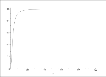
Figure 1: The quotient $[(\Delta J_{1,2})^{2}_{\textrm{phy}}-(\Delta J_{1,2})^{2}_{\textrm{kin}}]/(\Delta J_{1,2})^{2}_{\textrm{kin}}$, plotted as a function of $x=|\alpha_{2}|$. The constant that fixes the energy difference is set to $k=10$. Note that the ratio approaches 1/2, and is very close to 1/2 even when $|\alpha_{2}|$ is not very large.

It is straightforward to verify that the expectation values of $\hat{J}_{\pm}$ —and therefore of $\hat{J}_{1,2}$— in the physical coherent states coincide with the classical values:

$$\langle\hat{J}_{1,2}\rangle_{\textrm{phy}}=J_{1,2}|_{\textrm{cl}}\;.$$ (85)

For fluctuations we obtain

$$(\Delta\hat{J}_{1,2})^{2}_{\textrm{phy}}=\frac{|\alpha_{1}||\alpha_{2}|}{4}\left[\frac{\textrm{I}_{k-1}(2|\alpha_{1}||\alpha_{2}|)+\textrm{I}_{k+1}(2|\alpha_{1}||\alpha_{2}|)}{\textrm{I}_{k}(2|\alpha_{1}||\alpha_{2}|)}\right]+\frac{1}{2}$$ (86)

and

$$(\Delta\hat{J}_{1,2})^{2}_{\textrm{kin}}=\textstyle{\frac{1}{4}}\,(|\alpha_{1}|^{2}+|\alpha_{2}|^{2}+2)\;.$$ (87)

Therefore,

$$(\Delta\hat{J}_{1,2})^{2}_{\textrm{phy}}-(\Delta\hat{J}_{1,2})^{2}_{\textrm{kin}}=\frac{|\alpha_{1}||\alpha_{2}|}{4}\,\left[\frac{\textrm{I}_{k-1}(2|\alpha_{1}||\alpha_{2}|)+\textrm{I}_{k+1}(2|\alpha_{1}||\alpha_{2}|)}{\textrm{I}_{k}(2|\alpha_{1}||\alpha_{2}|)}\right]-\frac{1}{4}\,(|\alpha_{1}|^{2}+|\alpha_{2}|^{2})\;.$$ (88)

In Fig. 1, the fluctuations of $\hat{J}_{1,2}$ in the kinematical and physical states are compared. In particular, the quotient

$$\frac{(\Delta J_{1,2})^{2}_{\textrm{phy}}-(\Delta J_{1,2})^{2}_{\textrm{kin}}}{(\Delta J_{1,2})^{2}_{\textrm{kin}}}$$

is plotted as a function of $|\alpha_{2}|$ for $k=10$; the qualitative behavior is the same for other values of $k$. From the numerical investigations it is clear that the quotient approaches $1/2$ very fast as $|\alpha_{2}|$ grows. This means that the fluctuations in both types of coherent states are of the same order. However, in this example, the fluctuations are smaller in the kinematical coherent states than in the physical states and the difference remains bounded away from zero. However, it is clear that if the initial kinematical coherent states are chosen with tolerances $2\delta_{i}/3$, $\epsilon_{i}$, we would be guaranteed that the group averaged physical states will be semi-classical with desired tolerances $\delta_{i}$ and $\epsilon_{i}$.

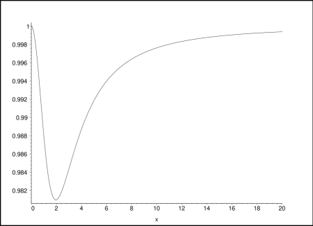
Figure 2: The quotient $\langle\hat{J}_{3}\rangle_{\textrm{phy}}/(J_{3})_{\textrm{cl}}$, plotted as a function of $x=|\alpha_{2}|$. The constant that fixes the energy difference is set to $k=10$. Notice that the ratio is very close to one even for values of $|\alpha_{2}|$ that are not that large.

Finally, for completeness, let us consider the quantum observable $\hat{J}_{3}=\frac{1}{2}\,(\hat{a}_{1}^{\dagger}\,\hat{a}_{1}+\hat{a}_{2}^{\dagger}\,\hat{a}_{2})$. For the expectation value, we have:

$$\langle\hat{J}_{3}\rangle_{\textrm{phy}}=\frac{1}{2}\left[\,|\alpha_{1}|^{2}\left|\frac{\alpha_{2}}{\alpha_{1}}\right|\,\frac{\textrm{I}_{k-1}(2|\alpha_{1}||\alpha_{2}|)}{|\alpha_{1}/\alpha_{2}|^{k}\,\textrm{I}_{k}(2|\alpha_{1}||\alpha_{2}|)}+|\alpha_{2}|^{2}\left|\frac{\alpha_{1}}{\alpha_{2}}\right|\,\frac{\textrm{I}_{k+1}(2|\alpha_{1}||\alpha_{2}|)}{|\alpha_{1}/\alpha_{2}|^{k}\,\textrm{I}_{k}(2|\alpha_{1}||\alpha_{2}|)}\right].$$ (89)

Since $|\alpha_{1}|^{2}=k+|\alpha_{2}|^{2}$, one can evaluate the last expression as a function of $k$ and $|\alpha_{2}|$ and compare it with the classical value. The quotient $(\langle\hat{J}_{3}\rangle_{\textrm{phy}})/(J_{3}|_{\textrm{cl}})$ is plotted in Fig. 2. As can be seen, already for small values of $k$ and $|\alpha_{2}|$, this quantity is very close to one; physical coherent states approximate very well the classical values of the Dirac observables we have chosen.

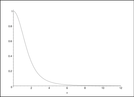
Figure 3: The quotient $[(\Delta\hat{J}_{3})^{2}_{\textrm{kin}}-(\Delta\hat{J}_{3})^{2}_{\textrm{phy}}]/(\Delta\hat{J}_{3})^{2}_{\textrm{kin}}$, plotted as a function of $x=|\alpha_{2}|$. The constant that fixes the energy difference is set to $k=10$. Note that the physical fluctuations are smaller and very rapidly approach the kinematical ones.

The fluctuation of $\hat{J}_{3}$ can be obtained by considering the expectation value

$$\langle\hat{J}^{2}_{3}\rangle_{\textrm{phy}}=\frac{1}{4}\left[|\alpha_{1}||\alpha_{2}|\left(\frac{\textrm{I}_{k-1}+\textrm{I}_{k+1}}{\textrm{I}_{k}}\right)+|\alpha_{1}|^{2}|\alpha_{2}|^{2}\left(\frac{\textrm{I}_{k-2}+2\textrm{I}_{k}+\textrm{I}_{k+2}}{\textrm{I}_{k}}\right)\right].$$ (90)

With this expression we can again analyze the behavior of $(\Delta\hat{J}_{3})^{2}_{\textrm{phy}}$ and compare it with the kinematical fluctuation. This comparison is shown in Fig. 3, where the quotient

$$\frac{(\Delta\hat{J}_{3})^{2}_{\textrm{kin}}-(\Delta\hat{J}_{3})^{2}_{\textrm{phy}}}{(\Delta\hat{J}_{3})^{2}_{\textrm{kin}}}$$

is plotted. Again the two fluctuations are of the same order. The main difference with the fluctuations of $\hat{J}_{1}$, $\hat{J}_{2}$ is that now the fluctuations in the physical states are smaller but they very rapidly approach those in the kinematical coherent states. Therefore the physical states are guaranteed to be semi-classical with respect to $\hat{J}_{3}$. Thus, although the detailed behavior of $\hat{J}_{3}$ is rather different from the one of $\hat{J}_{1}$ and $\hat{J}_{2}$, the physical states are again semi-classical also with respect to $\hat{J}_{3}$.

To summarize, by restricting the initial kinematical coherent states to have suitably small tolerances, the group averaged physical states can be guaranteed to be semi-classical for any specified choice of tolerances.

VI Discussion and Outlook

Let us begin with a brief summary of results. In section III we clarified two issues concerning the notion of semi-classical states. The clarifications in turn led us to a criterion under which states $\Psi^{\textrm{phy}}_{\alpha}$ obtained by group averaging suitable kinematical coherent states $\Psi_{\alpha}$ can be regarded as semi-classical in ${\cal H}_{\textrm{phy}}$. In sections IV and V we saw that the criterion is satisfied if the constraint sub-manifold $\bar{\Gamma}$ is the level surface of a linear function on $\Gamma$ or a quadratic function satisfying certain conditions. Thus, the group averaging procedure offers a concrete and potentially powerful strategy to construct physical semi-classical states for a class of constrained systems.

In the examples with quadratic constraints the result could not have been foreseen on general grounds. Indeed, even in retrospect we do not have a general understanding of ‘why’ the strategy works. It is particularly surprising that, in certain cases, the group averaging procedure even reduces the fluctuations of Dirac observables. Now, all examples we considered have the feature that $\hat{U}(\lambda)\Psi_{\alpha}$ is again a coherent state, peaked at a point $\alpha(\lambda)$ of the phase space ${\Gamma}$ on the orbit of the gauge transformation generated by the classical constraint $C$. This will not hold generally. Is this feature perhaps the key to the ‘nicer than expected’ behavior of the group averaged coherent states? For example, since the value of any classical Dirac observable ${\cal O}$ is constant along a gauge orbit, this feature implies that the expectation values $\langle\hat{U}(\lambda)\Psi_{\alpha}\,|\,\hat{\cal O}\,|\,\hat{U}(\lambda)\Psi_{\alpha}\rangle$ are all equal to the values ${\cal O}(\alpha)$ of ${\cal O}$ at the classical point $\alpha\in{\Gamma}$. Note, however, that it is not these expectation values that dictate the calculation of $\langle\Psi_{\alpha}^{\textrm{phy}}\,|\,\hat{\cal O}\,|\,\Psi_{\alpha}^{\textrm{phy}}\rangle$. As we saw in section V, the calculation is governed, rather, by a delicate interplay between the cross matrix elements $\langle\Psi_{\alpha}\,|\,\hat{\cal O}\,|\,\hat{U}(\lambda)\Psi_{\alpha}\rangle$ and the norm of the physical state $\Psi^{\textrm{phy}}_{\alpha}$. Neither of these by itself has any simple relation to the value ${\cal O}(\alpha)$ of the classical Dirac observable. Thus, while the specific property now under consideration of our class of constraints did simplify the detailed calculations, it does not seem to suffice to ensure semi-classicality of $\Psi^{\textrm{phy}}_{\alpha}$. Indeed, there are examples of quadratic constraints —such as those in the Bianchi I model— which do not share this property but where the group averaging procedure is again useful in constructing physical semi-classical states bbc . It would be extremely useful to understand the underlying mechanism which makes the group averaging strategy successful in a rather diverse class of examples and prove a general result which guarantees success for a wide class of constraints.

The following heuristics suggest that this may well be possible. In the case of a generic constraint, one can simply choose the constraint function itself as the first canonical coordinate, say $q_{1}$, on the linear phase space ${\Gamma}$, and then supplement it with other suitably chosen functions (tailored to one’s choice of Dirac observables) to form a canonical coordinate system $(q_{i},p_{i})$. Then, as in section IV, physical states would have a simple distributional form in the $q$-representation: $\Psi^{\textrm{phy}}(q)=\delta(q_{1})f(q_{2},...,q_{D})$. However, in the general case, this canonical chart would not be adapted to the linearity of the phase space, whence it would be difficult to identify coherent states in this representation. Nonetheless, it should be possible to introduce some notion of kinematical semi-classical states $\Psi^{\textrm{kin}}_{\alpha}(q)$. Then the group averaging procedure would lead to states $\Psi^{\textrm{phy}}_{\alpha}(q)=\delta(q_{1})\Psi^{\textrm{kin}}_{\alpha}(q_{2},...,q_{D})$. These are natural candidates for physical semi-classical states. For, Dirac observables would act only on the variables $q_{2},\ldots,q_{D}$, whence there could be a simple relation between their expectation values in $\Psi^{\textrm{kin}}_{\alpha}(q)$ and $\Psi^{\textrm{phy}}_{\alpha}(q)$ needed to establish their semi-classicality. A number of non-trivial technical problems need to be overcome to determine whether these heuristic ideas can be made precise. Nonetheless, they indicate that there may well be a much more general underlying structure responsible for the success of the group averaging method in the few examples discussed in this paper.

References

- (1) J. R. Klauder, “Coherent State Quantization of Constraint Systems”, Ann. Phys. 254, 419-453 (1997), and arXiv:quant-ph/9604033.
- (2) A. Kempf and J. R. Klauder, “On the implementation of constraints through projection operators”, J. Phys. A 34, 1019 (2001), and arXiv:quant-ph/0009072.
- (3) J. R. Klauder, “Universal procedure for enforcing quantum constraints”, Nucl. Phys. B547, 397 (1999) and arXiv:hep-th/9901010.
- (4) J. R. Klauder, “Phase space geometry in classical and quantum mechanics”, arXiv:quant-ph/0112010.
- (5) M. C. Ashworth, “Coherent state approach to time-reparametrization invariant systems”, Phys. Rev. A 57, 2357 (1998), and arXiv:quant-ph/9611026.
- (6) D. Marolf, “Group averaging and refined algebraic quantization: Where are we now?”, arXiv:gr-qc/0011112; D. Giulini and D. Marolf, “On the generality of refined algebraic quantization”, Class. Quantum Grav. 16, 2479 (1999), and arXiv:gr-qc/9812024.
- (7) C. Rovelli, “Quantum mechanics without time: A model”, Phys. Rev. D 42, 2638 (1990).
- (8) A. Ashtekar and R.S. Tate, “An algebraic extension of Dirac quantization: Examples”, J. Math. Phys. 35, 6434 (1994), and arXiv:gr-qc/9405073.
- (9) K. Kuchař, “Canonical quantization of cylindrical gravitational waves”, Phys. Rev. D 4, 955 (1971).
- (10) A. Ashtekar and M. Pierri, “Probing quantum gravity through exactly soluble midi-superspaces. I”, J. Math. Phys. 37, 6250 (1996), and arXiv:gr-qc/9606085.
- (11) A. Ashtekar, “Large quantum gravity effects: Unforeseen limitations of the classical theory”, Phys. Rev. Lett. 77, 4864 (1996), and arXiv:gr-qc/9610008.
- (12) R. Gambini and J. Pullin, “Large quantum gravity effects: Backreaction on matter”, Mod. Phys. Lett. A12, 2407 (1997), and arXiv:gr-qc/9703088.
- (13) See, e.g., J.M. Isidro, “Coherent states and duality”, Phys. Lett. A301 210 (2002), and arXiv:quant-ph/0204128.
- (14) B. Bolen, L. Bombelli and A. Corichi, “Semiclassical states in quantum cosmology: Bianchi I coherent states”, Class. Quantum Grav. 21, 4087 (2004), and arXiv:gr-qc/04040004.