The one-loop effective action in $\phi^{4}$ theory coupled non-linearly with curvature power and dynamical origin of cosmological constant

Abstract

The functional formulation and one-loop effective action for scalar self-interacting theory non-linearly coupled with some power of the curvature are studied. After the explicit one-loop renormalization at weak curvature, we investigated numerically the phase structure for such unusual $\phi^{4}$ theory. It is demonstrated the possibility of curvature-induced phase transitions for positive values of the curvature power, while for negative values the radiative symmetry breaking does not take place. The dynamical mechanism for the explanation of the current smallness of the cosmological constant is presented for several models from the class of theories under consideration.

1 Introduction

The current stage of theoretical cosmology and, in particularly, the dark energy problem calls to consideration of new field theory models which maybe useful for the explanation of the universe acceleration. In the situation when the attempts to use the well-known classes of field theories as candidates for dark energy (dark matter) are not quite successful, such strategy seems to be justified. Moreover, one should bear in mind that number of problems of the early time cosmology (say, the fundamental cosmological constant problem) are still too far from the resolution. The (old or new) field theoretical model which should include also gravitation itself should solve these problems at once (at least, in the regime where one can still neglect the quantum gravity effects).

In the recent paper [1] the class of dark energy models where dark energy (scalar or spinor field theory, etc) couples with some power of the curvature has been proposed. It has been demonstrated on the example of scalar Lagrangian coupled with the power of curvature that such modification of gravity-matter coupling term may explain not only the current cosmic speed-up, but also the dark energy dominance assisted by gravity. On the same time, theories of similar nature have been recently proposed as good candidate for dynamical resolution of the cosmological constant problem [2, 3] (see also [4]). Of course, such models are not standard ones, in the sense that they are not multiplicatively renormalizable in curved spacetime [5]. Hence, they should be considered as kind of effective theories (without clear understanding of their origin and their relation with more fundamental string/M-theory).

In the present paper we continue the study of the properties of such models on the example of scalar self-interacting theory non-linearly coupled with some power of the curvature. Admitting the discrete symmetry which prohibits odd powers of scalar in the potential, the effective action formulation (section 2) is developed in close analogy with multiplicatively renormalizable theories [5]. Using Riemann normal coordinate expansion, the modified Green function is evaluated at weak curvature limit (section 3). (We work in linear curvature approximation what is expected to be appropriate for the study of quantum effects in the inflationary universe and in late-time, dark energy universe). Subsequently, this Green function is used for the calculation of the one-loop effective action in the same limit (section 4). After the one-loop renormalization of the effective action done in section 5, one arrives at finite expression which is used for the numerical study of the phase structure in FRW universe. The number of examples explicitly demonstrates the behaviour of the effective potential for such effective theory. In particularly, it is shown the possibility of curvature-induced phase transitions in the model under discussion (section 6). It is indicated that radiative corrections are not very relevant at weak curvature.

Finally, in section 7 it is shown that scalar theory under consideration may serve also for dynamical resolution of cosmological constant problem. The explicit choice of parameters (which maybe considered as kind of fine-tuning) giving such dynamical resolution is presented. It is interesting that radiative corrections are not relative for such a mechanism. Some discussion and outlook are given in the last section.

2 $\phi^{4}$ theory coupled non-linearly with curvature power

We extend the $\phi^{4}$ theory which is the simplest model where the spontaneous symmetry breaking takes place. One of the possible couplings of scalar Lagrangian with curvature (at some power) maybe included into the starting action:

$$S=\int d^{D}x\ \sqrt{-g}\left[\frac{1}{2\kappa^{2}}R+\left(\frac{R}{M^{2}}\right)^{\alpha}{\cal L}_{d}\right].$$ (1)

where $M$ is an arbitrary mass scale, $g$ is the determinant of the metric tensor $g_{\mu\nu}$ and ${\cal L}_{d}$ is the ordinary Lagrangian density of the $\phi^{4}$ theory,

$${\cal L}_{d}(\phi_{0})=\frac{1}{2}\phi_{0;\mu}{\phi_{0}}^{;\mu}-\frac{\xi_{0}R}{2}\phi_{0}^{2}+\frac{\mu_{0}^{2}}{2}\phi_{0}^{2}-\frac{\lambda_{0}}{4!}\phi_{0}^{4},$$ (2)

where $\phi_{0}$ is a real scalar field. Our sign convention for the metric is $(+---\cdots)$ and follows the notation of Birrell and Davies [6]. If the spacetime curvature is constant, the non-linear curvature coupling disappears by the transformation

$$\phi \rightarrow \left(\frac{R}{M^{2}}\right)^{-\alpha/2}\phi,$$ (3)

$$\lambda_{0} \rightarrow \left(\frac{R}{M^{2}}\right)^{\alpha}\lambda_{0}.$$ (4)

We are interested in a non-trivial effect of the non-linear curvature coupling. It will be found in a non-static and/or inhomogeneous spacetime. Note that the non-linear coupling of above sort has been proposed in Ref. [1] (see also related model in [7]) as the model of dark energy which naturally resolves the problem of dark energy dominance in the current universe.

The Lagrangian is invariant under the discrete transformation,

$$\phi\rightarrow-\phi.$$ (5)

This symmetry prevents the Lagrangian from having $\phi^{3}$ terms. A non-vanishing expectation value for the field $\phi$ breaks the discrete symmetry spontaneously. To evaluate the expectation value for $\phi$ we calculate the effective action.

We start from the generating functional $W[J]$. The generating functional of the theory is given by

$$e^{\frac{i}{\hbar}W[J]}\equiv\int{\cal D}\phi_{0}\ e^{\frac{i}{\hbar}S+\frac{i}{\hbar}\int d^{D}x\sqrt{-g}\phi_{0}J}$$ (6)

In the presence of the source $J$ the classical equation of motion becomes

$$\left.\frac{\delta S}{\delta\phi_{0}(x)}\right|_{\phi_{0}=\phi_{b}}=-J(x).$$ (7)

In curved spacetime the functional derivative is defined by

$$S[\phi_{0}+\delta\phi]-S[\phi_{0}]=\int d^{D}x\sqrt{-g}\frac{\delta S}{\delta\phi_{0}(x)}\delta\phi_{0}(x).$$ (8)

We divide the field $\phi_{0}$ into a classical background $\phi_{b}$ which satisfies the Eq.(7) and a quantum fluctuation $\tilde{\phi}$,

$$\phi_{0}=\phi_{b}+\hbar^{1/2}\tilde{\phi}.$$ (9)

In terms of $\phi_{b}$ and $\tilde{\phi}$ the action $S[\phi_{0}]$ is rewritten as

$$S[\phi_{0}] = S[\phi_{b}+\hbar^{1/2}\tilde{\phi}]$$ (10)

$$= S[\phi_{b}]+\int d^{D}x\sqrt{-g}\left.\frac{\delta S[\phi_{0}]}{\delta\phi_{0}(x)}\right|_{\phi_{0}=\phi_{b}}\hbar^{1/2}\tilde{\phi(x)}$$

$$+\frac{\hbar}{2}\int d^{D}x\int d^{D}y\sqrt{-g(x)}\sqrt{-g(y)}\tilde{\phi}(x)iG_{d}^{-1}(x,y)\tilde{\phi}(y)+\mbox{O}({\tilde{\phi}^{3}})$$

$$= S[\phi_{b}]-\int d^{D}x\sqrt{-g}J(x)\hbar^{1/2}\tilde{\phi}(x)$$

$$+\frac{\hbar}{2}\int d^{D}x\int d^{D}y\sqrt{-g(x)}\sqrt{-g(y)}\tilde{\phi}(x)iG_{d}^{-1}(x,y)\tilde{\phi}(y)$$

$$+\mbox{O}({\hbar^{3/2}\tilde{\phi}^{3}}),$$

where $G_{d}^{-1}(x,y)$ is given by

$$iG_{d}^{-1}(x,y) \equiv \frac{\delta^{2}S[\phi_{0}]}{\delta\phi_{0}(x)\delta\phi_{0}(y)}$$ (11)

$$= -\sqrt{-g(x)}\left[\left(\frac{R}{M^{2}}\right)^{\alpha}\left(\square+\xi_{0}R-\mu_{0}^{2}+\frac{\lambda_{0}}{2}\phi_{b}^{2}\right)\right.$$

$$+\left.\alpha\left(\frac{R}{M^{2}}\right)^{\alpha-1}\frac{R_{;\mu}}{M^{2}}\nabla^{\mu}\right].$$

Therefore the generating functional (6) is expanded to be

$$e^{\frac{i}{\hbar}W[J]} = e^{\frac{i}{\hbar}\left(S[\phi_{b}]-\int d^{D}x\sqrt{-g}J(x)\phi_{b}(x)\right)}$$ (12)

$$\times\int{\cal D}\tilde{\phi}\ e^{\frac{i}{2}\int d^{D}x\int d^{D}y\sqrt{-g(x)}\sqrt{-g(y)}\tilde{\phi}(x)iG_{d}^{-1}(x,y)\tilde{\phi}(y)+\mbox{O}(\hbar^{1/2})}$$

Performing the path-integral,

$$\int{\cal D}\tilde{\phi}\ e^{\frac{i}{2}\int d^{D}x\int d^{D}y\sqrt{-g(x)}\sqrt{-g(y)}\tilde{\phi}(x)iG_{d}^{-1}(x,y)\tilde{\phi}(y)}=\left[\mbox{Det}\ iG_{d}^{-1}\right]^{-1/2},$$ (13)

we obtain the generating functional

$$W[J]=S[\phi_{b}]-\int d^{D}x\sqrt{-g}J(x)\phi_{b}(x)-\frac{i\hbar}{2}\ln\left[\mbox{Det}\ iG_{d}^{-1}\right]+\mbox{O}(\hbar^{3/2}).$$ (14)

The effective action $\Gamma[\phi_{c}]$ is given by the Legendre transform of $W[J]$,

$$\Gamma[\phi_{c}]\equiv W[J]-\int d^{D}x\sqrt{-g}\phi_{c}(x)J(x),$$ (15)

where $\phi_{c}$ denotes the expectation value of $\phi_{0}$ in the presence of the source $J$,

$$\phi_{c}\equiv\frac{\delta W[J]}{\delta J}.$$ (16)

Substituting Eq. (14) to Eq. (15) we find that the effective action is expanded to be

$$\Gamma[\phi_{c}]=S[\phi_{c}]-\frac{i\hbar}{2}\ln\left[\mbox{Det}\ iG_{d}^{-1}\right]+\mbox{O}(\hbar^{3/2}).$$ (17)

In the path integral formalism the expectation value of $\phi_{0}$ in the ground state satisfies

$$\langle\phi_{0}\rangle\equiv\lim_{J\rightarrow 0}\frac{\delta W[J]}{\delta J}.$$ (18)

This equation is rewritten as

$$\left.\frac{\delta\Gamma[\phi_{c}]}{\delta\phi_{c}}\right|_{\phi_{c}\rightarrow\langle\phi_{0}\rangle}=0,$$ (19)

where we have used the relation

$$\frac{\delta\Gamma[\phi_{c}]}{\delta\phi_{c}}=J.$$ (20)

The equation (19) is called the gap equation. The solution of the gap equation shows the presence of stationary points of the effective action $\Gamma[\phi_{c}]$. Thus, the phase structure of the theory maybe found by observing the stationary points of $\Gamma[\phi_{c}]$ (for a review of the quantum field theory in curved spacetime, see Ref. [5]).

3 Scalar Green function at the weak curvature limit

Following the procedure developed in Refs. [8, 9], we solve the Klein-Gordon equation and calculate the Green function $G_{d}$ (11) at the weak curvature limit. Note that in Green function calculation we actually work in the expansion on the curvatures what is known to be appropriate for the study of quantum effects in the inflationary universe and also in late-time, dark energy universe.

The Green function $G_{d}$ satisfies the modified Klein-Gordon equation,

$$\sqrt{-g(x)}\left[\left(\frac{R}{M^{2}}\right)^{\alpha}\left(\square+\xi_{0}R-\mu_{0}^{2}+\frac{\lambda_{0}}{2}\phi^{2}\right)\right.$$

$$\hskip 56.9055pt+\left.\alpha\left(\frac{R}{M^{2}}\right)^{\alpha-1}\frac{R_{;\mu}}{M^{2}}\nabla^{\mu}\right]iG_{d}(x,x^{\prime})=\delta^{D}(x-x^{\prime}).$$ (21)

For a practical calculations it is more convenient to introduce $G(x,x^{\prime})$ and $H_{x}$ which are defined by

$$G(x,x^{\prime})\equiv(-g)^{1/4}(x)\left(\frac{R(x)}{M^{2}}\right)^{\alpha/2}iG_{d}(x,x^{\prime})(-g)^{1/4}(x^{\prime})\left(\frac{R(x^{\prime})}{M^{2}}\right)^{\alpha/2},$$ (22)

and

$$H_{x} = (-g)^{1/4}(x)\left(\frac{R(x)}{M^{2}}\right)^{\alpha/2}\sqrt{-g(x)}\left[\left(\square+\xi_{0}R-\mu_{0}^{2}+\frac{\lambda_{0}}{2}\phi^{2}\right)\right.$$ (23)

$$\hskip 51.21495pt+\left.\alpha\left(\frac{R}{M^{2}}\right)^{-1}\frac{R_{;\mu}}{M^{2}}\nabla^{\mu}\right](-g)^{-1/4}(x)\left(\frac{R(x)}{M^{2}}\right)^{-\alpha/2},$$

In terms of $G(x,x^{\prime})$ and $H_{x}$ the Klein-Gordon equation (21) reads

$$H_{x}G(x,x^{\prime})=\delta^{D}(x-x^{\prime}).$$ (24)

After some calculations the Hamiltonian density $H_{x}$ is rewritten as

$$H_{x}=\partial_{\mu}g^{\mu\nu}\partial_{\nu}+\alpha\frac{R_{;\mu}}{R}\partial^{\mu}+V_{x},$$ (25)

where the potential $V_{x}$ is given by

$$V_{x} = \left[(-g)^{1/4}\partial_{\mu}(-g)^{1/2}g^{\mu\nu}\partial_{\nu}(-g)^{-1/4}\right]+\xi_{0}R-\mu_{0}^{2}+\frac{\lambda_{0}}{2}\phi^{2}$$ (26)

$$+\alpha\frac{R_{;\mu}}{R}\left[(-g)^{-1/4}\partial^{\mu}(-g)^{1/4}\right]-\frac{\alpha}{2}\left(\frac{\alpha}{2}-1\right)\frac{R^{;\mu}R_{;\mu}}{R^{2}}-\frac{\alpha}{2}\frac{\square R}{R}.$$

Here we adopt the Riemann normal coordinate expansion [10]. We set the origin of the coordinates at $x$ and write $y=x-x^{\prime}$ and neglect terms proportional to $y^{a}$, $a\geq 2$. Hence, the Eq.(24) is rewritten as

$$\left(\eta_{\mu\nu}\partial^{\mu}\partial^{\nu}+\zeta_{\mu}\partial^{\mu}+\xi_{\mu\nu}y^{\mu}\partial^{\nu}+\chi^{2}+\beta_{\mu}y^{\mu}\right)G(y)=\delta^{D}(y),$$ (27)

where

$$\zeta_{\mu} = \left.\alpha\frac{R_{;\mu}}{R}\right|_{y=0},$$ (28)

$$\xi_{\mu\nu} = \left.\alpha\left(\frac{R_{;\mu\nu}}{R}-\frac{R_{;\mu}R_{;\nu}}{R^{2}}\right)\right|_{y=0},$$ (29)

$$\chi^{2} = \left.\left[-\mu_{0}^{2}+\frac{\lambda_{0}}{2}\phi^{2}+\left(\xi_{0}-\frac{1}{6}\right)R-\frac{\alpha}{2}\left(\frac{\alpha}{2}-1\right)\frac{R^{;\mu}R_{;\mu}}{R^{2}}-\frac{\alpha}{2}\frac{\square R}{R}\right]\right|_{y=0}$$ (30)

$$\equiv -\mu_{0}^{2}+U,$$

$$\beta_{\mu} = \left.\left(U_{;\mu}+\frac{\alpha}{6}\frac{R^{;\nu}}{R}R_{\mu\nu}\right)\right|_{y=0}.$$ (31)

Performing the Fourier transformation

$$G(y)=\int\frac{d^{D}p}{(2\pi)^{D}}e^{ipy}\tilde{G}(p),$$ (32)

one finds that the equation (27) becomes

$$\left(-p^{2}+i\zeta_{\mu}p^{\mu}+\xi_{\mu\nu}p^{\nu}\partial_{p}^{\mu}+\chi^{2}-i\beta_{\mu}\partial_{p}^{\mu}\right)\tilde{G}(p)=1.$$ (33)

First we consider the solution for a positive $\chi^{2}$. In this case the following proper-time form for the solution of Eq.(33) is assumed

$$\tilde{G}(p)=\int^{\infty}_{0}dse^{-\chi^{2}s}e^{p^{\mu}A_{\mu\nu}(s)p^{\nu}+iB_{\mu}(s)p^{\mu}+C(s)}.$$ (34)

Substituting this into the Eq.(33) one obtains

$$\int^{\infty}_{0}ds\left(-p^{2}+i\zeta_{\mu}p^{\mu}+\xi_{\mu\nu}X^{\mu}p^{\nu}+\chi^{2}-i\beta_{\mu}X^{\mu}\right)$$

$$\hskip 28.45274pt\times e^{-\chi^{2}s}e^{p^{\mu}A_{\mu\nu}(s)p^{\nu}+iB_{\mu}(s)p^{\mu}+C(s)}$$

$$=1,$$ (35)

where

$$X^{\mu}=A^{\mu\nu}p_{\nu}+p_{\nu}A^{\mu\nu}+iB^{\mu}.$$ (36)

On the other hand, there is an identity

$$-\int^{\infty}_{0}ds\frac{d}{ds}e^{-\chi^{2}s}e^{p^{\mu}A_{\mu\nu}(s)p^{\nu}+iB_{\mu}(s)p^{\mu}+C(s)}$$

$$=\int^{\infty}_{0}ds\left(\chi^{2}-p^{\mu}\frac{dA_{\mu\nu}}{ds}p^{\nu}-i\frac{dB_{\mu}}{ds}p^{\mu}-\frac{dC}{ds}\right)$$

$$\hskip 28.45274pt\times e^{-\chi^{2}s}e^{p^{\mu}A_{\mu\nu}(s)p^{\nu}+iB_{\mu}(s)p^{\mu}+C(s)}$$

$$=1,$$ (37)

Comparing the Eq.(35) with the Eq.(37), the simultaneous differential equations are obtained

$$\frac{dA_{\mu\nu}}{ds} = 1-\xi_{\mu\rho}({A^{\rho}}_{\nu}+{A_{\nu}}^{\rho}),$$ (38)

$$\frac{dB_{\mu}}{ds} = -\zeta_{\mu}-\xi_{\mu\rho}B^{\rho}-\beta_{\rho}({A^{\rho}}_{\nu}+{A_{\nu}}^{\rho}),$$ (39)

$$\frac{dC}{ds} = -\beta_{\mu}B^{\mu}.$$ (40)

The solutions of these differential equations are found to be

$$A = \frac{1}{2}\xi^{-1}+C_{1}e^{-2\xi s},$$ (41)

$$B = -\xi^{-1}\zeta+\beta\xi^{-2}+C_{2}e^{-\xi s}-2\beta\xi^{-1}C_{1}e^{-2\xi s},$$ (42)

$$C = \beta\xi^{-1}\zeta s-(\beta\xi^{-1})^{2}s+\beta\xi^{-1}C_{2}e^{-\xi s}-(\beta\xi^{-1})^{2}C_{1}e^{-2\xi s}$$ (43)

$$+C_{3},$$

where $C_{1}$, $C_{2}$ and $C_{3}$ are constant matrix parameters which are determined by the boundary conditions. In the flat space time, $R\rightarrow 0$, Eq.(33) must reproduce a Klein-Gordon equation in the Minkowski space. Thus, the functions $A$, $B$ and $C$ must satisfy

$$A \rightarrow s,$$ (44)

$$B \rightarrow 0,$$ (45)

$$C \rightarrow 0,$$ (46)

at the limit $\zeta$, $\xi$, $\beta\rightarrow 0$.

These boundary conditions fix the parameters $C_{1}$, $C_{2}$ and $C_{3}$ to be

$$C_{1} = -\frac{1}{2}\xi^{-1},$$ (47)

$$C_{2} = -2\beta\xi^{-2}+\xi^{-1}\zeta,$$ (48)

$$C_{3} = \frac{3}{2}(\beta\xi^{-1})(\beta\xi^{-2})-\beta\xi^{-2}\zeta.$$ (49)

Therefore the functions $A$, $B$ and $C$ are simplified to

$$A = \frac{1}{2}\xi^{-1}(1-e^{-2\xi s}),$$ (50)

$$B = -\xi^{-1}\zeta(1-e^{-\xi s})+\beta\xi^{-2}(1-e^{-\xi s})^{2},$$ (51)

$$C = -\beta\xi^{-2}\zeta(1-e^{-\xi s}-\xi s)$$ (52)

$$+2(\beta\xi^{-1})(\beta\xi^{-2})\left[\left(1-e^{-\xi s}-\xi s\right)-\frac{1}{4}\left(1-e^{-2\xi s}-2\xi s\right)\right].$$

Since the parameters $\zeta$, $\xi$ and $\beta$ are small enough at the weak curvature limit, we neglect the higher order term about these parameters for a small $s$ and get

$$A \sim s-\xi s^{2},$$ (53)

$$B \sim -\zeta s+\beta s^{2},$$ (54)

$$C \sim \frac{1}{2}\beta\zeta s^{2}-\frac{1}{3}\beta^{2}s^{3}\sim 0.$$ (55)

Inserting these solutions into Eq.(34), the Green function $\tilde{G}(p)$ follows

$$\tilde{G}(p)=\int^{\Lambda}_{0}dse^{-(p^{\mu}\xi_{\mu\nu}p^{\nu}-i\beta_{\mu}p^{\mu})s^{2}+(p^{2}-\chi^{2}-i\zeta_{\mu}p^{\mu})s},$$ (56)

where a scale $\Lambda\sim\sqrt{|R|/M^{2}}$ is introduced. It corresponds to the upper limit where we can neglect the higher order term about the parameters $\zeta$, $\xi$ and $\beta$. Since the integrand becomes smaller and smaller above the scale $\Lambda$, we drop the contribution from the region above $\Lambda$. It is straightforward to extend above analysis to a negative $\chi^{2}$ and obtain

$$\tilde{G}(p)=\int^{-\Lambda}_{0}dse^{-(p^{\mu}\xi_{\mu\nu}p^{\nu}-i\beta_{\mu}p^{\mu})s^{2}+(p^{2}-\chi^{2}-i\zeta_{\mu}p^{\mu})s},$$ (57)

Integrating over $s$ in Eq.(56) and (57), it follows

$$\tilde{G}(p) = \sqrt{\frac{\pi}{4(p^{\mu}\xi_{\mu\nu}p^{\nu}-i\beta_{\mu}p^{\mu})}}\exp\left[\frac{(p^{2}-\chi^{2}-i\zeta_{\mu}p^{\mu})^{2}}{4(p^{\mu}\xi_{\mu\nu}p^{\nu}-i\beta_{\mu}p^{\mu})}\right]$$ (58)

$$\times\left[1+\mbox{erf}\left(-\mbox{\scriptsize sgn}(\chi^{2})\frac{p^{2}-\chi^{2}-i\zeta_{\mu}p^{\mu}}{\sqrt{4(p^{\mu}\xi_{\mu\nu}p^{\nu}-i\beta_{\mu}p^{\mu})}}\right)\right],$$

where erf$(z)$ is the error function. In the configuration space the Green function $G(y)$ reads

$$G(y)=\int^{\mbox{\scriptsize sgn}(\chi^{2})\Lambda}_{0}dse^{-\chi^{2}s}\int\frac{d^{D}p}{(2\pi)^{D}}e^{ip^{\mu}y_{\mu}}e^{p^{\mu}A_{\mu\nu}p^{\nu}+iB_{\mu}p^{\mu}}.$$ (59)

At the origin it reduces to

$$G(0) = \int^{\mbox{\scriptsize sgn}(\chi^{2})\Lambda}_{0}dse^{-\chi^{2}s}\int\frac{d^{D}p}{(2\pi)^{D}}e^{p^{\mu}A_{\mu\nu}p^{\nu}+iB_{\mu}p^{\mu}}$$ (60)

$$= \frac{i}{(2\pi)^{D}}\int^{\mbox{\scriptsize sgn}(\chi^{2})\Lambda}_{0}ds\left(\det\frac{A}{\pi}\right)^{-1/2}e^{-\frac{1}{4}BA^{-1}B-\chi^{2}s}.$$

To perform the momentum integral the Wick rotation maybe applied. Neglecting the higher order term about $\zeta$, $\xi$ and $\beta$, we obtain

$$G(0)\sim\frac{i}{(4\pi)^{D/2}}\int^{\mbox{\scriptsize sgn}(\chi^{2})\Lambda}_{0}\frac{ds}{s^{D/2}}\left(1+\frac{1}{2}\mbox{tr}\xi s\right)e^{-\chi^{2}s}.$$ (61)

Hence, the scalar Green function is found at small curvature. It will be used in the calculation of the one-loop effective action.

4 The one-loop effective action

The effective action of the present model is given by (17). Here we normalize the effective action to satisfy

$$\Gamma[\phi=0]=S[\phi=0].$$ (62)

In this normalization the one-loop effective action is given by

$$\Gamma[\phi]=S[\phi]-\frac{i\hbar}{2}\left[\ln\left\{\mbox{Det}\ iG_{d}^{-1}(\phi^{2})\right\}-\ln\left\{\mbox{Det}\ iG_{d}^{-1}(\phi^{2}=0)\right\}\right].$$ (63)

The right hand side of Eq. (63) contains a term proportional to

$$\ln\left\{\mbox{Det}\ iG_{d}^{-1}(\phi^{2})\right\}-\ln\left\{\mbox{Det}\ iG_{d}^{-1}(\phi^{2}=0)\right\}$$

$$=\mbox{Tr}\left\{\ln iG_{d}^{-1}(\phi^{2})\right\}-\mbox{Tr}\left\{\ln iG_{d}^{-1}(\phi^{2}=0)\right\}$$

$$=-\frac{\lambda_{0}}{2}\int d^{D}x(-g)\left(\frac{R}{M^{2}}\right)^{\alpha}\int^{\phi^{2}}_{0}dm^{2}\ iG_{d}(x,x;\phi^{2}=m^{2}).$$ (64)

From the Eq.(61) the Green function at the weak curvature limit is found to be

$$G(x,x;\phi^{2}=m^{2})=\frac{i}{(4\pi)^{D/2}}\int^{\mbox{\scriptsize sgn}(\chi^{2})\Lambda}_{0}\frac{ds}{s^{D/2}}\left(1+\frac{1}{2}\mbox{tr}\xi s\right)e^{-\chi^{2}(\phi^{2}=m^{2})s}.$$ (65)

The relationship between $G_{d}$ and $G$ is given by

$$iG_{d}(x,x;\phi^{2}=m^{2})=\frac{1}{\sqrt{-g(x)}}\left(\frac{R(x)}{M^{2}}\right)^{-\alpha}G(x,x;\phi^{2}=m^{2}).$$ (66)

The effective action at the weak curvature limit reduces to

$$\Gamma[\phi] = S[\phi]-\frac{\hbar\lambda_{0}}{4(4\pi)^{D/2}}$$

$$\times\int d^{D}x\sqrt{-g}\int^{\phi^{2}}_{0}dm^{2}\int^{\mbox{\scriptsize sgn}(\chi^{2})\Lambda}_{0}\frac{ds}{s^{D/2}}\left(1+\frac{1}{2}\mbox{tr}\xi s\right)e^{-\chi^{2}(\phi^{2}=m^{2})s}.$$

Integrating over $m^{2}$ one gets

$$\Gamma[\phi] = S[\phi]+\frac{\hbar}{2(4\pi)^{D/2}}\int d^{D}x\sqrt{-g}$$ (68)

$$\times\int^{\mbox{\scriptsize sgn}(\chi^{2})\Lambda}_{0}\frac{ds}{s^{D/2+1}}\left(1+\frac{1}{2}\mbox{tr}\xi s\right)\left(e^{-\chi^{2}(\phi^{2})s}-e^{-\chi^{2}(\phi^{2}=0)s}\right).$$

Performing the integration about $s$ and neglecting the higher order term about $1/\Lambda$, we get

$$\Gamma[\phi] = S[\phi]$$ (69)

$$+\frac{\hbar}{2(4\pi)^{D/2}}\Gamma\left(-\frac{D}{2}\right)\int d^{D}x\sqrt{-g}\left[(\chi^{2}(\phi^{2}))^{D/2}\left(1-\frac{D\mbox{tr}\xi}{4\chi^{2}(\phi^{2})}\right)\right.$$

$$\left.\hskip 56.9055pt-(\chi^{2}(\phi^{2}=0))^{D/2}\left(1-\frac{D\mbox{tr}\xi}{4\chi^{2}(\phi^{2}=0)}\right)\right].$$

The effective Lagrangian density is defined by

$$\Gamma[\phi]=\int d^{D}x\sqrt{-g}{\cal L}_{eff}.$$ (70)

From Eqs.(1) and (69) it is found to be

$${\cal L}_{eff} = \frac{1}{2\kappa^{2}}R+\left(\frac{R}{M^{2}}\right)^{\alpha}\left(\frac{1}{2}\phi_{0;\mu}{\phi_{0}}^{;\mu}-\frac{\xi_{0}R}{2}\phi_{0}^{2}+\frac{\mu_{0}^{2}}{2}\phi_{0}^{2}-\frac{\lambda_{0}}{4!}\phi_{0}^{4}\right)$$ (71)

$$+\frac{\hbar}{2(4\pi)^{D/2}}\Gamma\left(-\frac{D}{2}\right)\left[(\chi^{2}(\phi^{2}))^{D/2}\left(1-\frac{D\mbox{tr}\xi}{4\chi^{2}(\phi^{2})}\right)\right.$$

$$\left.-(\chi^{2}(\phi^{2}=0))^{D/2}\left(1-\frac{D\mbox{tr}\xi}{4\chi^{2}(\phi^{2}=0)}\right)\right].$$

with

$$\mbox{tr}\xi = \alpha\left(\frac{\square R}{R}-\frac{R^{;\mu}R_{;\mu}}{R^{2}}\right),$$ (72)

$$\chi^{2}(\phi^{2}) = -\mu_{0}^{2}+\frac{\lambda_{0}}{2}\phi^{2}+\left(\xi_{0}-\frac{1}{6}\right)R-\frac{\alpha}{2}\left(\frac{\alpha}{2}-1\right)\frac{R^{;\mu}R_{;\mu}}{R^{2}}-\frac{\alpha}{2}\frac{\square R}{R},$$ (73)

In the limit $\alpha\rightarrow 0$ and $R\rightarrow 0$ the effective Lagrangian density (71) reproduces the one in the Minkowski space.

5 The one-loop renormalization

The effective action (69) and the effective Lagrangian density (71) are divergent in two and four dimensions. To obtain the finite value we must renormalize the theory. (Remind that theory is not multiplicatively renormalizable in curved spacetime [5]). At the present order we impose the following renormalization conditions

$$\left.\frac{\partial^{2}\Gamma[\phi]}{\partial\phi^{2}}\right|_{\phi=M_{1}}\equiv\left(\frac{R}{M^{2}}\right)^{\alpha}(\mu_{r}^{2}-\xi_{r}R),$$ (74)

$$\left.\frac{\partial^{4}\Gamma[\phi]}{\partial\phi^{4}}\right|_{\phi=M_{2}}\equiv-\left(\frac{R}{M^{2}}\right)^{\alpha}\lambda_{r}.$$ (75)

where $M_{1}$ and $M_{2}$ are the renormalization scales. From these conditions one obtains the relationship between the renormalized parameters $\mu_{r}$, $\xi_{r}$, $\lambda_{r}$ and the bare ones $\mu_{0}$, $\xi_{0}$, $\lambda_{0}$.

$$\mu_{r}^{2}-\xi_{r}R = \mu_{0}^{2}-\xi_{0}R-\frac{\lambda_{0}}{2}M_{1}^{2}-\frac{\hbar}{2(4\pi)^{D/2}}\left(\frac{R}{M^{2}}\right)^{-\alpha}\lambda_{0}$$ (76)

$$\times\left\{\Gamma\left(1-\frac{D}{2}\right)(\chi^{2}(M_{1}^{2}))^{D/2-1}\right.$$

$$\left.\hskip 51.21495pt\times\left[1+\lambda_{0}M_{1}^{2}\left(\frac{D}{2}-1\right)(\chi^{2}(M_{1}^{2}))^{-1}\right]\right.$$

$$\left.+\frac{1}{2}\Gamma\left(2-\frac{D}{2}\right)(\chi^{2}(M_{1}^{2}))^{D/2-2}\right.$$

$$\left.\hskip 51.21495pt\times\left[1+\lambda_{0}M_{1}^{2}\left(\frac{D}{2}-2\right)(\chi^{2}(M_{1}^{2}))^{-1}\right]\mbox{tr}\xi\right\}$$

$$\equiv \mu_{0}^{2}-\xi_{0}R-\frac{\lambda_{0}}{2}M_{1}^{2}+\frac{\hbar}{2(4\pi)^{D/2}}\left(\frac{R}{M^{2}}\right)^{-\alpha}\lambda_{0}f(D,M_{1}),$$

$$\lambda_{r} = \lambda_{0}-\frac{\hbar}{2(4\pi)^{D/2}}\left(\frac{R}{M^{2}}\right)^{-\alpha}\lambda_{0}^{2}$$ (77)

$$\times\left\{\Gamma\left(2-\frac{D}{2}\right)(\chi^{2}(M_{2}^{2}))^{D/2-2}\left[3+6\lambda_{0}M_{2}^{2}\left(\frac{D}{2}-2\right)(\chi^{2}(M_{2}^{2}))^{-1}\right.\right.$$

$$\left.\left.\hskip 79.66771pt+\lambda_{0}^{2}M_{2}^{4}\left(\frac{D}{2}-2\right)\left(\frac{D}{2}-3\right)(\chi^{2}(M_{2}^{2}))^{-2}\right]\right.$$

$$\left.+\frac{1}{2}\Gamma\left(3-\frac{D}{2}\right)(\chi^{2}(M_{2}^{2}))^{D/2-3}\left[3+6\lambda_{0}M_{2}^{2}\left(\frac{D}{2}-3\right)(\chi^{2}(M_{2}^{2}))^{-1}\right.\right.$$

$$\left.\left.\hskip 79.66771pt+\lambda_{0}^{2}M_{2}^{4}\left(\frac{D}{2}-3\right)\left(\frac{D}{2}-4\right)(\chi^{2}(M_{2}^{2}))^{-2}\right]\mbox{tr}\xi\right\}$$

$$\equiv \lambda_{0}+\frac{\hbar}{2(4\pi)^{D/2}}\left(\frac{R}{M^{2}}\right)^{-\alpha}\lambda_{0}^{2}g(D,M_{2}).$$

By using these renormalized parameters the effective Lagrangian density (71) is rewritten as

$${\cal L}_{eff} = \frac{1}{2\kappa^{2}}R+\left(\frac{R}{M^{2}}\right)^{\alpha}\left(\frac{1}{2}\phi_{;\mu}{\phi}^{;\mu}-\frac{\xi_{r}R}{2}\phi^{2}+\frac{\mu_{r}^{2}}{2}\phi^{2}+\frac{\lambda_{r}}{4}M_{1}^{2}\phi^{2}-\frac{\lambda_{r}}{4!}\phi^{4}\right)$$ (78)

$$-\frac{\hbar}{4(4\pi)^{D/2}}\lambda_{r}f(D,M_{1})\phi^{2}+\frac{\hbar}{48(4\pi)^{D/2}}\lambda_{r}^{2}g(D,M_{2})(\phi^{4}-6M_{1}^{2}\phi^{2})$$

$$+\frac{\hbar}{2(4\pi)^{D/2}}\Gamma\left(-\frac{D}{2}\right)\left[(\chi^{2}(\phi^{2}))^{D/2}\left(1-\frac{D\mbox{tr}\xi}{4\chi^{2}(\phi^{2})}\right)\right.$$

$$\left.-(\chi^{2}(0))^{D/2}\left(1-\frac{D\mbox{tr}\xi}{4\chi^{2}(0)}\right)\right].$$

At the two-dimensional limit Eq.(78) becomes

$${\cal L}_{eff}^{2D} = \frac{1}{2\kappa^{2}}R+\left(\frac{R}{M^{2}}\right)^{\alpha}\left(\frac{1}{2}\phi_{;\mu}{\phi}^{;\mu}-\frac{\xi_{r}R}{2}\phi^{2}+\frac{\mu_{r}^{2}}{2}\phi^{2}+\frac{\lambda_{r}}{4}M_{1}^{2}\phi^{2}-\frac{\lambda_{r}}{4!}\phi^{4}\right)$$

$$+\frac{\hbar}{8\pi}\left[-\frac{1}{2}\lambda_{r}\phi^{2}\left(1-\ln\frac{\chi^{2}(\phi^{2})}{\chi^{2}(M_{1}^{2})}\right)+\left(\chi^{2}(0)-\frac{1}{2}\mbox{tr}\xi\right)\ln\frac{\chi^{2}(\phi^{2})}{\chi^{2}(0)}\right.$$

$$-\frac{1}{2}\lambda_{r}^{2}\phi^{2}M_{1}^{2}\frac{1}{\chi^{2}(M_{1}^{2})}+\frac{1}{4}\lambda_{r}\phi^{2}\frac{1}{\chi^{2}(M_{1}^{2})}\left(1-\lambda_{r}M_{1}^{2}\frac{1}{\chi^{2}(M_{1}^{2})}\right)\mbox{tr}\xi$$

$$-\frac{1}{8}\lambda_{r}^{2}(\phi^{4}-6M_{1}^{2}\phi^{2})\frac{1}{\chi^{2}(M_{2}^{2})}$$

$$\times\left\{\frac{1}{3}\left(3-6\lambda_{r}M_{2}^{2}\frac{1}{\chi^{2}(M_{2}^{2})}+2\lambda_{r}^{2}M_{2}^{4}\frac{1}{(\chi^{2}(M_{2}^{2}))^{2}}\right)\right.$$

$$\left.\left.+\frac{1}{2\chi^{2}(M_{2}^{2})}\left(1-4\lambda_{r}M_{2}^{2}\frac{1}{\chi^{2}(M_{2}^{2})}+2\lambda_{r}^{2}M_{2}^{4}\frac{1}{(\chi^{2}(M_{2}^{2}))^{2}}\right)\mbox{tr}\xi\right\}\right].$$

Taking the four-dimensional limit of Eq.(78), we obtain

$${\cal L}_{eff}^{4D} = \frac{1}{2\kappa^{2}}R+\left(\frac{R}{M^{2}}\right)^{\alpha}\left(\frac{1}{2}\phi_{;\mu}{\phi}^{;\mu}-\frac{\xi_{r}R}{2}\phi^{2}+\frac{\mu_{r}^{2}}{2}\phi^{2}+\frac{\lambda_{r}}{4}M_{1}^{2}\phi^{2}-\frac{\lambda_{r}}{4!}\phi^{4}\right)$$

$$+\frac{\hbar}{128\pi^{2}}\left[\lambda_{r}^{2}(\phi^{4}-6M_{1}^{2}\phi^{2})\left(\frac{\lambda_{r}M_{2}^{2}}{\chi^{2}(M_{2}^{2})}-\frac{1}{6}\frac{\lambda_{r}^{2}M_{2}^{4}}{\chi^{2}(M_{2}^{2})}\right)\right.$$

$$+3\lambda_{r}\phi^{2}\chi^{2}(0)+\frac{3}{4}\lambda_{r}^{2}\phi^{4}-2\lambda_{r}\phi^{2}\chi^{2}(M_{1}^{2})-2(\chi^{2}(0))^{2}\ln\frac{\chi^{2}(\phi^{2})}{\chi^{2}(0)}$$

$$-2\lambda_{r}\phi^{2}\chi^{2}(0)\ln\frac{\chi^{2}(\phi^{2})}{\chi^{2}(M_{1}^{2})}-\frac{1}{2}\lambda_{r}^{2}\phi^{4}\ln\frac{\chi^{2}(\phi^{2})}{\chi^{2}(M_{2}^{2})}$$

$$+3\lambda_{r}^{2}M_{1}^{2}\phi^{2}\ln\frac{\chi^{2}(M_{1}^{2})}{\chi^{2}(M_{2}^{2})}$$

$$-\left\{\frac{\lambda_{r}^{2}}{4}(\phi^{4}-6M_{1}^{2}\phi^{2})\left(\frac{1}{\chi^{2}(M_{2}^{2})}-\frac{2\lambda_{r}M_{2}^{2}}{(\chi^{2}(M_{2}^{2}))^{2}}+\frac{2}{3}\frac{\lambda_{r}^{2}M_{2}^{4}}{(\chi^{2}(M_{2}^{2}))^{3}}\right)\right.$$

$$\left.\left.+\lambda_{r}\phi^{2}+\frac{\lambda_{r}^{2}M_{1}^{2}\phi^{2}}{\chi^{2}(M_{1}^{2})}-2\chi^{2}(0)\ln\frac{\chi^{2}(\phi^{2})}{\chi^{2}(0)}-\lambda_{r}\phi^{2}\ln\frac{\chi^{2}(\phi^{2})}{\chi^{2}(M_{1}^{2})}\right\}\mbox{tr}\xi\right].$$

Therefore the ultra-violet divergences in the effective Lagrangian density (71) and the effective action (69) disappear after the one-loop renormalization. Note that to make sense to divergent expressions one can apply any other regularization (say, zeta-regularization [11]). Of course, the question of dependence from the regularization in such effective models remains.

6 Phase Structure in FRW spacetime

It is expected that the non-linear curvature coupling in our model leads to non-trivial consequences for the phase structure in a non-static spacetime. (This may have the interesting applications for early-time, accelerating and late-time, accelerating universe when quantum gravity effects are negligible). Here we consider the model in the $D$-dimensional Fridmann-Robertson-Walker spacetime. By spirit it is similar to the study of phase structure for scalar self-interacting theory, scalar electrodynamics and GUTs in curved spacetime (see [12, 13, 14, 15, 16, 17, 18] and for complete list of refs. and review [5]) where curvature-induced phase transitions were discovered. The FRW spacetime is defined by the metric

$$ds^{2}=dt^{2}-a^{2}(t)\left[\frac{dr^{2}}{1-Kr^{2}}+r^{2}d\Omega_{D-2}\right],$$ (81)

where $K$ corresponds to the curvature of the $D-1$-dimensional space. The curvature $R$ in this spacetime is given by

$$R=2(D-1)\left(\dot{H}+\frac{D}{2}H^{2}+\frac{D-2}{2}\frac{K}{a^{2}}\right),$$ (82)

where the Hubble rate $H$ is defined by $H\equiv\dot{a}/a$. The first derivative of the curvature is

$$R_{;0} = 2(D-1)\left[\ddot{H}+D\dot{H}H-(D-2)H\frac{K}{a^{2}}\right],$$ (83)

$$R_{;i} = 0.$$ (84)

Thus, it follows

$$R^{;\mu}R_{;\mu} = 4(D-1)^{2}\left[\ddot{H}+D\dot{H}H-(D-2)H\frac{K}{a^{2}}\right]^{2},$$ (85)

$$\square R = 2(D-1)\left[{\mathop{H}\limits^{\vbox to-1.4pt{\kern-2.0pt\hbox{...}\vss}}}+(2D-1)\ddot{H}H+D(D-1)\dot{H}H^{2}+D\dot{H}^{2}\right.$$ (86)

$$\left.-(D-2)\left(DH^{2}+\dot{H}-3\frac{H}{a}\right)\frac{K}{a^{2}}\right].$$

Here the spacetime with $K=0$ and $a(t)=a_{0}t^{h_{0}}$ is considered. In this spacetime the curvature invariants are

$$R = 2(D-1)h_{0}\left(\frac{D}{2}h_{0}-1\right)\frac{1}{t^{2}},$$ (87)

$$\frac{R^{;\mu}R_{;\mu}}{R^{2}} = 4\frac{1}{t^{2}},$$ (88)

$$\frac{\square R}{R} = -2\left[(D-1)h_{0}-3\right]\frac{1}{t^{2}}.$$ (89)

The ground state of the theory depends on the spacetime structure and the parameters of the theory under consideration. To study the phase structure of the $\phi^{4}$ theory in FRW spacetime we evaluate the effective action, ${\cal L}_{eff}$. The expectation value of the field $\phi$ is obtained by searching of the stationary points of the effective action. The effective action develops a small imaginary part for a negative $\chi(\phi)$. We evaluate a real part of the effective action to find the ground state.

In an expanding universe the scale factor $a(t)$ increases as the time runs. Here we suppose that the scale factor $a(t)$ is proportional to the time $t$, i.e. $a(t)=at$ and numerically calculate the renormalized effective action (78). All mass scales are normalized by an arbitrary mass scale $M$ and $\hbar=1$. The renormalization scale is chosen to be $M_{1}=0$ and $M_{2}=0.1M^{(D-2)/2}$.

First we consider the stationary and spatially homogeneous $\phi$. In this case the kinetic term of $\phi$ disappears. One can define the ordinary effective potential $V(\phi)$ by

$$V(\phi)\equiv-{\cal L}_{eff}.$$ (90)

The expectation value of the field $\phi$ is defined by the minimum of the effective potential.

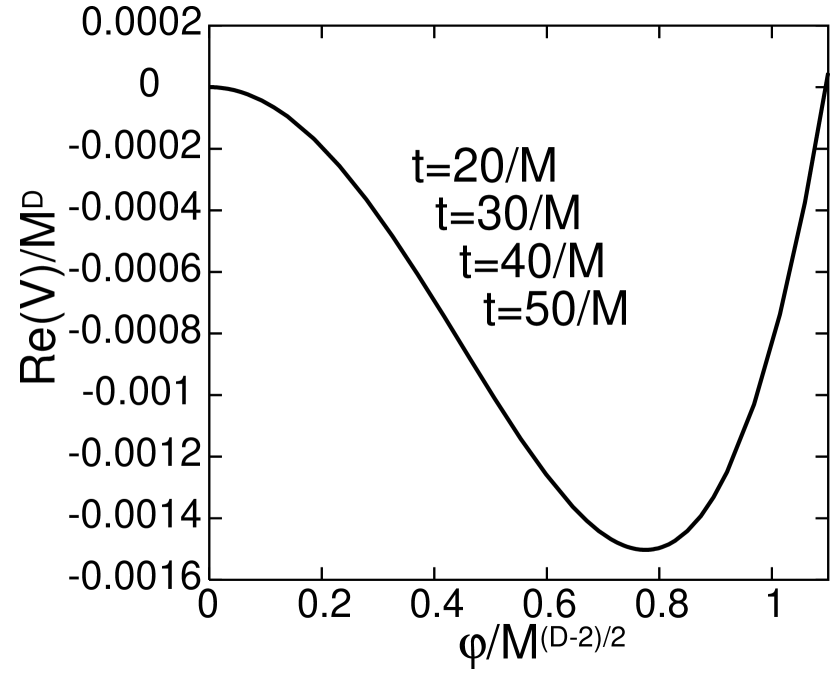
Figure 1: Behaviour of the effective potential and the mass gap for $\alpha=0$, $h_{0}=1$, $\xi=0$, $\mu_{r}=0.1M$, $\lambda=0.1M^{4-D}$ and $D=3.8$.

Figure 2: Behaviour of the effective potential and the mass gap for $\alpha=-1$, $h_{0}=1$, $\xi=0$, $\mu_{r}=0.1M$, $\lambda=0.1M^{4-D}$ and $D=3.8$.

Figure 3: Behaviour of the effective potential and the mass gap for $\alpha=1$, $h_{0}=1$, $\xi=0$, $\mu_{r}=0.1M$, $\lambda=0.1M^{4-D}$ and $D=3.8$.

We illustrate the behavior of the effective potential for a minimal gravitational coupling $\xi=0$ at $\mu_{r}=0.1M$ in Figs.1, 2 and 3. Here we set $D=3.8$ to regularize the theory with keeping the general covariance. It corresponds to the cut-off scale, $\Lambda\sim 500M_{2}$, where $M_{2}$ is a renormalization scale. Since the spacetime curvature behaves as $t^{-2}$, it raises up for a small $t$. It is not valid to apply the weak curvature expansion at the beginning of the universe. In Figs. 1, 2 and 3 we solve the gap equation only for $2<tM$. As is shown in the figures the effective potential seems to be almost proportional to $R^{\alpha}\propto t^{-2\alpha}$.

In Figs. 1 and 2 the expectation value $\langle\phi\rangle$ is located near the stationary point of the classical potential, $\displaystyle\phi^{2}=\frac{6}{\lambda}\mu_{r}^{2}$. For the minimal gravitational coupling the classical part of the effective action has no curvature dependence except for the overall factor and the Einstein-Hilbert term. On the other side, the radiative correction depends on the curvature. At $\alpha=0$ our model reduces to the ordinary $\phi^{4}$ theory. As is known, the radiative correction has only a small contribution to spontaneous symmetry breaking for a large $\mu_{r}$ in the ordinary theory. In the case of a negative $\alpha$ the classical part of the effective action (78) is enhanced as the curvature decreases. Contributions from the radiative corrections are lost at a large $t$. For a positive $\alpha$ the classical part of the effective action is suppressed except for the Einstein-Hilbert term as the curvature decreases. Hence we observe the curvature dependence of the expectation value $\langle\phi\rangle$ only if $\alpha>0$, see Fig. 3.

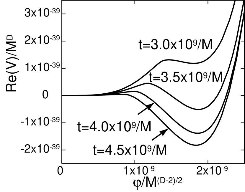
Figure 4: Behaviour of the effective potential and the mass gap for $\alpha=0$, $h_{0}=1$, $\xi=0$, $\mu_{r}=0$, $\lambda=0.1M^{4-D}$ and $D=3.8$.

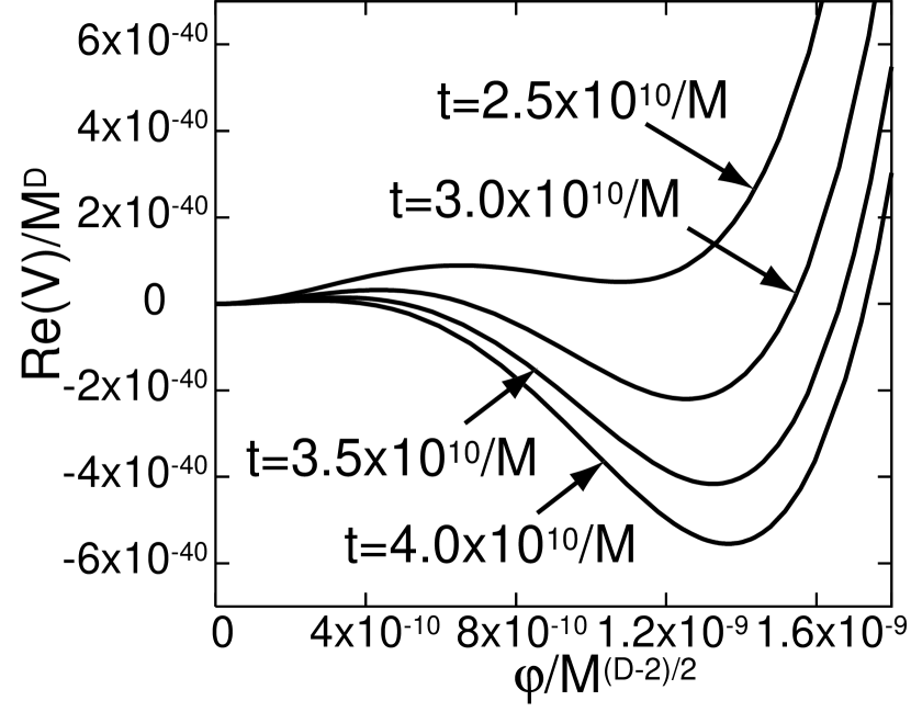
Figure 5: Behaviour of the effective potential and the mass gap for $\alpha=0$, $h_{0}=1$, $\xi=\xi_{\mbox{\scriptsize conformal}}$, $\mu_{r}=0$, $\lambda=0.1M^{4-D}$ and $D=3.8$.

Next we plot the behaviour of the effective potential for $\mu_{r}=0$ in Figs. 4, 5, 6 and 7. Here we consider the minimal and conformal gravitational coupling, $\xi=0$ and $\xi=\xi_{\mbox{\scriptsize conformal}}=(D-2)/[4(D-1)]$ respectively. (Of course, the scalar sector is conformally invariant for correspondent choice of $\xi$ only when $\alpha=0$.) For $\mu_{r}=0$ spontaneous symmetry breaking can not take place on the classical level of the ordinary $\phi^{4}$ theory. The radiative correction has an essential role to break the symmetry in the ordinary theory, i.e. $\alpha=0$. It is known as a radiative symmetry breaking. First order phase transition is observed in Figs. 4 and 5. However, the radiative correction has only a small effect. The expectation value generated by the radiative symmetry breaking is extremely small, as is shown in Figs. 4 and 5 at $\alpha=0$. A long time is necessary until phase transition takes place.

Figure 6: Behaviour of the effective potential and the mass gap for $\alpha=1$, $h_{0}=1$, $\xi=0$, $\mu_{r}=0$, $\lambda=0.1M^{4-D}$ and $D=3.8$.

Figure 7: Behaviour of the effective potential and the mass gap for $\alpha=1$, $h_{0}=1$, $\xi=\xi_{\mbox{\scriptsize conformal}}$, $\mu_{r}=0$, $\lambda=0.1M^{4-D}$ and $D=3.8$.

In the case of a positive $\alpha$ the ratio of the radiative correction to the classical part of the $\phi^{4}$ Lagrangian is enhanced as the curvature decreases. In Figs. 6 and 7 we also observe the first order phase transition and find that the expectation value $\langle\phi\rangle$ is extremely enhanced in comparison with the case $\alpha=0$. For $\alpha=-1$ only a symmetric phase is realized at $\mu_{r}=0$ and then radiative symmetry breaking does not occur.

As is shown in Figs. 6 and 7, the expectation value of $\phi$ has non-negligible time dependence for the case $\mu=0$. Hence we next consider the spacialy homogeneous but time dependent $\phi$ at $\mu=0$ and $\alpha=1$. Then we should solve the gap equation (19). From Eq. (19) the equation of motion for $\phi$ is obtained

$$\frac{1}{\sqrt{-g}}\frac{\delta}{\delta\phi}\int d^{D}x\sqrt{-g}{\cal L}_{eff}=-\frac{\partial V(\phi)}{\partial\phi}-\frac{1}{\sqrt{-g}}\partial_{\mu}\sqrt{-g}\left(\frac{R}{M^{2}}\right)^{\alpha}\partial^{\mu}\phi$$

$$=-\frac{\partial V(\phi)}{\partial\phi}-\left(\frac{R}{M^{2}}\right)^{\alpha}\left[\ddot{\phi}+(D-1)\frac{\dot{a}}{a}\dot{\phi}-\frac{2\alpha}{t}\dot{\phi}\right]=0.$$ (91)

To find an exact solution one needs to solve this equation for a general time-dependent form of $\phi$. However, it is instructive to consider the solution of Eq.(91) for a special form of $\phi$. In the present paper it is assumed that

$$\phi(t)=\langle\phi(t)\rangle=vt^{x},\ \ \phi^{;\mu}\phi_{;\mu}=\frac{x^{2}}{t^{2}}\langle\phi(t)\rangle^{2},$$ (92)

where $v$ is a constant parameter. Here we fix the parameter $x$ at $1/2$ or $1$ and numerically solve the equation of motion for $\phi$.

Under the assumption (92) Eq.(91) reads

$$\left[(x-1)+(D-1)h_{0}-2\alpha\right]\frac{x}{t^{2}}\phi(t)+\left(\frac{R}{M^{2}}\right)^{-\alpha}\frac{\partial V(\phi)}{\partial\phi}=0.$$ (93)

Thus the expectation value $\langle\phi\rangle$ is found by observing the stationary point of the following function

$$F[\phi]\equiv\left[(x-1)+(D-1)h_{0}-2\alpha\right]\frac{x}{2t^{2}}\phi(t)^{2}+\left(\frac{R}{M^{2}}\right)^{-\alpha}V(\phi).$$ (94)

The solution is shown in Figs. 8 and 9. As is seen in Figs. 8 and 9, we observe the first order phase transition again. In the case of the minimal gravitational coupling we find the two steps of the first order phase transition for $x=1$. In Fig. 8 (a) the solution becomes unstable for $tM<15.5$. The weak curvature approximation and/or the assumption $\langle\phi(t)\rangle=vt$ can not be applicable for such a small $t$. In all the cases the mass scale $v$ depends on the time $t$. However, we observe that the mass scale $v$ is almost static between $tM=80$ and $tM=90$ for $x=1$ and between $tM=90$ and $tM=100$ for $x=1/2$. It is expected that there is a solution with gradually decreasing $x$ after the first order phase transition near the time $tM=60$. On the other hand, we observe in Figs. 6, 7, 8 and 9 that the time of the first order transition near $tM=60$ has no large dependence on $x$ in the present analysis at $\alpha=1$ and $h_{0}=1$. It seems to be a characteristic feature of the theory with $\alpha=1$ in the FRW spacetime.

(a) $\langle\phi\rangle=v\sqrt{t},\ (x=1/2)$

(b) $\langle\phi\rangle=vt,\ (x=1)$

Figure 8: Behaviour of the mass scale $v$ for $\alpha=1$, $h_{0}=1$, $\xi=0$, $\mu_{r}=0$, $\lambda=0.1M^{4-D}$ and $D=3.8$.

(a) $\langle\phi\rangle=v\sqrt{t},\ (x=1/2)$

(b) $\langle\phi\rangle=vt,\ (x=1)$

Figure 9: Behaviour of the mass scale $v$ for $\alpha=1$, $h_{0}=1$, $\xi=\xi_{\mbox{\scriptsize conformal}}$, $\mu_{r}=0$, $\lambda=0.1M^{4-D}$ and $D=3.8$.

Hence, in the present section we numerically estimated phase structure for scalar theory in curved spacetime under consideration. The phase structure strongly depends on the sign of $\alpha$. Compared with the usual $\phi^{4}$ theory in weakly curved space, i.e. $\alpha=0$, a positive $\alpha$ significantly enhances the symmetry breaking. For a negative $\alpha$ the radiative symmetry breaking does not take place. As it was shown, mainly first-order curvature induced phase transitions may occur here.

In all figures we put $D=3.8$ and $h_{0}=1$. The spacetime curvature is given by Eq.(87) and found to be $R\sim 5.0/t^{2}$. The typical scale found to be $tM\sim 50$, $\langle\phi\rangle\sim 0.5M^{(D-2)/2}$ in Figs. 1$\sim$3, 6$\sim$9 and $tM\sim 10^{10}$, $\langle\phi\rangle\sim 10^{-9}M^{(D-2)/2}$ in Figs. 4, 5. The curvature scales for such time scales are given by $R\sim 0.002M^{2}$ and $10^{-20}M^{2}$ respectively. If we consider the electroweak scale Higgs boson, $\langle\phi\rangle\sim(100$GeV$)^{(D-2)/2}$, we obtain the typical mass scale $M\sim 200$GeV in the former case and $M\sim 10^{11}$GeV in the latter case. The cut-off scales which corresponds to $D=3.8$ are $\Lambda\sim 1$TeV, near the scale of a large extra dimension, and $10^{12}$GeV, respectively. For both cases the typical scale of time and curvature are given by $t\sim 0.1($GeV${}^{-1})$ and $R\sim 100($GeV${}^{2})$. Thus the quantum correction induced by the curvature effect has an interesting contribution to the effective action at the very early stage of the universe. The time scale of the phase transition depends on the coupling constant $\lambda$. For a stronger coupling the radiative correction is enhanced and a smaller time scale is obtained.

Thus we consider the regularized theory and calculate the effective potential in a D-dimensional spacetime with $D=3.8$. As is shown in the previous section, we obtain the finite effective potential (5) in four spacetime dimensions. Here we show some results in four dimensions. Evaluating the effective potential (5) we draw the solution of the gap equation. The first order phase transitions is observed as is shown in Fig. 10. Compared with the case $D=3.8$ (Figs. 6 and 7) the critical time becomes late and the the two steps transition does not realised in four dimensions.

(a) $\xi=0$

(b) $\xi=\xi_{\mbox{\scriptsize conformal}}$

Figure 10: Behaviour of the effective potential and the mass gap for $\alpha=1$, $h_{0}=1$, $\mu_{r}=0$, $\lambda=0.1$ in $D=4$.

The main lesson of this consideration is that it is unlikely that radiative corrections may strongly influence the dark energy universe in such theory. However, quantum effects may become quite important for phantom universe where Big Rip may occur [19, 20]. It was already demonstrated that in such circumstances already quantum effects of free fields may prevent Big Rip occurrence [21, 22, 23, 24]. However, in order to analyse this problem in our framework one needs the calculation of the one-loop effective action at strong curvature.

7 Dynamical mechanism to solve the cosmological constant problem

7.1 Dynamical cosmological constant theory: exact example

There are some proposals to solve the cosmological constant problem dynamically [2]. One of the possible solutions of the cosmological constant problem is pointed out by Mukohyama and Randall [3]. In [3], the following type of the action similar to the one under consideration has been proposed:

$$I=\int d^{4}x\sqrt{-g}\left[\frac{R}{2\kappa^{2}}+\alpha_{0}R^{2}+\frac{\left(\kappa^{4}\partial_{\mu}\varphi\partial^{\mu}\varphi\right)^{q}}{2q\kappa^{4}f(R)^{2q-1}}-V(\varphi)\right]\ ,$$ (95)

where $f(R)$ is a proper function of the scalar curvature $R$. When the curvature is small, it is assumed $f(R)$ behaves as

$$f(R)\sim\left(\kappa^{2}R^{2}\right)^{m}\ .$$ (96)

Here $m$ is positive. When the curvature is small, the vacuum energy, and therefore the value of the potential becomes small. Then one may assume, for the small curvature, $V(\varphi)$ behaves as

$$V(\varphi)\sim V_{0}\left(\varphi-\varphi_{c}\right)\ .$$ (97)

Here $V_{0}$ and $\varphi_{c}$ are constants. If $q>1/2$, the factor in front of the kinetic term of $\varphi$ in (95) becomes large. This makes the time development of the scalar field $\varphi$ very slow and it is expected that $\varphi$ does not reach $\varphi_{c}$. This model may explain the acceleration of the present universe. The model (95) is also expected to be stable under the radiative corrections. In fact, when the curvature is small and the time development of the curvature can be neglected, if we rescale the scalar field $\varphi$ as $\varphi\to R^{m(2q-1)/q}\varphi$, the curvature in the kinetic term can be absorbed into the redefinition of $\varphi$ and there appear factors including $R^{m(2q-1)/q}$. Therefore if $m(2q-1)/q>0$, the interactions could be suppressed when the curvature is small and there will not appear the radiative correction to the vacuum energy except the one loop corrections.

We now show that there is an exactly solvable model, which realizes the scenario in [3]. Assume $m=q=1$ and (96) and (97) are exact:

$$f(R)=\beta R^{2}\ ,\quad V(\varphi)=V_{0}\left(\varphi-\varphi_{c}\right)\ .$$ (98)

Here $\beta$ is a constant. $R^{2}$ term is neglected by putting $\alpha_{0}=0$ in (95) since the curvature is small. Then by the variation over the metric, one obtains

$$0 = -\frac{1}{2}\left\{\frac{R}{2\kappa^{2}}+\frac{\partial_{\rho}\varphi\partial^{\rho}\varphi}{2\beta R^{2}}-V_{0}\left(\varphi-\varphi_{c}\right)\right\}g_{\mu\nu}+\frac{R_{\mu\nu}}{2\kappa^{2}}-\frac{\partial_{\rho}\varphi\partial^{\rho}\varphi R_{\mu\nu}}{\beta R^{3}}$$ (99)

$$+\frac{\partial_{\mu}\varphi\partial_{\nu}\varphi}{2\beta R^{2}}-\left(\nabla_{\mu}\nabla_{\nu}-g_{\mu\nu}\nabla^{2}\right)\left(\frac{\partial_{\rho}\varphi\partial^{\rho}\varphi}{\beta R^{3}}\right)\ .$$

On the other hand, the variation over $\varphi$ gives

$$0=-\partial_{\mu}\left(\sqrt{-g}\frac{\partial^{\mu}\varphi}{\beta R^{2}}\right)-V_{0}\sqrt{-g}\ .$$ (100)

We assume the four dimensional FRW metric with flat spatial part:

$$ds^{2}=dt^{2}-a(t)^{2}\sum_{i=1,2,3}\left(dx^{i}\right)^{2}\ .$$ (101)

It is chosen that $\varphi$ only depends on the time coordinate $t$. Then the $(t,t)$-component of (99) gives

$$0 = -\frac{3H^{2}}{2\kappa^{2}}+\frac{{\dot{\varphi}}^{2}}{144\beta\left(\dot{H}+H^{2}\right)^{2}}+V_{0}\left(\varphi-\varphi_{c}\right)$$ (102)

$$+H\frac{d}{dt}\left(\frac{{\dot{\varphi}}^{2}}{12\beta\left(\dot{H}+H^{2}\right)^{2}}\right)-\frac{{\dot{\varphi}}^{2}\left(\dot{H}+H^{2}\right)}{72\beta\left(\dot{H}+H^{2}\right)^{3}}\ ,$$

where $H$ is the Hubble rate. On the other hand, (100) gives

$$0=-\frac{d}{dt}\left(\frac{a^{3}\dot{\varphi}}{36\beta\left(\dot{H}+H^{2}\right)^{2}}\right)-V_{0}a^{3}\ .$$ (103)

A solution of Eqs.(102) and (103) is given by

$$a=a_{0}t^{h_{0}}\ \left(H=\frac{h_{0}}{t}\right)\ ,\quad\varphi=\varphi_{c}+\frac{\varphi_{0}}{t^{2}}\ ,$$ (104)

when $h_{0}>0$. In case $h_{0}<0$, this scale factor $a=a_{0}t^{h_{0}}$ (104) does not express expanding universe but shrinking one. If the direction of time is changed as $t\to-t$, the expanding universe emerges with scale factor $a=a_{0}(-t)^{h_{0}}$. In the expression, however, since $h_{0}$ is not always an integer, $t$ should be negative so that the scale factor should be real. To avoid this apparent difficulty, we may further shift the origin of the time as $t\to-t\to t_{s}-t$. Then the time $t$ can be positive as long as $t<t_{s}$. When $h_{0}<0$, instead of (104), one may propose

$$a=a_{0}\left(t_{s}-t\right)^{h_{0}}\ \left(H=\frac{h_{0}}{t_{s}-t}\right)\ ,\quad\varphi=\varphi_{c}+\frac{\varphi_{0}}{\left(t_{s}-t\right)^{2}}\ ,$$ (105)

The assumption (104) or (105) reduces Eqs.(102) and (103) to the algebraic equations:

$$0 = -\frac{3h_{0}^{2}}{2\kappa^{2}}+\frac{\varphi_{0}^{2}h_{0}}{36\beta\left(-h_{0}+2h_{0}^{2}\right)^{3}}+V_{0}\varphi_{0}\ ,$$ (106)

$$0 = \frac{\varphi_{0}\left(3h_{0}+1\right)}{18\beta\left(-h_{0}+2h_{0}^{2}\right)^{2}}-V_{0}\ ,$$ (107)

which gives

$$\varphi_{0}^{2} = \frac{54\beta\left(-1+2h_{0}\right)^{3}h_{0}^{4}}{\kappa^{2}\left(12h_{0}^{2}-2h_{0}-1\right)}\ ,$$

$$V_{0} = \pm\frac{3h_{0}+1}{\sqrt{6\kappa^{2}\left(12h_{0}^{2}-2h_{0}-1\right)\left(-1+2h_{0}\right)}}\ .$$ (108)

Since $\varphi_{0}^{2}$ should be positive, one finds

$$\mbox{when}\ \beta>0\ ,\quad \frac{1-\sqrt{13}}{12}<h_{0}<\frac{1+\sqrt{13}}{12}\ \mbox{or}\ h_{0}\geq\frac{1}{2}\ ,$$ (109)

$$\mbox{when}\ \beta<0\ ,\quad h_{0}<\frac{1-\sqrt{13}}{12}\ \mbox{or}\ \frac{1+\sqrt{13}}{12}<h_{0}\leq\frac{1}{2}\ .$$

By properly choosing the parameter $\beta$ and $V_{0}$, we can always obtain a solution as in (104) or (105). For example, if

$$h_{0}=-\frac{1}{60}\ ,$$ (110)

which gives the following value of the parameter $w$ of the equation of state

$$w=-1+\frac{2}{3h_{0}}=-1.025\ ,$$ (111)

we find

$$\kappa V_{0}=\pm\frac{19}{34}\sqrt{\frac{15}{31}}=\pm 0.388722...\ .$$ (112)

It is interesting that the value of $w$ (111) is consistent with the observed one.

For $h_{0}>0$ case, corresponding to (104), since $R=6\dot{H}+12H^{2}$, the curvature $R$ decreases as $t^{-2}$ with time $t$. Eq.(104) tells that $\varphi$ approaches to $\varphi_{c}$ but does not arrive at $\varphi_{c}$ in a finite time, as expected in [3].

As seen from the expression of $H$ in (104) or (105), if we substitute the value of the age of the present universe $10^{10}$years$\sim(10^{-33}$eV$)^{-1}$ into $t$ or $t_{s}-t$, the observed value of $H$ could be reproduced, which could explain the smallness of the effective cosmological constant $\Lambda\sim H^{2}$. Note that even if there is no potential term, that is, $V_{0}=0$, when $\beta<0$, there is a solution

$$h_{0}=-\frac{1}{3}<\frac{1-\sqrt{13}}{12}=-0.2171...\ ,$$ (113)

which gives the parameter $w$ of the equation of state: $w=-3$, although $w$ is not realistic.

7.2 Cosmological constant problem in scalar theory non-linearly coupled with curvature

Here we consider the solution of the cosmological constant problem in the theory (1). As is shown in the previous section, one could expect that the radiative correction is suppressed when the curvature is small if $\alpha<0$. As in the case of (95), if we rescale $\phi$ by $\phi\to(R/M^{2})^{-\alpha/2}\phi$, the kinetic term becomes standardly normalized one and does not include the curvature. The $\phi^{4}$ interaction terms, however, include the factor $(R/M^{2})^{-\alpha}$ and may be suppressed for the small curvature. Hence, there would not appear the radiative correction to the vacuum energy except the one-loop corrections.

As an example of the solvable case, we put $\alpha=-1$ and $\mu_{0}^{2}=0$. The variation over the metric gives

$$0 = -\frac{1}{2}\left[\frac{R}{2\kappa^{2}}-\frac{M^{2}}{R}\left\{\frac{1}{2}\partial_{\rho}\phi\partial^{\rho}\phi-\frac{\xi R}{2}\phi^{2}+\frac{\lambda}{4!}\phi^{4}\right\}\right]g_{\mu\nu}+\frac{R_{\mu\nu}}{2\kappa^{2}}$$ (114)

$$+\frac{M^{2}}{2R}\partial_{\mu}\phi\partial_{\nu}\phi-\frac{M^{2}R_{\mu\nu}}{R^{2}}\left\{\frac{1}{2}\partial_{\rho}\phi\partial^{\rho}\phi+\frac{\lambda}{4!}\phi^{4}\right\}$$

$$-\left(\nabla_{\mu}\nabla_{\nu}-g_{\mu\nu}\nabla^{2}\right)\left\{\frac{M^{2}}{R^{2}}\left(\frac{1}{2}\partial_{\rho}\phi\partial^{\rho}\phi+\frac{\lambda}{4!}\phi^{4}\right)\right\}\ .$$

Scalar field equation is

$$0=-\frac{1}{\sqrt{-g}}\partial_{\mu}\left(\sqrt{-g}\frac{\partial^{\mu}\phi}{R}\right)+\frac{\lambda}{3!R}\phi^{3}+\xi\phi\ .$$ (115)

By assuming the FRW metric (101) and $\phi=\phi(t)$, Eqs.(114) and (115) have the following forms:

$$0 = -\frac{3H^{2}}{2\kappa^{2}}+\frac{M^{2}\left(\frac{1}{2}{\dot{\phi}}^{2}-\frac{\lambda}{4!}\phi^{4}\right)}{12\left(\dot{H}+2H^{2}\right)}-\frac{M^{2}\left(\dot{H}+H^{2}\right)\left(\frac{1}{2}{\dot{\phi}}^{2}+\frac{\lambda}{4!}\phi^{4}\right)}{12\left(\dot{H}+2H^{2}\right)^{2}}$$ (116)

$$+\frac{M^{2}\xi}{4}\phi^{2}-\frac{M^{2}}{12}\frac{d}{dt}\left(\frac{\left(\frac{1}{2}{\dot{\phi}}^{2}+\frac{\lambda}{4!}\phi^{4}\right)}{\left(\dot{H}+2H^{2}\right)^{2}}\right)\ ,$$

$$0 = -\frac{d}{dt}\left(\frac{a^{3}\dot{\phi}}{\dot{H}+2H^{2}}\right)+\frac{\lambda a^{3}\phi^{3}}{3!\left(\dot{H}+2H^{2}\right)}+\xi\phi a^{3}\ .$$ (117)

With the Anzats

$$H=\frac{h_{0}}{t}\ ,\quad\phi=\frac{\phi_{0}}{t}\ ,$$ (118)

when $h_{0}>0$ or

$$H=\frac{h_{0}}{t_{s}-t}\ ,\quad\phi=\frac{\phi_{0}}{t_{s}-t}\ ,$$ (119)

when $h_{0}<0$. Eqs.(116) and (117) reduce to the algebraic equations:

$$0 = -\frac{3h_{0}^{2}}{2\kappa^{2}}+\frac{M^{2}}{12\left(-h_{0}+2h_{0}^{2}\right)}\left(\frac{1}{2}\phi_{0}^{2}-\frac{\lambda}{4!}\phi_{0}^{4}\right)$$ (120)

$$-\frac{M^{2}\left(-h_{0}+h_{0}^{2}\right)}{12\left(-h_{0}+2h_{0}^{2}\right)^{2}}\left(\frac{1}{2}\phi_{0}^{2}+\frac{\lambda}{4!}\phi_{0}^{4}\right)+\frac{M^{2}\xi}{4}\phi_{0}^{2}\ ,$$

$$0 = \frac{h_{0}\phi_{0}}{2\left(-h_{0}+2h_{0}^{2}\right)}+\frac{\lambda\phi_{0}^{3}}{36\left(-h_{0}+h_{0}^{2}\right)}+\xi\phi_{0}\ ,$$ (121)

which give

$$\phi_{0}^{2} = \frac{3}{\displaystyle\kappa^{2}\left\{\frac{8-9h_{0}}{24\left(-h_{0}+h_{0}^{2}\right)^{2}}-\frac{\left(4-7h_{0}\right)\xi}{\left(-h_{0}+2h_{0}^{2}\right)h_{0}}\right\}}\ ,$$ (122)

$$\lambda = -6\kappa^{2}h_{0}\left\{1-2\left(1-2h_{0}\right)\xi\right\}$$ (123)

$$\times\left\{\frac{8-9h_{0}}{24\left(-h_{0}+h_{0}^{2}\right)^{2}}-\frac{\left(4-7h_{0}\right)\xi}{\left(-h_{0}+2h_{0}^{2}\right)h_{0}}\right\}\ .$$

Therefore, with the proper choice of parameters, the solution in the form of (118) or (119) follows. We should note the behavior of $H$ (118) or (119) is almost identical with that in (104) or (105).

One may consider the model including two scalar fields $\varphi$ and $\phi$ as

$$I = \int d^{4}x\sqrt{-g}\left[\frac{R}{2\kappa^{2}}+\frac{\partial_{\mu}\varphi\partial^{\mu}\varphi}{2\beta R^{2}}-V_{0}\left(\varphi-\varphi_{c}\right)\right.$$ (124)

$$\left.-\frac{M^{2}}{R}\left\{\frac{1}{2}\partial_{\mu}\phi\partial^{\mu}\phi+\frac{\xi R}{2}\phi^{2}+\frac{\lambda}{4!}\phi^{4}\right\}\right]\ .$$

Even in this case, for FRW metric (101) and assuming (104) or (105) and/or (118) or (119), we obtain (117) and (121). The equation corresponding to (116) and/or (120) has the following form:

$$0 = -\frac{3H^{2}}{2\kappa^{2}}+\frac{M^{2}\left(\frac{1}{2}{\dot{\phi}}^{2}-\frac{\lambda}{4!}\phi^{4}\right)}{12\left(\dot{H}+2H^{2}\right)}-\frac{M^{2}\left(\dot{H}+H^{2}\right)\left(\frac{1}{2}{\dot{\phi}}^{2}+\frac{\lambda}{4!}\phi^{4}\right)}{12\left(\dot{H}+2H^{2}\right)^{2}}$$ (125)

$$+\frac{M^{2}\xi}{4}\phi^{2}-\frac{M^{2}}{12}\frac{d}{dt}\left(\frac{\left(\frac{1}{2}{\dot{\phi}}^{2}+\frac{\lambda}{4!}\phi^{4}\right)}{\left(\dot{H}+2H^{2}\right)^{2}}\right)$$

$$+\frac{M^{2}}{12\left(-h_{0}+2h_{0}^{2}\right)}\left(\frac{1}{2}\phi_{0}^{2}-\frac{\lambda}{4!}\phi_{0}^{4}\right)$$

$$-\frac{M^{2}\left(-h_{0}+h_{0}^{2}\right)}{12\left(-h_{0}+2h_{0}^{2}\right)^{2}}\left(\frac{1}{2}\phi_{0}^{2}+\frac{\lambda}{4!}\phi_{0}^{4}\right)+\frac{M^{2}\xi}{4}\phi_{0}^{2}\ .$$

Then by properly choosing the parameters, we may obtain an exact solution for cosmological constant again.

Hence, we demonstrated that the mechanism proposed in ref.[3] to dynamically solve the cosmological constant problem is naturally realized also for the class of models investigated in this work.

The final remark is in order. In [25] (see also [26]), the cosmological constant damping in the model contained $\phi^{2}R$ term in the Lagrangian has been investigated. It has been shown the possibility to solve the cosmological constant problem. Although the problem could be solved in the model, the effective Newton constant $G_{\rm eff}$ suffers the correction like $G_{\rm eff}\sim G_{0}/\left(1+a\phi^{2}\right)$ with a constant $a$. Here $G_{0}$ is the bare Newton constant. In the solution of model [25], $\phi$ behaves as a linear function of the time $t$. Naturally $t$ could be the age of the present universe, $t\sim\left(10^{-33}\,\mbox{eV}\right)^{-1}$, the correction becomes very large and the effective Newton constant becomes unnaturally small. In the model under consideration (1) with (2), similar term is included but due to the factor $R^{\alpha}$, if $\alpha>0$, the correction is suppressed since $R\sim\left(10^{-33}\,\mbox{eV}\right)^{2}$ and $R$ is very small. In general $\alpha$ can be also negative. In the solvable case in (114), the correction could be $R^{-2}\left\{\frac{1}{2}\partial_{\rho}\phi\partial^{\rho}\phi+\frac{\lambda}{4!}\phi^{4}\right\}$. Since the $R\sim t^{-2}$ or $\left(t_{s}-t\right)^{-2}$, by combining (118) or (119), the correction takes the order of unity. Then the effective Newton constant could receive the correction but it is finite, which does not lead to the instabilities of the above sort (smallness of gravitational constant).

8 Conclusion

In summary, we studied the scalar self-interacting theory whose Lagrangian non-linearly couples with some power of the curvature as the effective field theory. The one-loop effective action at weak curvature is found here using specific regularization scheme. The phase structure of the theory is carefully investigated, the examples of curvature-induced phase transitions are presented numerically (for the case of positive power of curvature). The comparison with the ordinary scalar self-interacting theory in curved space is done. For negative value of $\alpha$ the radiative symmetry breaking does not take place. It remains to develop the same one-loop formulation at strong curvature as in such a case the phase transitions maybe considered in the vicinity of Big Rip.

The dynamical mechanism to explain the origin of the extremely small cosmological constant in the spirit of papers [2, 3] is presented. It is shown that in the class of the models under consideration (including the case with two scalars) such a proposal maybe realized quite successfully. Unfortunately, despite the preliminary expectations the radiative corrections for the theory under consideration are not relevant in the study of the dynamical cosmological constant.

There are many directions where our approach maybe generalised. In particularly, it is known that phase structure of NJL model in curved spacetime is quite rich (for a review, see [27]). Hence, it would be extremely interesting to consider the NJL-like models non-linearly coupled with power of the curvature in the same spirit. Such models maybe even more attractive due to fact that $1/N$ expansion is more reliable than one-loop approximation in non-renormalizable theories. One can also consider Yang-Mills theory (or Born-Infeld theory) coupled to curvature powers in the same way. Definitely, this may bring the number of the interesting applications in such issues as dark energy and cosmological constant.

From another point, the new matter-gravity coupling [1] maybe also considered as kind of modification of gravitation itself. In such a situation, when theory somehow deviates from General Relativity, it is not clear apriori if the metric formalism and first-order formulation should lead to the same physical picture [28]. (Indeed, unlike to General Relativity where metric and Palatini formulations basically coincide, it is not the case for our theory (1)[1] already on classical level [29]). It would be extremely interesting to develop the one-loop effective action formulation in the same way as the one developed in this paper when an external gravity is formulated in Palatini form. This will be done elsewhere.

References

References

- [1] Nojiri S and Odintsov S D 2004 Phys. Lett.B 599 137
- [2] Dolgov A D and Kawasaki M 2003 Preprint astro-ph/0307442
- [3] Mukohyama S and Randall L 2004 Phys. Rev. Lett.92 211302
- [4] Jackiw R, Nunez C and Pi S -Y 2005 Preprint hep-th/0502215 (to appear in the Einstein Memorial Issue of Phys. Lett.A)
- [5] Buchbinder I L, Odintsov S D and Shapiro I L 1992 Effective Action in Quantum Gravity (IOP Publishing)
- [6] Birrell N D and Davies P C 1982 Quantum Fields in Curved Space (Cambridge University Press)
- [7] Abdalla M C B, Nojiri S and Odintsov S D 2005 Class. Quantum Grav.22 L35
- [8] Bunch T S and Parker L 1979 Phys. Rev.D 20 2499
- [9] Parker L and Toms D J 1984 Phys. Rev.D 29 1584
- [10] Petrov A Z 1969 Einstein Space, (Pergamon, Oxford)
- [11] Elizalde E, Odintsov S D, Romeo A, Bytsenko A and Zerbini S 1994 Zeta- Regularization with Applications (Singapore: World Scientific)
- [12] Shore G M 1980 Ann. Phys., Lpz.128 376
- [13] Allen R 1983 Nucl. Phys.B226 228
- [14] Ishikawa K 1983 Phys. Rev.D 28 2445
- [15] Hu B L and O’Connor D J 1984 Phys. Rev.D 30 743
- [16] Buchbinder I L and Odintsov S D 1985 Class. Quantum Grav.2 721
- [17] Odintsov S D 1993 Phys. Lett.B 306 233
- [18] Odintsov S D 1991 Fortschritte der Physik 39 621
- [19] Caldwell R, Kamionkowski M and Weinberg N 2003 Phys. Rev. Lett.91 071301
- [20] McInnes B 2002 J. High Energy Phys. JHEP0208(2002)029
- [21] Nojiri S and Odintsov S D 2004 Phys. Lett.B 595 1
- [22] Nojiri S and Odintsov S D 2004 Phys. Rev.D 70 10352
- [23] Elizalde E, Nojiri S and Odintsov S D 2004 Phys. Rev.D 70 043539
- [24] Nojiri S, Odintsov S D and Tsujikawa S 2005 Preprint hep-th/0501025
- [25] Dolgov A D 1982 in “The very early universe” Eds. Gibbobs G, Hawking S W, and Siklos S T, Cambridge University Press, p.449
- [26] Ford L H 1987 Phys. Rev. D35 2339
- [27] Inagaki T, Muta T and Odintsov S D 1997 Prog. Theor. Phys. Suppl. 127 93
- [28] Ferravis M, Francaviglia M and Volovich I 1994 Class. Quantum Grav.11 1505
- [29] Allemandi G, Borowiec A, Francaviglia M and Odintsov S D 2005 Preprint gr-qc/0504057