The basics of gravitational wave theory

Abstract

Einstein’s special theory of relativity revolutionized physics by teaching us that space and time are not separate entities, but join as “spacetime”. His general theory of relativity further taught us that spacetime is not just a stage on which dynamics takes place, but is a participant: The field equation of general relativity connects matter dynamics to the curvature of spacetime. Curvature is responsible for gravity, carrying us beyond the Newtonian conception of gravity that had been in place for the previous two and a half centuries. Much research in gravitation since then has explored and clarified the consequences of this revolution; the notion of dynamical spacetime is now firmly established in the toolkit of modern physics. Indeed, this notion is so well established that we may now contemplate using spacetime as a tool for other science. One aspect of dynamical spacetime — its radiative character, “gravitational radiation” — will inaugurate entirely new techniques for observing violent astrophysical processes. Over the next one hundred years, much of this subject’s excitement will come from learning how to exploit spacetime as a tool for astronomy. This article is intended as a tutorial in the basics of gravitational radiation physics.

1 Introduction: Spacetime and gravitational waves

Einstein’s special relativity [1] taught us that space and time are not simply abstract, external concepts, but must in fact be considered measured observables, like any other quantity in physics. This reformulation enforced the philosophy that Newton sought to introduce in laying out his laws of mechanics [2]:

$\ldots$ I frame no hypotheses; for whatever is not reduced from the phenomena is to be called an hypothesis; and hypotheses $\ldots$ have no place in experimental philosophy $\ldots$

Despite his intention to stick only with that which can be observed, Newton described space and time using exactly the abstract notions that he otherwise deplored [3]:

Absolute space, in its own nature, without relation to anything external, remains always similar and immovable

Absolute, true, and mathematical time, of itself, and from its own nature, flows equably without relation to anything external.

Special relativity put an end to these abstractions: Time is nothing more than that which is measured by clocks, and space is that which is measured by rulers. The properties of space and time thus depend on the properties of clocks and rulers. The constancy of the speed of light as measured by observers in different reference frames, as observed in the Michelson-Morley experiment, forces us inevitably to the fact that space and time are mixed into spacetime. Ten years after his paper on special relativity, Einstein endowed spacetime with curvature and made it dynamical [5]. This provided a covariant theory of gravity [6], in which all predictions for physical measurements are invariant under changes in coordinates. In this theory, general relativity, the notion of “gravitational force” is reinterpreted in terms of the behavior of geodesics in the curved manifold of spacetime.

To be compatible with special relativity, gravity must be causal: Any change to a gravitating source must be communicated to distant observers no faster than the speed of light, $c$. This leads immediately to the idea that there must exist some notion of “gravitational radiation”. As demonstrated by Bernard Schutz, one can actually calculate with surprising accuracy many of the properties of gravitational radiation simply by combining a time dependent Newtonian potential with special relativity [7].

The first calculation of gravitational radiation in general relativity is due to Einstein. His initial calculation [8] was “marred by an error in calculation” (Einstein’s words), and was corrected in 1918 [9] (albeit with an overall factor of two error). Modulo a somewhat convoluted history (discussed in great detail by Kennefick [10]) owing (largely) to the difficulties of analyzing radiation in a nonlinear theory, Einstein’s final result stands today as the leading-order “quadrupole formula” for gravitational wave emission. This formula plays a role in gravity theory analogous to the dipole formula for electromagnetic radiation, showing that gravitational waves (hereafter abbreviated GWs) arise from accelerated masses exactly as electromagnetic waves arise from accelerated charges.

The quadrupole formula tells us that GWs are difficult to produce — very large masses moving at relativistic speeds are needed. This follows from the weakness of the gravitational interaction. A consequence of this is that it is extremely unlikely there will ever be an interesting laboratory source of GWs. The only objects massive and relativistic enough to generate detectable GWs are astrophysical. Indeed, experimental confirmation of the existence of GWs has come from the study of binary neutron star systems — the variation of the mass quadrupole in such systems is large enough that GW emission changes the system’s characteristics on a timescale short enough to be observed. The most celebrated example is the “Hulse-Taylor” pulsar, B1913+16, reported by Russell Hulse and Joe Taylor in 1975 [11]. Thirty years of observation have shown that the orbit is decaying; the results match with extraordinary precision general relativity’s prediction for such a decay due to the loss of orbital energy and angular momentum by GWs. For a summary of the most recent data, see Ref. [12], Fig. 1. Hulse and Taylor were awarded the Nobel Prize for this discovery in 1993. Since this pioneering system was discovered, several other double neutron star systems “tight” enough to exhibit strong GW emission have been discovered [13, 14, 15, 16].

Studies of these systems prove beyond a reasonable doubt that GWs exist. What remains is to detect the waves directly and exploit them — to use GWs as a way to study astrophysical objects. The contribution to this volume by Danzmann [21] discusses the challenges and program of directly measuring these waves. Intuitively, it is clear that measuring these waves must be difficult — the weakness of the gravitational interaction ensures that the response of any detector to gravitational waves is very small. Nonetheless, technology has brought us to the point where detectors are now beginning to set interesting upper limits on GWs from some sources [17, 18, 19, 20]. First direct detection is now hopefully not too far in the future.

The real excitement will come when detection becomes routine. We will then have an opportunity to retool the “physics experiment” of direct detection into the development of astronomical observatories. Some of the articles appearing in this volume will discuss likely future revolutions which, at least conceptually, should change our notions of spacetime in a manner as fundamental as Einstein’s works in 1905 and 1915 (see, e.g., papers by Ashtekar and Horowitz). Such a revolution is unlikely to be driven by GW observations — most of what we expect to learn using GWs will apply to regions of spacetime that are well-described using classical general relativity; it is highly unlikely that Einstein’s theory will need major revisions prompted by GW observations. Any revolution arising from GW science will instead be in astrophysics: Mature GW measurements have the potential to study regions of the Universe that are currently inaccessible to our instruments. During the next century of spacetime study, spacetime will itself be exploited to study our Universe.

1.1 Why this article?

As GW detectors have improved and approached maturity, many articles have been written reviewing this field and its promise. One might ask: Do we really need another one? As partial answer to this question, we note that Richard Price requested this article very nicely. More seriously, our goal is to provide a brief tutorial on the basics of GW science, rather than a comprehensive survey of the field. The reader who is interested in such a survey can find such in Refs. [22, 23, 24, 25, 26, 27, 28, 29, 30]. Other reviews on the basics of GW science can be found in Refs. [31, 32]; we also recommend the dedicated conference procedings [33, 34, 35].

We assume that the reader has a basic familiarity with general relativity, at least at the level of Hartle’s textbook [36]; thus, we assume the reader understands metrics and is reasonably comfortable taking covariant derivatives. We adapt what Baumgarte and Shapiro [37] call the “Fortran convention” for indices: $a,b,c\ldots h$ denote spacetime indices which run over $0,1,2,3$ or $t,x,y,z$, while $i,j,k\ldots n$ denote spatial indices which run over $1,2,3$. We use the Einstein summation convention throughout — repeated adjacent indices in the “upstairs” and “downstairs” positions imply a sum:

$$u^{a}v_{a}\equiv\sum_{a}u^{a}v_{a}\;.$$

When we discuss linearized theory, we will sometimes be sloppy and sum over adjacent spatial indices in the same position. Hence,

$$u_{i}v_{i}\equiv u^{i}v^{i}\equiv u^{i}v_{i}\equiv\sum_{i}u^{i}v_{i}$$

is valid in linearized theory. (As we will discuss in Sec. 2, this is allowable because, in linearized theory, the position of a spatial index is immaterial in Cartesian coordinates.) A quantity that is symmetrized on pairs of indices is written

$$A_{(ab)}=\frac{1}{2}\left(A_{ab}+A_{ba}\right)\;.$$

Throughout most of this article we use “relativist’s units”, in which $G=1=c$; mass, space, and time have the same units in this system. The following conversion factors are often useful for converting to “normal” units:

$$1\,\mbox{second} = 299,792,458\,\mbox{meters}\simeq 3\times 10^{8}\,\mbox{meters}$$

$$1\,M_{\odot} = 1476.63\,\mbox{meters}\simeq 1.5\,\mbox{kilometers}$$

$$= 4.92549\times 10^{-6}\,\mbox{seconds}\simeq 5\,\mbox{microseconds}\;.$$

($1\,M_{\odot}$ is one solar mass.) We occasionally restore factors of $G$ and $c$ to write certain formulae in normal units.

Section 2 provides an introduction to linearized gravity, deriving the most basic properties of GWs. Our treatment in this section is mostly standard. One aspect of our treatment that is slightly unusual is that we introduce a gauge-invariant formalism that fully characterizes the linearized gravity’s degrees of freedom. We demonstrate that the linearized Einstein equations can be written as 5 Poisson-type equations for certain combinations of the spacetime metric, plus a wave equation for the transverse-traceless components of the metric perturbation. This analysis helps to clarify which degrees of freedom in general relativity are radiative and which are not, a useful exercise for understanding spacetime dynamics.

Section 3 analyses the interaction of GWs with detectors whose sizes are small compared to the wavelength of the GWs. This includes ground-based interferometric and resonant-mass detectors, but excludes space-based interferometric detectors. The analysis is carried out in two different gauges; identical results are obtained from both analyses. Section 4 derives the leading-order formula for radiation from slowly-moving, weakly self-gravitating sources, the quadrupole formula discussed above.

In Sec. 5, we develop linearized theory on a curved background spacetime. Many of the results of “basic linearized theory” (Sec. 2) carry over with slight modification. We introduce the “geometric optics” limit in this section, and sketch the derivation of the Isaacson stress-energy tensor, demonstrating how GWs carry energy and curve spacetime. Section 6 provides a very brief synopsis of GW astronomy, leading the reader through a quick tour of the relevant frequency bands and anticipated sources. We conclude by discussing very briefly some topics that we could not cover in this article, with pointers to good reviews.

2 The basic basics: Gravitational waves in linearized gravity

The most natural starting point for any discussion of GWs is linearized gravity. Linearized gravity is an adequate approximation to general relativity when the spacetime metric, $g_{ab}$, may be treated as deviating only slightly from a flat metric, $\eta_{ab}$:

$$g_{ab}=\eta_{ab}+h_{ab},\qquad||h_{ab}||\ll 1\;.$$ (2.1)

Here $\eta_{ab}$ is defined to be $\mbox{diag}(-1,1,1,1)$ and $||h_{ab}||$ means “the magnitude of a typical non-zero component of $h_{ab}$”. Note that the condition $||h_{ab}||\ll 1$ requires both the gravitational field to be weak, and in addition constrains the coordinate system to be approximately Cartesian. We will refer to $h_{ab}$ as the metric perturbation; as we will see, it encapsulates GWs, but contains additional, non-radiative degrees of freedom as well. In linearized gravity, the smallness of the perturbation means that we only keep terms which are linear in $h_{ab}$ — higher order terms are discarded. As a consequence, indices are raised and lowered using the flat metric $\eta_{ab}$. The metric perturbation $h_{ab}$ transforms as a tensor under Lorentz transformations, but not under general coordinate transformations.

We now compute all the quantities which are needed to describe linearized gravity. The components of the affine connection (Christoffel coefficients) are given by

$${\Gamma^{a}}_{bc} = \frac{1}{2}\eta^{ad}\left(\partial_{c}h_{db}+\partial_{b}h_{dc}-\partial_{d}h_{bc}\right)$$ (2.2)

$$= \frac{1}{2}\left(\partial_{c}{h^{a}}_{b}+\partial_{b}{h^{a}}_{c}-\partial^{a}h_{bc}\right)\;.$$

Here $\partial_{a}$ means the partial derivative $\partial/\partial x^{a}$. Since we use $\eta_{ab}$ to raise and lower indices, spatial indices can be written either in the “up” position or the “down” position without changing the value of a quantity: $f^{x}=f_{x}$. Raising or lowering a time index, by contrast, switches sign: $f^{t}=-f_{t}$. The Riemann tensor we construct in linearized theory is then given by

$$R^{a}_{\ bcd} = \partial_{c}{\Gamma^{a}}_{bd}-\partial_{d}{\Gamma^{a}}_{bc}$$ (2.3)

$$= \frac{1}{2}\left(\partial_{c}\partial_{b}{h^{a}}_{d}+\partial_{d}\partial^{a}h_{bc}-\partial_{c}\partial^{a}h_{bd}-\partial_{d}\partial_{b}{h^{a}}_{c}\right)\;.$$

From this, we construct the Ricci tensor

$$R_{ab}={R^{c}}_{acb}=\frac{1}{2}\left(\partial_{c}\partial_{b}{h^{c}}_{a}+\partial^{c}\partial_{a}h_{bc}-\Box h_{ab}-\partial_{a}\partial_{b}h\right)\;,$$ (2.4)

where $h={h^{a}}_{a}$ is the trace of the metric perturbation, and $\Box=\partial_{c}\partial^{c}=\nabla^{2}-\partial_{t}^{2}$ is the wave operator. Contracting once more, we find the curvature scalar:

$$R={R^{a}}_{a}=\left(\partial_{c}\partial^{a}{h^{c}}_{a}-\Box h\right)$$ (2.5)

and finally build the Einstein tensor:

$$G_{ab} = R_{ab}-\frac{1}{2}\eta_{ab}R$$ (2.6)

$$= \frac{1}{2}\left(\partial_{c}\partial_{b}{h^{c}}_{a}+\partial^{c}\partial_{a}h_{bc}-\Box h_{ab}-\partial_{a}\partial_{b}h\right.$$

$$\qquad\left.-\eta_{ab}\partial_{c}\partial^{d}{h^{c}}_{d}+\eta_{ab}\Box h\right)\;.$$

This expression is a bit unwieldy. Somewhat remarkably, it can be cleaned up significantly by changing notation: Rather than working with the metric perturbation $h_{ab}$, we use the trace-reversed perturbation $\bar{h}_{ab}=h_{ab}-\frac{1}{2}\eta_{ab}h$. (Notice that $\bar{h^{a}}_{a}=-h$, hence the name “trace reversed”.) Replacing $h_{ab}$ with $\bar{h}_{ab}+\frac{1}{2}\eta_{ab}h$ in Eq. (2.6) and expanding, we find that all terms with the trace $h$ are canceled. What remains is

$$G_{ab}=\frac{1}{2}\left(\partial_{c}\partial_{b}{{\bar{h}}^{c}}_{\ a}+\partial^{c}\partial_{a}\bar{h}_{bc}-\Box\bar{h}_{ab}-\eta_{ab}\partial_{c}\partial^{d}{{\bar{h}}^{c}}_{\ d}\right)\;.$$ (2.7)

This expression can be simplified further by choosing an appropriate coordinate system, or gauge. Gauge transformations in general relativity are just coordinate transformations. A general infinitesimal coordinate transformation can be written as ${x^{a}}^{\prime}=x^{a}+\xi^{a}$, where $\xi^{a}(x^{b})$ is an arbitrary infinitesimal vector field. This transformation changes the metric via

$$h_{ab}^{\prime}=h_{ab}-2\partial_{(a}\xi_{b)}\;,$$ (2.8)

so that the trace-reversed metric becomes

$$\bar{h}_{ab}^{\prime} = h_{ab}^{\prime}-\frac{1}{2}\eta_{ab}h^{\prime}$$ (2.9)

$$= \bar{h}_{ab}-2\partial_{(b}\xi_{a)}+\eta_{ab}\partial^{c}\xi_{c}\;.$$

A class of gauges that are commonly used in studies of radiation are those satisfying the Lorentz gauge condition

$$\partial^{a}\bar{h}_{ab}=0\;.$$ (2.10)

(Note the close analogy to Lorentz gauge in electromagnetic theory, $\partial^{a}A_{a}=0$, where $A_{a}$ is the potential vector.)

Suppose that our metric perturbation is not in Lorentz gauge. What properties must $\xi_{a}$ satisfy in order to impose Lorentz gauge? Our goal is to find a new metric $h^{\prime}_{ab}$ such that $\partial^{a}\bar{h}^{\prime}_{ab}=0$:

$$\partial^{a}\bar{h}_{ab}^{\prime} = \partial^{a}\bar{h}_{ab}-\partial^{a}\partial_{b}\xi_{a}-\Box\xi_{b}+\partial_{b}\partial^{c}\xi_{c}$$ (2.11)

$$= \partial^{a}\bar{h}_{ab}-\Box\xi_{b}\;.$$ (2.12)

Any metric perturbation $h_{ab}$ can therefore be put into a Lorentz gauge by making an infinitesimal coordinate transformation that satisfies

$$\Box\xi_{b}=\partial^{a}\bar{h}_{ab}\;.$$ (2.13)

One can always find solutions to the wave equation (2.13), thus achieving Lorentz gauge. The amount of gauge freedom has now been reduced from 4 freely specifiable functions of 4 variables to 4 functions of 4 variables that satisfy the homogeneous wave equation $\Box\xi^{b}=0$, or, equivalently, to 8 freely specifiable functions of 3 variables on an initial data hypersurface.

Applying the Lorentz gauge condition (2.10) to the expression (2.7) for the Einstein tensor, we find that all but one term vanishes:

$$G_{ab}=-\frac{1}{2}\Box\bar{h}_{ab}\;.$$ (2.14)

Thus, in Lorentz gauges, the Einstein tensor simply reduces to the wave operator acting on the trace reversed metric perturbation (up to a factor $-1/2$). The linearized Einstein equation is therefore

$$\Box\bar{h}_{ab}=-16\pi T_{ab}\;;$$ (2.15)

in vacuum, this reduces to

$$\Box\bar{h}_{ab}=0\;.$$ (2.16)

Just as in electromagnetism, the equation (2.15) admits a class of homogeneous solutions which are superpositions of plane waves:

$${\bar{h}}_{ab}({\bf x},t)={\rm Re}\int d^{3}k\ A_{ab}({\bf k})e^{i({\bf k}\cdot{\bf x}-\omega t)}\;.$$ (2.17)

Here, $\omega=|{\bf k}|$. The complex coefficients $A_{ab}({\bf k})$ depend on the wavevector ${\bf k}$ but are independent of ${\bf x}$ and $t$. They are subject to the constraint $k^{a}A_{ab}=0$ (which follows from the Lorentz gauge condition), with $k^{a}=(\omega,{\bf k})$, but are otherwise arbitrary. These solutions are gravitational waves.

2.1 Globally vacuum spacetimes: Transverse traceless (TT) gauge

We now specialize to globally vacuum spacetimes in which $T_{ab}=0$ everywhere, and which are asymptotically flat (for our purposes, $h_{ab}\to 0$ as $r\to\infty$). Equivalently, we specialize to the space of homogeneous, asymptotically flat solutions of the linearized Einstein equation (2.15). For such spacetimes one can, along with choosing Lorentz gauge, further specialize the gauge to make the metric perturbation be purely spatial

$$h_{tt}=h_{ti}=0$$ (2.18)

and traceless

$$h=h_{i}^{\ i}=0.$$ (2.19)

The Lorentz gauge condition (2.10) then implies that the spatial metric perturbation is transverse:

$$\partial_{i}h_{ij}=0.$$ (2.20)

This is called the transverse-traceless gauge, or TT gauge. A metric perturbation that has been put into TT gauge will be written $h_{ab}^{\rm TT}$. Since it is traceless, there is no distinction between $h^{\rm TT}_{ab}$ and $\bar{h}^{\rm TT}_{ab}$.

The conditions (2.18) and (2.19) comprise 5 constraints on the metric, while the residual gauge freedom in Lorentz gauge is parameterized by 4 functions that satisfy the wave equation. It is nevertheless possible to satisfy these conditions, essentially because the metric perturbation satisfies the linearized vacuum Einstein equation. When the TT gauge conditions are satisfied the gauge is completely fixed.

One might wonder why we would choose TT gauge. It is certainly not necessary; however, it is extremely convenient, since the TT gauge conditions completely fix all the local gauge freedom. The metric perturbation $h_{ab}^{\rm TT}$ therefore contains only physical, non-gauge information about the radiation. In TT gauge there is a close relation between the metric perturbation and the linearized Riemann tensor $R_{abcd}$ [which is invariant under the local gauge transformations (2.8) by Eq. (2.3)], namely

$$R_{itjt}=-\frac{1}{2}{\ddot{h}}_{ij}^{\rm TT}.$$ (2.21)

In a globally vacuum spacetime, all non-zero components of the Riemann tensor can be obtained from $R_{itjt}$ via Riemann’s symmetries and the Bianchi identity. In a more general spacetime, there will be components that are not related to radiation; this point is discussed further in Sec. 2.2.

Transverse traceless gauge also exhibits the fact that gravitational waves have two polarization components. For example, consider a GW which propagates in the $z$ direction: $h^{\rm TT}_{ij}=h^{\rm TT}_{ij}(t-z)$ is a valid solution to the wave equation $\Box h^{\rm TT}_{ij}=0$. The Lorentz condition $\partial_{z}h^{\rm TT}_{zj}=0$ implies that $h^{\rm TT}_{zj}(t-z)=\mbox{constant}$. This constant must be zero to satisfy the condition that $h_{ab}\to 0$ as $r\to\infty$. The only non-zero components of $h^{\rm TT}_{ij}$ are then $h^{\rm TT}_{xx}$, $h^{\rm TT}_{xy}$, $h^{\rm TT}_{yx}$, and $h^{\rm TT}_{yy}$. Symmetry and the tracefree condition (2.19) further mandate that only two of these are independent:

$$h^{\rm TT}_{xx} = -h^{\rm TT}_{yy}\equiv h_{+}(t-z)\;;$$ (2.22)

$$h^{\rm TT}_{xy} = h^{\rm TT}_{yx}\equiv h_{\times}(t-z)\;.$$ (2.23)

The quantities $h_{+}$ and $h_{\times}$ are the two independent waveforms of the GW (see Fig. 1).

For globally vacuum spacetimes, one can always satisfy the TT gauge conditions. To see this, note that the most general gauge transformation $\xi^{a}$ that preserves the Lorentz gauge condition (2.10) satisfies $\Box\xi^{a}=0$, from Eq. (2.12). The general solution to this equation can be written

$$\xi^{a}={\rm Re}\int d^{3}k\ C^{a}({\bf k})e^{i({\bf k}\cdot{\bf x}-\omega t)}$$ (2.24)

for some coefficients $C^{a}({\bf k})$. Under this transformation the tensor $A_{ab}({\bf k})$ in Eq. (2.17) transforms as

$$A_{ab}\to A^{\prime}_{ab}=A_{ab}-2ik_{(a}C_{b)}+i\eta_{ab}k^{d}C_{d}\;.$$ (2.25)

Achieving the TT gauge conditions (2.20) and (2.19) therefore requires finding, for each ${\bf k}$, a $C^{a}({\bf k})$ that satisfies the two equations

$$0 = \eta^{ab}A^{\prime}_{ab}=\eta^{ab}A_{ab}+2ik^{a}C_{a}$$ (2.26)

$$\mbox{}0 = A^{\prime}_{tb}=A_{tb}-iC_{b}k_{t}-iC_{t}k_{b}+i{\delta^{t}}_{b}(k^{a}C_{a})\;;$$ (2.27)

${\delta^{t}}_{b}$ is the Kronecker delta — zero for $b\neq t$, unity otherwise. An explicit solution to these equations is given by

$$C_{a}=\frac{3A_{bc}l^{b}l^{c}}{8i\omega^{4}}k_{a}+\frac{\eta^{bc}A_{bc}}{4i\omega^{4}}l_{a}+\frac{1}{2i\omega^{2}}A_{ab}l^{b}\;,$$ (2.28)

where $k^{a}=(\omega,{\bf k})$ and $l^{a}=(\omega,-{\bf k})$.

2.2 Global spacetimes with matter sources

We now return to the more general and realistic situation in which the stress-energy tensor is non-zero. We continue to assume that the linearized Einstein equations are valid everywhere in spacetime, and that we consider asymptotically flat solutions only. In this context, the metric perturbation $h_{ab}$ contains (i) gauge degrees of freedom; (ii) physical, radiative degrees of freedom; and (iii) physical, non-radiative degrees of freedom tied to the matter sources. Because of the presence of the physical, non-radiative degrees of freedom, it is not possible in general to write the metric perturbation in TT gauge. However, the metric perturbation can be split up uniquely into various pieces that correspond to the degrees of freedom (i), (ii) and (iii), and the radiative degrees of freedom correspond to a piece of the metric perturbation that satisfies the TT gauge conditions, the so-called TT piece.

This aspect of linearized theory is obscured by the standard, Lorentz gauge formulation (2.15) of the linearized Einstein equations. There, all the components of $h_{ab}$ appear to be radiative, since all the components obey wave equations. In this subsection, we describe a formulation of linearized theory which focuses on gauge invariant observables. In particular, we will see that only the TT part of the metric obeys a wave equation in all gauges. We show that the non-TT parts of the metric can be gathered into a set of gauge invariant functions; these functions are governed by Poisson equations rather than wave equations. This shows that the non-TT pieces of the metric do not exhibit radiative degrees of freedom. Although one can always choose gauges like Lorentz gauge in which the non-radiative parts of the metric obey wave equations and thus appear to be radiative, this appearance is gauge artifact. Such gauge choices, although useful for calculations, can cause one to mistake purely gauge modes for truly physical radiation.

Interestingly, the first analysis contrasting physical radiative degrees of freedom from purely coordinate modes appears to have been performed by Eddington in 1922 [40]. Eddington was somewhat suspicious of Einstein’s analysis [9], as Einstein chose a gauge in which all metric functions propagated with the speed of light. Though the entire metric appeared to be radiative (by construction), Einstein found that only the “transverse-transverse” pieces of the metric carried energy. Eddington wrote:

Weyl has classified plane gravitational waves into three types, viz. (1) longitudinal-longitudinal; (2) longitudinal-transverse; (3) transverse-trans-verse. The present investigation leads to the conclusion that transverse-transverse waves are propagated with the speed of light in all systems of co-ordinates. Waves of the first and second types have no fixed velocity — a result which rouses suspicion as to their objective existence. Einstein had also become suspicious of these waves (in so far as they occur in his special co-ordinate system) for another reason, because he found that they convey no energy. They are not objective, and (like absolute velocity) are not detectable by any conceivable experiment. They are merely sinuosities in the co-ordinate system, and the only speed of propagation relevant to them is “the speed of thought.”

$\ldots$ It is evidently a great convenience in analysis to have all waves, both physical and spurious, travelling with one velocity; but it is liable to obscure physical ideas by mixing them up so completely. The chief new point in the present discussion is that when unrestricted co-ordinates are allowed the genuine waves continue to travel with the velocity of light and the spurious waves cease to have any fixed velocity.

Unfortunately, Eddington’s wry dismissal of unphysical modes as propagating with “the speed of thought” is often taken by skeptics (and crackpots) as applying to all gravitational perturbations. Eddington in fact showed quite the opposite. We do so now using somewhat more modern notation; our presentation is essentially the flat-spacetime limit of Bardeen’s [41] gauge-invariant cosmological perturbation formalism. A similar treatment can be found in lecture notes by Bertschinger [42].

We begin by defining the decomposition of the metric perturbation $h_{ab}$, in any gauge, into a number of irreducible pieces. Assuming that $h_{ab}\to 0$ as $r\to\infty$, we define the quantities $\phi$, $\beta_{i}$, $\gamma$, $H$, $\varepsilon_{i}$, $\lambda$ and $h_{ij}^{\rm TT}$ via the equations

$$h_{tt} = 2\phi\;,$$ (2.29)

$$h_{ti} = \beta_{i}+\partial_{i}\gamma\;,$$ (2.30)

$$h_{ij} = h_{ij}^{\rm TT}+\frac{1}{3}H\delta_{ij}+\partial_{(i}\varepsilon_{j)}+\left(\partial_{i}\partial_{j}-\frac{1}{3}\delta_{ij}\nabla^{2}\right)\lambda\;,$$ (2.31)

together with the constraints

$$\partial_{i}\beta_{i} = 0\quad\mbox{(1 constraint)}$$ (2.32)

$$\partial_{i}\varepsilon_{i} = 0\quad\mbox{(1 constraint)}$$ (2.33)

$$\partial_{i}h_{ij}^{\rm TT} = 0\quad\mbox{(3 constraints)}$$ (2.34)

$$\delta^{ij}h_{ij}^{\rm TT} = 0\quad\mbox{(1 constraint)}$$ (2.35)

and boundary conditions

$$\gamma\to 0,\ \ \ \varepsilon_{i}\to 0,\ \ \ \lambda\to 0,\ \ \ \nabla^{2}\lambda\to 0$$ (2.36)

as $r\to\infty$. Here $H\equiv\delta^{ij}h_{ij}$ is the trace of the spatial portion of the metric perturbation, not to be confused with the spacetime trace $h=\eta^{ab}h_{ab}$ that we used earlier. The spatial tensor $h_{ij}^{\rm TT}$ is transverse and traceless, and is the TT piece of the metric discussed above which contains the physical radiative degrees of freedom. The quantities $\beta_{i}$ and $\partial_{i}\gamma$ are the transverse and longitudinal pieces of $h_{ti}$. The uniqueness of this decomposition follows from taking a divergence of Eq. (2.30) giving $\nabla^{2}\gamma=\partial_{i}h_{ti}$, which has a unique solution by the boundary condition (2.36). Similarly, taking two derivatives of Eq. (2.31) yields the equation $2\nabla^{2}\nabla^{2}\lambda=3\partial_{i}\partial_{j}h_{ij}-\nabla^{2}H$, which has a unique solution by Eq. (2.36). Having solved for $\lambda$, one can obtain a unique $\varepsilon_{i}$ by solving $3\nabla^{2}\varepsilon_{i}=6\partial_{j}h_{ij}-2\partial_{i}H-4\partial_{i}\nabla^{2}\lambda$.

The total number of free functions in the parameterization (2.29) – (2.31) of the metric is 16: 4 scalars ($\phi$, $\gamma$, $H$, and $\lambda$), 6 vector components ($\beta_{i}$ and $\varepsilon_{i}$), and 6 symmetric tensor components ($h_{ij}^{\rm TT}$). The number of constraints (2.32) – (2.35) is 6, so the number of independent variables in the parameterization is 10, consistent with a symmetric $4\times 4$ tensor.

We next discuss how the variables $\phi$, $\beta_{i}$, $\gamma$, $H$, $\varepsilon_{i}$, $\lambda$ and $h_{ij}^{\rm TT}$ transform under gauge transformations $\xi^{a}$ with $\xi^{a}\to 0$ as $r\to\infty$. We parameterize such gauge transformation as

$$\xi_{a}=(\xi_{t},\xi_{i})\equiv(A,B_{i}+\partial_{i}C)\;,$$ (2.37)

where $\partial_{i}B_{i}=0$ and $C\to 0$ as $r\to\infty$; thus $B_{i}$ and $\partial_{i}C$ are the transverse and longitudinal pieces of the spatial gauge transformation. The transformed metric is $h_{ab}-2\partial_{(a}\xi_{b)}$; decomposing this transformed metric into its irreducible pieces yields the transformation laws

$$\phi \to \quad\phi-\dot{A}\;,$$ (2.38)

$$\beta_{i} \to \quad\beta_{i}-\dot{B}_{i}\;,$$ (2.39)

$$\gamma \to \quad\gamma-A-\dot{C}\;,$$ (2.40)

$$H \to \quad H-2\nabla^{2}C\;,$$ (2.41)

$$\lambda \to \quad\lambda-2C\;,$$ (2.42)

$$\varepsilon_{i} \to \quad\varepsilon_{i}-2B_{i}\;,$$ (2.43)

$$h_{ij}^{\rm TT} \to \quad h_{ij}^{\rm TT}\;.$$ (2.44)

Gathering terms, we see that the following combinations of these functions are gauge invariant:

$$\Phi \equiv -\phi+\dot{\gamma}-\frac{1}{2}\ddot{\lambda}\;,$$ (2.45)

$$\Theta \equiv \frac{1}{3}\left(H-\nabla^{2}\lambda\right)\;,$$ (2.46)

$$\Xi_{i} \equiv \beta_{i}-\frac{1}{2}\dot{\varepsilon}_{i}\;;$$ (2.47)

$h_{ij}^{\rm TT}$ is gauge-invariant without any further manipulation. In the Newtonian limit $\Phi$ reduces to the Newtonian potential $\Phi_{N}$, while $\Theta=-2\Phi_{N}$. The total number of free, gauge-invariant functions is 6: 1 function $\Theta$; 1 function $\Phi$; 3 functions $\Xi_{i}$, minus 1 due to the constraint $\partial_{i}\Xi_{i}=0$; and 6 functions $h_{ij}^{\rm TT}$, minus 3 due to the constraints $\partial_{i}h_{ij}^{\rm TT}=0$, minus 1 due to the constraint $\delta^{ij}h_{ij}^{\rm TT}=0$. This is in keeping with the fact that in general the 10 metric functions contain 6 physical and 4 gauge degrees of freedom.

We would now like to enforce Einstein’s equation. Before doing so, it is useful to first decompose the stress energy tensor in a manner similar to that of our decomposition of the metric. We define the quantities $\rho$, $S_{i}$, $S$, $P$, $\sigma_{ij}$, $\sigma_{i}$ and $\sigma$ via the equations

$$T_{tt} = \rho\;,$$ (2.48)

$$T_{ti} = S_{i}+\partial_{i}S\;,$$ (2.49)

$$T_{ij} = P\delta_{ij}+\sigma_{ij}+\partial_{(i}\sigma_{j)}+\left(\partial_{i}\partial_{j}-\frac{1}{3}\delta_{ij}\nabla^{2}\right)\sigma,\;$$ (2.50)

together with the constraints

$$\partial_{i}S_{i} = 0\;,$$ (2.51)

$$\partial_{i}\sigma_{i} = 0\;,$$ (2.52)

$$\partial_{i}\sigma_{ij} = 0\;,$$ (2.53)

$$\delta^{ij}\sigma_{ij} = 0,\;$$ (2.54)

and boundary conditions

$$S\to 0,\ \ \ \sigma_{i}\to 0,\ \ \ \sigma\to 0,\ \ \ \nabla^{2}\sigma\to 0$$ (2.55)

as $r\to\infty$. These quantities are not all independent. The variables $\rho$, $P$, $S_{i}$ and $\sigma_{ij}$ can be specified arbitrarily; stress-energy conservation ($\partial^{a}T_{ab}=0$) then determines the remaining variables $S$, $\sigma$, and $\sigma_{i}$ via

$$\nabla^{2}S = \dot{\rho}\;,$$ (2.56)

$$\nabla^{2}\sigma = -\frac{3}{2}P+\frac{3}{2}\dot{S}\;,$$ (2.57)

$$\nabla^{2}\sigma_{i} = 2\dot{S}_{i}\;.$$ (2.58)

We now compute the Einstein tensor from the metric (2.29) – (2.31). The result can be expressed in terms of the gauge invariant observables:

$$G_{tt} = -\nabla^{2}\Theta\;,$$ (2.59)

$$G_{ti} = -\frac{1}{2}\nabla^{2}\Xi_{i}-\partial_{i}\dot{\Theta}\;,$$ (2.60)

$$G_{ij} = -\frac{1}{2}\Box h_{ij}^{\rm TT}-\partial_{(i}\dot{\Xi}_{j)}-\frac{1}{2}\partial_{i}\partial_{j}\left(2\Phi+\Theta\right)$$

$$\qquad+\delta_{ij}\left[\frac{1}{2}\nabla^{2}\left(2\Phi+\Theta\right)-\ddot{\Theta}\right]\;.$$

We finally enforce Einstein’s equation $G_{ab}=8\pi T_{ab}$ and simplify using the conservation relations (2.56) – (2.58); this leads to the following field equations:

$$\nabla^{2}\Theta = -8\pi\rho\;,$$ (2.62)

$$\nabla^{2}\Phi = 4\pi\left(\rho+3P-3\dot{S}\right)\;,$$ (2.63)

$$\nabla^{2}\Xi_{i} = -16\pi S_{i}\;,$$ (2.64)

$$\Box h_{ij}^{\rm TT} = -16\pi\sigma_{ij}\;.$$ (2.65)

Notice that only the metric components $h_{ij}^{\rm TT}$ obey a wave-like equation. The other variables $\Theta$, $\Phi$ and $\Xi_{i}$ are determined by Poisson-type equations. Indeed, in a purely vacuum spacetime, the field equations reduce to five Laplace equations and a wave equation:

$$\nabla^{2}\Theta^{\rm vac} = 0\;,$$ (2.66)

$$\nabla^{2}\Phi^{\rm vac} = 0\;,$$ (2.67)

$$\nabla^{2}\Xi_{i}^{\rm vac} = 0\;,$$ (2.68)

$$\Box h_{ij}^{\rm TT,vac} = 0\;.$$ (2.69)

This manifestly demonstrates that only the $h_{ij}^{\rm TT}$ metric components — the transverse, traceless degrees of freedom of the metric perturbation — characterize the radiative degrees of freedom in the spacetime. Although it is possible to pick a gauge in which other metric components appear to be radiative, they will not be: Their radiative character is an illusion arising due to the choice of gauge or coordinates.

The field equations (2.62) – (2.65) also demonstrate that, far from a dynamic, radiating source, the time-varying portion of the physical degrees of freedom in the metric is dominated by $h_{ij}^{\rm TT}$. If we expand the gauge invariant fields $\Phi$, $\Theta$, $\Xi_{i}$ and $h_{ij}^{\rm TT}$ in powers of $1/r$, then, at sufficiently large distances, the leading-order $O(1/r)$ terms will dominate. For the fields $\Theta$, $\Phi$ and $\Xi_{i}$, the coefficients of the $1/r$ pieces are simply the conserved mass $\int d^{3}x\rho$ or the conserved linear momentum $-\int d^{3}xS_{i}$, from the conservation relations (2.56) – (2.58). Thus, the only time-varying piece of the physical degrees of freedom in the metric perturbation at order $O(1/r)$ is the TT piece $h_{ij}^{\rm TT}$. An alternative proof of this result is given in Exercise 19.1 of Misner, Thorne and Wheeler [4].

Although the variables $\Phi$, $\Theta$, $\Xi_{i}$ and $h_{ij}^{\rm TT}$ have the advantage of being gauge invariant, they have the disadvantage of being non-local. Computation of these variables at a point requires knowledge of the metric perturbation $h_{ab}$ everywhere. This non-locality obscures the fact that the physical, non-radiative degrees of freedom are causal, a fact which is explicit in Lorentz gauge . On the other hand, many observations that seek to detect GWs are sensitive only to the value of the Riemann tensor at a given point in space (see Sec. 3). For example, the Riemann tensor components $R_{itjt}$, which are directly observable by detectors such as LIGO, are given in terms of the gauge invariant variables as

$$R_{itjt}=-\frac{1}{2}{\ddot{h}}_{ij}^{\rm TT}+\Phi_{,ij}+{\dot{\Xi}}_{(i,j)}-\frac{1}{2}{\ddot{\Theta}}\delta_{ij}.$$ (2.70)

Thus, at least certain combinations of the gauge invariant variables are locally observable.

2.3 Local regions of spacetime

In the previous subsection we described a splitting of metric perturbations into radiative, non-radiative, and gauge pieces. This splitting requires that the linearized Einstein equations be valid throughout the spacetime. However, this assumption is not valid in the real Universe: Many sources of GWs are intrinsically strong field sources and cannot be described using linearized theory, and on cosmological scales the metric of our Universe is not close to the Minkowski metric. Furthermore the splitting requires a knowledge of the metric throughout all of spacetime, whereas any measurements or observations can probe only finite regions of spacetime. For these reasons it is useful to consider linearized perturbation theory in finite regions of spacetime, and to try to define gravitational radiation in this more general context.

Consider therefore a finite volume ${\cal V}$ in space. Can we split up the metric perturbation $h_{ab}$ in ${\cal V}$ into radiative and non-radiative pieces? In general, the answer is no: Within any finite region GWs cannot be distinguished from time-varying near-zone fields generated by sources outside that region. One way to see this is to note that in finite regions of space, the decomposition of the metric into various pieces becomes non-unique, as does the decomposition of vectors into transverse and longitudinal pieces. [For example the vector $(x^{2}-y^{2})\partial_{z}$ is both transverse and longitudinal.] Alternatively, we note that within any finite vacuum region ${\cal V}$, one can always find a gauge which is locally TT, that is, a gauge which satisfies the conditions (2.18) – (2.20) within the region. (This fact does not seem to be widely known, so we give a proof in A). In particular, this applies to the static Coulomb-type field of a point source, as long as the source itself is outside of ${\cal V}$. Consequently, isolating the TT piece of the metric perturbation does not yield just the radiative degrees of freedom within a local region – a TT metric perturbation may also contain, for example, Coulomb-type fields.

Within finite regions of space, therefore, GWs cannot be defined at a fundamental level – one simply has time-varying gravitational fields. However, there is a certain limit in which GWs can be approximately defined in local regions, namely the limit in which the wavelength of the waves is much smaller than length and time scales characterizing the background metric. This definition of gravitational radiation is discussed in detail and in a more general context in Sec. 5. As discussed in that section, this limit will always be valid when one is sufficiently far from all radiating sources.

3 Interaction of gravitational waves with a detector

The usual notion of “gravitational force” disappears in general relativity, replaced instead by the idea that freely falling bodies follow geodesics in spacetime. Given a spacetime metric $g_{ab}$ and a set of spacetime coordinates $x^{a}$, geodesic trajectories are given by the equation

$$\frac{d^{2}x^{a}}{d\tau^{2}}+{\Gamma^{a}}_{bc}\frac{dx^{b}}{d\tau}\frac{dx^{c}}{d\tau}=0\;,$$ (3.1)

where $\tau$ is proper time as measured by an observer travelling along the geodesic. By writing the derivatives in the geodesic equation (3.1) in terms of coordinate time $t$ rather than proper time $\tau$, and by combining the $a=t$ equation with the spatial, $a=j$ equations, we obtain an equation for the coordinate acceleration:

$$\frac{d^{2}x^{i}}{dt^{2}}=-(\Gamma^{i}_{tt}+2\Gamma^{i}_{tj}v^{j}+\Gamma^{i}_{jk}v^{j}v^{k})+v^{i}(\Gamma^{t}_{tt}+2\Gamma^{t}_{tj}v^{j}+\Gamma^{t}_{jk}v^{j}v^{k}),$$ (3.2)

where $v^{i}=dx^{i}/dt$ is the coordinate velocity.

Let us now specialize to linearized theory, with the non-flat part of our metric dominated by a GW in TT gauge. Further, let us specialize to non-relativistic motion for our test body. This implies that $v^{i}\ll 1$, and to a good approximation we can neglect the velocity dependent terms in Eq. (3.2):

$$\frac{d^{2}x^{i}}{dt^{2}}+{\Gamma^{i}}_{tt}=0\;.$$ (3.3)

In linearized theory and TT gauge,

$${\Gamma^{i}}_{tt}=\Gamma_{itt}=\frac{1}{2}\left(2\partial_{t}h^{\rm TT}_{jt}-\partial_{j}h^{\rm TT}_{tt}\right)=0$$ (3.4)

since $h^{\rm TT}_{at}=0$. Hence, we find that $d^{2}x^{i}/dt^{2}=0$.

Does this result mean that the GW has no effect? Certainly not! It just tells us that in TT gauge the coordinate location of a slowly moving, freely falling body is unaffected by the GW. In essence, the coordinates move with the waves.

This result illustrates why, in general relativity, it is important to focus upon coordinate-invariant observables — a naive interpretation of the above result would be that freely falling bodies are not influenced by GWs. In fact the GWs cause the proper separation between two freely falling particles to oscillate, even if the coordinate separation is constant. Consider two spatial freely falling particles, located at $z=0$, and separated on the $x$ axis by a coordinate distance $L_{c}$. Consider a GW in TT gauge that propagates down the $z$ axis, $h^{\rm TT}_{ab}(t,z)$. The proper distance $L$ between the two particles in the presence of the GW is given by

$$L = \int_{0}^{L_{c}}dx\,\sqrt{g_{xx}}=\int_{0}^{L_{c}}dx\,\sqrt{1+h^{\rm TT}_{xx}(t,z=0)}$$ (3.5)

$$\simeq \int_{0}^{L_{c}}dx\,\left[1+\frac{1}{2}h^{\rm TT}_{xx}(t,z=0)\right]=L_{c}\left[1+\frac{1}{2}h^{\rm TT}_{xx}(t,z=0)\right]\;.$$

Notice that we use the fact that the coordinate location of each particle is fixed in TT gauge! In a gauge in which the particles move with respect to the coordinates, the limits of integration would have to vary. Equation (3.5) tells us that the proper separation of the two particles oscillates with a fractional length change $\delta L/L$ given by

$$\frac{\delta L}{L}\simeq\frac{1}{2}h^{\rm TT}_{xx}(t,z=0)\;.$$ (3.6)

Although we used TT gauge to perform this calculation, the result is gauge independent; we will derive it in a different gauge momentarily. Notice that $h^{\rm TT}_{xx}$ acts as a strain — a fractional length change. The magnitude $h$ of a wave is often referred to as the “wave strain”. The proper distance we have calculated here is a particularly important quantity since it directly relates to the accumulated phase which is measured by laser interferometric GW observatories (cf. the contribution by Danzmann in this volume). The “extra” phase $\delta\phi$ accumulated by a photon that travels down and back the arm of a laser interferometer in the presence of a GW is $\delta\phi=4\pi\delta L/\lambda$, where $\lambda$ is the photon’s wavelength and $\delta L$ is the distance the end mirror moves relative to the beam splitter. We now give a different derivation of the fractional length change (3.6) based on the concept of geodesic deviation. Consider a geodesic in spacetime given by $x^{a}=z^{a}(\tau)$, where $\tau$ is the proper time, with four velocity $u^{a}(\tau)=dz^{a}/d\tau$. Suppose we have a nearby geodesic $x^{a}(\tau)=z^{a}(\tau)+L^{a}(\tau)$, where $L^{a}(\tau)$ is small. We can regard the coordinate displacement $L^{a}$ as a vector ${\vec{L}}=L^{a}\partial_{a}$ on the first geodesic; this is valid to first order in ${\vec{L}}$. Without loss of generality, we can make the connecting vector be purely spatial: $L^{a}u_{a}=0$. Spacetime curvature causes the separation vector to change with time — the geodesics will move further apart or closer together, with an acceleration given by the geodesic deviation equation

$$u^{b}\nabla_{b}(u^{c}\nabla_{c}L^{a})=-{R^{a}}_{bcd}[{\vec{z}}(\tau)]u^{b}L^{c}u^{d}\;;$$ (3.7)

see, e.g., Ref. [36], Chap. 21. This equation is valid to linear order in $L^{a}$; fractional corrections to this equation will scale as $L/{\cal L}$, where ${\cal L}$ is the lengthscale over which the curvature varies.

For application to GW detectors, the shortest such lengthscale ${\cal L}$ is the wavelength $\lambda$ of the GWs. Thus, the geodesic deviation equation will have fractional corrections of order $L/\lambda$. For ground-based detectors $L\;\hbox to0.0pt{\lower 2.5pt\hbox{$\sim$}\hss}\raise 1.5pt\hbox{$<$}\;$ a few km, while $\lambda\;\hbox to0.0pt{\lower 2.5pt\hbox{$\sim$}\hss}\raise 1.5pt\hbox{$>$}\;3000{\rm km}$ (see Sec. 6.1); thus the approximation will be valid. For detectors with $L\;\hbox to0.0pt{\lower 2.5pt\hbox{$\sim$}\hss}\raise 1.5pt\hbox{$>$}\;\lambda$ (e.g. the space based detector LISA) the analysis here is not valid and other techniques must be used to analyze the detector.

A convenient coordinate system for analyzing the geodesic deviation equation (3.7) is the local proper reference frame of the observer who travels along the first geodesic. This coordinate system is defined by the requirements

$$z^{i}(\tau)=0,\ \ \ \ \ g_{ab}(t,{\bf 0})=\eta_{ab},\ \ \ \ \Gamma^{a}_{bc}(t,{\bf 0})=0,$$ (3.8)

which imply that the metric has the form

$$ds^{2}=-dt^{2}+d{\bf x}^{2}+O\left(\frac{{\bf x}^{2}}{{\cal R}^{2}}\right).$$ (3.9)

Here ${\cal R}$ is the radius of curvature of spacetime, given by ${\cal R}^{-2}\sim||R_{abcd}||$. It also follows from the gauge conditions (3.8) that proper time $\tau$ and coordinate time $t$ coincide along the first geodesic, that ${\vec{u}}=\partial_{t}$ and that $L^{a}=(0,L^{i})$.

Consider now the proper distance between the two geodesics, which are located at $x^{i}=0$ and $x^{i}=L^{i}(t)$. From the metric (3.9) we see that this proper distance is just $|{\bf L}|=\sqrt{L_{i}L_{i}}$, up to fractional corrections of order $L^{2}/{\cal R}^{2}$. For a GW of amplitude $h$ and wavelength $\lambda$ we have ${\cal R}^{-2}\sim h/\lambda^{2}$, so the fractional errors are $\sim hL^{2}/\lambda^{2}$. (Notice that ${\cal R}\sim{\cal L}/\sqrt{h}$ — the wave’s curvature scale ${\cal R}$ is much larger than the lengthscale ${\cal L}$ characterizing its variations.) Since we are restricting attention to detectors with $L\ll\lambda$, these fractional errors are much smaller than the fractional distance changes $\sim h$ caused by the GW [Eq. (3.6)]. Therefore, we can simply identify $|{\bf L}|$ as the proper separation.

We now evaluate the geodesic deviation equation (3.7) in the local proper reference frame coordinates. From the conditions (3.8) it follows that we can replace the covariant time derivative operator $u^{a}\nabla_{a}$ with $\partial/(\partial t)$. Using ${\vec{u}}=\partial_{t}$ and $L^{a}=(0,L^{i})$ we get

$$\frac{d^{2}L^{i}(t)}{dt^{2}}=-{R}_{itjt}(t,{\bf 0})L^{j}(t)\;.$$ (3.10)

Note that the key quantity entering into the equation, $R_{itjt}$, is gauge invariant in linearized theory, so we can use any convenient coordinate system to evaluate it. Using the expression (2.21) for the Riemann tensor in terms of the TT gauge metric perturbation $h_{ij}^{\rm TT}$ we find

$$\frac{d^{2}L^{i}}{dt^{2}}=\frac{1}{2}\frac{d^{2}h^{\rm TT}_{ij}}{dt^{2}}L^{j}\;.$$ (3.11)

Integrating this equation using $L^{i}(t)=L^{i}_{0}+\delta L^{i}(t)$ with $|\delta{\bf L}|\ll|{\bf L}_{0}|$ gives

$$\delta L^{i}(t)=\frac{1}{2}h^{\rm TT}_{ij}(t)L_{0}^{j}\;.$$ (3.12)

This equation is ideal for analyzing an interferometric GW detector. We choose Cartesian coordinates such that the interferometer’s two arms lie along the $x$ and $y$ axes, with the beam splitter at the origin. For concreteness, let us imagine that the GW propagates down the $z$-axis. Then, as discussed in Sec. 2.1, the only non-zero components of the metric perturbation are $h^{\rm TT}_{xx}=-h^{\rm TT}_{yy}=h_{+}$ and $h^{\rm TT}_{xy}=h^{\rm TT}_{yx}=h_{\times}$, where $h_{+}(t-z)$ and $h_{\times}(t-z)$ are the two polarization components. We take the ends of one of the interferometer’s two arms as defining the two nearby geodesics; the first geodesic is defined by the beam splitter at ${\bf x}=0$, the second by the end-mirror. From Eq. (3.12) we then find that the distances $L=|{\bf L}|$ of the arms’ ends from the beam splitter vary with time as

$$\frac{\delta L_{x}}{L} = \frac{1}{2}h_{+}\;,$$

$$\frac{\delta L_{y}}{L} = -\frac{1}{2}h_{+}\;.$$ (3.13)

(Here the subscripts $x$ and $y$ denote the two different arms, not the components of a vector). These distance changes are then measured via laser interferometry. Notice that the GW (which is typically a sinusoidally varying function) acts tidally, squeezing along one axis and stretching along the other. In this configuration the detector is sensitive only to the $+$ polarization of the GW. The $\times$ polarization acts similarly, except that it squeezes and stretches along a set of axes that are rotated with respect to the $x$ and $y$ axes by $45^{\circ}$. The force lines corresponding to the two different polarizations are illustrated in Fig. 1.

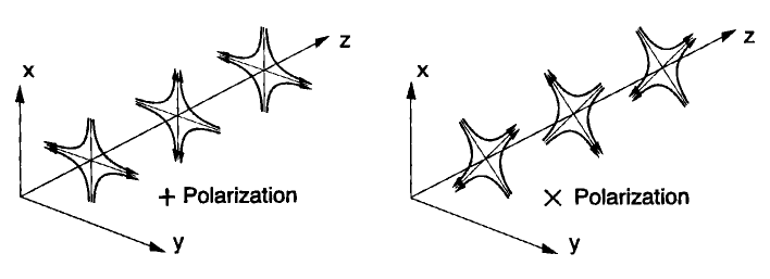
Figure 1: Lines of force for a purely $+$ GW (left), and for a purely $\times$ GW (right). Figure kindly provided by Kip Thorne; originally published in Ref. [44].

Of course, we don’t expect nature to provide GWs that so perfectly align with our detectors. In general, we will need to account for the detector’s antenna pattern, meaning that we will be sensitive to some weighted combination of the two polarizations, with the weights depending upon the location of a source on the sky, and the relative orientation of the source and the detector. See Ref. [45], Eqs. (104a,b) and associated text for further discussion.

Finally, in our analysis so far of detection we have assumed that the only contribution to the metric perturbation is the GW contribution. However, in reality time-varying near zone gravitational fields produced by sources in the vicinity of the detector will also be present. From Eq. (3.10) we see that the quantity that is actually measured by interferometric detectors is the space-time-space-time or electric-type piece $R_{itjt}$ of the Riemann tensor (or more precisely the time-varying piece of this within the frequency band of the detector). From the general expression (2.70) for this quantity we see that $R_{itjt}$ contains contributions from both $h_{ij}^{\rm TT}$ describing GWs, and also additional terms describing the time-varying near zone gravitational fields. There is no way for the detector to separate these two contributions, and the time-varying near zone gravitational fields produced by motions of bedrock, air, human bodies, and tumbleweeds can all contribute to the output of the detector and act as sources of noise [46, 47, 48].

4 The generation of gravitational waves: Putting in the source

4.1 Slow-motion sources in linearized gravity

Gravitational waves are generated by the matter source term on the right hand side of the linearized Einstein equation

$$\Box{\bar{h}}_{ab}=-16\pi T_{ab}\;,$$ (4.1)

cf. Eq. (2.15) (presented here in Lorentz gauge). In this section we will compute the leading order contribution to the spatial components of the metric perturbation for a source whose internal motions are slow compared to the speed of light (“slow-motion sources”). We will then compute the TT piece of the metric perturbation to obtain the standard quadrupole formula for the emitted radiation.

Equation (4.1) can be solved by using a Green’s function. A wave equation with source generically takes the form

$$\Box f(t,{\bf x})=s(t,{\bf x})\;,$$ (4.2)

where $f(t,{\bf x})$ is the radiative field, depending on time $t$ and position ${\bf x}$, and $s(t,{\bf x})$ is a source function. The Green’s function $G(t,{\bf x};t^{\prime},{\bf x}^{\prime})$ is the field which arises due to a delta function source; it tells how much field is generated at the “field point” $(t,{\bf x})$ per unit source at the “source point” $(t^{\prime},{\bf x}^{\prime})$:

$$\Box G(t,{\bf x};t^{\prime},{\bf x}^{\prime})=\delta(t-t^{\prime})\delta({\bf x}-{\bf x}^{\prime})\;.$$ (4.3)

The field which arises from our actual source is then given by integrating the Green’s function against $s(t,{\bf x})$:

$$f(t,{\bf x})=\int dt^{\prime}d^{3}x^{\prime}\,G(t,{\bf x};t^{\prime},{\bf x}^{\prime})\,s(t^{\prime},{\bf x}^{\prime})\;\;.$$ (4.4)

The Green’s function associated with the wave operator $\Box$ is very well known (see, e.g., [49]):

$$G(t,{\bf x};t^{\prime},{\bf x}^{\prime})=-\frac{\delta(t^{\prime}-[t-|{\bf x}-{\bf x}^{\prime}|/c])}{4\pi|{\bf x}-{\bf x}^{\prime}|}\;.$$ (4.5)

The quantity $t-|{\bf x}-{\bf x}^{\prime}|/c$ is the retarded time; it takes into account the lag associated with the propagation of information from events at ${\bf x}$ to position ${\bf x}^{\prime}$. The speed of light $c$ has been restored here to emphasize the causal nature of this Green’s function; we set it back to unity in what follows.

Applying this result to Eq. (4.1), we find

$${\bar{h}}_{ab}(t,{\bf x})=4\int d^{3}x^{\prime}\frac{T_{ab}(t-|{\bf x}-{\bf x}^{\prime}|,{\bf x}^{\prime})}{|{\bf x}-{\bf x}^{\prime}|}\;.$$ (4.6)

As already mentioned, the radiative degrees of freedom are contained entirely in the spatial part of the metric, projected transverse and traceless. First, consider the spatial part of the metric:

$${\bar{h}}_{ij}(t,{\bf x})=4\int d^{3}x^{\prime}\frac{T^{ij}(t-|{\bf x}-{\bf x}^{\prime}|,{\bf x}^{\prime})}{|{\bf x}-{\bf x}^{\prime}|}\;.$$ (4.7)

We have raised indices on the right-hand side, using the rule that the position of spatial indices in linearized theory is irrelevant.

We now evaluate this quantity at large distances from the source. This allows us to replace the factor $|{\bf x}-{\bf x}^{\prime}|$ in the denominator with $r=|{\bf x}|$. The corresponding fractional errors scale as $\sim L/r$, where $L$ is the size of the source; these errors can be neglected. We also make the same replacement in the time argument of $T_{ij}$:

$$T_{ij}(t-|{\bf x}-{\bf x}^{\prime}|,{\bf x}^{\prime})\approx T_{ij}(t-r,{\bf x}^{\prime}).$$ (4.8)

Using the formula $|{\bf x}-{\bf x}^{\prime}|=r-n^{i}x^{{}^{\prime}\,i}+O(1/r)$ where $n^{i}=x^{i}/r$, we see that the fractional errors generated by the replacement (4.8) scale as $L/\tau$, where $\tau$ is the timescale over which the system is changing. This quantity is just the velocity of internal motions of the source (in units with $c=1$), and is therefore small compared to one by our assumption. These replacements give

$${\bar{h}}_{ij}(t,{\bf x})=\frac{4}{r}\int d^{3}x^{\prime}\,T^{ij}(t-r,{\bf x}^{\prime})\;,$$ (4.9)

which is the first term in a multipolar expansion of the radiation field.

Equation (4.9) almost gives us the quadrupole formula that describes GW emission (at leading order). To get the rest of the way there, we need to massage this equation a bit. The stress-energy tensor must be conserved, which means $\partial_{a}T^{ab}=0$ in linearized theory. Breaking this up into time and space components, we have

$$\partial_{t}T^{tt}+\partial_{i}T^{ti} = 0\,,$$ (4.10)

$$\partial_{t}T^{ti}+\partial_{j}T^{ij} = 0\,.$$ (4.11)

From this, it follows rather simply that

$$\partial^{2}_{t}T^{tt}=\partial_{k}\partial_{l}T^{kl}\;.$$ (4.12)

Multiply both sides of this equation by $x^{i}x^{j}$. We first manipulate the left-hand side:

$$\partial^{2}_{t}T^{tt}x^{i}x^{j}=\partial_{t}^{2}\left(T^{tt}x^{i}x^{j}\right)\;.$$ (4.13)

Next, manipulate the right-hand side of Eq. (4.12), multiplied by $x^{i}x^{j}$:

$$\partial_{k}\partial_{l}T^{kl}x^{i}x^{j}=\partial_{k}\partial_{l}\left(T^{kl}x^{i}x^{j}\right)-2\partial_{k}\left(T^{ik}x^{j}+T^{kj}x^{i}\right)+2T^{ij}\;.$$ (4.14)

This identity is easily verified by expanding the derivatives and applying the identity $\partial_{i}x^{j}={\delta_{i}}^{j}$. We thus have

$$\partial_{t}^{2}\left(T^{tt}x^{i}x^{j}\right)=\partial_{k}\partial_{l}\left(T^{kl}x^{i}x^{j}\right)-2\partial_{k}\left(T^{ik}x^{j}+T^{kj}x^{i}\right)+2T^{ij}\;.$$ (4.15)

This yields

$$\frac{4}{r}\int d^{3}x^{\prime}\,T_{ij} = \frac{4}{r}\int d^{3}x^{\prime}\left[\frac{1}{2}\partial_{t}^{2}\left(T^{tt}x^{\prime i}x^{\prime j}\right)+\partial_{k}\left(T^{ik}x^{\prime j}+T^{kj}x^{\prime i}\right)\right.$$ (4.16)

$$\left.\qquad\qquad-\frac{1}{2}\partial_{k}\partial_{l}\left(T^{kl}x^{\prime i}x^{\prime j}\right)\right]$$

$$= \frac{2}{r}\int d^{3}x^{\prime}\,\partial_{t}^{2}\left(T^{tt}x^{\prime i}x^{\prime j}\right)$$

$$= \frac{2}{r}\frac{\partial^{2}}{\partial t^{2}}\int d^{3}x^{\prime}\,T^{tt}x^{\prime i}x^{\prime j}$$

$$= \frac{2}{r}\frac{\partial^{2}}{\partial t^{2}}\int d^{3}x^{\prime}\,\rho\,x^{\prime i}x^{\prime j}\;.$$

In going from the first line to the second, we used the fact that the second and third terms under the integral are divergences. Using Gauss’s theorem, they can thus be recast as surface integrals; taking the surface outside the source, their contribution is zero. In going from the second line to the third, we used the fact that the integration domain is not time dependent, so we can take the derivatives out of the integral. Finally, we used the fact that $T^{tt}$ is the mass density $\rho$. Defining the second moment $I_{ij}$ of the mass distribution via

$$I_{ij}(t)=\int d^{3}x^{\prime}\,\rho(t,{\bf x}^{\prime})\,x^{\prime i}x^{\prime j}\;,$$ (4.17)

and combining Eqs. (4.9) and (4.16) now gives

$${\bar{h}}_{ij}(t,{\bf x})=\frac{2}{r}\frac{d^{2}I_{ij}(t-r)}{dt^{2}}\;.$$ (4.18)

When we subtract the trace from $I_{ij}$, we obtain the quadrupole moment tensor:

$${\cal I}_{ij}=I_{ij}-\frac{1}{3}\delta_{ij}I,\qquad I=I_{ii}\;.$$ (4.19)

This tensor will prove handy shortly.

To complete the derivation, we must project out the non-TT pieces of the right-hand side of Eq. (4.18). Since we are working to leading order in $1/r$, at each field point ${\bf x}$ this operation reduces to algebraically projecting the tensor perpendicularly to the local direction of propagation ${\bf n}={\bf x}/r$, and subtracting off the trace. It is useful to introduce the projection tensor,

$$P_{ij}=\delta_{ij}-n_{i}n_{j}\;.$$ (4.20)

This tensor eliminates vector components parallel to ${\bf n}$, leaving only transverse components. Thus,

$${\bar{h}}^{T}_{ij}={\bar{h}}_{kl}P_{ik}P_{jl}$$ (4.21)

is a transverse tensor. Finally, we remove the trace; what remains is

$$h^{\rm TT}_{ij} = {\bar{h}}_{kl}P_{ik}P_{jl}-\frac{1}{2}P_{ij}P_{kl}{\bar{h}}_{kl}\;.$$ (4.22)

Substituting Eq. (4.18) into (4.22), we obtain our final quadrupole formula:

$$h^{\rm TT}_{ij}(t,{\bf x})=\frac{2}{r}\frac{d^{2}{\cal I}_{kl}(t-r)}{dt^{2}}\left[P_{ik}({\bf n})P_{jl}({\bf n})-\frac{1}{2}P_{kl}({\bf n})P_{ij}({\bf n})\right]\;.$$ (4.23)

4.2 Extension to sources with non-negligible self gravity

Our derivation of the quadrupole formula (4.23) assumed the validity of the linearized Einstein equations. In particular, the derivation is not applicable to systems with weak (Newtonian) gravity whose dynamics are dominated by self-gravity, such as binary star systems. This shortcoming of the above linearized-gravity derivation of the quadrupole formula was first pointed out by Eddington. However, it is very straightforward to extend the derivation to encompass systems with non-negligible self gravity.

In full general relativity we define the quantity ${\bar{h}}^{ab}$ via

$$\sqrt{-g}g^{ab}=\eta^{ab}-{\bar{h}}^{ab},$$ (4.24)

where $\eta^{ab}\equiv{\rm diag}(-1,1,1,1)$. When gravity is weak this definition coincides with our previous definition of ${\bar{h}}^{ab}$ as a trace-reversed metric perturbation. We impose the harmonic gauge condition

$$\partial_{a}(\sqrt{-g}g^{ab})=\partial_{a}{\bar{h}}^{ab}=0.$$ (4.25)

In this gauge the Einstein equation can be written

$$\Box_{\rm flat}{\bar{h}}^{ab}=-16\pi(T^{ab}+t^{ab})$$ (4.26)

where $\Box_{\rm flat}\equiv\eta^{ab}\partial_{a}\partial_{b}$ is the flat-spacetime wave operator, and $t^{ab}$ is a pseudotensor that is constructed from ${\bar{h}}^{ab}$. Taking a coordinate divergence of this equation and using the gauge condition (4.25) shows that stress-energy conservation can be written

$$\partial_{a}(T^{ab}+t^{ab})=0.$$ (4.27)

Equations (4.25), (4.26) and (4.27) are precisely the same equations as are used in the linearized-gravity derivation of the quadrupole formula, except for the fact that the stress energy tensor $T^{ab}$ is replaced by $T^{ab}+t^{ab}$. Therefore the derivation of the last subsection carries over, with the one modification that the formula (4.17) for $I_{ij}$ is replaced by

$$I_{ij}(t)=\int d^{3}x^{\prime}\left[T^{tt}(t,{\bf x}^{\prime})+t^{tt}(t,{\bf x}^{\prime})\right]x^{\prime i}x^{\prime j}.$$ (4.28)

In this equation the term $t^{tt}$ describes gravitational binding energy, roughly speaking. For systems with weak gravity, this term is negligible in comparison with the term $T^{tt}$ describing the rest-masses of the bodies. Therefore the quadrupole formula (4.23) and the original definition (4.17) of $I_{ij}$ continue to apply to the more general situation considered here.

4.3 Dimensional analysis

The rough form of the leading GW field that we just derived, Eq. (4.23), can be deduced using simple physical arguments. First, we define some moments of the mass distribution. The zeroth moment is just the mass itself:

$$M_{0}\equiv\int\rho\,d^{3}x=M\;.$$ (4.29)

(More accurately, this is the total mass-energy of the source.) Next, we define the dipole moment:

$$M_{1}\equiv\int\rho\,x_{i}\,d^{3}x=ML_{i}\;.$$ (4.30)

$L_{i}$ is a vector with the dimension of length; it describes the displacement of the center of mass from our chosen origin. (As such, $M_{1}$ is clearly not a very meaningful quantity — we can change its value simply by choosing a different origin.)

If our mass distribution exhibits internal motion, then moments of the mass current, $j_{i}=\rho v_{i}$, are also important. The first moment is the spin angular momentum:

$$S_{1}\equiv\int\rho v_{j}\,x_{k}\,\epsilon_{ijk}\,d^{3}x=S_{i}\;.$$ (4.31)

Finally, we look at the second moment of the mass distribution:

$$M_{2}\equiv\int\rho\,x_{i}\,x_{j}\,d^{3}x=ML_{ij}$$ (4.32)

where $L_{ij}$ is a tensor with the dimension length squared.

Using dimensional analysis and simple physical arguments, it is simple to see that the first moment that can contribute to GW emission is $M_{2}$. Consider first $M_{0}$. We want to combine $M_{0}$ with the distance to our source, $r$, in such a way as to produce a dimensionless wavestrain $h$. The only way to do this (bearing in mind that the strain should fall off as $1/r$, and restoring factors of $G$ and $c$) is to put

$$h\sim\frac{G}{c^{2}}\frac{M_{0}}{r}\;.$$ (4.33)

Does this formula make sense for radiation? Not at all! Conservation of mass-energy tells us that $M_{0}$ for an isolated source cannot vary dynamically. This $h$ cannot be radiative; it corresponds to a Newtonian potential, rather than a GW.

How about the moment $M_{1}$? In order to get the dimensions right, we must take one time derivative:

$$h\sim\frac{G}{c^{3}}\frac{d}{dt}\frac{M_{1}}{r}\;.$$ (4.34)

(The extra factor of $c$ converts the dimension of the time derivative to space, so that the whole expression is dimensionless.) Think carefully about the derivative of $M_{1}$:

$$\frac{dM_{1}}{dt}=\frac{d}{dt}\int\rho\,x_{i}\,d^{3}x=\int\rho\,v_{i}\,d^{3}x=P_{i}\;.$$ (4.35)

This is the total momentum of our source. Our guess for the form of a wave corresponding to $M_{1}$ becomes

$$h\sim\frac{G}{c^{3}}\frac{P}{r}\;.$$ (4.36)

Can this describe a GW? Again, not a chance: The momentum of an isolated source must be conserved. By boosting into a different Lorentz frame, we can always set $P=0$. Terms like this can only be gauge artifacts; they do not correspond to radiation. [Indeed, terms like (4.36) appear in the metric of a moving black hole, and correspond to the relative velocity of the hole and the observer; see [50], Chapter 5.]

How about $S_{1}$? Dimensional analysis tells us that radiation from $S_{1}$ must take the form

$$h\sim\frac{G}{c^{4}}\frac{d}{dt}\frac{S_{1}}{r}.$$ (4.37)

Conservation of angular momentum tells us that the total spin of an isolated system cannot change, so we reject this term for the same reason that we rejected (4.33) — it cannot correspond to radiation.

Finally, we examine $M_{2}$:

$$h\sim\frac{G}{c^{4}}\frac{d^{2}}{dt^{2}}\frac{M_{2}}{r}\;.$$ (4.38)

There is no conservation principle that allows us to reject this term. Comparing to Eq. (4.23), we see that this is the quadrupole formula we derived earlier, up to numerical factors.

In “normal” units, the prefactor of this formula turns out to be $G/c^{4}$ — a small number divided by a very big number. In order to generate interesting amounts of GWs, the quadrupole moment’s variation must be enormous. The only interesting sources of GWs will be those which have very large masses undergoing extremely rapid variation; even in this case the strain we expect from typical sources is tiny. The smallness of GWs reflects the fact that gravity is the weakest of the fundamental interactions.

4.4 Numerical estimates

Consider a binary star system, with stars of mass $m_{1}$ and $m_{2}$ in a circular orbit with separation $R$. The quadrupole moment is given by

$${\cal I}_{ij}=\mu\left(x_{i}x_{j}-\frac{1}{3}R^{2}\delta_{ij}\right)\;,$$ (4.39)

where $\mu=m_{1}m_{2}/(m_{1}+m_{2})$ is the binary’s reduced mass and ${\bf x}$ is the relative displacement, with $|{\bf x}|=R$. We use the center-of-mass reference frame, and choose the coordinate axes so that the binary lies in the $xy$ plane, so $x=x_{1}=R\cos\Omega t$, $y=x_{2}=R\sin\Omega t$, $z=x_{3}=0$. Let us further choose to evaluate the field on the $z$ axis, so that ${\bf n}$ points in the $z$-direction. The projection operators in Eq. (4.23) then simply serve to remove the $zj$ components of the tensor. Bearing this in mind, the quadrupole formula (4.23) yields

$$h^{\rm TT}_{ij}=\frac{2\ddot{\cal I}_{ij}}{r}\;.$$ (4.40)

The quadrupole moment tensor is

$${\cal I}_{ij}=\mu R^{2}\left[\matrix{\cos^{2}\Omega t-\frac{1}{3}&\cos\Omega t\sin\Omega t&0\cr\cos\Omega t\sin\Omega t&\cos^{2}\Omega t-\frac{1}{3}&0\cr 0&0&-\frac{1}{3}\cr}\right]\;;$$ (4.41)

its second derivative is

$$\ddot{\cal I}_{ij}=-2\Omega^{2}\mu R^{2}\left[\matrix{\cos 2\Omega t&\sin 2\Omega t&0\cr-\sin 2\Omega t&-\cos 2\Omega t&0\cr 0&0&0\cr}\right]\;.$$ (4.42)

The magnitude $h$ of a typical non-zero component of $h^{\rm TT}_{ij}$ is

$$h=\frac{4\mu\Omega^{2}R^{2}}{r}=\frac{4\mu M^{2/3}\Omega^{2/3}}{r}\;.$$ (4.43)

We used Kepler’s 3rd law to replace $R$ with powers of the orbital frequency $\Omega$ and the total mass $M=m_{1}+m_{2}$. For the purpose of our numerical estimate, we will take the members of the binary to have equal masses, so that $\mu=M/4$:

$$h=\frac{M^{5/3}\Omega^{2/3}}{r}\;.$$ (4.44)

Finally, we insert numbers corresponding to plausible sources:

$$h \simeq 10^{-21}\left(\frac{M}{2\,M_{\odot}}\right)^{5/3}\left(\frac{1\,\mbox{hour}}{P}\right)^{2/3}\left(\frac{1\,\mbox{kiloparsec}}{r}\right)$$ (4.45)

$$\simeq 10^{-22}\left(\frac{M}{2.8\,M_{\odot}}\right)^{5/3}\left(\frac{0.01\,\mbox{sec}}{P}\right)^{2/3}\left(\frac{100\,\mbox{Megaparsecs}}{r}\right)\;.$$

The first line corresponds roughly to the mass, distance and orbital period ($P=2\pi/\Omega$) expected for the many close binary white dwarf systems in our galaxy. Such binaries are so common that they are likely to be a confusion limited source of GWs for space-based detectors, acting in some cases as an effective source of noise. The second line contains typical parameter values for binary neutron stars that are on the verge of spiralling together and merging. Such waves are targets for the ground-based detectors that have recently begun operations. The tiny magnitude of these waves illustrates why detecting GWs is so difficult.

5 Linearized theory of gravitational waves in a curved background

At the most fundamental level, GWs can only be defined within the context of an approximation in which the wavelength of the waves is much smaller than lengthscales characterizing the background spacetime in which the waves propagate. In this section, we discuss perturbation theory of curved spacetimes, describe the approximation in which GWs can be defined, and derive the effective stress tensor which describes the energy content of GWs. The material in this section draws on the treatments given in Chapter 35 of Misner, Thorne and Wheeler [4], Sec. 7.5 of Wald [51], and the review articles [31, 32].

5.1 Perturbation theory of curved vacuum spacetimes

Throughout this section we will for simplicity restrict attention to vacuum spacetime regions. We consider a one-parameter family of solutions of the vacuum Einstein equation, parameterized by $\varepsilon$, of the form

$$g_{ab}=g_{ab}^{\rm B}+\varepsilon h_{ab}+\varepsilon^{2}j_{ab}+O(\varepsilon^{3})\;.$$ (5.1)

Here $g_{ab}^{\rm B}$ is the background metric; it was taken to be the Minkowski metric in Secs. 2, 4 and 2.2. Here we allow $g_{ab}^{\rm B}$ to be any vacuum solution of the Einstein equations. The quantity $h_{ab}$ is the linear order metric perturbation, as in the previous sections; $j_{ab}$ is a second order metric perturbation which will be used in Sec. 5.3. We can regard $\varepsilon$ as a formal expansion parameter; we set its value to unity at the end of our calculations.

The derivation of the linearized Einstein equation proceeds as before. Most of the formulae for linearized perturbations of Minkowski spacetime continue to apply, with $\eta_{ab}$ replaced by $g^{\rm B}_{ab}$, and with partial derivatives $\partial_{a}$ replaced by covariant derivatives with respect to the background, $\nabla^{\rm B}_{a}$. Some of the formulae acquire extra terms involving coupling to the background Riemann tensor.

Inserting Eq. (5.1) into the formula for connection coefficients gives

$$\Gamma^{a}_{bc} = \frac{1}{2}g^{ad}\left(\partial_{c}g_{db}+\partial_{b}g_{dc}-\partial_{d}g_{bc}\right)$$

$$= \frac{1}{2}\left(g^{{\rm B}\,ad}-\varepsilon h^{ad}\right)\left(\partial_{c}g^{\rm B}_{db}+\varepsilon\partial_{c}h_{db}+\partial_{b}g^{\rm B}_{dc}\right.$$

$$\qquad\qquad\qquad\left.+\varepsilon\partial_{b}h_{dc}-\partial_{d}g^{\rm B}_{bc}-\varepsilon\partial_{d}h_{bc}\right)+O(\varepsilon^{2})$$

$$= \Gamma^{{\rm B}\,a}_{\ \ bc}+\varepsilon\delta\Gamma^{a}_{bc}+O(\varepsilon^{2})\;.$$ (5.3)

Here $\Gamma^{{\rm B}\,a}_{\ \ bc}$ are the connection coefficients of the background metric $g_{ab}^{\rm B}$, and the first order corrections to the connection coefficients are given by

$$\delta\Gamma^{a}_{bc} = -\frac{1}{2}h^{ad}g^{\rm B}_{de}\Gamma^{{\rm B}\,e}_{\ \ bc}+\frac{1}{2}g^{{\rm B}\,ad}\left(\partial_{c}h_{db}+\partial_{b}h_{dc}-\partial_{d}h_{bc}\right)$$ (5.4)

$$= \frac{1}{2}g^{{\rm B}\,ad}\left(\nabla^{\rm B}_{c}h_{db}+\nabla^{\rm B}_{b}h_{dc}-\nabla^{\rm B}_{d}h_{bc}\right)\;,$$

where $\nabla^{\rm B}_{a}$ is the covariant derivative operator associated with the background metric. Equation (5.4) can be derived more easily, at any given point in spacetime, by evaluating the expression (5.1) in a coordinate system in which the background connection coefficients vanish at that point, so that $\partial_{a}=\nabla_{a}^{\rm B}$. The result (5.4) for general coordinate systems then follows from general covariance.

Next, insert the expansion (5.3) of the connection coefficients into the formula

$$R^{a}_{\ bcd}=\partial_{c}\Gamma^{a}_{bd}-\partial_{d}\Gamma^{a}_{bc}+\Gamma^{a}_{ce}\Gamma^{e}_{bd}-\Gamma^{a}_{de}\Gamma^{e}_{bc}$$ (5.5)

for the Riemann tensor. Evaluating the result in a coordinate system in which $\Gamma^{{\rm B}\,a}_{\ \ bc}=0$ at the point of evaluation gives

$$R^{a}_{\ bcd} = \partial_{c}\Gamma^{{\rm B}\,a}_{\ \ bd}-\partial_{d}\Gamma^{{\rm B}\,a}_{\ \ bc}+\varepsilon\left(\partial_{c}\delta\Gamma^{a}_{bd}-\partial_{d}\delta\Gamma^{a}_{bc}\right)+O(\varepsilon^{2})$$ (5.6)

$$= R^{{\rm B}\,a}_{\ \ \ bcd}+\varepsilon\delta R^{a}_{\ bcd}+O(\varepsilon^{2})\;.$$

Here $R^{{\rm B}\,a}_{\ \ \ bcd}$ is the Riemann tensor of the background metric, and $\delta R^{a}_{\ bcd}=\partial_{c}\delta\Gamma^{a}_{bd}-\partial_{d}\delta\Gamma^{a}_{bc}$ is the linear perturbation to the Riemann tensor. It follows from general covariance that the expression for $\delta R^{a}_{\ bcd}$ in a general coordinate system is

$$\delta R^{a}_{\ bcd}=\nabla^{{\rm B}}_{c}\delta\Gamma^{a}_{bd}-\nabla^{{\rm B}}_{d}\delta\Gamma^{a}_{bc}\;.$$ (5.7)

Using the expression (5.4) now gives

$$\delta R^{a}_{\ bcd} = \frac{1}{2}\bigg{(}\nabla^{{\rm B}}_{c}\nabla^{{\rm B}}_{b}h^{a}_{\ d}+\nabla^{{\rm B}}_{c}\nabla^{{\rm B}}_{d}h^{a}_{\ b}-\nabla^{{\rm B}}_{c}\nabla^{{\rm B}\,a}h_{bd}$$ (5.8)

$$-\nabla^{{\rm B}}_{d}\nabla^{{\rm B}}_{b}h^{a}_{\ c}-\nabla^{{\rm B}}_{d}\nabla^{{\rm B}}_{c}h^{a}_{\ b}+\nabla^{{\rm B}}_{d}\nabla^{{\rm B}\,a}h_{bc}\bigg{)}\;.$$

Contracting on the indices $a$ and $c$ yields the linearized Ricci tensor $\delta R_{bd}$:

$$\delta R_{bd}=-\frac{1}{2}\Box^{\rm B}h_{bd}-\frac{1}{2}\nabla^{{\rm B}}_{d}\nabla^{{\rm B}}_{b}h+\nabla^{{\rm B}}_{a}\nabla^{{\rm B}}_{(b}h^{a}_{\ d)}\;.$$ (5.9)

where $\Box^{\rm B}\equiv\nabla^{{\rm B}}_{a}\nabla^{{\rm B}\,a}$, indices are raised and lowered with the background metric, and $h=h^{a}_{\ a}$. Reversing the trace to obtain the linearized Einstein tensor $\delta G_{bd}$, and writing the result in terms of the trace-reversed metric perturbation

$${\bar{h}}_{ab}=h_{ab}-\frac{1}{2}g^{\rm B}_{ab}g^{{\rm B}\,cd}h_{cd}$$ (5.10)

yields the linearized vacuum Einstein equation

$$0=\delta G_{bd} = -\frac{1}{2}\Box^{\rm B}{\bar{h}}_{bd}+R^{\rm B}_{adbc}{\bar{h}}^{ac}$$ (5.11)

$$-\frac{1}{2}g^{\rm B}_{bd}\nabla^{\rm B}_{a}\nabla^{\rm B}_{c}{\bar{h}}^{ac}+\frac{1}{2}\nabla^{\rm B}_{b}\nabla^{\rm B}_{a}{\bar{h}}^{a}_{\ d}+\frac{1}{2}\nabla^{\rm B}_{d}\nabla^{\rm B}_{a}{\bar{h}}^{a}_{\ b}\;.$$

As in Sec. 2, the linearized Einstein equation can be simplified considerably by a suitable choice of gauge. Under a gauge transformation parameterized by the vector field $\xi^{a}$, the metric transforms as

$$h_{ab}\to h^{\prime}_{ab}=h_{ab}-2\nabla^{\rm B}_{(a}\xi_{b)}\;;$$ (5.12)

the divergence of the trace-reversed metric perturbation thus transforms as

$$\nabla^{{\rm B}\,a}{\bar{h}}^{\prime}_{ab}=\nabla^{{\rm B}\,a}{\bar{h}}_{ab}-\Box^{\rm B}\xi_{b}\;.$$ (5.13)

We can enforce in the new gauge the transverse condition

$$\nabla^{{\rm B}\,a}{\bar{h}}^{\prime}_{ab}=0$$ (5.14)

by requiring that $\xi_{b}$ satisfy the wave equation $\Box^{\rm B}\xi_{b}=\nabla^{{\rm B}\,a}{\bar{h}}_{ab}$. We can further specialize the gauge to satisfy $h^{\prime}=0$. Dropping the primes, the metric perturbation is thus traceless and transverse:

$$\nabla^{{\rm B}\,a}h_{ab}=h=0.$$ (5.15)

In this gauge the linearized Einstein equation (5.11) simplifies to

$$0=\delta G_{bd}=-\frac{1}{2}\Box^{\rm B}h_{bd}+R^{\rm B}_{adbc}h^{ac}\;.$$ (5.16)

(Note, however, that one cannot in this context impose the additional gauge conditions $h_{0a}=0$ used in the definition of TT gauge for perturbations of flat spacetime.)

To see that the traceless condition $h=0$ can be achieved, note that the trace transforms as

$$h\to h^{\prime}=h-2\nabla^{{\rm B}\,a}\xi_{a}\;.$$ (5.17)

Therefore it is sufficient to find a vector field $\xi^{a}$ that satisfies $\Box^{\rm B}\xi_{a}=0$ and

$$\nabla^{B\,a}\xi_{a}-h/2=0.$$ (5.18)

We can choose initial data for $\xi_{a}$ on any Cauchy hypersurface for which the quantity (5.18) and also its normal derivative vanish. Since the quantity (5.18) satisfies the homogeneous wave equation by Eqs. (5.11) and (5.14), it will vanish everywhere.

The wave equation (5.16) differs from its flat spacetime counterpart (2.16) in two respects: First, there is an explicit coupling to the background Riemann tensor; and second, there is a coupling to the background curvature through the connection coefficients that appear in the covariant wave operator $\Box^{\rm B}$. In the limit (discussed below) where the wavelength of the waves is much smaller than the lengthscales characterizing the background metric, these couplings have the effect of causing gradual evolution in the properties of the wave. These gradual changes can be described using the formalism of geometric optics, which shows that GWs travel along null geodesics with slowly evolving amplitudes and polarizations. See Ref. [31] for a detailed description of this formalism. Outside of the geometric optics limit the curvature couplings in Eq. (5.16) can cause the dynamics of the metric perturbation to be strongly coupled to the dynamics of the background spacetime. An example of such coupling is the parametric amplification of metric perturbations during inflation in the early Universe [52].

5.2 General definition of gravitational waves: The geometric optics regime

The linear perturbation formalism described in the last section can be applied to any perturbations of any vacuum background spacetime. Its starting point is the separation of the spacetime metric into a background piece plus a perturbation. In most circumstances this separation is merely a mathematical device and can be chosen arbitrarily; no unique separation is determined by local physical measurements. [Although $g_{ab}^{\rm B}$ and $h_{ab}$ are uniquely determined once one specifies the one parameter family of metrics $g_{ab}(\varepsilon)$, a given physical situation will be described by a single metric $g_{ab}(\varepsilon_{0})$ for some fixed value of $\varepsilon_{0}$ of $\varepsilon$, not by the one parameter family of metrics.] However, in special circumstances, a unique separation into background plus perturbation is determined by local physical measurements, and it is only in this context that GWs can be defined. Such circumstances arise when the wavelength $\lambda$ of the waves is very much smaller than the characteristic lengthscales ${\cal L}$ characterizing the background curvature. In this case one can define the background metric and perturbation, to linear order, via

$$g_{ab}^{\rm B} \equiv \langle g_{ab}\rangle\;,$$ (5.19)

$$\varepsilon h_{ab} \equiv g_{ab}-g_{ab}^{\rm B}\;.$$ (5.20)

Here the angular brackets $\langle...\rangle$ denote an average over lengthscales large compared to $\lambda$ but small compared to ${\cal L}$; a suitable covariant definition of such averaging has been given by Brill and Hartle [53]. A useful analogy to consider is the surface of an orange, which contains curvatures on two different lengthscales: An overall, roughly spherical background curvature (analogous to the background metric), and a dimpled texture on small scales (analogous to the GW). The regime $\lambda\ll{\cal L}$ is called the geometric optics regime.

We will argue below that the short-wavelength perturbation $\varepsilon h_{ab}$ gives rise to an effective stress tensor of order $\varepsilon^{2}h^{2}/\lambda^{2}$, where $h$ is a typical size of $h_{ab}$. This effective stress tensor contributes to the curvature of the background metric $g_{ab}^{\rm B}$. This contribution to the curvature is $\;\hbox to0.0pt{\lower 2.5pt\hbox{$\sim$}\hss}\raise 1.5pt\hbox{$<$}\;1/{\cal L}^{2}$. It follows that $\varepsilon^{2}h^{2}/\lambda^{2}\;\hbox to0.0pt{\lower 2.5pt\hbox{$\sim$}\hss}\raise 1.5pt\hbox{$<$}\;1/{\cal L}^{2}$, or

$$\varepsilon h\;\hbox to0.0pt{\lower 2.5pt\hbox{$\sim$}\hss}\raise 1.5pt\hbox{$<$}\;{\lambda\over{\cal L}}\;.$$ (5.21)

Since we are assuming that $\lambda\ll{\cal L}$, it follows that the short-wavelength piece $\varepsilon h_{ab}$ of the metric is small compared to the background metric, and so we can use the perturbation formalism of Sec. 5.1. Consider now the splitting of the Riemann tensor into a background piece plus a perturbation given by Eq. (5.6):

$$R_{abcd}=R^{{\rm B}}_{abcd}+\varepsilon\delta R_{abcd}+O(\varepsilon^{2})\;.$$ (5.22)

By the definition (5.19) of the background metric, it follows that $g_{ab}^{\rm B}$ and $R^{{\rm B}}_{abcd}$ vary only over lengthscales $\;\hbox to0.0pt{\lower 2.5pt\hbox{$\sim$}\hss}\raise 1.5pt\hbox{$>$}\;{\cal L}$, and therefore it follows that to a good approximation

$$\langle R^{\rm B}_{abcd}\rangle=R^{\rm B}_{abcd}\;.$$ (5.23)

Hence the perturbation to the Riemann tensor can be obtained via

$$\varepsilon\delta R_{abcd}=R_{abcd}-\langle R_{abcd}\rangle\;,$$ (5.24)

the same unique and local procedure as for the metric perturbation (5.20). This Riemann tensor perturbation is often called the GW Riemann tensor; it is a tensor characterizing the GWs that propagates in the background metric $g_{ab}^{\rm B}$.

The operational meaning of the GW fields $\varepsilon h_{ab}$ and $\varepsilon\delta R_{abcd}$ follows directly from the equivalence principle and from their meaning in the context of flat spacetime (Sec. 2). Specifically, suppose that ${\cal P}$ is a point in spacetime, and pick a coordinate system in which $g_{ab}^{\rm B}=\eta_{ab}$ and $\Gamma^{{\rm B}\,a}_{\ \ bc}=0$ at ${\cal P}$. Then we have

$$g_{ab}=\eta_{ab}+O\left({x^{2}\over{\cal L}^{2}}\right)+\varepsilon h_{ab}+O(\varepsilon^{2})\;,$$ (5.25)

where $x$ is the distance from ${\cal P}$. Therefore, within a spacetime region around ${\cal P}$ in which $x\ll{\cal L}$, the flat-spacetime perturbation theory and measurement analysis of Sec. 2 can be applied. Thus, the gravitational waveforms seen by observers performing local experiments will just be given by components of the GW Riemann tensor in the observer’s local proper reference frames.

We remark that the splitting of the metric into a background plus a linear perturbation can sometimes be uniquely defined even in the regime $\lambda\sim{\cal L}$. Some examples are when the background spacetime is static (eg perturbations of a static star), or homogeneous (eg Friedman-Robertson-Walker cosmological models). In these cases the dynamic metric perturbation are not actually GWs, although their evolution can be computed using the linearized Einstein equation. For example, consider the evolution of a metric perturbation mode which is parametrically amplified during inflation in the early Universe. At early times during inflation, the mode’s wavelength $\lambda$ is smaller than the Hubble scale (${\cal L}$); the mode is said to be “inside the horizon”. Any excitation of the mode is locally measurable (although such modes are usually assumed to start in their vacuum state). As inflation proceeds, the mode’s wavelength redshifts and becomes larger due to the the rapid expansion of the Universe, and eventually becomes larger than the Hubble scale ${\cal L}$; the mode is then “outside the horizon”. At this point, excitations in the mode are not locally measurable and are thus not GWs. Finally, after inflation ends the mode “re-enters the horizon” and excitations of the mode are locally measurable. The mode is now a true GW once again.

Finally, we note that for perturbations of flat spacetime, the definition of GWs given here does not always coincide with the definition in terms of the TT component of the metric given in Sec. 2.2. However, far from sources of GWs (the regime relevant to observations), the two definitions do coincide. This is because the TT piece of the metric will vary on scales of a wavelength $\lambda$ which is short compared to the lengthscale $\sim r$ over which other pieces of the metric vary (except for other dynamic pieces of the metric such as the time-varying quadrupole term in the gauge-invariant field $\Phi$; those pieces vary on short lengthscales but are unimportant since they are smaller than the TT piece by a factor $\sim\lambda^{2}/r^{2}$ or smaller).

5.3 Effective stress-energy tensor of gravitational waves

Two major conceptual building blocks are needed for the derivation of the energy and momentum carried by GWs [54]: The perturbation theory of Sec. 5.1, generalized to second order in $\varepsilon$, and the separation of lengthscales $\lambda\ll{\cal L}$ discussed in the previous subsection.

We start by discussing the second order perturbation theory. By inserting the expansion (5.1) into the vacuum Einstein equation we obtain

$$0 = G_{ab}$$ (5.26)

$$= G_{ab}[g_{cd}^{\rm B}]+\varepsilon G_{ab}^{(1)}[h_{cd};g_{ef}^{\rm B}]+\varepsilon^{2}G_{ab}^{(1)}[j_{cd};g_{ef}^{\rm B}]+\varepsilon^{2}G_{ab}^{(2)}[h_{cd};g_{ef}^{\rm B}]$$

$$+O(\varepsilon^{3})\;.$$

Here $G_{ab}[g_{cd}^{\rm B}]$ is the Einstein tensor of the background metric, and $G_{ab}^{(1)}[...;g_{ef}^{\rm B}]$ is the linear differential operator on metric perturbations giving the linear perturbation to the Einstein tensor generated by a metric perturbation. The explicit expression for $G_{ab}^{(1)}[h_{cd},g_{ef}^{\rm B}]$ is given by Eq. (5.11). The term $G_{ab}^{(2)}[h_{cd};g_{ef}^{\rm B}]$ is the piece of the Einstein tensor that is quadratic in $h_{ab}$; it can be computed by extending the computation of Sec. (5.1) to one higher order, and is a sum of terms of the form $h_{ab}\nabla^{\rm B}_{c}\nabla^{\rm B}_{d}h_{ef}$ and $(\nabla_{a}^{\rm B}h_{bc})(\nabla^{\rm B}_{d}h_{ef})$ with various index contractions; see Eq. (35.58b) of MTW [4]. It’s worth recalling that $j_{ab}$ is a second order metric perturbation. We must take the calculation to second order to compute the effective stress energy tensor of the waves since an averaging is involved — the first order contribution vanishes by the oscillatory nature of the waves.

Equating to zero the coefficients of the different powers of $\varepsilon$ we obtain the vacuum Einstein equation for the background spacetime

$$G_{ab}[g^{\rm B}_{cd}]=0,$$ (5.27)

the linearized Einstein equation

$$G_{ab}^{(1)}[h_{cd};g_{ef}^{\rm B}]=0\;,$$ (5.28)

together with the equation for the second-order metric perturbation $j_{ab}$

$$G_{ab}^{(1)}[j_{cd};g_{ef}^{\rm B}]=-G_{ab}^{(2)}[h_{cd};g_{ef}^{\rm B}]\;.$$ (5.29)

We now specialize to the geometric optics regime $\lambda\ll{\cal L}$. We split the second order metric perturbation into a piece $\langle j_{ab}\rangle$ that is slowly varying, and a piece

$$\Delta j_{ab}=j_{ab}-\langle j_{ab}\rangle$$ (5.30)

that is rapidly varying. The full metric can be now be written

$$g_{ab}=\left(g_{ab}^{\rm B}+\varepsilon^{2}\langle j_{ab}\rangle\right)+\left(\varepsilon h_{ab}+\varepsilon^{2}\Delta j_{ab}\right)+O(\varepsilon^{3})\;,$$ (5.31)

where the first term varies slowly on lengthscales $\sim{\cal L}$, and the second term varies rapidly on lengthscales $\sim\lambda$. Consider next the average of the second-order Einstein equation (5.29). Using the fact that the averaging operation $\langle\ldots\rangle$ commutes with derivatives we get

$$G_{ab}^{(1)}[\langle j_{cd}\rangle;g_{ef}^{\rm B}]=-\langle G_{ab}^{(2)}[h_{cd};g_{ef}^{\rm B}]\rangle\;.$$ (5.32)

Subtracting Eq. (5.32) from Eq. (5.29) gives an equation for $\Delta j_{ab}$:

$$G^{(1)}_{ab}[\Delta j_{cd}]=-G_{ab}^{(2)}[h_{cd};g_{ef}^{\rm B}]+\langle G_{ab}^{(2)}[h_{cd};g_{ef}^{\rm B}]\rangle\;.$$ (5.33)

Equation (5.32) can be rewritten using Eq. (5.27) as

$$G_{ab}[g_{cd}^{\rm B}+\varepsilon^{2}\langle j_{cd}\rangle]=8\pi T_{ab}^{\rm GW,eff}+O(\varepsilon^{3})\;,$$ (5.34)

where the effective GW stress-energy tensor is

$$T_{ab}^{\rm GW,eff}=-{1\over 8\pi}\langle G_{ab}^{(2)}[h_{cd};g_{ef}^{\rm B}]\rangle\;.$$ (5.35)

In the effective Einstein equation (5.34), all the quantities vary slowly, on lengthscales $\sim{\cal L}$. The left-hand-side is the Einstein tensor of the slowly varying piece of the metric. The right hand side is the effective stress energy tensor, obtained by taking an average of the quadratic piece of the second order Einstein tensor. It follows from Eq. (5.34) that $T_{ab}^{\rm GW,eff}$ is conserved with respect to the metric $g_{ab}^{\rm B}+\varepsilon^{2}\langle j_{ab}\rangle$. In particular, to leading order in $\varepsilon$ it is conserved with respect to the background metric $g_{ab}^{\rm B}$.

The effect of the GWs is thus to give rise to a correction $\langle j_{ab}\rangle$ to the background metric. This correction is locally of the same order as $\Delta j_{ab}$, the rapidly varying piece of the second order metric perturbation. However, any measurements that probe only the long-lengthscale structure of the metric (for example measurements of the gravitating mass of a radiating source over timescales long compared to $\lambda$) are sensitive only to $\langle j_{ab}\rangle$. Thus, when one restricts attention to long lengthscales, GWs can thus be treated as any other form of matter source in general relativity. Typically $\langle j_{ab}\rangle$ grows secularly with time, while $\Delta j_{ab}$ does not.

A fairly simple expression for the effective stress-energy tensor can be obtained as follows. Schematically, the effective stress-energy tensor has the form

$$T_{ab}^{\rm GW,eff}\sim\&\langle h_{ab}\nabla^{\rm B}_{c}\nabla^{\rm B}_{d}h_{ef}\rangle+\&\langle(\nabla_{a}^{\rm B}h_{bc})(\nabla^{\rm B}_{d}h_{ef})\rangle\;,$$ (5.36)

where $\&$ means “a sum of terms obtained by taking various contractions of”. In this expression gradients scale as $1/\lambda$, so $\nabla_{c}^{\rm B}\nabla_{d}^{\rm B}\sim 1/\lambda^{2}$. However the commutator of two derivatives scales as the background Riemann tensor, which is of order $1/{\cal L}^{2}$. Therefore, up to corrections of order $\lambda^{2}/{\cal L}^{2}$ which can be neglected, one can freely commute covariant derivatives in the expression (5.36). Also, the average of any total derivative will vanish in the limit $\lambda\ll{\cal L}$ if the averaging lengthscale is taken to be $\sqrt{\lambda{\cal L}}$. Therefore one can flip derivatives from one factor to another inside the averages in Eq. (5.36), as in integration by parts. Using these manipulations the expression for the effective stress-energy tensor simplifies to [4, 54]

$$T_{ab}^{\rm GW,eff}=\frac{1}{32\pi}\left<\nabla^{\rm B}_{a}{\bar{h}}_{cd}\nabla_{b}^{\rm B}{\bar{h}}^{cd}-\frac{1}{2}\nabla^{\rm B}_{a}{\bar{h}}\nabla^{\rm B}_{b}{\bar{h}}-\nabla^{\rm B}_{a}{\bar{h}}_{bc}\nabla_{d}^{\rm B}{\bar{h}}^{cd}-\nabla^{\rm B}_{b}{\bar{h}}_{ac}\nabla_{d}^{\rm B}{\bar{h}}^{cd}\right>\;.$$ (5.37)

In gauges satisfying the transverse-traceless conditions (5.15) this reduces to

$$T_{ab}^{\rm GW,eff} = \frac{1}{32\pi}\left<\nabla^{\rm B}_{a}h_{cd}\nabla_{b}^{\rm B}h^{cd}\right>.$$ (5.38)

For example, for the plane wave propagating in the $z$ direction in flat spacetime, given by

$$h_{xx} = -h_{yy}=h_{0}\cos(\omega t-\omega z)\;,$$

$$h_{ab} = 0\quad\mbox{(all other components)}\;,$$ (5.39)

the energy density and energy flux are given by

$$T^{tt}=T^{tz}={h_{0}^{2}\omega^{2}\over 16\pi}\langle\cos^{2}(\omega t-\omega z)\rangle={h_{0}^{2}\omega^{2}\over 32\pi}.$$ (5.40)

If we restore factors of $G$ and $c$, and insert numbers typical of bursts of waves that we hope to detect, we get the energy flux

$$T^{tz}=1.5\,\,{\rm mW}\,\,{\rm m}^{-2}\left(\frac{h_{0}}{10^{-22}}\right)^{2}\,\left(\frac{f}{1\,{\rm kHz}}\right)^{2}\;$$ (5.41)

where $f=\omega/(2\pi)$. Note that this is a large energy flux by astronomical standards, despite the tiny value of $h_{0}$; it is comparable to the flux of reflected sunlight from a full moon [32].

6 A brief survey of gravitational wave astronomy

Having now reviewed the basic theory and properties of GWs, we conclude this article by very briefly surveying the properties of important potential sources of GWs. Our goal is to give some indication of the value that GWs may provide for astronomical observations; much of this material is updated from a previous survey article, Ref. [29]. We note that since the focus of this article is intended to be the theory GW sources (and that this article is significantly longer than was intended or requested), we are quite a bit more schematic in our treatment here than we have been in the rest of this paper. This final section is intended to be a very brief, somewhat superficial survey, rather than a detailed review.

We begin by contrasting gravitational radiation with electromagnetic radiation, which forms the basis for almost all current astronomical observations:

Electromagnetic waves interact strongly with matter; GWs do not. The weak interaction of GWs is both blessing and curse: It means that they propagate from emission to Earth-bound observers with essentially zero absorption, making it possible to probe astrophysics that is hidden or dark to electromagnetic observations — e.g., the coalescence and merger of black holes, the collapse of a stellar core, the dynamics of the early Universe. It also means that detecting GWs is very difficult. Also, because many of the best sources are hidden or dark, they are very poorly understood today — we know very little about what are likely to be some of the most important sources of GWs.

Electromagnetic radiation typically has a wavelength smaller than the size of the emitting system, and so can be used to form an image of the source. This is because electromagnetic radiation is usually generated by moving charges in the environment of some larger source — e.g., an atomic transition in interstellar gas, or emission from hot plasma in a stellar environment. By contrast, the wavelength of gravitational radiation is typically comparable to or larger than the size of the radiating source. GWs are generated by the bulk dynamics of the source itself — e.g., the motion of neutron stars in a binary. As a consequence, GWs cannot be used to form an image: The radiation simply does not resolve the generating system. Instead, GWs are best thought of as analogous to sound — the two polarizations carry a stereophonic description of the source’s dynamics.

Gravitons in a gravitational-wave burst are phase coherent; photons in electromagnetic signals are usually phase-incoherent. This arises from the fact that each graviton is generated from the same bulk motion of matter or of spacetime curvature, while each photon is normally generated by different, independent events involving atoms, ions or electrons. Thus GWs are similar to laser light. We can take advantage of the phase coherence of GWs to enhance their detectability. Matched filtering techniques for detecting GW bursts with well-modeled functional form (like those generated by coalescing compact binaries) extend the distance to which sources can be seen by a factor of roughly the square root of the number of cycles in the waveform, a significant gain [45].

An extremely important consequence of this coherency is that the direct observable of gravitational radiation is the strain $h$, a quantity that falls off with distance as $1/r$. Most electromagnetic observables are some kind of energy flux, and so fall off with a $1/r^{2}$ law; measuring coherent GWs is analogous to measuring a coherent, $1/r$ electromagnetic radiation field. This comparatively slow fall off with radius means that relatively small improvements in the sensitivity of GW detectors can have a large impact on their science: Doubling the sensitivity of a detector doubles the distance to which sources can be detected, increasing the volume of the Universe to which sources are measurable by a factor of 8. Every factor of two improvement in the sensitivity of a GW observatory should increase the number of observable sources by about an order of magnitude.

In most cases, electromagnetic astronomy is based on deep imaging of small fields of view: Observers obtain a large amount of information about sources on a small piece of the sky. GW astronomy will be a nearly all-sky affair: GW detectors have nearly $4\pi$ steradian sensitivity to events over the sky. A consequence of this is that their ability to localize a source on the sky is not good by usual astronomical standards; but, it means that any source on the sky will be detectable, not just sources towards which the detector is “pointed”. The contrast between the all-sky sensitivity but poor angular resolution of GW observatories, and the pointed, high angular resolution of telescopes is very similar to the angular resolution contrast of hearing and sight, strengthening the useful analogy of GWs with sound.

From these general considerations, we turn now to specifics. It is useful to categorize GW sources (and the methods for detecting their waves) by the frequency band in which they radiate. Broadly speaking, we may break the GW spectrum into four rather different bands: the ultra low frequency band, $10^{-18}\,{\rm Hz}\;\hbox to0.0pt{\lower 2.5pt\hbox{$\sim$}\hss}\raise 1.5pt\hbox{$<$}\;f\;\hbox to0.0pt{\lower 2.5pt\hbox{$\sim$}\hss}\raise 1.5pt\hbox{$<$}\;10^{-13}\,{\rm Hz}$; the very low frequency band, $10^{-9}\,{\rm Hz}\;\hbox to0.0pt{\lower 2.5pt\hbox{$\sim$}\hss}\raise 1.5pt\hbox{$<$}\;f\;\hbox to0.0pt{\lower 2.5pt\hbox{$\sim$}\hss}\raise 1.5pt\hbox{$<$}\;10^{-7}\,{\rm Hz}$; the low frequency band, $10^{-5}\,{\rm Hz}\;\hbox to0.0pt{\lower 2.5pt\hbox{$\sim$}\hss}\raise 1.5pt\hbox{$<$}\;f\;\hbox to0.0pt{\lower 2.5pt\hbox{$\sim$}\hss}\raise 1.5pt\hbox{$<$}\;1\,{\rm Hz}$; and the high frequency band, $1\,{\rm Hz}\;\hbox to0.0pt{\lower 2.5pt\hbox{$\sim$}\hss}\raise 1.5pt\hbox{$<$}\;f\;\hbox to0.0pt{\lower 2.5pt\hbox{$\sim$}\hss}\raise 1.5pt\hbox{$<$}\;10^{4}\,{\rm Hz}$.

For compact sources, the GW frequency band is typically related to the source’s size $R$ and mass $M$. Here the source size $R$ means the lengthscale over which the source’s dynamics vary; for example, it could be the actual size of a particular body, or the separation of members of a binary. The “natural” GW frequency of such a source is $f_{\rm GW}\sim(1/2\pi)\sqrt{GM/R^{3}}$. Because $R\;\hbox to0.0pt{\lower 2.5pt\hbox{$\sim$}\hss}\raise 1.5pt\hbox{$>$}\;2GM/c^{2}$ (the Schwarzschild radius of a mass $M$), we can estimate an upper bound for the frequency of a compact source:

$$f_{\rm GW}(M)<{1\over 4\sqrt{2}\pi}{c^{3}\over GM}\simeq 10^{4}\,{\rm Hz}\left({M_{\odot}\over M}\right)\;.$$ (6.1)

This is a rather hard upper limit, since many interesting sources are quite a bit larger than $2GM/c^{2}$, or else evolve through a range of sizes before terminating their emission at $R\sim 2GM/c^{2}$. Nonetheless, this frequency gives some sense of the types of compact sources that are likely to be important in each band — for example, high frequency compact sources are of stellar mass (several solar masses); low frequency compact sources are thousands to millions of solar masses, or else contain widely separated stellar mass bodies.

6.1 High frequency

The high frequency band, $1\,{\rm Hz}\;\hbox to0.0pt{\lower 2.5pt\hbox{$\sim$}\hss}\raise 1.5pt\hbox{$<$}\;f\;\hbox to0.0pt{\lower 2.5pt\hbox{$\sim$}\hss}\raise 1.5pt\hbox{$<$}\;10^{4}\,{\rm Hz}$, is targeted by the new generation of ground-based laser interferometric detectors such as LIGO. (It also corresponds roughly to the audio band of the human ear: When converted to sound, LIGO sources are audible to humans.) The low frequency end of this band is set by the fact that it is extremely difficult to prevent mechanical coupling of the detector to ground vibrations at low frequencies, and probably impossible to prevent gravitational coupling to ground vibrations, human activity, and atmospheric motions [46, 47, 48]. The high end of the band is set by the fact that it is unlikely any interesting GW source radiates at frequencies higher than a few kilohertz. Such a source would have to be relatively low mass ($\;\hbox to0.0pt{\lower 2.5pt\hbox{$\sim$}\hss}\raise 1.5pt\hbox{$<$}\;1M_{\odot}$) but extremely compact [cf. Eq. (6.1)]. There are no known theoretical or observational indications that gravitationally collapsed objects in this mass range exist.

The article by Danzmann in this volume [21] discusses the detectors relevant to this frequency band in some detail; our discussion here is limited to a brief survey of these instruments. Several interferometric GW observatories are either operating or being completed in the United States, Europe, Japan, and Australia. Having multiple observatories widely scattered over the globe is extremely important: The multiplicity gives rise to cross-checks that increase detection confidence and also aids in the interpretation of measurements. For example, sky location determination and concomitant measurement of the distance to a source follows from triangulation of time-of-flight differences between separated detectors.

The major interferometer projects are:

• LIGO. The Laser Interferometer Gravitational-wave Observatory[55] consists of three operating interferometers: A single four kilometer interferometer in Livingston, Louisiana, as well as a pair of interferometers (four kilometers and two kilometers) in the LIGO facility at Hanford, Washington. The sites are separated by roughly 3000 kilometers, and are situated to support coincidence analysis of events.

• Virgo. Virgo is a three kilometer French-Italian detector under construction near Pisa, Italy [56]. In most respects, Virgo is quite similar to LIGO. A major difference is that Virgo employs a very sophisticated seismic isolation system that promises extremely good low frequency sensitivity.

• GEO600. GEO600 is a six hundred meter interferometer constructed by a German-English collaboration near Hanover, Germany [57]. Despite its shorter arms, GEO600 achieves sensitivity comparable to the multi-kilometer instruments using advanced interferometry techniques. This makes it an invaluable testbed for technology to be used in later generations of the larger instruments, as well as enabling it to make astrophysically interesting measurements.

• TAMA300. TAMA300 is a three hundred meter interferometer operating near Tokyo. It has been in operation for several years now [58]. The TAMA team is currently designing a three kilometer interferometer [59], building on their experiences with the three hundred meter instrument.

• ACIGA. The Australian Consortium for Interferometric Gravitational-Wave Astronomy is currently constructing an eighty meter research interferometer near Perth, Australia [60], hoping that it will be possible to extend it to multi-kilometer scale in the future. Such a detector would likely be a particularly valuable addition to the worldwide stable of detectors, since all the Northern Hemisphere detectors lie very nearly on a common plane. An Australian detector would be far outside this plane, allowing it to play an important role in determining the location of sources on the sky.

The LIGO, GEO, and TAMA instruments have now been operating for several years; see Refs. [17, 18, 19, 20] for the results and upper limits from the first set of observations. All of these detectors have or will have sensitivities similar to that illustrated in Fig. 2 (which shows, in particular, the sensitivity goal of the first generation of LIGO interferometers). This figure also shows the “facility limits” — the lowest noise levels that can be achieved even in principle within an interferometer facility. The low level facility limits come from gravity-gradient noise: noise arising from gravitational coupling to fluctuations in the local mass distribution (such as from seismic motions in the earth near the test masses [46], human activity near the detector [47], and density fluctuations in the atmosphere [48]). At higher frequencies, the facility limit arises from residual gas (mostly hydrogen) in the interferometer vacuum system — stray molecules of gas effectively cause stochastic fluctuations in the index of refraction.

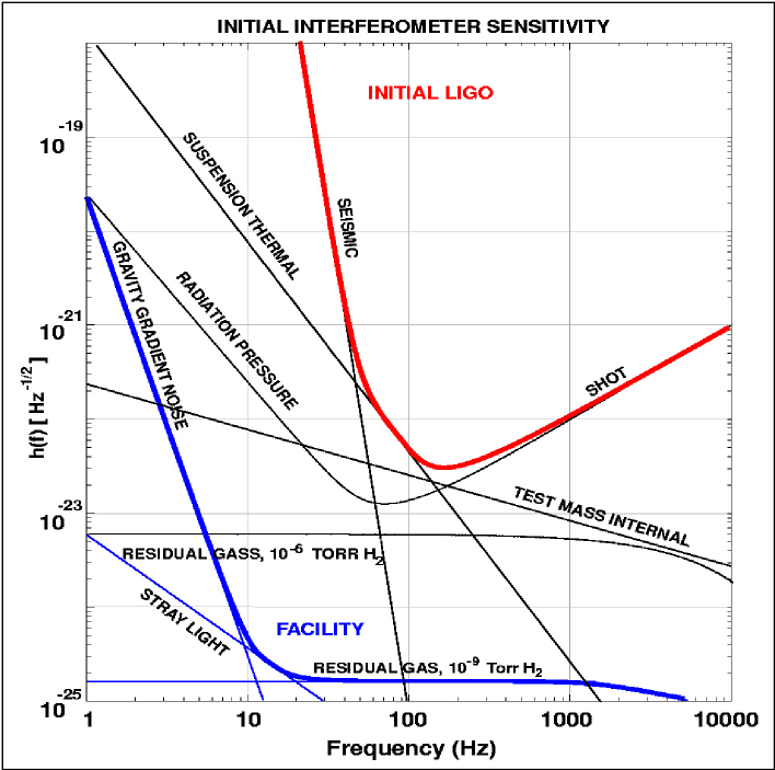
Figure 2: Sensitivity goals of the initial LIGO interferometers, and facility limits on the LIGO sensitivity (taken from Ref. [25]).

We now survey the more well-understood possible sources of measurable GWs in the high-frequency band. We emphasize at this point that such a listing of sources can in no way be considered comprehensive: We are hopeful that some GW sources may surprise us, as has been the case whenever we have studied the Universe with a new type of radiation.

6.1.1 Coalescing compact binaries

Compact binaries — binary star systems in which each member is a neutron star or black hole — are currently the best understood sources of GWs. Double neutron stars have been studied observationally since the mid 1970s; five such systems [12, 13, 14, 15, 16] tight enough to merge within a few $10^{8}$ or $10^{9}$ years have been identified in our Galaxy. Extrapolation from these observed binaries in the Milky Way to the Universe at large [61, 62, 63, 64] indicates that GW detectors should measure at least several and at most several hundred binary neutron star mergers each year (following detector upgrades; the expected rate for initial detectors is of order one event per several years, so that measurement of an event is plausible but of fairly low probability). Population synthesis (modeling evolution of stellar populations) indicates that the measured rate of binaries containing black holes should likewise be interestingly large (perhaps even for initial detectors) [65, 66, 67, 68]. The uncertainties of population synthesis calculations are rather large, however, due to poorly understood aspects of stellar evolution and compact binary formation; data from GW detectors is likely to have a large impact on this field.

6.1.2 Stellar core collapse

Core collapse in massive stars (the engine of Type II supernova explosions) has long been regarded as likely to be an important source of GWs; see, for example, Ref. [69] for an early review. Stellar collapse certainly exhibits all of the necessary conditions for strong GW generation — large amounts of mass ($1-100\,M_{\odot}$) flow in a compact region (hundreds to thousands of kilometers) at relativistic speeds ($v/c\;\hbox to0.0pt{\lower 2.5pt\hbox{$\sim$}\hss}\raise 1.5pt\hbox{$>$}\;1/5$). However, these conditions are not sufficient to guarantee strong emission. In particular, the degree of asymmetry in collapse is not particularly well understood.

If the core of a star is very rapidly rotating during collapse, then instabilities may develop which lead to strong GW emission [70]. If such instabilities develop, core collapse GWs could be detected from events as far away as 10 Megaparsecs [71], a distance encompassing enough galaxies that several events per year would be likely. Most models of massive stars, however, indicate that such rapid rotation is not likely (e.g., [72]). Even without the growth of instabilities, the asymmetric dynamics of core collapse is likely to lead to wave emission which would be detectable within the Local Group of galaxies, with perhaps an event every few years detectable by advanced interferometers [73]. The wave strength is likely to correlate strongly with the degree of asymmetry in the supernova. If the GW event has an electromagnetic or neutrino counterpart we may gain a wealth of knowledge regarding the state of the precollapse core [74].

6.1.3 Periodic emitters

Periodic sources of GWs radiate at constant or nearly constant frequency, like radio pulsars. In fact, the prototypical source of continuous GW is a rotating neutron star, or GW pulsar. A non-axisymmetry in a neutron star crust (caused, for example, by an oblateness that is misaligned with the star’s spin axis) will radiate GWs with characteristic amplitude

$$h\sim{G\over c^{4}}{If^{2}\epsilon\over r}\;.$$ (6.2)

Here $I$ is the star’s moment of inertia, $f$ is the wave frequency, $r$ is the distance to the source, and $\epsilon$ is the dimensionless fractional distortion $\epsilon=(I_{xx}-I_{yy})/I$, where $I_{ij}$ is the moment of inertia tensor. The crucial parameter $\epsilon$ characterizes the degree to which the star is distorted; it is rather poorly understood. Upgraded interferometers in LIGO could set an upper limit on $\epsilon$ of order $10^{-6}$ for sources at $\sim 10$ kpc [27]. Various mechanisms have been proposed to explain how a neutron star can be distorted to give a value of $\epsilon$ that is interesting as a GW source; see [75, 76] for further discussion. Examples of some interesting mechanisms include misalignment of a star’s internal magnetic field with the rotation axis [77] and distortion by accreting material from a companion star [78, 79] (discussed in more detail below).

Whatever the mechanism generating the distortion, it is clear that $\epsilon$ will be small, so that $h\sim 10^{-24}$ or smaller — quite weak. Measuring these waves will require coherently tracking their signal for a large number of wave cycles. Coherently tracking $N$ cycles boosts the signal to noise ratio by a factor $\sim\sqrt{N}$. This is actually fairly difficult, since the signal is strongly modulated by the Earth’s rotation and orbital motion, “smearing” the waves’ power across multiple frequency bands. Searching for periodic GWs means demodulating the motion of the detector, a computationally intensive problem since the modulation is different for every sky position. Unless one knows in advance the position of the source, one needs to search over a huge number of sky position “error boxes”, perhaps as many as $10^{13}$. One rapidly becomes computationally limited. (Radio pulsar searches face this same problem, with the additional complication that radio pulses are dispersed by the interstellar medium. However, radio observers usually use shorter integration times, and often target their searches on small regions of the sky, so their computational cost is usually not as great.) For further discussion, see [80]; for ideas about doing hierarchical searches that require less computer power, see [81].

As mentioned above, one particularly interesting mechanism for distorting a neutron star comes from accretion of material from a companion star. Accretion provides a spin-up torque to a neutron star,

$$\left(dJ/dt\right)_{\rm spin-up}\sim R^{2}\Omega_{*}\dot{M}$$ (6.3)

(where $J$ is the spin angular momentum, $\Omega_{*}$ is the orbital frequency of the accreting matter as it plunges onto the star, $R$ is the star’s radius, and $\dot{M}$ is the mass accretion rate). Without any kind of braking mechanism, the neutron star would presumably spin-up until it reaches the “breakup limit”, i.e., the spin frequency at which centrifugal forces would begin to break it apart; the breakup frequency is typically around 2000 – 3000 Hz.

Observations have shown [82] that accreting neutron stars do, in fact, appear to have a “speed limit” — no accreting neutron star has been observed to spin faster than 619 Hz [83]. This is consistent with the fact that the fastest radio pulsar has a spin period of 641 Hz [84]. This suggest that some mechanism is removing angular momentum from the neutron star. A plausible and very attractive possibility for how this angular momentum is removed is via GW emission. Because the spin-down torque due to GW emission grows sharply with spin frequency,

$$\left(dJ/dt\right)_{\rm spin-down}\propto\Omega^{5}\quad\mbox{(Quadrupole emission)}\;,$$ (6.4)

the limiting spin obtained by balancing the torques (6.3) and (6.4) is relatively insensitive to the mass accretion rate ${\dot{M}}$. Such a mechanism was originally suggested by Wagoner [85], and was revived by Bildsten [78] to explain the narrow clustering in spin frequency of accreting low-mass x-ray binaries (LMXBs). Various mechanisms could provide the spin-down torque — Bildsten originally suggested a quadrupole moment in the spinning star could be induced by a thermally varying electron capture mechanism, but also noted that the r-mode instability (see, e.g., [86] for a review) could be excited, leading to a similar spin-down law. Whatever the mechanism, accreting neutron stars are obvious and very attractive targets for observing campaigns with GW detectors, particularly given that their sky positions are well known.

6.1.4 Stochastic backgrounds

Stochastic backgrounds are “random” GWs, arising from a large number of independent, uncorrelated sources that are not individually resolvable. A particularly interesting source of stochastic waves is the dynamics of the early Universe, which could produce an all-sky GW background, similar to the cosmic microwave background; see Refs. [87, 88, 89] for detailed reviews. Stochastic waves can be generated in the early Universe via a variety of mechanisms: amplification of primordial fluctuations in the Universe’s geometry via inflation, phase transitions as previously unified interactions separate, a network of vibrating cosmic strings, or the condensation of a brane from a higher dimensional space. These waves can actually extend over a wide range of frequency bands; waves from inflation in particular span all bands, from ultra low frequency to high frequency.

Stochastic backgrounds are usually idealized as being stationary, isotropic and homogeneous. They are thus characterized by their energy density per unit frequency, $d\rho_{\rm gw}/df$. This is often parameterized in terms of the energy density per unit logarithmic frequency divided by the critical energy density to close the Universe

$$\Omega_{\rm gw}(f)={1\over\rho_{\rm crit}}{d\rho_{\rm gw}\over d\ln f}\;,$$ (6.5)

where $\rho_{\rm crit}=3H_{0}^{2}/8\pi G$ is the critical density and $H_{0}$ is the value of the Hubble constant today. Different cosmological sources produce different levels of $\Omega_{\rm gw}(f)$, centered in different bands. In the high frequency band, waves produced by inflation are likely to be rather weak: estimates suggest that the spectrum will be flat across LIGO’s band, with magnitude $\Omega_{\rm gw}\sim 10^{-15}$ at best [90]. Waves from phase transitions can be significantly stronger, but are typically peaked around a frequency that depends on the temperature $T$ of the phase transition [87, 91]:

$$f_{\rm peak}\sim 100\,{\rm Hz}\left({T\over 10^{5}\,{\rm TeV}}\right)\;.$$ (6.6)

Because of their random nature, stochastic GWs look just like noise. Ground-based detectors will measure stochastic backgrounds by comparing data at multiple sites and looking for “noise” that is correlated [88, 92]. For comparing to a detector’s noise, one should construct the characteristic stochastic wave strain,

$$h\propto f^{-3/2}\sqrt{\Omega_{\rm gw}(f)\Delta f}\;,$$ (6.7)

where $\Delta f$ is the frequency band across which the measurement is made. For further discussion and the proportionality constants, see [88]. Note that if $\Omega_{\rm gw}(f)$ is constant, this strain level grows sharply with decreasing frequency — the most interesting limits are likely to be set by measurements at low frequencies.

Early detectors will have fairly poor sensitivity to the background, constraining it to a level $\Omega_{\rm gw}\sim 5\times 10^{-6}$ in a band from about 100 Hz to 1000 Hz. This is barely more sensitive than known limits from cosmic nucleosynthesis [87]. Later upgrades will be significantly more sensitive, able to detect waves with $\Omega_{\rm gw}\sim 10^{-10}$, which is good enough to place interesting limits on backgrounds from some phase transitions.

6.2 Low frequency

There is no hope of measuring GWs in the low frequency band, $10^{-5}\,{\rm Hz}\;\hbox to0.0pt{\lower 2.5pt\hbox{$\sim$}\hss}\raise 1.5pt\hbox{$<$}\;f\;\hbox to0.0pt{\lower 2.5pt\hbox{$\sim$}\hss}\raise 1.5pt\hbox{$<$}\;1\,{\rm Hz}$, using a ground-based instrument: Even if it were possible to completely isolate one’s instrument from local ground motions, gravitational coupling to fluctuations in the local mass distribution ultimately limits the sensitivity to frequencies $f\;\hbox to0.0pt{\lower 2.5pt\hbox{$\sim$}\hss}\raise 1.5pt\hbox{$>$}\;1\,{\rm Hz}$. Nonetheless, many extremely interesting sources radiate in this band. The only way to measure these waves is to build a detector in the quiet environment of space, far removed from low-frequency noise sources.

Such an instrument is currently being designed jointly by NASA in the United States and ESA, the European Space Agency: LISA, the Laser Interferometer Space Antenna. If all goes well, LISA will be launched into orbit in 2013 or so. LISA will be a laser interferometer, similar in concept to the ground-based detectors: Changes in the distance between widely separated test masses will be monitored for GWs. However, LISA’s scale is vastly larger than that of its ground-based cousins, and so details of its operations are quite different. In particular, LISA will have armlengths $L\simeq 5\times 10^{6}\,{\rm km}$. The three spacecraft which delineate the ends of LISA’s arms are placed into orbits such that LISA forms a triangular constellation orbiting the sun, inclined $60^{\circ}$ with respect to the plane of the ecliptic and following the Earth with a $20^{\circ}$ lag. This configuration is sketched in Fig. 3. Since it essentially shares Earth’s orbit, the constellation orbits the sun once per year, “rolling” as it does so. This motion plays an important role in pinpointing the position of sources by modulating the measured waveform — the modulation encodes source location and makes position determination possible.

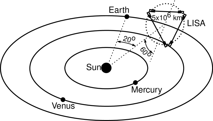
Figure 3: Orbital configuration of the LISA antenna.

The 3 spacecraft each contain two optical assemblies, each of which houses a 1 Watt laser and a 30 centimeter telescope. Because of the extreme lengths of the interferometer’s arms, Fabry-Perot interferometry as in the ground-based detectors is not possible: Diffraction spreads the laser beam over a diameter of about $20\,{\rm km}$ as it propagates from one spacecraft to the other. A portion of that $20\,{\rm km}$ wavefront is sampled with the telescope. That light is then interfered with a sample of light from the on-board laser. Each spacecraft thus generates two interference data streams; six signals are generated by the full LISA constellation. From these six signals, we can construct the time variations of LISA’s armlengths and then build both GW polarizations. More information and details can be found in [93].

Note that the LISA armlengths are not constant — as the constellation orbits, the distances between the various spacecraft vary by about $1\%$ (including effects such as planetary perturbations). These variations are far larger than the displacements produced by GWs, which are of order picometers. However, these variations occur over timescales of order months, and are extremely smooth and well modeled. It will not be difficult to remove them from the data leaving clean data in the interesting frequency band. Picometer scale variations are not too difficult to measure in this band by gathering photons for a time $10\,{\rm sec}\;\hbox to0.0pt{\lower 2.5pt\hbox{$\sim$}\hss}\raise 1.5pt\hbox{$<$}\;T\;\hbox to0.0pt{\lower 2.5pt\hbox{$\sim$}\hss}\raise 1.5pt\hbox{$<$}\;1\,{\rm day}$. Even though the bulk of the laser’s emitted power is lost by diffraction, enough photons are gathered on this timescale that the phase shift due to the GW can be determined.

The GW signals are actually read out by monitoring the position of the so-called “gravitational sensor” on each optical assembly; in particular, the position of a “proof mass” which floats freely and constitutes the test mass for the LISA antenna is monitored. Because it is freely floating, the proof mass follows a geodesic of the spacetime. Micronewton thrusters keep the bulk spacecraft centered on these proof masses, forcing the craft to follow their average trajectory. In this way, the spacecraft are isolated from low frequency forces that could impact the ability to measure GWs (e.g., variations in solar radiation pressure).

We now take a quick tour through some interesting LISA sources:

6.2.1 Periodic emitters

In the high-frequency band, the source of most periodic GWs is expected to be isolated neutron stars. LISA’s periodic GWs will come primarily from binary star systems in the Milky Way, primarily close white dwarf binaries. Most of these systems do not generate waves strong enough to backreact significantly, so that their frequencies do not change measurably over the course of LISA observations. Certain systems are well-known in advance to be sources of periodic waves for the LISA band. These sources are understood well enough from optical observations that they may be regarded as “calibrators” — LISA had better detect them, or else something is wrong!

Aside from these sources that are known in advance, it is expected that LISA will discover a good number of binary systems that are too faint to detect with telescopes. Joint observations by LISA and other astronomical instruments are likely to be more fruitful than observations with a single instrument alone. For example, it is typically difficult for telescopes to determine the inclination of a binary to the line of sight (a quantity needed to help pin down the masses of the binary’s members). GWs measure the inclination angle almost automatically, since this angle determines the relative magnitude of the polarizations $h_{+}$ and $h_{\times}$.

The total number of periodic binaries radiating in LISA’s band is expected to be so large that they will constitute a confused, stochastic background at low frequencies — there are likely to be several thousand galactic binaries radiating in each resolvable frequency bin. This background will constitute a source of “noise” (from the standpoint of measuring other astrophysical sources) that is largely than that intrinsic to the instrument noise at $f\;\hbox to0.0pt{\lower 2.5pt\hbox{$\sim$}\hss}\raise 1.5pt\hbox{$<$}\;10^{-3}$ Hz.

6.2.2 Coalescing binary systems containing black holes

Coalescing binary black hole systems will be measurable by LISA to extremely large distances — essentially to the edge of the observable Universe. Even if such events are very rare, the observed volume is enormous so an interesting event detection rate is very likely. One class of such binaries consists of systems in which the member holes are of roughly equal mass ($\sim 10^{5}-10^{8}M_{\odot}$). These binaries can form following the merger of galaxies (or pregalactic structures) containing a black holes in their cores. Depending on the mass of the binary, the waves from these coalescences will be detectable to fairly large redshifts ($z\sim 5-10$), possibly probing an early epoch in the formation of the Universe’s structure [94].

The other major class of binary systems consists of relatively small bodies (black holes with mass $\sim 10$ – $100\,M_{\odot}$, neutron stars, or white dwarfs) that are captured by larger black holes ($M\sim 10^{5}-10^{7}\,M_{\odot}$). These “extreme mass ratio” binaries are created when the smaller body is captured onto an extremely strong field, highly relativistic orbit, generating strong GWs. Such systems are measurable to a distance of a few Gigaparsecs if the inspiralling body is a $10\,M_{\odot}$ black hole, and to a distance of a few hundred Megaparsecs if the body is a neutron star or white dwarf. LISA will measure the waves that come from the last year or so of the smaller body’s inspiral, and thence probe the nature of the larger black hole’s gravitational field deep within the hole’s potential. The rates for such events are not too well understood and depend on the details of stellar dynamics in the cores of galaxies. Extremely conservative estimates typically find that the rate of measurable events for LISA should be at least several per year [95, 96]. Recent thinking suggests that these rates are likely to be rather underestimated — black holes (which are measurable to much greater distances) are likely to dominate the measured rate, perhaps increasing the rate to several dozen or several hundred per year [97].

Finally, it is worth noting that many events involving intermediate mass black holes — those with masses in the band running from a few $10^{2}$ to a few $10^{5}\,M_{\odot}$ — would generate GWs in LISA’s sensitive band. There is a large body of tentative evidence for the existence of black holes in this mass band (see, e.g., [98] for a review), though as yet we have no “smoking gun” unambiguous signature for such a hole. If such black holes do exist and undergo mergers in sufficient numbers, measurement of their waves will make possible a wealth of interesting tests of relativity [99], and could untangle some of the mysteries surrounding supermassive black hole formation and growth.

6.2.3 Stochastic backgrounds

As discussed in Sec. 6.1.4, ground-based detectors can measure a stochastic background by correlating the data streams of widely separated detectors. LISA will use a slightly different technique: by combining its six data streams in an appropriate way, one can construct an observable that is completely insensitive to GWs, measuring noise only [100]. This makes it possible to distinguish between a noise-like stochastic background and true instrumental noise, and thereby to learn about the characteristics of the background [101].

The sensitivity of LISA will not be good enough to set interesting limits on an inflationary GW background: LISA will only reach $\Omega_{\rm gw}\sim 10^{-11}$, about four orders of magnitude too large to begin to say something about inflation [90]. However, LISA’s band is well placed for other possible sources of cosmological backgrounds. In particular, an electroweak phase transition at temperature $T\sim 100-1000$ GeV would generate waves in LISA’s band [cf. Eq. (6.6)]. These waves are likely to be detectable if the phase transition is strongly first order (a scenario that does not occur in the standard model, but is conceivable in extensions to the standard model [91]).

6.3 Very low frequency

The very low frequency band, $10^{-9}\,{\rm Hz}\;\hbox to0.0pt{\lower 2.5pt\hbox{$\sim$}\hss}\raise 1.5pt\hbox{$<$}\;f\;\hbox to0.0pt{\lower 2.5pt\hbox{$\sim$}\hss}\raise 1.5pt\hbox{$<$}\;10^{-7}\,{\rm Hz}$, corresponds to waves with periods ranging from a few months to a few decades. Our best limits on waves in this band come from observations of millisecond pulsars. First suggested by Sazhin [102] and then carefully analyzed and formulated by Detweiler [103], GWs can drive oscillations in the arrival times of pulses from a distant pulsar. Millisecond pulsars are very good “detectors” for measurements in this band because they are exquisitely precise clocks. The range of frequencies encompassed by the very low frequency band is set by the properties of these radio pulsar measurements: the high end of the frequency band comes from the need to integrate the radio pulsar data for at least several months; the low end comes from the fact that we have only been observing millisecond pulsars for a few decades. (One cannot observe a periodicity shorter than the span of one’s dataset.) A recent upper limit derived from this technique is [104]

$$\Omega_{\rm gw}h_{100}^{2}<9.3\times 10^{-8},\ \ \ \ \ 4\times 10^{-9}~{}{\rm Hz}<f<4\times 10^{-8}~{}{\rm Hz}$$ (6.8)

(where the limit is a $95\%$ confidence limit and $h_{100}$ is the Hubble constant in units of $100\,{\rm km}\,{\rm sec}^{-1}\,{\rm Mpc}^{-1}$).

The upper limit (6.8) already places constraints on some cosmological models (in particular those involving cosmic strings). With further observations and the inclusion of additional pulsars in the datasets, it is likely to improve quite soon. It is possible that the background in this band will be dominated by many unresolved coalescing massive binary black holes [105] — binaries that are either too massive to radiate in the LISA band, or else are inspiralling towards the LISA band en route to a final merger several centuries or millenia hence. Constraints from pulsar observations in this band will remain an extremely important source of data on stochastic waves in the future — the limits they can set on $\Omega_{\rm gw}$ are likely to be better than can be set by any of the laser interferometric detectors.

6.4 Ultra low frequency

The ultra low frequency band, $10^{-18}\,{\rm Hz}\;\hbox to0.0pt{\lower 2.5pt\hbox{$\sim$}\hss}\raise 1.5pt\hbox{$<$}\;f\;\hbox to0.0pt{\lower 2.5pt\hbox{$\sim$}\hss}\raise 1.5pt\hbox{$<$}\;10^{-13}\,{\rm Hz}$, is better described by converting from frequency to wavelength: For these waves, $10^{-5}\,H_{0}^{-1}\;\hbox to0.0pt{\lower 2.5pt\hbox{$\sim$}\hss}\raise 1.5pt\hbox{$<$}\;\lambda\;\hbox to0.0pt{\lower 2.5pt\hbox{$\sim$}\hss}\raise 1.5pt\hbox{$<$}\;H_{0}^{-1}$, where $H_{0}^{-1}\sim 10^{10}$ light years is the Hubble length today. Waves in this band oscillate on scales comparable to the size of the Universe. They are most likely to be generated during inflation: Quantum fluctuations in the spacetime metric are parametrically amplified during inflation to relatively high amplitude. The rms amplitude to which the waves are amplified depends upon the energy scale $E_{\rm infl}$ of inflation:

$$h_{\rm rms}\propto\left(E_{\rm infl}\over m_{\rm P}\right)^{2}\;,$$ (6.9)

where $m_{\rm P}$ is the Planck mass. Measuring these GWs would be a direct probe of inflationary physics, and would determine the inflation energy scale, which is currently unknown to within many orders of magnitude. These waves have been described as the “smoking gun” signature of inflation [106].

During inflation, quantum fluctuations impact both the scalar field which drives inflation (the inflaton $\phi$) and the metric of spacetime. There exist independent scalar fluctuations (coupled fluctuations in the inflaton and scalar-type fluctuations in the metric) and tensor fluctuations (tensor-type fluctuations in the metric). The Fourier modes of these scalar and tensor perturbations are describable as harmonic oscillators in the expanding Universe [107]. Each mode undergoes zero-point oscillations in the harmonic potential. However, the potential itself is evolving due to the expansion of the Universe. The evolution of this potential parametrically amplifies these zero-point oscillations, creating quanta of the field [87]. During inflation, the Universe’s scale factor $a(t)$ grows faster than the Hubble length $H^{-1}$, and so each mode’s wavelength likewise grows faster than the Hubble length. The mode’s wavelength eventually becomes larger than the Hubble length, or the mode “leaves the horizon”. After inflation ends the mode subsequently renters the horizon. For gravitational perturbations the number of quanta generated in the mode is proportional to the factor by which the Universe expands between the two different horizon crossings. Fluctuations in the inflaton seed density fluctuations, $\delta\rho(\vec{r})=\delta\phi(\vec{r})(\partial V/\partial\phi)$ [where $V(\phi)$ is the potential that drives the inflaton field]. The tensor-type fluctuations in the spacetime metric are GWs.

Density fluctuations and GWs both leave an imprint upon the cosmic microwave background (CMB). First, each contributes to the CMB temperature anisotropy. However, even a perfectly measured map of temperature anisotropy cannot really determine the contribution of GWs very well because of cosmic variance: Since we only have one Universe to observe, we are sharply limited in the number of statistically independent influences upon the CMB that we can measure. Large angular scales are obviously most strongly affected by this variance, and these scales are the ones on which GW most importantly impact the CMB [108].

Fortunately, the scalar and tensor contributions also impact the polarization of the CMB. These two contributions can be detangled from one another in a model-independent fashion. This detangling uses the fact that the polarization tensor $P_{ab}({{\bf\hat{n}}})$ on the celestial sphere can be decomposed into tensor harmonics. These harmonics come in two flavors, distinguished by their parity properties: The “E-modes” or “gradient-type” harmonics $Y_{(lm)ab}^{E}({\bf\hat{n}})$ [which pick up a factor $(-1)^{l}$ under ${\bf\hat{n}}\to-{\bf\hat{n}}$], and the “B-modes” or “curl-type” harmonics $Y_{(lm)ab}^{C}({\bf\hat{n}})$ [which pick up a factor $(-1)^{l+1}$ under ${\bf\hat{n}}\to-{\bf\hat{n}}$]. These harmonics are constructed by taking covariant derivatives on the sphere of the “ordinary” spherical harmonics $Y_{lm}({\bf\hat{n}})$; see [109] for details. Because scalar perturbations have no handedness, they only induce gradient-type polarization. GWs induce both gradient- and curl-type polarization. Thus, an unambiguous detection of the curl-type polarization would confirm production of GWs by inflation. (A caveat is that is that gravitational lensing can convert E-modes to B-modes; this so-called “cosmic shear” ultimately limits the sensitivity to GWs of CMB polarization studies [110].)

7 Conclusion

This article has summarized many of the most important topics in the theory of GWs. Due to space and time limitations, we sadly were not able to cover all topics with which students of this field should be familiar. In particular, we had hoped to include a discussion of strong field relativity and GW emission. We confine ourselves, in this conclusion, to a (very) brief discussion of important aspects of this subject for GW science, as well as pointers to the relevant literature.

Linearized theory as described in Secs. 2 and 5 is entirely adequate to describe the propagation of GWs through our Universe and to model the interaction of GWs with our detectors. In some cases, it is even adequate to describe the emission of waves from a source, as described in Sec. 4 (although for sources with non-negligible self gravity such as binary star systems one has to augment linearized theory as described in Sec. 4.2). However, many sources have very strong self gravity where the linearized treatment is completely inadequate. A variety of formalisms have been developed to handle these cases.

• Post-Newtonian (PN) theory. PN theory is one of the most important of these formalisms, particularly for modeling binary systems. Roughly speaking, PN theory analyzes sources using an iterated expansion in two variables: The “gravitational potential”, $\phi\sim M/r$, where $M$ is a mass scale and $r$ characterizes the distance from the source; and velocities of internal motion, $v$. (In linearized theory, we assume $\phi$ is small but place no constraints on $v$.) Newtonian gravity emerges as the first term in the expansion, and higher order corrections are found as the expansion is iterated to ever higher order. Our derivation of the quadrupole formula in Sec. 4.2 gives the leading order term in the PN expansion of the emitted radiation. See Luc Blanchet’s recent review [111] and references therein for a comprehensive introduction to and explication of this subject.

• Numerical relativity. Numerical relativity seeks to directly integrate Einstein’s equations on a computer. Ideally, we would like to to use a well-understood model of a GW source (e.g., a binary system in which the field strengths are small enough that it is well described by post-Newtonian theory) as “initial data”, and then numerically evolve the Einstein equations from that point to some final equilibrium configuration. The form in which we normally encounter Einstein’s equation in textbooks is not well suited to this task — the coordinate freedom of general relativity means that there is no notion of “time” built into the equation $G_{ab}=8\pi T_{ab}$. One must introduce some notion of time for the concept of “initial data” to have any meaning. The 4 dimensions of spacetime are then split into 3+1 dimensions of space and time. Having made this choice, Einstein’s equations take on a particular form which is amenable to numerical computation.

  A detailed discussion of numerical relativity is given in the contribution by Choptuik to this volume [112]; we also recommend the reviews by Lehner [113] and by Baumgarte and Shapiro [37]. For the purpose of our present discussion, it suffices to remark that it has proven to be extremely difficult to model some of the most interesting and important GW sources. In particular, the final stage of binary black hole mergers — regarded by many as the “Holy Grail” of numerical relativity — has proven to be quite a challenge.

• Perturbation theory. In some cases, GW sources can be modeled as nearly, but not quite, identical to some exact solution of the Einstein field equations. For example, the end state of binary black hole coalescence must be a single black hole. As we approach this final state, the system will be well-modeled as the Kerr black hole solution, plus some distortion that radiates away. Another example is a binary consisting of a stellar mass compact body orbiting a massive black hole. The binary’s spacetime will be well-described as a single black hole plus a perturbation due to the captured body. These cases can be nicely described using perturbation theory: We treat the spacetime as some exact background, $g_{ab}^{\rm B}$, plus a perturbation $h_{ab}$:

  $$g_{ab}=g^{\rm B}_{ab}+h_{ab}\;.$$ (7.1)

  We are in the perturbative regime if $||h_{ab}||/||g^{\rm B}_{ab}||\ll 1$. This system can then be analyzed by expanding the Einstein equations for this metric and keeping terms to first order in $h_{ab}$ (see Sec. 5.1 for details but without the matter source terms included).

  This approach has proven to be particularly fruitful when the background spacetime is that of a black hole. For the case of a Schwarzschild background, the derivation of the full perturbation equations is rather straightforward; Rezzolla gives a particularly compact and readable summary [114]. Perturbations of Kerr black holes are not nearly so simple to describe, largely due to the lack of spherical symmetry — expanding the metric as in Eq. (7.1) does not prove to be so fruitful as it is in the Schwarzschild case. Somewhat miraculously, it turns out that progress can be made by expanding the curvature tensor: By expanding the Riemann tensor as $R_{abcd}=R^{\rm B}_{abcd}+\delta R_{abcd}$ and taking an additional derivative of the Bianchi identity,

  $$\nabla_{e}R_{abcd}+\nabla_{d}R_{abec}+\nabla_{c}R_{abde}=0\;,$$ (7.2)

  one can derive a wave-like equation for the perturbation $\delta R_{abcd}$. This analysis was originally performed by Teukolsky; see his original analysis [115] for details.

Appendix A Existence of TT gauge in local vacuum regions in linearized gravity

In this appendix we show that one can always find TT gauges in local vacuum regions in linearized gravity. More precisely, suppose that ${\cal V}$ is a connected open spatial region, and $(t_{0},t_{1})$ is an open interval of time. Then one can find a gauge on the product ${\cal R}\equiv(t_{0},t_{1})\times{\cal V}$ that satisfies $h_{tt}=h_{ti}=\delta^{ij}h_{ij}=\partial_{i}h_{ij}=0$, as long as $T_{ab}=0$ throughout ${\cal R}$.

The proof involves a generalization of the gauge-invariant formalism of Sec. 2.2 to finite spacetime regions. We define a decomposition of the metric perturbation $h_{ab}$ in terms of quantities $\phi$, $\beta_{i}$, $\gamma$, $h_{ij}^{\rm TT}$, $H$, $\varepsilon_{i}$ and $\lambda$ using the same equations (2.29) – (2.35) as before. However we replace the boundary conditions (2.36) with

$$\gamma_{|\partial{\cal V}} = \int_{t_{0}}^{t}dt\,\phi_{|\partial V},$$ (1.1)

$$\lambda_{|\partial{\cal V}} = 0,$$ (1.2)

$$(\nabla^{2}\lambda)_{|\partial{\cal V}} = H_{|\partial{\cal V}},$$ (1.3)

$$({\bf n}\times{\mbox{\boldmath$\varepsilon$}})_{|\partial{\cal V}} = 2\int_{t_{0}}^{t}dt\,({\bf n}\times{\mbox{\boldmath$\beta$}})_{|\partial{\cal V}},$$ (1.4)

where ${\bf n}$ is the unit outward-pointing unit normal to $\partial{\cal V}$. The reason for this particular choice of boundary conditions will be explained below. These boundary conditions define a unique decomposition of the metric within ${\cal R}$.

Next, we compute how the variables $\phi$, $\beta_{i}$, $\gamma$, $h_{ij}^{\rm TT}$, $H$, $\varepsilon_{i}$ and $\lambda$ transform under general gauge transformations. We use the same parameterization (2.37) of the gauge transformation as before, except we impose now the boundary condition $C_{|\partial{\cal V}}=0$. We find that the transformation laws (2.38) – (2.44) are replaced by the following equations which contain some extra terms:

$$\phi \to \quad\phi-\dot{A}\;,$$ (1.5)

$$\beta_{i} \to \quad\beta_{i}-\dot{B}_{i}-\partial_{i}\psi\;,$$ (1.6)

$$\gamma \to \quad\gamma-A-\dot{C}+\psi\;,$$ (1.7)

$$H \to \quad H-2\nabla^{2}C\;,$$ (1.8)

$$\lambda \to \quad\lambda-2C\;,$$ (1.9)

$$\varepsilon_{i} \to \quad\varepsilon_{i}-2B_{i}+2\eta_{i}-2(t-t_{0})\partial_{i}\psi\;,$$ (1.10)

$$h_{ij}^{\rm TT} \to \quad h_{ij}^{\rm TT}-2\partial_{(i}\eta_{j)}+2(t-t_{0})\partial_{i}\partial_{j}\psi\;.$$ (1.11)

Here $\psi$ is the time-independent, harmonic function defined by $\nabla^{2}\psi=0$ and $\psi_{|\partial{\cal V}}=A_{|\partial{\cal V},t=t_{0}}$. Similarly $\eta_{i}$ is the time-independent, harmonic transverse vector defined by $\nabla^{2}\eta_{i}=0$ and $({\bf n}\times{\mbox{\boldmath$\eta$}})_{|\partial{\cal V}}={\bf n}\times{\bf B}_{|\partial{\cal V},t=t_{0}}.$

We define the variables $\Phi$, $\Theta$ and $\Xi_{i}$ by the same equations (2.45) – (2.47) as before. From the transformation laws (1.5) – (1.11) these variables are still gauge invariant, while $h_{ij}^{\rm TT}$ is no longer gauge invariant in the present context. Next, imposing the linearized vacuum Einstein equations using the expressions (2.59) – (2.2) yields

$$\nabla^{2}\Theta=0,\ \ \ \ \nabla^{2}\Xi_{i}=-2\partial_{i}{\dot{\Theta}},\ \ \ \ \nabla^{2}\Phi=\frac{3}{2}{\ddot{\Theta}}$$ (1.12)

in ${\cal V}$. The boundary conditions (1.1) – (1.4) together with the definitions (2.45) – (2.47) imply that the boundary conditions on the gauge invariant variables are

$$\Phi_{|\partial{\cal V}}=\Theta_{|\partial{\cal V}}=\Xi^{i}_{|\partial{\cal V}}=0.$$ (1.13)

(This is why we choose those particular boundary conditions.) Therefore all the gauge invariant variables vanish, $\Theta=\Phi=\Xi^{i}=0$ in ${\cal R}$.

It is now straightforward to show that one can choose a gauge in which $\phi=\beta_{i}=\gamma=H=\varepsilon_{i}=\lambda=0$. From the transformation laws (1.5) – (1.11) we can choose $C$ to make $\lambda=0$, choose ${\dot{A}}$ to make $\phi=0$, and choose ${\dot{B}}_{i}$ to make $\beta_{i}=0$. The residual gauge freedom is then parameterized by functions $A$ and $B_{i}$ that are time-independent. Next, from Eq. (1.13) together with the definitions (2.45) – (2.47) it follows that

$$0 = \Theta=\frac{1}{3}H$$ (1.14)

$$0 = \Phi=-2{\dot{\gamma}}$$ (1.15)

$$0 = \Xi_{i}=-\frac{1}{2}{\dot{\varepsilon}}_{i}.$$ (1.16)

Thus the only remaining non-zero pieces of the metric other than the TT piece are $\gamma$ and $\varepsilon_{i}$, and these are both time-independent. Finally we can use the residual gauge freedom given by time-independent functions $A$ and $B_{i}$ to set to zero $\gamma$ and $\varepsilon_{i}$, by Eqs. (1.7) and (1.10). [For this purpose $A$ and $B_{i}$ will vanish on $\partial{\cal V}$, by Eqs. (1.1) and (1.4), so $\psi$ and $\eta_{i}$ vanish.]

References

References

- [1] A. Einstein, “On the electrodynamics of moving bodies”, Annalen Phys. 17, 891 (1905).
- [2] I. Newton, “Philosophiae naturalis principia mathematica” (2nd ed., Streater, London, 1687); from the General Scholum added at the end of the 3rd book in the 2nd edition of 1713.
- [3] I. Newton, “Philosophiae naturalis principia mathematica” (1st ed., Streater, London, 1687). All quotes from the Principia are taken from Ref. [4], Box 1.10.
- [4] C. W. Misner, K. S. Thorne, and J. A. Wheeler, “Gravitation” (Freeman, San Francisco, 1973).
- [5] A. Einstein, “On the general theory of relativity”, Sitzungsberichte Preußische Akademie der Wissenschaften Berlin (Math. Phys.) 778 (1915); 799 (1915).
- [6] A. Einstein, “On the field equations of gravitation”, Sitzungsberichte Preußische Akademie der Wissenschaften Berlin (Math. Phys.) 844 (1915).
- [7] B. F. Schutz, “Gravitational waves on the back on an envelope”, Am. J. Phys. 52, 412 (1984).
- [8] A. Einstein, “Approximative integration of the field equations of gravitation”, Sitzungsberichte Preußische Akademie der Wissenschaften Berlin (Math. Phys.) 688 (1916).
- [9] A. Einstein, “On gravitational waves”, Sitzungsberichte Preußische Akademie der Wissen-schaften Berlin (Math. Phys.) 154 (1918).
- [10] D. Kennefick, “Controversies in the history of the radiation reaction problem in general relativity”, unpublished Ph. D. thesis (Part II), California Institute of Technology (1997); short version available as gr-qc/9704002.
- [11] R. A. Hulse and J. H. Taylor, “Discovery of a pulsar in a binary system”, Astrophys. J. 195, L51 (1975).
- [12] J. M. Weisberg and J. H. Taylor, “Relativistic Binary Pulsar B1913+16: Thirty Years of Observations and Analysis”, to be published in “Binary Radio Pulsars”, to be published in Proc. Aspen Conference, ASP Conf. Series, eds. F. A. Rasio and I. H. Stairs; astro-ph/0407149.
- [13] I. H. Stairs, S. E. Thorsett, J. H. Taylor, and A. Wolszczan, “Studies of the Relativistic Binary Pulsar PSR B1534+12. I. Timing Analysis”, Astrophys. J. 581, 501 (2002).
- [14] W. T. S. Deich and S. R. Kulkarni, “The Masses of the Neutron Stars in M15C”, in “Compact stars in binaries”, Proc. IAU symposium 165, eds. J. van Paradijs, E. P. J. van den Heuvel, and E. Kuulkers (Kluwer Academic Publishers, Dordrecht, 1996), p. 279.
- [15] M. Burgay et al, “An increased estimate of the merger rate of double neutron stars from observations of a highly relativistic system”, Nature 426, 531 (2003).
- [16] A. J. Faulker et al, “ PSR J1756-2251: a new relativistic double neutron star system”, to be published in the Astrophys. J.; astro-ph/0411796.
- [17] B. Abbott et al, “Setting upper limits on the strength of periodic gravitational waves from PSR J1939+2134 using the first science data from the GEO 600 and LIGO detectors”, Phys. Rev. D 69, 082004 (2004).
- [18] B. Abbott et al, “First upper limits from LIGO on gravitational wave bursts”, Phys. Rev. D 69, 102001 (2004).
- [19] B. Abbott et al, “Analysis of LIGO data for gravitational waves from binary neutron stars”, Phys. Rev. D 69, 122001 (2004).
- [20] B. Abbott et al, “Analysis of first LIGO science data for stochastic gravitational waves”, Phys. Rev. D 69, 122004 (2004).
- [21] K. Danzmann, contribution to this volume.
- [22] S. Bonazzola and J.-A. Marck, “Astrophysical sources of gravitational radiation”, Ann. Rev. Nucl. Part. Sci. 44, 655 (1994).
- [23] B. F. Schutz, “Gravitational wave astronomy”, Class. Quantum Grav. 16, A131 (1999).
- [24] L. P. Grishchuk, V. M. Lipunov, K. A. Postnov, M. E. Prokhorov, and B. S. Sathyaprakash, “Gravitational Wave Astronomy: in Anticipation of First Sources to be Detected”, Phys. Uspekhi 44, 1 (2001); Uspekhi Fizicheskikh Nauk 171, 3 (2001); astro-ph/0008481.
- [25] S. A. Hughes, S. Marká, P. L. Bender, and C. J. Hogan, “New physics and astronomy with the new gravitational-wave observatories”, in “Proceedings of the APS / DPF / DPB Summer Study on the Future of Particle Physics (Snowmass 2001)”, (R. Davidson and C. Quigg, Eds.), eConf C010630 (2001) P402; astro-ph/0110349.
- [26] B. F. Schutz, “Lighthouses of Gravitational Wave Astronomy”, in “Lighthouses of the Universe: The Most Luminous Celestial Objects and Their Use for Cosmology”, Proceedings of the MPA/ESO Conference Lighthouses of the Universe, p. 207; gr-qc/0111095.
- [27] C. Cutler and K. S. Thorne, “An Overview of Gravitational-Wave Sources”, to appear in the Proceedings of 16th International Conference on General Relativity and Gravitation (GR16); gr-qc/0204090.
- [28] L. S. Finn, L.S., “Gravitational radiation sources and signatures”, in Dixon, L., ed., Gravity: From the Hubble Length to the Planck Length, Lectures given at the XXVI SLAC Summer Institute on Particle Physics (National Technical Information Service, Springfield, VA, 1999) [also gr-qc/9903107].
- [29] S. A. Hughes, “Listening to the Universe with Gravitational-Wave Astronomy”, Annals Phys. 303, 142 (2003).
- [30] L. P. Grishchuk, “Update on gravitational-wave research”, to appear in “Astrophysics Update”, ed. J. W. Mason (Springer-Praxis, 2004); gr-qc/0305051.
- [31] K. S. Thorne, “The theory of gravitational radiation: an introductory review”, in “Gravitational Radiation”, Eds. N. Deruelle and T. Piran (North Holland, Amsterdam, 1983).
- [32] B. F. Schutz and F. Ricci, “Gravitational Waves, Sources and Detectors”, in “Gravitational Waves”, Eds. I. Ciufolini, V. Gorini, U. Moschella and P. Fré, (Institute of Physics Publishing, Bristol, UK, 2001).
- [33] “Proceedings of the Les Houches School on Astrophysical Sources of Gravitational Waves”, Eds. J.-A. Marck and J.-P. Lasota (Cambridge University Press, Cambridge, 1996).
- [34] “Gravitational Waves”, Eds. I. Ciufolini, V. Gorini, U. Moschella and P. Fré, (Institute of Physics Publishing, Bristol, UK, 2001).
- [35] “Proceedings of the fifth Edoardo Amaldi conference on gravitational waves”, Ed. C. Bradaschia, Class. Quantum Grav. 21 (2004).
- [36] J. B. Hartle, “Gravity: An introduction to Einstein’s general relativity” (Addison-Wesley, San Francisco, 2003).
- [37] T. W. Baumgarte and S. L. Shapiro, “Numerical relativity and compact binaries”, Phys. Rep. 376, 41 (2003).
- [38] J. Van Bladel, “Lorenz or Lorentz?”, IEEE Antennas Prop. Mag. 33, 69 (1991).
- [39] D. J. Griffiths, “Introduction to Electrodynamics, Third Edition” (Prentice-Hall, Inc., New Jersey, 1999). Note, the footnote on “Lorenz vs. Lorentz” does not appear in the 1st printing, but does appear in the 4th printing.
- [40] A. S. Eddington, “The propagation of gravitational waves”, Proc. R. Soc. London, Series A, 102, 268 (1922)
- [41] J. M. Bardeen, “Gauge-invariant cosmological perturbations”, Phys. Rev. D 22, 1882 (1980).
- [42] E. Bertschinger, “Gravitation in the weak-field limit”, Physics 8.962 (MIT’s general relativity course) lecture notes, Spring 1999.
- [43] S. L. Larson, W. A. Hiscock, and R. W. Hellings, “Sensitivity curves for spaceborne gravitational wave interferometers”, Phys. Rev. D 62, 062001 (2000).
- [44] A. Abramovici et al, Science 256, 325 (1992).
- [45] K. S. Thorne, in 300 years of gravitation, edited by S. W. Hawking and W. Israel (Cambridge University Press, Cambridge, 1987), p. 330.
- [46] S. A. Hughes and K. S. Thorne, “Seismic gravity-gradient noise in interferometric gravitational-wave detectors”, Phys. Rev. D 58 (1998), 122002.
- [47] K. S. Thorne and C. J. Winstein, “Human gravity-gradient noise in interferometric gravitational-wave detectors”, Phys. Rev. D 60 (1999), 082001.
- [48] T. Creighton, “Tumbleweeds and airborne gravitational noise sources for LIGO”, Phys. Rev. D, submitted; gr-qc/0007050.
- [49] J. D. Jackson, “Classical Electrodynamics, Second Edition” (John Wiley & Sons, New York, 1975), Sec. 6.6; or, “Classical Electrodynamics, Third Edition”, (John Wiley & Sons, New York, 1999), Sec. 6.4.
- [50] K. S. Thorne, R. H. Price, and D. A. MacDonald, “Black Holes: The Membrane Paradigm” (Yale University Press, New Haven, 1986).
- [51] R. M. Wald, General Relativity (University of Chicago Press, Chicago, 1984).
- [52] L. P. Grischuk, Nuovo Cimento, Lett. 12, 60 (1975); E. W. Kolb and M. S. Turner, The Early Universe, (Addison-Wesley, Redwood, CA, 1990) and references therein.
- [53] D. R. Brill and J. B. Hartle, “Method of the self-consistent field in general relativity and its application to the gravitational geon”, Phys. Rev. 135, 271 (1964).
- [54] R. A. Isaacson, “Gravitational radiation in the limit of high frequency. I. The linear ap- proximation and geometrical optics”, Phys. Rev. 166, 1263 (1968); “Gravitational radiation in the limit of high frequency. II. Nonlinear terms and the effective stress tensor”,166, 1272 (1968).
- [55] See www.ligo.caltech.edu
- [56] A. Freise, for the Virgo Collaboration, “Status of Virgo”, gr-qc/0406123.
- [57] H. Lück et al., in Proceedings of the 3rd Edoardo Amaldi Conference (S. Meshkov, Ed.), AIP Conference Proceedings 523, p. 119, Melville, New York, 2000.
- [58] M. Ando et al., “Stable operation of a 300-m laser interferometer with sufficient sensitivity to detect gravitational-wave events within our galaxy”, Phys. Rev. Lett. 86, 3950 (2001).
- [59] K. Kuroda et al., “Large-scale cryogenic gravitational wave telescope”, Int. J. Mod. Phys. D 8, 557 (2000).
- [60] D. McCleland et al., in Proceedings of the 3rd Edoardo Amaldi Conference (S. Meshkov, Ed.), AIP Conference Proceedings 523, p. 140, Melville, New York, 2000.
- [61] R. Narayan, T. Piran, and A. Shemi, “Neutron star and black hole binaries in the Galaxy”, Astrophys. J. 379, L17 (1991).
- [62] E. S. Phinney, “The rate of neutron star binary mergers in the universe - Minimal predictions for gravity wave detectors”, Astrophys. J. 380 (1991), L17.
- [63] V. Kalogera and D. R. Lorimer, “An upper limit on the coalescence rate of double neutron-star binaries in the galaxy”, Astrophys. J. 530, 890 (2000).
- [64] M. Burgay et al, “An increased estimate of the merger rate of double neutron stars from observations of a highly relativistic system”, Nature 426, 531 (2003).
- [65] H. Bethe and G. E. Brown, “Evolution of binary compact objects that merge ”, Astrophys. J. 506, 780 (1998).
- [66] S. F. Portegies-Zwart and L. R. Yungel’son, “Formation and evolution of binary neutron stars”, Astron. Astrophys. 332, 173 (1998).
- [67] S. F. Portegies-Zwart and S. L. W. McMillan, “Black hole mergers in the universe”, Astrophys. J. 528, L17 (2000).
- [68] K. Belczynski, V. Kalogera, and T. Bulik, “ A comprehensive study of binary compact objects as gravitational wave sources: evolutionary channels, rates, and physical properties”, Astrophys. J. 572, 407 (2002).
- [69] D. M. Eardley, in “Gravitational Radiation” (N. Dereulle and T. Piran, Eds.), p. 257, North Holland, Amsterdam, 1983.
- [70] S. Chandrasekhar, “Ellipsoidal Figures of Equilibrium”, (Yale University Press, New Haven, 1969).
- [71] C. L. Fryer, D. E. Holz, and S. A. Hughes, “Gravitational wave emission from core collapse of massive stars”, Astrophys. J. 565, 430 (2002).
- [72] C. L. Fryer and A. Heger, “Core-collapse simulations of rotating stars”, Astrophys. J. 541, 1033 (2000).
- [73] H. Dimmelmeier, J. A. Font, and E. Mueller, “Relativistic simulations of rotational core collapse. II. Collapse dynamics and gravitational radiation”, Astron. Astrophys. 393, 523 (2002).
- [74] C. L. Fryer, D. E. Holz, and S. A. Hughes, “Gravitational waves from stellar collapse: Correlations to explosion asymmetries”, Astrophys. J. 609, 288 (2004).
- [75] D. I. Jones, “Gravitational waves from rotating strained neutron stars”, Class. Quantum Grav. 19, 1255 (2002).
- [76] B. J. Owen, in “Matters of Gravity” (J. Pullin, Ed.), Vol. 20, p. 8; available online at gr-qc/0209085.
- [77] C. Cutler, “Gravitational waves from neutron stars with large toroidal B fields”, Phys. Rev. D 66, 4025 (2002).
- [78] L. Bildsten, “Gravitational radiation and rotation of accreting neutron stars”, Astrophys. J. 501, L89 (1998).
- [79] G. Ushomirsky, C. Cutler, and L. Bildsten, “Deformations of accreting neutron star crusts and gravitational wave emission”, Mon. Not. R. Astron. Soc. 319, 902 (2000).
- [80] P. R. Brady, T. Creighton, C. Cutler, and B. F. Schutz, “Searching for periodic sources with LIGO”, Phys. Rev. D 57, 2101 (1999).
- [81] P. R. Brady and T. Creighton, “Searching for periodic sources with LIGO. II. Hierarchical searches”, Phys. Rev. D 61, 082001 (2000).
- [82] D. Chakrabarty et al, “Nuclear-powered millisecond pulsars and the maximum spin frequency of neutron stars”, Nature 424, 42 (2003).
- [83] D. Chakrabarty, “Millisecond Pulsars in X-Ray Binaries”, to appear in “Binary Radio Pulsars”, ASP Conference Series, eds. F. A. Rasio and I. H. Stairs; astro-ph/0408004.
- [84] D. C. Backer, S. R. Kulkarni, C. Heiles, M. M. Davis, and W. M. Goss, “A millisecond pulsar”, Nature 300, 615 (1982).
- [85] R. V. Wagoner, “Gravitational radiation from accreting neutron stars”, Astrophys. J. 278, 345 (1984).
- [86] N. Andersson and K. D. Kokkotas, “The r-mode instability in rotating neutron stars”, Int. J. Mod. Phys. D 10, 381 (2001).
- [87] B. Allen, in “Proceedings of the Les Houches School on Astrophysical Sources of Gravitational Waves” (J.-A. Marck and J.-P. Lasota, Eds.), Cambridge University Press, Cambridge, 1996; also gr-qc/9604033.
- [88] M. Maggiore, “Gravitational wave experiments and early universe cosmology.”, Phys. Rep. 331, 283 (2000).
- [89] A. Buonanno, “Gravitational waves from the early Universe” (TASI Lectures); gr-qc/0303085.
- [90] M. S. Turner, “Detectability of inflation-produced gravitational waves”, Phys. Rev. D 55, 435 (1997).
- [91] A. Kosowsky, A. Mack, and T. Kahniashvili, in “Astrophysical sources for ground-based gravitational wave detectors”, AIP Conference Proceedings Vol. 575, p. 191, American Institute of Physics, Melville, NY, 2001.
- [92] B. Allen and J. D. Romano, “Detecting a stochastic background of gravitational radiation: Signal processing strategies and sensitivities”, Phys. Rev. D 59, 102001 (1999).
- [93] M. Tinto and S. Dhurandar, “Time-Delay Interferometry”, to appear in Living Rev. Relativity; gr-qc/0409034.
- [94] S. A. Hughes, “Untangling the merger history of massive black holes with LISA”, Mon. Not. R. Astron. Soc. 331, 805 (2002).
- [95] S. Sigurdsson and M. J. Rees, “Capture of stellar mass compact objects by massive black holes in galactic cusps”, Mon. Not. R. Astron. Soc. 284, 318 (1997).
- [96] S. Sigurdsson, “Estimating the detectable rate of capture of stellar mass black holes by massive central black holes in normal galaxies”, Class. Quantum Grav. 14, 1425 (1997).
- [97] J. Gair et al, “Event rate estimates for LISA extreme mass ratio capture sources”, Class. Quantum Grav. 21, S1595 (2004).
- [98] E. J. M. Colbert and M. C. Miller, “Observational evidence for intermediate-mass black holes in ultra-luminous x-ray sources”, Invited review talk at the Tenth Marcel Grossmann Meeting on General Relativity, Rio de Janeiro, July 20-26, 2003. Proceedings edited by M. Novello, S. Perez-Bergliaffa and R. Ruffini, World Scientific, Singapore, 2005; astro-ph/0402677.
- [99] M. C. Miller, “Probing general relativity with mergers of supermassive and intermediate-mass black holes”, Astrophys. J. 618 (2005), 426.
- [100] J. W. Armstrong, F. B. Estabrook, and M. Tinto, “Time-delay interferometry for space-based gravitational wave searches”, Astrophys. J. 527 (1999), 814.
- [101] C. J. Hogan and P. L. Bender, “Estimating stochastic gravitational wave backgrounds with the Sagnac calibration”, Phys. Rev. D 64, 062002 (2001).
- [102] M. V. Sazhin, “Opportunities for detecting ultralong gravitational waves”, Soviet Astronomy 22, 36 (1978).
- [103] S. Detweiler, “Pulsar timing measurements and the search for gravitational waves”, Astrophys. J. 234, 1100 (1979).
- [104] M. P. McHugh, G. Zalamansky, F. Vernotte, and E. Lantz, “Pulsar timing and the upper limits on a gravitational wave background: A Bayesian approach”, Phys. Rev. D 54, 5993 (1996).
- [105] A. Jaffe and D. C. Backer, “Gravitational waves probe the coalescence rate of massive black hole binaries”, Astrophys. J. 583, 616 (2003).
- [106] M. S. Turner, “Cosmology Solved? Quite Possibly!”, Pub. Astron. Soc. Pacific 111, 264 (1999).
- [107] M. Kamionkowski and A. Kosowsky, “The cosmic microwave background and particle physics”, Ann. Rev. Nucl. Part. Sci. 49, 77 (1999).
- [108] M. Kamionkowski and A. Kosowsky, “Detectability of inflationary gravitational waves with microwave background polarization”, Phys. Rev. D 57, 685 (1998).
- [109] M. Kamionkowski, A. Kosowsky, and A. Stebbins, “Statistics of cosmic microwave background polarization”, Phys. Rev. D 55, 7368 (1997).
- [110] M. Kesden, A. Cooray and M. Kamionkowski, “Separation of gravitational-wave and cosmic-shear contributions to cosmic microwave background polarization”, Phys. Rev. Lett. 89, 011304 (2002).
- [111] L. Blanchet, “Gravitational radiation from post-Newtonian sources and inspiralling compact binaries”, Living Rev. Relativity 5, 3 (2002).
- [112] M. W. Choptuik, contribution to this volume.
- [113] L. Lehner, “Numerical relativity: A review”, Class. Quantum Grav. 18, R25 (2001).
- [114] L. Rezzolla, “Gravitational waves from perturbed black holes and relativistic stars”, Lectures given at the Summer School on Astroparticle Physics and Cosmology, ICTP, July 2002; gr-qc/0302025.
- [115] S. A. Teukolsky, “Perturbations of a rotating black hole. I. Fundamental equations for gravitational, electromagnetic, and neutrino-field perturbations”, Astrophys. J. 185, 635 (1973).