Novel Cauchy-horizon instability

Abstract

The evolution of weak discontinuity is investigated on horizons in the $n$-dimensional static solutions in the Einstein-Maxwell-scalar-$\Lambda$ system, including the Reissner-Nordström-(anti) de Sitter black hole. The analysis is essentially local and nonlinear. We find that the Cauchy horizon is unstable, whereas both the black-hole event horizon and the cosmological event horizon are stable. This new instability, the so-called kink instability, of the Cauchy horizon is completely different from the well-known “infinite-blueshift” instability. The kink instability makes the analytic continuation beyond the Cauchy horizon unstable.

I Introduction

A “horizon” generally means a surface across which no information can pass. In gravitational physics, there are two important horizons, the event horizon and the Cauchy horizon. When the gravitational field is very strong, some light rays that are emitted outwardly may run inwardly later. The event horizon is traced out by critical light rays which escape to infinity. The region surrounded by the event horizon is called a black hole. The stability of the black hole against the perturbations outside the event horizon has been well investigated chandrasekhar . On the other hand, the Cauchy horizon is the future boundary of the Cauchy development of a partial Cauchy surface so that the predictability of physics breaks down beyond the Cauchy horizon. See Ref. he1973 for a rigorous definition of the event horizon and the Cauchy horizon.

It was subsequently proved that spacetime singularities inevitably appear under general situations and physical energy conditions he1973 . Gravitational collapse is one of the physical processes where singularities must appear. In this context, a cosmic censorship hypothesis (CCH) was proposed by Penrose, which asserts that singularities formed in generic gravitational collapse of physical matters cannot be observed; in other words, there are no naked singularities formed in physical gravitational collapse penrose1969 ; penrose1979 . The Reissner-Nordström (RN) solution and the Reissner-Nordström-de Sitter (RNdS) solution have a Cauchy horizon as an inner horizon. Inside it there is a central timelike singularity. However, Penrose demonstrated that perturbations originating outside the black hole would be blue-shifted infinitely at the Cauchy horizon, which results in a “blue-sheet” singularity penrose1968 . It was found that this Cauchy horizon is unstable against perturbations and transforms into a null weak curvature singularity pi1990 ; ori1991 ; burko1997 ; burko2003 ; brady1999 . In the presence of a positive cosmological constant, i.e., the RNdS solution, the Cauchy horizon is also unstable chambers1997 ; bmm1998 .

The general proof of CCH is, however, far from complete, and many counterexample candidates have been proposed in the framework of general relativity harada2004 . Understanding the stability of naked-singular solutions gives clearly significant insight into the issue of CCH, and further analyses which involve the full non-linear perturbations are required.

In this paper we study the stability of horizons against perturbations for a large class of static solutions. We consider the Einstein-Maxwell-scalar-$\Lambda$ system in the $n$-dimension, which contains the Reissner-Nordström-(anti) de Sitter (RN(A)dS) solution as a special solution. In recent years, higher-dimensional asymptotically anti-de Sitter spacetimes with spherical, plane, or hyperbolic symmetry play an important role as a bulk spacetime in the brane-world scenario brane , so they are included in the analysis. The perturbation analysis is nonlinear and full order. This kind of perturbation is called a kink-mode perturbation. Similar stability analyses have been done in spherically symmetric self-similar solutions in Newtonian gravity op1988 ; hm2000 and general relativity harada2001 ; hm2004 ; mh2004 and in the context of the stationary accretion-disk flow to a compact object accretion .

The organization of this paper is the following. In Section II, basic equations are presented. In Section III, the stability for the kink mode is analyzed in full order, and a stability criterion for this mode is derived. In Section IV, applications to known static solutions, such as the RN(A)dS solution, are presented and the implications of the kink instability of the Cauchy horizon are discussed. We adopt units such that $c=1$.

II Model and background static solutions

We begin with the following $n$-dimensional Einstein-Maxwell-scalar-$\Lambda$ system with the action:

$$S=\int d^{n}x\sqrt{-g}\biggl{[}\frac{1}{2\kappa_{n}^{2}}\bigl{(}R-2\Lambda\bigr{)}-\frac{1}{2}\nabla_{\mu}\phi\nabla^{\mu}\phi-V(\phi)$$

$$\;\;\;\;\;\;\;\;\;\;\;\;\;\;\;\;\;\;\;\;\;\;\;\;\;\;\;\;\;\;\;\;-\frac{1}{4\pi g_{c}^{2}}{F}_{\mu\nu}{F}^{\mu\nu}\biggr{]},$$ (1)

where $R$ and $\Lambda$ are the $n$-dimensional scalar curvature and the cosmological constant, respectively. $\kappa_{n}:=\sqrt{8\pi G_{n}}$, where $G_{n}$ is the gravitational constant in the $n$-dimension and $g_{c}$ is the gauge coupling constant of the Maxwell field $F^{\mu\nu}$.

The basic equations are given by

$$R_{\mu\nu}-\frac{2}{n-2}\Lambda g_{\mu\nu} = \kappa_{n}^{2}\Bigl{[}S^{(A)}_{\mu\nu}+S^{(\phi)}_{\mu\nu}\Bigr{]},$$ (2)

$$\nabla_{\nu}F^{\mu\nu} = 0,$$ (3)

$$\kern 1.0pt\vbox{\hrule height=0.9pt\hbox{\vrule width=0.9pt\hskip 2.5pt\vbox{\vskip 5.5pt}\hskip 3.0pt\vrule width=0.3pt}\hrule height=0.3pt}\kern 1.0pt\phi = \frac{dV}{d\phi},$$ (4)

where

$$S^{(A)}_{\mu\nu}:=\frac{1}{4\pi g_{c}^{2}}\biggl{[}F_{\mu\sigma}F_{\nu}^{~{}\sigma}-\frac{1}{2(n-2)}g_{\mu\nu}F_{\rho\sigma}F^{\rho\sigma}\biggl{]},$$

(5)

$$S^{(\phi)}_{\mu\nu}:=\partial_{\mu}\phi\partial_{\nu}\phi+\frac{2}{n-2}g_{\mu\nu}V(\phi).$$ (6)

We consider $n$-dimensional spacetimes with the metric

$$ds^{2}=-fe^{2A}dv^{2}+2e^{A}dvdr+r^{2}d\Omega_{n-2}^{2},$$ (7)

where $f=f(v,r)$, $A=A(v,r)$, and $d\Omega_{n-2}^{2}=\gamma_{ij}dx^{i}dx^{j}~{}(i,j=2\cdots n)$ is the metric of the $(n-2)$-dimensional unit Einstein space, which includes the $(n-2)$-dimensional unit sphere, plane and hyperboloid. $v$ is the advanced time coordinate so that a curve $v=\mbox{const}$ denotes a radial ingoing null geodesic. Throughout this paper, we call the region with the smaller (larger) value of $r$ “inside (outside) region.”

The Maxwell equations (3) can be easily integrated to give

$$F_{\mu\nu}dx^{\mu}\wedge dx^{\nu}=\frac{Q}{r^{n-2}}e^{A}dv\wedge dr,$$ (8)

where we only consider the electric field produced by a constant charge $Q$. Then the Einstein equations and the equation of motion for the scalar field reduce to the following partial differential equations:

$$-\frac{n-2}{2r}{\dot{f}}e^{A}=\kappa_{n}^{2}\bigl{(}{\dot{\phi}}^{2}+fe^{A}{\dot{\phi}}\phi^{\prime}\bigr{)},$$ (9)

$$\frac{n-2}{r}A^{\prime}=\kappa^{2}_{n}\phi^{{}^{\prime}2},$$ (10)

$$(n-3)(k-f)-r(fA^{\prime}+f^{\prime})-\frac{2\Lambda}{n-2}r^{2}$$

$$\;\;\;\;\;=\frac{\kappa^{2}_{n}}{n-2}\biggl{[}2r^{2}V+\frac{1}{4\pi g_{c}^{2}}\frac{Q^{2}}{r^{2(n-3)}}\biggl{]},$$ (11)

$$f\phi^{\prime\prime}+e^{-A}\left(2{\dot{\phi}}^{\prime}+\frac{n-2}{r}{\dot{\phi}}\right)+\biggl{(}\frac{f^{\prime}}{f}+A^{\prime}+\frac{n-2}{r}\biggl{)}f\phi^{\prime}$$

$$\;\;\;\;\;\;\;=\frac{dV}{d\phi},$$ (12)

where a dot and a prime denote the partial derivatives with respect to $v$ and $r$, respectively. Three of the above four equations are independent. $k=0,\pm 1$ denotes the curvature of the $(n-2)$-dimensional submanifold.

In the static case, we assume that $f=f(r),A=A(r)$, and $\phi=\phi(r)$, and drop the terms with dots. Then Eqs. (9)–(12) reduce to a set of ordinary differential equations. These equations are singular at $r=r_{\rm h}$, where $f(r_{\rm h})=0$. Along a future-directed outgoing null geodesic, we have $dr/dv=f/2$. Therefore, $r=r_{\rm h}$ is a future-directed null geodesic and a horizon. The region with $f<0$ is trapped. No information comes out from the trapped region across the horizon. The horizon is termed as $transluminal$, $anti$-$transluminal$ , and $degenerate$ for $f^{\prime}>0$, $<0$, and $=0$, respectively.

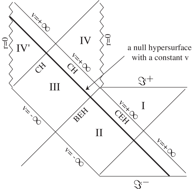
Figure 1: A portion of the conformal diagram for the maximally-extended RNdS solution with three horizons. Zigzag lines represent the timelike central singularities. $\Im^{+(-)}$ corresponds to the future (past) null infinity. The black-hole event horizon (BEH) is the null hypersurface between Regions II and III. The inner horizon as a Cauchy horizon (CH) is that between Regions III and IV or IV^′. The cosmological event horizon (CEH) is that between Regions I and II. Regions I, II, and III correspond to the exterior of the cosmological event horizon, the Region between the black-hole event horizon and the cosmological event horizon, and the Region between the inner horizon and the black-hole event horizon, respectively. Regions IV and IV^′ correspond to the interior of the inner horizon.

We consider static solutions with at least one regular horizon. By the condition of the regularity of horizon, functions $f$, $A$, $\phi$ and $\phi^{\prime}$ and their derivatives with respect to $r$ are finite at the horizon. An example of the spherically symmetric static solution with analytic horizons is the $n$-dimensional RN(A)dS solution, which is given by

$$f=1-\frac{\tilde{M}}{r^{n-3}}+\frac{(n-3)}{2}\frac{\tilde{Q}^{2}}{r^{2n-6}}-\frac{2\Lambda_{\rm eff}}{(n-1)(n-2)}r^{2},$$ (13)

$$\Lambda_{\rm eff}:=\Lambda+\kappa_{n}^{2}V(\phi_{0}),\;\;\;\;A\equiv 0,\;\;\;\;\phi\equiv\phi_{0},$$ (14)

where $\tilde{M}$ and $\tilde{Q}$ are constants related to the mass $M$ and the charge $Q$ of the black hole as

$$\tilde{M}:=\frac{16\pi G_{n}M}{(n-2)\!\Sigma_{n-2}},\;\;\;\;\;\tilde{Q}^{2}:=\frac{\kappa_{n}^{2}Q^{2}}{2(n-2)\pi g_{c}^{2}},$$ (15)

respectively, where $\Sigma_{n-2}$ is the volume of the $(n-2)$-dimensional unit sphere. $\phi_{0}$ is the extremal point of the potential $V$. In this spacetime, the number of horizons varies depending on $\tilde{M}$, $\tilde{Q}$, and $\Lambda_{\rm eff}$ and is always less than or equal to three. The RNdS spacetime with three horizons has, as shown in Fig. 1, a Cauchy horizon, a black-hole event horizon and a cosmological event horizon. There are other known black-hole solutions with analytic horizons, in which the effective cosmological constant $\Lambda_{\rm eff}$ is negative and the first term of the right-hand side in Eq. (13) is replaced by $0$ or $-1$. They are called topological black holes, since the topology of the constant $r$ surface is not $S^{n-2}$. The spacetime structure of these solutions has been investigated Brill ; tm2004 . Spherically symmetric static black-hole solutions with the nontrivial configuration of a scalar field, i.e., a scalar hair, with a double-well potential, has been also found numerically both in four-dimensional asymptotically de Sitter and anti-de Sitter spacetimes, where the former is unstable against spherical perturbations while the latter is stable tmn .

III Kink instability of horizons

We consider full-order radial perturbations $\delta f(v,r),\delta A(v,r)$, and $\delta\phi(v,r)$ in general background static solutions such as

$$f(v,r) = f_{(\rm b)}(r)e^{\delta f(v,r)},$$ (16)

$$A(v,r) = A_{(\rm b)}(r)+\delta A(v,r),$$ (17)

$$\phi(v,r) = \phi_{(\rm b)}(r)+\delta\phi(v,r),$$ (18)

where $f_{(\rm b)},A_{(\rm b)}$, and $\phi_{(\rm b)}$ denote a background static solution that satisfies Eqs. (9)–(12). We consider perturbations that satisfy the following conditions: (i) the initial perturbations only exist inside the horizon, i.e., $r<r_{h}$; (ii) $f$, $A$, $\phi$, and $\phi^{\prime}$ are continuous at the horizon; (iii) $\phi^{\prime\prime}$ and $\dot{\phi}^{\prime\prime}$ are discontinuous at the horizon although they have finite one-sided limit values as $r\to r_{\rm h}-0$ and $r\to r_{\rm h}+0$; (iv) no curvature singularities exist at the horizon at the initial moment.

Now we consider the behavior of perturbations at the horizon. By the condition (i), the region outside the horizon remains unperturbed, i.e., it is described by the background static solution, because no information can propagate beyond the horizon. By condition (ii), $\delta A$, $\delta f$, $\delta\phi$, and $\delta\phi^{\prime}$ vanish at the horizon so that

$$\delta A^{\prime}=0$$ (19)

is satisfied at the horizon from Eq. (10). From Eqs. (11) and (19),

$$\lim_{r\to r_{\rm h}}f_{(\rm b)}\delta f^{\prime}=0$$ (20)

is obtained. Differentiating Eq. (10) with respect to $r$ and evaluating both sides at the horizon, we obtain

$$\frac{n-2}{2r_{\rm h}}\delta A^{\prime\prime}=\kappa^{2}_{n}\phi_{(\rm b)}^{\prime}\delta\phi^{\prime\prime},$$ (21)

which means that $\delta A^{\prime\prime}$ is finite because of condition (iii). Differentiating Eq. (11) with respect to $r$, evaluating both sides at the horizon, and using condition (iii) and Eqs. (19)–(21), we obtain

$$\lim_{r\to r_{\rm h}}[2f_{(\rm b)}^{\prime}\delta f^{\prime}+f_{(\rm b)}(\delta f^{\prime\prime}+\delta f^{{}^{\prime}2})]=0.$$ (22)

Differentiating Eq. (12) with respect to $r$, and using condition (iii) and Eqs. (19)–(22), we find

$$2e^{-A_{(\rm b)}}\delta\dot{\phi}^{\prime\prime}+2f_{(\rm b)}^{\prime}\delta\phi^{\prime\prime}+\lim_{r\to r_{\rm h}}f_{(\rm b)}\delta\phi^{\prime\prime\prime}=0$$ (23)

at the horizon. We can prove the third term on the left-hand side vanishes in the same way as in Appendix B in Ref. hm2004 . As a result, Eq. (23) becomes

$$\delta{\dot{\phi}}^{\prime\prime}=-f_{(\rm b)}^{\prime}e^{A_{(\rm b)}}\delta\phi^{\prime\prime}.$$ (24)

It should be noted that the perturbations are of full-order although this equation is linear. This is integrated to give

$$\delta{\phi}^{\prime\prime}\propto e^{-\alpha v},$$ (25)

where

$$\alpha:=f_{(\rm b)}^{\prime}e^{A_{(\rm b)}}.$$ (26)

Here we define instability by the exponential growth of discontinuity. Then we find the following criterion: anti-transluminal horizons, i.e., horizons with $f^{\prime}>0$, are stable, while transluminal horizons, i.e., horizons with $f^{\prime}<0$, are unstable. Degenerate horizons, i.e., horizons with $f^{\prime}=0$, are marginally stable. Irrespective of the form of the potential $V(\phi)$, this stability criterion applies to any analytical and numerical solutions with regular horizons. In the above, we have discussed the stability of horizons that are future-directed outgoing null geodesics. If horizons are given by future-directed ingoing null geodesics, such as a Cauchy horizon of RN(A)dS solution, we find serious coordinate degeneracy in the $(v,r)$ coordinates. Hence, we need to reformulate the perturbation analysis using the $(u,r)$ coordinates:

$$ds^{2}=-fe^{2A}du^{2}-2e^{A}dudr+r^{2}d\Omega_{n-2}^{2},$$ (27)

where $f=f(u,r)$ and $A=A(u,r)$. $u$ is the retarded time coordinate. Since the above form can be obtained from Eq. (7) through the coordinate transformation $v=-u$, the stability in terms of $u$ should be reversed from that in terms of $v$. Therefore, the stability of horizons which are given by future-directed ingoing null geodesics are the following: anti-transluminal horizons are unstable, while transluminal horizons are stable. Degenerate horizons are marginally stable. In Appendix A, we demonstrate in the four-dimensional spherically symmetric spacetime that these perturbations are gauge-invariant up to linear order.

IV Discussion

We have obtained the stability of horizons in $n$-dimensional static solutions in the Einstein-Maxwell-scalar-$\Lambda$ system without assuming the explicit form of the potential of the scalar field. The RN(A)dS solution is included in the analysis as a special case. The present work has shown for the first time the existence of the kink instability of horizons in static solutions in general relativity. The intriguing feature is that the kink instability grows exponentially in terms of $v$. In contrast the kink mode perturbation blows up to infinity in a finite time in the self-similar perfect-fluid system with $p=k\mu$ ($0<k<1$) in general relativity harada2001 .

The stability of solutions against kink-mode perturbation is determined only by the local property, i.e., the sign of $f^{\prime}$ at the horizon of the background static solutions. This criterion applies to a large class of horizons. For the RNdS spacetime, a black-hole event horizon is stable against the kink-mode perturbation. A cosmological event horizon is also stable. On the other hand, a Cauchy horizon is unstable. As a result, a wide class of solutions suffers from the kink instability. There is a significant difference here from the case of self-similar solutions where the black-hole event horizon is stable but the Cauchy horizon and the cosmological event horizon are not always unstable harada2001 ; hm2004 .

We consider the implications of the kink instability of horizons. The initial perturbations of the kink mode are inserted only in the future of the horizons, and therefore, this instability does $not$ prevent the horizons or the naked singularities from forming. The kink instability implies that, if the analyticity of a horizon is violated even weakly, the perturbed spacetime is much different from that with an analytic horizon. Even so, this kind of instability does not cause the formation of a singularity on the horizon in finite time because the growth of the discontinuity is only exponential.

An important example of kink-unstable horizons is the Cauchy horizon of the RN(A)dS solution, which associates with a timelike naked singularity. It is generated by the first future-directed null ray emanated from the naked singularity. If the naked singularity forms in a gravitational collapse, the information from the singularity, which is physically unpredictable, affects only the future of the Cauchy horizon, and the naked singularity may violate its analyticity. Then, the inside region of the Cauchy horizon is represented by a spacetime much different from that in the RN(A)dS solution.

As a thought experiment, suppose that one drops an ideal small apparatus into the RN(A)dS black hole. In four-dimensional spherically symmetric case, the apparatus never arrives at the regular Cauchy horizon because its back reaction to the spacetime actually disturbs the background before it reaches the Cauchy horizon and the Cauchy horizon is transformed into a null weak curvature singularity pi1990 ; ori1991 ; burko1997 ; burko2003 ; brady1999 ; chambers1997 ; bmm1998 . Here we assume that the ideal apparatus has so small mass that its back reaction to the spacetime can be negligible but can disturb the scalar field at any time. Then, it falls across the event horizon and reaches the Cauchy horizon. At this moment, if it disturbs the scalar field, so that the second derivative of the scalar field is discontinuous, the disturbance grows up through kink instability and propagates along the Cauchy horizon at the speed of light. As a result, the gravitational field inside of the Cauchy horizon is very much modified.

Appendix A gauge-invariance of kink instability

We demonstrate in the four-dimensional spherically symmetric spacetime that the perturbations are gauge-invariant up to linear order. All notations here follow gs . We write the spherically symmetric spacetime as a product manifold ${\cal M}=M^{2}\times S^{2}$ with metric

$$g_{\mu\nu}=\mbox{diag}(g_{AB},r^{2}\gamma_{ab}),$$ (28)

where $g_{AB}$ is an arbitrary Lorentz metric on $M^{2}$, $r$ is a scalar on $M^{2}$ with $r=0$ defining the boundary of $M^{2}$, and $\gamma_{ab}$ is the unit curvature metric on $S^{2}$. We introduce the covariant derivatives on spacetime ${\cal M}$, the subspacetime $M^{2}$ and the unit sphere $S^{2}$ with

$$g_{\mu\nu;\lambda} = 0,$$ (29)

$$g_{AB|C} = 0,$$ (30)

$$g_{ab:c} = 0.$$ (31)

We denote a perturbed scalar field $\phi$ as

$$\phi=\phi_{(\rm b)}+\delta\phi.$$ (32)

Hereafter we linearize the perturbation.

The perturbation of the scalar field is transformed by a gauge transformation of even parity as

$$\delta{\bar{\phi}}=\delta\phi-\phi_{{(\rm b)};\mu}\xi^{\mu},$$ (33)

where $\xi^{\mu}$ is a generator of the infinitesimal coordinate transformation.

Spherically symmetric metric perturbations are written as

$$\delta g_{AB} = h_{AB}Y,$$ (34)

$$\delta g_{ab} = r^{2}KY\gamma_{ab},$$ (35)

where $h_{AB}$ and $K$ are a tensor and a scalar on $M^{2}$ and $Y$ is a constant. For spherical perturbations, all gauge transformations we have for metric perturbations are

$${\bar{h}}_{AB} = h_{AB}-(\xi_{A|B}+\xi_{B|A}),$$ (36)

$${\bar{K}} = K-2v_{A}\xi^{A},$$ (37)

where $v_{A}:=r_{,A}/r$. Here, for simplicity, we have chosen the areal coordinate $r$ as a radial coordinate, i.e., $x^{1}=r$, for the background spacetime.

Since

$$v_{A}=\frac{r_{|A}}{r}=\left(0,\frac{1}{r}\right),$$ (38)

we have

$$\xi^{1}=-\frac{r}{2}({\bar{K}}-K),$$ (39)

from Eq. (37). Using the fact that $\phi_{(\rm b)}$ depends only on $r$, we can construct the following gauge invariant perturbation $\Phi$:

$$\Phi=\delta\phi-\frac{r}{2}K\frac{d\phi_{(\rm b)}}{dr}.$$ (40)

When we choose the areal coordinate $r$ as a radial coordinate in the perturbed spacetime, which is adopted in the main text of the present article, $K=0$ is satisfied so that the gauge invariant quantity $\Phi$ is identical to $\delta\phi$ in this gauge choice. For the gradient and higher derivatives of the scalar field, we can construct them just by covariantly differentiating $\Phi$ on the background metrics.

References

- (1) S. Chandrasekhar, The Mathematical Theory of Black Holes (Oxford University Press, New York, 1992).
- (2) S.W. Hawking and G.F.R. Ellis, “The Large Scale Structure of Space-time” (Cambridge University Press, Cambridge, England, 1973).
- (3) R. Penrose, Riv. Nuovo Cim.1, 252 (1969).
- (4) R. Penrose, in General Relativity, an Einstein Centenary Survey, edited by S.W. Hawking and W. Israel (Cambridge University Press, Cambridge, England, 1979), p. 581.
- (5) R. Penrose, in Battelle Rencontres, edited by C. de Witt and J.A. Wheeler (W.A. Benjamin, New York, 1968), p. 222.
- (6) E. Poisson and W. Israel, Phys. Rev. D41, 1796 (1990).
- (7) P.R. Brady, Prog. Theor. Phys. Suppl. 136, 29 (1999).
- (8) A. Ori, Phys. Rev. Lett.67, 789 (1991).
- (9) L.M. Burko, Phys. Rev. Lett.79, 4958 (1997).
- (10) L.M. Burko, Phys. Rev. Lett.90, 121101 (2003); Erratum, ibid 90, 249902(E) (2003).
- (11) C.M. Chambers, in Internal Structure of Black Holes and Spacetime Singularities: Proceedings (Annuals of the Israel Physical Society Series, No 13), edited by L.M. Burko and A. Ori (Institute of Physics Publishing, Bristol, England, 1998), p. 33, e-print gr-qc/9709025.
- (12) P.R. Brady, I.G. Moss, and R.C. Myers, Phys. Rev. Lett. 80, 3432 (1998).
- (13) T. Harada, Pramana 63, 741 (2004), as Proceedings of the 5th International Conference on Gravitation and Cosmology, Jan 5-10, 2004, Cochin, India.
- (14) P. Kraus, J. High Energy Phys. 12, 011 (1999); D. Ida, J. High Energy Phys. 09, 014 (2000).
- (15) A. Ori and T. Piran Mon. Not. R. Astron. Soc. 234, 821 (1988).
- (16) T. Hanawa and T. Matsumoto, Publ. Astron. Japan 52, 241 (2000).
- (17) T. Harada, Class. Quantum Grav. 18 4549 (2001).
- (18) T. Harada and H. Maeda, Class. Quantum Grav. 21, 371 (2004).
- (19) H. Maeda and T. Harada, Phys. Lett. B, in press, gr-qc/0412040.
- (20) S. Kato, F. Honma, and R. Matsumoto, Mon. Not. R. Astron. Soc. 231 37 (1988); S. Kato, W. Xue-bing, Y. Lan-tian, and Y. Zhi-liang, ibid 260 317, (1993); B. Muchotrzeb-Czerny, Acta Astron., 36 1, (1986).
- (21) D.R. Brill, J. Louko, and P. Peldan, Phys. Rev. D56, 3600 (1997).
- (22) T. Torii and H. Maeda, in preparation.
- (23) T. Torii, K. Maeda, and M. Narita, Phys. Rev. D59, 064027 (1999); ibid 59, 104002 (1999); ibid 63, 047502 (2001); ibid 64, 044007 (2001).
- (24) U.H. Gerlach and U.K. Sengupta, Phys. Rev. D 19, 2268 (1979); ibid 22, 1300 (1980).