Cosmic string scaling in flat space

Abstract

We investigate the evolution of infinite strings as a part of a complete cosmic string network in flat space. We perform a simulation of the network which uses functional forms for the string position and thus is exact to the limits of computer arithmetic. Our results confirm that the wiggles on the strings obey a scaling law described by universal power spectrum. The average distance between long strings also scales accurately with the time. These results suggest that small-scale structure will also scale in expanding universe, even in the absence of gravitational damping.

I Introduction

During phase transitions in the early universe various topological defects can form. In particular, cosmic string networks are formed when symmetry is broken and the vacuum manifold contains incontractible loops Kibble . Fundamental or $D$-strings formed at the end of brane inflation can also play the role of cosmic strings Tye ; Polchinski ; Gia . Primordial string networks can produce a variety of observational effects: linear discontinuities in the microwave background radiation, gravitational lensing, gamma ray bursts, and gravitational radiation — both bursts and a stochastic background (for a review of cosmic strings, see VS ; KH ).

An evolving string network consists of two components: long strings and sub-horizon closed loops. The long string component is characterized by the following parameters: the coherence length $\xi(t)$, defined as the distance beyond which the directions along the string are uncorrelated, the average distance between the strings $d(t)$, and the characteristic wavelength of the smallest wiggles on long strings, $l_{min}(t)$. The standard picture of cosmic string evolution assumes that all three of these scales grow proportionately to the horizon size $t$ and that the typical size of loops is set by $l_{min}(t)$.

Previous simulations of strings in an expanding universe Bennett ; Shellard have only partially confirmed this model. The long strings were observed to scale with

$$\xi(t)\sim d(t)\propto t,$$ (1)

but the short wavelength cutoff $l_{min}$ and the loop sizes did not scale, remaining at the resolution of the simulations. It is not clear whether this is a genuine feature of string evolution or a numerical artifact. A flat-space simulation introduced in Smith and further developed in Maria and Hindmarsh had the same problem. Moreover, the rate of growth of $\xi(t)$ and $d(t)$ in that simulation showed dependence on the lower cutoff imposed on loop sizes, indicating that lack of resolution at small scales can affect long string properties.

It is generally believed that in a realistic network the scaling behavior of the cutoff scale $l_{min}(t)$ will eventually be enforced by the gravitational back-reaction. However, it has been recently realized that this back-reaction is much less efficient than originally thought OS and that the cutoff scale is sensitively dependent on the spectrum of small-scale wiggles OSV . Thus, it becomes important to determine the form of the spectrum.

Here we have developed an algorithm and have performed a cosmic string network simulation that lacks the problem of smallest resolution scale. Rather than representing the string as a series of points which approximate its position, we use a functional description of the position which can be maintained exactly (except for the inevitable inaccuracy of computer arithmetic) in flat space. After the simulation has run for some time and the total length of string has decreased, we expand the simulation volume, as discussed below. This technique enables us to reach an effective box size greater than 1000 times the initial correlation length. Such a technique could also be used in expanding-universe simulations.

The results of the simulation will be discussed in a series of publications. In the current paper we present the algorithm of our simulation and concentrate on the evolution of infinite strings, focusing in particular on the spectrum of small-scale wiggles. In section II we describe the algorithm of our simulation and its complexity, in section III we show that the spectrum of small wiggles exhibits scaling behavior. In section IV we analyze the behavior of the inter-string distance and correlation length, and show that they scale with the time. In section V we discuss what can be learned about the expanding universe from this flat-space simulation.

II Numerical Simulation

II.1 Algorithm

The evolution of a cosmic string with thickness much smaller than radius of its curvature can be described by the Nambu action. In general, the equations of motion of cosmic strings cannot be solved analytically. However, in flat space-time they are greatly simplified (see VS ; KH for detailed discussion). The Nambu action is invariant under arbitrary reparametrization of the two-dimensional worldsheet swept by the string. We take the time $t$ as one parameter and a spacelike parameter $\sigma$ giving the position on the string. With the usual parameter choice, the string trajectory $\mathbf{x}(t,\sigma)$ obeys

$$\mathbf{\dot{x}}\cdot\mathbf{x}^{\prime} = 0,$$ (2)

$$\dot{\mathbf{x}}^{2}+\mathbf{x}^{\prime 2} = 1,$$ (3)

with the equation of motion

$$\ddot{\mathbf{x}}-\mathbf{x}^{\prime\prime}=0,$$ (4)

where prime denotes differentiation with respect to $\sigma$ and dot differentiation with respect to $t$.

The general solution to these equations can be described by separating left- and right-moving waves:

$$\mathbf{x}(t,\sigma)=\frac{1}{2}\left(\mathbf{a}(\sigma-t)+\mathbf{b}(\sigma+t)\right),$$ (5)

with

$$\mathbf{a}^{\prime 2}=\mathbf{b}^{\prime 2}=1.$$ (6)

With this solution in hand we can follow the evolution of each string in the network exactly. Having computed $\mathbf{a}$ and $\mathbf{b}$ from the initial conditions we can find the position of each string at any later time $t$.

When their trajectories intersect, strings can exchange partners with some probability $p$. For gauge theory strings, $p$ is essentially 1, but fundamental strings and 1-dimensional D-branes can have substantially lower $p$. In the present analysis we are concerned only with $p=1$. Smaller $p$ will be the subject of a future paper.

Such an intercommutation introduces discontinuities (kinks) in the functional forms of the $\mathbf{a}$ and $\mathbf{b}$ describing the strings. We update the form accordingly and once again string positions can be computed exactly. This procedure was used by Scherrer and Press SP and Casper and Allen CA to simulate the evolution of a single loop; here we use it for a network.

In the expanding universe, small loops which are produced at intercommutations will almost never encounter another string and so will not rejoin to the network. To capture this feature in a flat-space simulation, we explicitly disallow loops of length $l<\kappa t$ to rejoin the network, as was done in Maria ; Hindmarsh . Here, $\kappa$ is a constant (typically taken as 0.25) and $t$ is the time which has so far been simulated. Of course the results of such a technique can be trusted only if they are not sensitive to the particular choice of $k$, and that expectation is confirmed below.

To generate initial conditions we use the Vachaspati-Vilenkin prescription 6 in a periodic box of size $L$, usually 100 in units of the initial correlation length. Where the string produced by that technique crosses straight through a cell we use a straight segment and where it enters a cell and exits through an adjacent face we use a quarter circle. However, to simplify the implementation we replace the quarter circle with $K$ straight segments (connecting points lying on the quarter circle). In the present paper we use $K=2$. We expect our results to be insensitive to the choice of $K$, and in fact tests with $K=4$ showed no significant difference.

An initially static string of length $l$ will collapse into a double loop at time $t=l/4$ KT . To prevent such a collapse we perturb the initial conditions by giving small initial velocities to the part of the string inside each cell in the normal direction to the local plane of the string.

II.2 Implementation

To represent the piecewise linear form of $\mathbf{a}$ and $\mathbf{b}$ we store the constant values of $\mathbf{a}^{\prime}$ and $\mathbf{b}^{\prime}$ for each segment, together with values for $\mathbf{a}(0)$ and $\mathbf{b}(0)$. To perform an intercommutation we introduce 2 points for each of $\mathbf{a}^{\prime}$ and $\mathbf{b}^{\prime}$ and then concatenate or split the lists of $\mathbf{a}^{\prime}$ and $\mathbf{b}^{\prime}$ depending on whether two strings are joining into one or one string is splitting in two.

The world sheet of the piecewise linear string consists of flat pieces that we call diamonds glued together along four lines each, two constant values of $a(\sigma-t)$ and two constant values of $b(\sigma+t)$. Each diamond has some extent in space and time. At any moment, we have a list of all diamonds that intersect the current time. With each diamond we store the spacetime position of the corners, so that we don’t have to integrate $\mathbf{a}^{\prime}$ and $\mathbf{b}^{\prime}$ to find the string position.

When the current time exceeds the ending time of some diamond we discard that diamond and generate a new one in the future light-cone of the old one with the starting time of the new diamond equal to the ending time of the discarded diamond. When each new diamond is generated, we check it for intersections with every existing diamond. To accomplish this in unit time, we divide the entire simulation box into small boxes a little bit larger than the largest extent of any single diamond. With each box we store a list of diamonds that intersect it. Each diamond can intersect at most 7 boxes. When the diamond is created we check each box that it intersects for possible intercommutations.

This algorithm does not necessarily generate intercommutations in causal order, so when we detect one we store its parameters in a time-ordered list of pending intercommutations. When the current time reaches the time of a pending intercommutation, the intercommutation is then performed. If instead we find an intercommutation in the backward light cone of a pending one, we invalidate the pending one when the earlier one is performed.

To be able to quickly determine the length of a newly created loop, we store the $\mathbf{a}^{\prime}$ and $\mathbf{b}^{\prime}$ values in a “skip list” 7 , which permits integration of the displacements in $\sigma$ and updating for intercommutations, both in time proportional to $\log l$.

The complexity of the above algorithm can be calculated in the following matter. In a box of size $L$ in units of initial correlation length, $L^{3}$ random phases are generated. There are $3L^{3}$ edges and each of them has a probability of 8/27 to have a string. On average we have $(8/9)L^{3}$ of total string length in the box of volume $L^{3}$. Most of the string length is in a single long string which is constantly intercommuting with itself and with other loops. To store $\mathbf{a}^{\prime}$ and $\mathbf{b}^{\prime}$ for all strings in the network, we need on average $2(8/9)L^{3}K$ data points and about the same number of diamonds. Thus the memory usage scales as $L^{3}K$.

We use a “calendar queue” 8 to store the list of diamonds, which allows us to find the diamond with the earliest ending time and to insert a new diamond into the list, both in constant CPU time. Thus the entire procedure of finding the oldest diamond, removing it, replacing it with a new diamond, and checking that diamond for intercommutations requires only a constant amount of CPU time. When an intercommutation takes place, the runtime is proportional to the logarithm of the length of the strings involved, because of the skip list, but intercommutations are sufficiently rare that the time spent searching for intercommutations dominates over the time spent performing them.

The lifetime of a diamond depends on the lengths of the segments on its edges, which are typically $1/K$. Thus every time $1/K$ we need to process of order $L^{3}K$ diamonds. We typically simulate the network for cosmic time of the order of the light crossing time of the box $L$. Therefore the final overall running time of the program scales as $L^{4}K^{2}$.

Tufts has a Linux computation cluster on which we performed our simulations. Each of 32 nodes has a dual 2.8 GHz CPU and 3 GBytes of usable memory. Each run of the simulation runs on a single node. The memory constrains the box size to about 100 in initial correlation length, and it takes about 5 hours to evolve the network for one light crossing time of such a box. The existence of multiple nodes allows 32 simulations to be run simultaneously, so that we can do about 150 runs in a day.

The code is written entirely in ANSI C, so it is easily portable across different platforms. It was successfully tested and ran on Windows and Linux PCs.

II.3 Expansion of the box

In the previous section we have pointed out that the boundary effects become important when the cosmic time of the simulation is of order $L$. To avoid problems that have nothing to do with physics of the process, we would like all of the length scales of the network to be much smaller than the size of the box. In the discussion below, we propose a technique that allows us to overcome boundary effects and push the effective box size and thus the running time of the simulation to larger values.

Since small loops smaller than a threshold are not allowed to rejoin the network, we can remove them from the simulation when they are produced, and so decrease the the total string length. The computer memory used by simulation is proportional to the total string length divided by the average size of the segments. Each intercommutation introduces four kinks and thus decreases the average size of the segments. This process increases the memory used by simulation by a small constant amount. On the other hand when string loops decouple from the simulation the memory is freed on average by the amount proportional to their length. In the following discussion we shall assume that the memory usage of the simulation is proportional to the string length only, since we found that the decrease of the segment size gives only a small correction to the calculations and does not change the general idea.

Suppose that the string network is in the scaling regime. If so, the inter-string distance grows linearly with $t$, and thus the total string length in long strings decays as $t^{-2}$. Therefore, by some time $t_{1}$, when the string length has decreased by a factor of 8, the inter-string distance has grown by a factor of $\sqrt{8}$. If we are only interested in behavior of infinite strings we can expand the box at time $t_{1}$ from initial size $L^{3}$ to $(2L)^{3}$ and continue the evolution further.

The simplest way to expand the box it to create 8 identical replicas of the box of size $L^{3}$ at time $t_{1}$ and to glue them together to form a box of size $(2L)^{3}$. This introduces correlations on the super horizon distances that we should disturb by some mechanism to avoid similar evolution of 8 boxes. If we do not do anything and continue the evolution the result will not be different from evolution of a single box where boundary effects become important at some time of order $L$.

There are several ways that one can think of to disturb the periodicity. The most promising approach that we have found, that does least violence to the network is the following. Right after the expansion we change the intercommutation probability to p=0.5 for some fraction of the elapsed time and then change intercommutation probability back to p=1. The time during which we force the intercommutation probability to be a half should be at least the inter-string distance in order to introduce enough entropy into the system. The hope is that after $p=1$ is switched back on the system will quickly return to the properties appropriate to $p=1$

By the described procedure the expansion takes place roughly when the total string length in long strings has decreased by 8. The average time of expansions is the same regardless of the initial box size $L$, so if we choose $L>t_{1}$ the first expansion would take place before the boundary effects become important. However, the effective box size grows in steps given by a power law $t^{2/3}$, and therefore regardless of initial $L$ the effective box size would eventually become smaller than current time. In order to be able to run the simulation longer we have to be able to expand the box sooner. In fact if we could have expanded the box when the total length in long strings has decreased by 4, the effective box size would grow linearly with time. This can be achieved if we also modify the string at the time of expansion by removing half of the points of long strings to increase the average size of the segments by two.

Each string consists of about the same number of left and right moving kinks, and our job is to replace it with half as many points that represent a smoothed version of the original string. One possibility is to remove three out of every four kinks (both left and right moving) and connect the remaining points with straight segments. Then each of the remaining points is decomposed into two kinks, one left and one right moving. At this point we still have a freedom to give new segments any velocities we like in the direction orthogonal to the tangent vector of the string. To set each new segments with new velocities we find an average velocity of old four segments and project it to the transverse plane of the new segment. This algorithm shortens the string length since we replace four consecutive segments with a single straight segment. Although the inter-string distance defined as a $1/\sqrt{\rho}$ becomes larger after smoothing, the real inter-string distance, that describes the average distance between nearby long strings, does not change.

The expansion of the box technique with smoothing can be carried on over and over again until we run into another problem of periodic boundary conditions, but the effective box size would be somewhat larger. The new problem has to do with the fact that overall linkage of the initial box is zero. However, we would like to think of our box as a small part of an infinite space. This means that the overall linkage of the box should be some random number with distribution peaked around zero, but not identically zero. On the other hand, the zero linkage of the box results in very odd configurations of the network at late times: for any long string with linkage in, say, the positive $x$ direction, there must be another string close by linked in the negative $x$ direction. This effect leads to overproduction of small loops, because the configuration is not stable and long strings would tend to unlink themselves. It prevents us from expanding the box indefinitely.

III Scaling Properties

We will primarily be concerned with the amplitude of small wiggles on infinite strings. To have a time-independent description of these wiggles, we will consider wiggles in the functions $\mathbf{a}$ and $\mathbf{b}$. With a very long loop of string, we can define a Fourier transform of the tangent vector,

$$\mathbf{A}(k)=\frac{1}{\sqrt{2\pi l}}\int_{0}^{l}d\sigma\,\mathbf{a}^{\prime}(\sigma)e^{-ik\sigma}$$ (7)

where $l$ is the loop length, and $k=k_{n}=2\pi n/l$ for $n$ an integer. We will work in the limit where $l\to\infty$, so that $k$ becomes a continuous variable, but because our functions do not fall off at large $\sigma$, we will have to retain the parameter $l$.

There will be some level of correlation between different modes. For example, since modes of similar size can collectively form a loop we would expect a large mode which had survived on a long string to be accompanied by smaller than average modes of similar wavenumber. Nevertheless, we can get some idea of the string shape by ignoring such correlations and taking

$$\langle\mathbf{A}(k)\cdot\mathbf{A}^{*}(k^{\prime})\rangle=\begin{cases}c(k)&k=k^{\prime}\\ 0&k\neq k^{\prime}\end{cases}$$ (8)

where the averaging is over realizations of the string network. Because of the factor $1/\sqrt{l}$ in Eq. (7), $c(k)$ does not depend on $l$,

$$c(k)=\frac{1}{2\pi}\int_{0}^{l}d\sigma e^{ik\sigma}C(\sigma),$$ (9)

where $C(\sigma)$ is the correlation function

$$C(\sigma)=\langle\mathbf{a}^{\prime}(0)\mathbf{a}^{\prime}(\sigma)\rangle.$$ (10)

The values $\mathbf{A}(k)$ for different $k$ have no correlation. In the limit $l\to\infty$, these different points become arbitrary close, so $\mathbf{A}(k)$ is everywhere discontinuous. However, $c(k)$ is a continuous function, and $c(-k)=c(k)$ since $C(\sigma)$ is real.

The inverse transformation to (7) is

$$\mathbf{a}^{\prime}(\sigma)=\sqrt{\frac{2\pi}{l}}\sum_{n=-\infty}^{\infty}e^{ik_{n}\sigma}\mathbf{A}(k_{n})$$ (11)

From Eqs. (6) and (8),

$$1=\langle\mathbf{a}^{\prime}(\sigma)^{2}\rangle=\frac{2\pi}{l}\sum_{n=-\infty}^{\infty}c(k_{n})\approx\int_{-\infty}^{\infty}dk\,c(k)$$ (12)

Similar relations apply for $\mathbf{b}^{\prime}(\sigma)$.

We can define a “spectral power density”,

$$P(k)=2kc(k)$$ (13)

so that

$$\int_{0}^{\infty}P(k)\,d\ln k=1\,.$$ (14)

The quantity $P(k)$ is the fractional contribution to the energy density of the string from modes in a logarithmic interval around $k$.

For Vachaspati-Vilenkin initial conditions it has been shown that properties of long strings are similar to properties of a random walk 6 . Computing the power spectrum for a random walk of step size $h$ gives

$$P(k)=\frac{4}{\pi kh}\sin^{2}(kh/2)\to\begin{cases}kh/2&kh\ll 1\\ 2/(\pi kh)\text{ on average}&kh\ll 1\end{cases}$$ (15)

We create our initial conditions with straight segments of length 1 and piecewise linear approximations to curved segments of length $\pi/4$. However, we have some correlation between successive segments, so the effective correlation length of the random walk in the initial conditions is $h\approx 1.62$ as shown in Fig. 1.

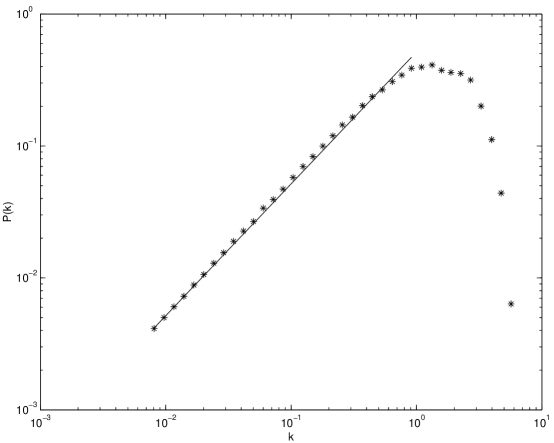
Figure 1: Initial power spectrum. The spectrum at large scales is well fit by the random walk spectrum with step size $h=1.62$.

We do not attempt here to fit the small-scale power spectrum, which depends on the detailed choice of the piecewise linear string.

How should the structures on a string evolve at late times? If there is a scaling regime, and if a certain fraction of the power is between wave numbers $k$ and $k^{\prime}$ at time $t$, then the same fraction of the power will be found between wavenumbers $k/\lambda$ and $k^{\prime}/\lambda$ at time $\lambda t$. This implies that $P(k)$ is a function of $kt$ alone.

Any function $P(kt)$ would give scaling, but we can make some guesses about the shape of this function. First of all, on scales larger than horizon (i.e., $kt\gg 1$), we have a random walk, so $P(kt)\propto kt$. The function $P(k)$ outside the horizon is increasing with time, but that is just a result of the smoothing of the string on smaller scales and our definition of the power.

Inside the horizon, we expect loop production to smooth the string. If there are large excursions in $\mathbf{a}$ and $\mathbf{b}$ at any scale, we expect them eventually to overlap with each other in such a way as to intercommute and produce a loop. The loop will then be removed from the string and the power at that scale will decrease because it has gone into the loop. The typical angle that such excursions make with the general direction of the string is given by an integral of $P(k)$ over a range of wavenumbers describing the size of the wiggle. We thus expect that this process will reduce $P(k)$ below some critical value independent of $k$, at which the wiggles are large enough to produce loops.

If that were the only smoothing process, we would expect a constant spectrum $P(kt)$. But even very small-amplitude structure can be smoothed by other processes, such as loop emission at cusps. If the large-scale structure would produce a cusp, then small wiggles can produce instead a self-intersection that emits a loop. The process is similar to the emission of vortons at cusps vortongun . If a region of string has particularly large wiggles, it is more likely to be emitted into a loop by this process, so there will be gradual smoothing even on scales that are already quite smooth. Thus we might expect some decline below the flat spectrum.

In Fig. 2,

Figure 2: The network of long strings at time 100 of a simulation run in a box of size 100 in units of initial correlation length.

we show a picture of the network of long strings at the end of a run without expansion of the box technique, and in Fig. 3,

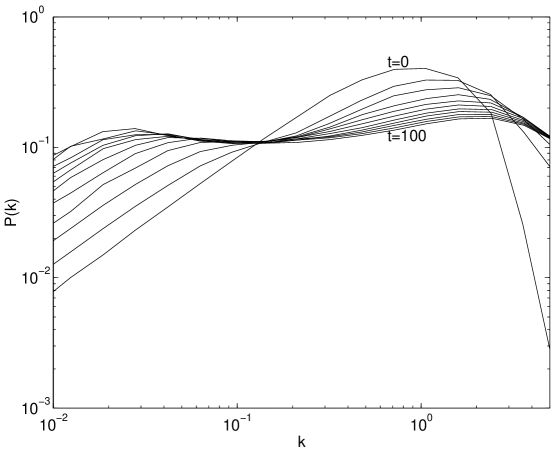
Figure 3: Evolution of the power spectrum from the initial conditions in steps of 10 to $t=100$ in a box of size 100.

we see the power spectrum at different times. The production of small loops constantly reduces the power on the scale of the initial correlation length.

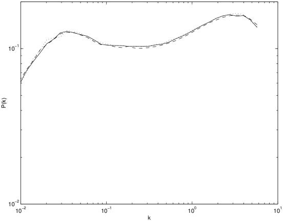
Figure 4: Final power spectrum for rejoin cutoff constant $\kappa=0.125$ (dashed), 0.25 (solid), and 0.5 (dotted).

In Fig. 4, we compare the power spectra at $t=100$ for various values of the cutoff $\kappa$ which controls how small a loop is allowed to rejoin the network. We see that the choice of this cutoff has little effect on the results. In fact, even allowing all rejoining has a fairly minor effect.

In Fig. 5,

Figure 5: Part of the network of long strings at time 960 after 4 doublings of the box size.

we see a picture of the network of long strings at time 960, after 4 doublings of the box size, and in Fig. 6,

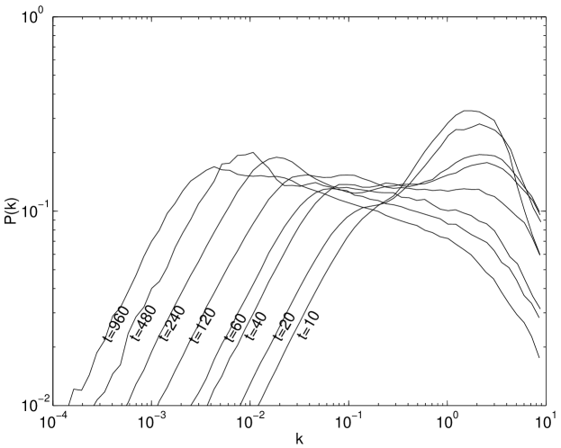
Figure 6: Evolution of the power spectrum vs. $k$ at late times with expansion of the box technique

we plot the evolution of the power spectrum. We also show the evolution of power spectrum vs. $kt$ in Fig. 7,

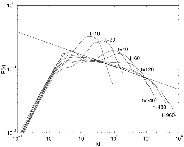
Figure 7: Evolution of the power spectrum vs. $kt$ at late times with expansion of the box technique

to demonstrate that all spectral lines cluster along some universal power spectrum. This demonstrates that the power spectrum at late times is a function of $kt$ alone, just like we would expect for a scaling network. The slowly declining part of the spectrum has a small power law dependence, which is presumably a result of processes such as loop emission near cusps. The best fit power law is

$$P(kt)=0.25(kt)^{-0.18}\,,$$ (16)

only a small correction to the flat spectrum.

We cannot see this power law extend to arbitrarily large $kt$, since we are smoothing the string at small scales as part of the expansion procedure. But we conjecture that without this smoothing we would find the form shown in Fig. 7 with the power law decline eventually extending to arbitrarily large $kt$. In that case, at late times the power spectrum will fall off smoothly to very low levels, rather then coming to a sudden end at some scale $l_{min}$. Because the exponent in Eq. (16) is negative there will be no small-scale divergence in the integral in Eq. (14).

IV Length Scales

From the discussion above we expect structures on each string to scale, and we also expect that the properties of the network as a whole should exhibit scaling. Thus any characteristic length must be proportional to the time $t$.

We will consider two such lengths. The first is the average distance between strings, which we define in a simple fashion ACK

$$d(t)=\sqrt{1/\rho}\,.$$ (17)

where $\rho$ is the length of infinite strings per unit volume. In the case of our simulation box of size $L$,

$$d(t)=\sqrt{L^{3}/{\cal L}(t)},$$ (18)

where ${\cal L}(t)$ is the total string length of long strings. To compute $d(t)$, we have to specify which strings are “long”, but fortunately the result is insensitive to the exact definition. The result for length cutoff $0.25t$ is shown in Fig. 8.

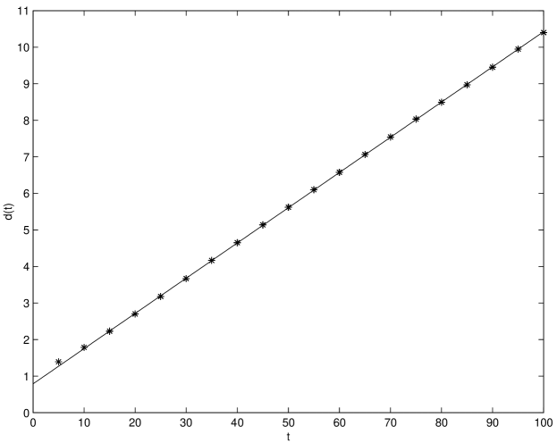
Figure 8: Inter-string distance $d(t)$ at various times (points). The line is $d(t)=0.096(t+8.2)$.

The distance is a linear function of $t$, but the $t$-intercept is not at $t=0$. Instead the best fit line is

$$d(t)=0.096(t+8.2)\,.$$ (19)

Thus it appears that, at late times, the typical string distance is only about 1/10 of the elapsed time since the start of the simulation (here called $t=0$). Since our initial conditions had inter-string distance about 1, they correspond to an initial setting of the natural time parameter about 10.

In Fig. 9,

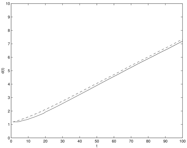
Figure 9: Average distance between long strings $d(t)$ computed by considering long strings to be those longer than $0.25t$ (solid), $1.0t$ (dotted) and $5.0$ (dashed).

we show the inter-string distance computed for various values of the threshold used to define “long” strings. We see that changing this parameter has little effect on the distance computation.

With expansion of the box we can run for much longer. Fig. 10

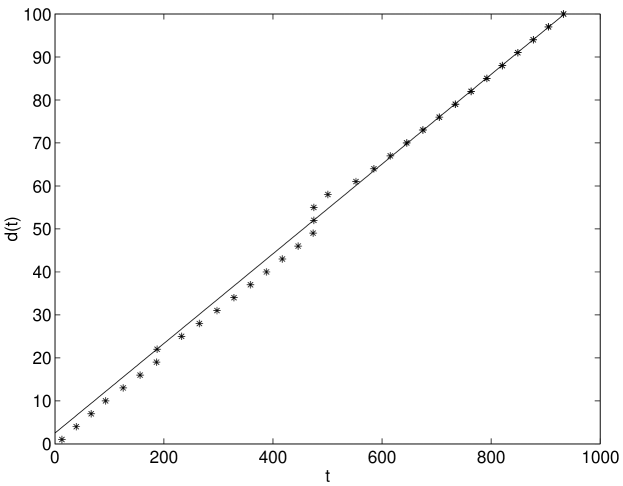
Figure 10: Inter-string distance $d(t)$ with expansion of the box.

shows the inter-string distance out to time 1000. The evolution remains linear, but there is a jump each time the box is expanded.

The second scale is a correlation length $\xi(t)$, such that the tangent vectors to the string at two points separated by distance $\xi(t)$ still have significant correlation. To minimize the dependence of this measure on structure at very small scales, we proceed as follows. Let $\mathbf{r}(\sigma,l)$ be the integral of the tangent vector $\mathbf{a}^{\prime}$ between $\sigma$ and $\sigma+l$, or equivalently the total displacement in $\mathbf{a}$ between those points,

$$\mathbf{r}(\sigma,l)=\mathbf{a}(\sigma)-\mathbf{a}(\sigma+l)$$ (20)

One can use $\mathbf{b}$ in precisely the same way. A measure of the correlation at separation $l$ is given by the dot product between successive segments,

$$C(l)=\langle\hat{\mathbf{r}}(\sigma,l)\cdot\hat{\mathbf{r}}(\sigma+l,l)\rangle$$ (21)

where $\hat{\mathbf{r}}=\mathbf{r}/|\mathbf{r}|$. The average physical separation between points on scales $l$ is given by

$$r(l)=\langle|\mathbf{r}(\sigma,l)|\rangle\,.$$ (22)

We define the correlation length $\xi(t)$ to be $r(l)$ at the scale where $C(l)=0.2$. The choice of the relatively small value 0.2 is motivated by attempting to reduce the contribution of small scales as much as possible while still having a threshold that one can clearly distinguish from no correlation.

In Fig. 11 we show the linear growth of $\xi(t)$. The best-fit straight line is

$$\xi(t)\sim 0.41t\,.$$ (23)

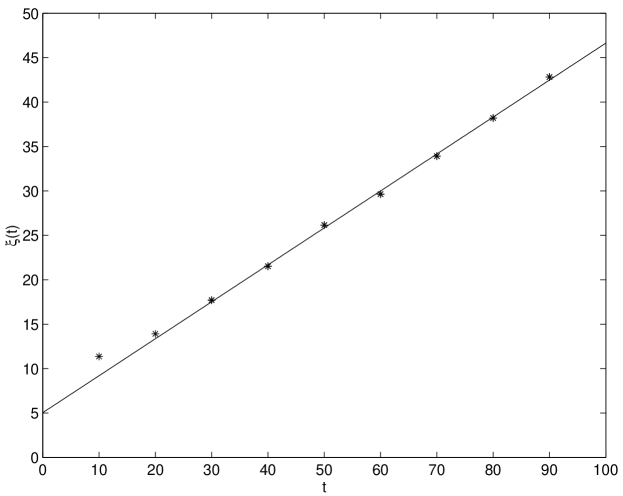
Figure 11: Correlation length $\xi(t)$. The evolution is very nearly linear with $\xi(t)\sim 0.41t$.

The same quantity is plotted in Fig. 12 with box expansion.

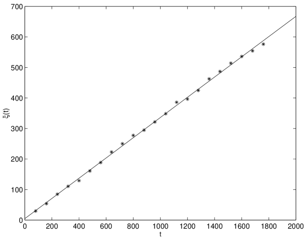
Figure 12: Correlation length $\xi(t)$ with expansion of the box technique. The best-fit straight line is $\xi(t)\sim 0.34t$

A different correlation length scale was defined by Austin, Copeland, and Kibble ACK , who used

$$\bar{\xi}=\int_{0}^{\infty}d\sigma\,C(\sigma)$$ (24)

The scale behaves similarly to $\xi(t)$ in our simulation, except that there are significant jumps at each expansion because smoothing eliminates the small-scale structure.

One way to interpret this situation is to take the part of the run before the final expansion as preparation of initial conditions for the part that comes afterward. Our initial configuration was not very close to the configuration of the scaling network because there is too much structure at the initial correlation length. After the last expansion if our choice of the initial condition matches the one of the scaling network we would get into the scaling regime fast enough before running into the problem of finite box size. With this interpretation we would not have to worry too much about jumps in $d(t)$ (or in $\xi(t)$, although the definition above mostly eliminates those).

V Discussion

Given our results for flat space, what can we say about the situation in an expanding universe? We might hope that our results could be taken over into an expanding space-time with our spatial and temporal coordinates becoming conformal distances and comoving time, but there is potentially an important difference because the expansion of the universe can damp the oscillating wiggles.

A simple model OSV would be to imagine that intercommutations act at the horizon scale to produce a spectrum in which $P$ depends only on $kt$ as we found above. A mode thus enters the horizon with $P(kt)=P$ when $k\sim 1/t$, where $t$ is the conformal time. Assuming that the mode is not affected by larger-wavelength modes that are being damped as in 9 , its comoving $k$ is unchanged. Comoving mode amplitudes, however, decrease with the increase of the scale factor, so we find the amplitude goes as

$$\frac{a_{k}}{a_{0}}=\left(\frac{t_{k}}{t_{0}}\right)^{\alpha}\sim\frac{1}{(kt_{0})^{\alpha}}$$ (25)

where $t_{k}$ is the time where the mode entered the horizon, $a_{k}$ is the scale factor at that time, $t_{0}$ and $a_{0}$ are the present time and scale factor, and the exponent $\alpha$ gives the dependence of scale factor on time, $a(t)\sim t^{\alpha}$ with $\alpha=1$ in the radiation-dominated universe and $\alpha=2$ in the matter-dominated universe. The amplitude appears squared in $P(k)$, so in this model we would find $P(k)\sim k^{-2}$ for radiation dominated and $k^{-4}$ for matter dominated.

This model is overly simplistic, and in reality the interactions between intercommutations and expansion are more complex. Nevertheless we expect that expansion can only make the string smoother than in the flat-space case, so there will be a scaling solution in the expanding universe, even without gravitational damping. We expect the spectrum to have a power law form with exponent between the values above and the flat space result given by Eq. (16).

In upcoming publications we will discuss the questions of loop production and fragmentation, the average velocity and effective mass density of long strings, and the evolution of strings with different intercommutation probabilities $p<1$.

References

- (1) T.W.B. Kibble, J. Phys. A9, 1387 (1976)
- (2) S. Sarangi and S.H. Tye, Phys. Lett. B536, 185 (2002); N. Jones, H. Stoica and S.H. Tye, JHEP 01, 036 (2002)
- (3) E.J. Copeland, R.C. Myers and J. Polchinski, JHEP 06, 013 (2004)
- (4) G. Dvali and A. Vilenkin, JCAP 0403, 010 (2004)
- (5) A.Vilenkin and E.P.S. Shellard, Cosmic Strings and Other Topological Defects (Cambridge, U.K.: Cambridge University Press, 2000).
- (6) M.B. Hindmarsh and T.W.B. Kibble, Rept. Prog. Phys. 58, 477 (1995)
- (7) D.P. Bennett and F.R. Bouchet, Phys. Rev. D41, 2408 (1990)
- (8) B.Allen and E.P.S. Shellard, Phys. Rev. Lett. 64, 119 (1990)
- (9) A.G.Smith and A.Vilenkin Phys.Rev. D36 990 (1987)
- (10) M. Sakellariadou and A. Vilenkin , Phys. Rev. D30, 2036 (1990)
- (11) V.Graham, M.Hindmarsh and M.Sakellariadou, Phys.Rev. D56 637-646 (1997)
- (12) K.D. Olum and X. Siemens, Nucl. Phys. B611, 125 (2001) [Erratum-ibid. B645, 367 (2002)]
- (13) K.D. Olum, X. Siemens and A. Vilenkin, Phys.Rev. D66, 043501 (2002)
- (14) R.J.Scherrer and W.H.Press Phys.Rev. D39, 371-378 (1989)
- (15) P.Casper and B.Allen Phys.Rev. D52, 4337-4348 (1995)
- (16) T. Vachaspati and A. Vilenkin, Phys. Rev. D30, 2036 (1984)
- (17) T.W.B. Kibble and N. Turok, Phys. Lett. B116, 141 (1982)
- (18) W. Pugh, Skip Lists: A Probabilistic Alternative to Balanced Trees, Workshop on Algorithms and Data Structures (1990)
- (19) R. Brown, Calendar Queues: A Fast 0(1) Priority Queue Implementation for the Simulation Event Set Problem, CACM 31, 1220 (1988)
- (20) K. Olum, J. J. Blanco-Pillado, X.Siemens Nucl.Phys. B599, 446-455 (2001)
- (21) D. Austin, E.J. Copeland, T.W.B. Kibble Phys.Rev. D48, 5594-5627 (1993)
- (22) C. Stephan-Otto, K.D. Olum and X. Siemens, JCAP 0405, 003 (2004)