Gravitation and cosmology in brane-worlds

Abstract

In brane-worlds, our universe is assumed to be a submanifold, or brane, embedded in a higher-dimensional bulk spacetime. Focusing on scenarios with a curved five-dimensional bulk spacetime, I discuss their gravitational and cosmological properties.

1 Introduction

In this contribution, I review the basic ingredients of the so-called brane-world models. These models are based on the assumption that our universe is a brane: a sub-space embedded in a higher dimensional bulk spacetime. In contrast with the traditional Kaluza-Klein treatment of extra dimensions, ordinary matter fields are confined on the brane. As a consequence, the size of the extra-dimensions in brane-world models is not limited by the usual bound, typically $R\lesssim(1{\rm TeV})^{-1}$, based on the non-detection of Kaluza-Klein modes in collider experiments up to energies close to $1$ TeV. In brane-worlds, only gravity propagates in the higher-dimensional spacetime and, therefore, the size of the extra-dimensions can be much larger, up to a fraction of a millimeter, corresponding to the current limit of gravity experiments that look for deviations of Newton’s law[1].

Although there were some precursor works on brane-worlds, the huge interest they have encountered in the last few years is due to recent developments in string/M-theory. This has in turn opened up new avenues to tackle some fundamental problems.

For example, the fact that the four-dimensional Planck mass $M_{p}$ is in this context only a “projection” of the higher-dimensional (fundamental) Planck mass $M_{*}$, which can thus be lower than $M_{p}$, offers a new perspective on the hierarchy problem and suggests the possibility that quantum gravity might be closer than previously thought. This has been emphasized by Arkani-Hamed, Dimopoulos and Dvali[2], who suggested a very simple model based on a brane embedded in a flat geometry with $4+n$ dimensions, where $n$ dimensions are compactified on a torus of size $R$. Using Gauss’ theorem, one can easily show that, on scales $r\gg R$, standard 4D gravity is recovered with $M_{P}^{2}=M_{*}^{2+n}R^{n}$. On scales $r\ll R$, gravity becomes $(4+n)$-dimensional.

Another important progress was made by Randall and Sundrum[3, 4], who considered curved, or warped, bulk geometries. They showed, in particular, that compact extra-dimensions are not necessary to obtain a four-dimensional behaviour. The bulk curvature can indeed lead to an effective compactification.

In this contribution, I will focus my attention on brane-worlds characterized by a single extra dimension where the bulk space-time is curved instead of flat and where the self-gravity of the brane is taken into account. This includes the configurations discussed by Randall and Sundrum.

The outline is the following. In the next section, I will present in some detail the Randall-Sundrum models and discuss the corresponding effective gravity on the brane. Then, in the subsequent sections, I will turn my attention to cosmological brane models, reviewing a few important topics in brane cosmology. In section 3, the bulk and brane geometries will be presented. Section 4 will be devoted to the so-called dark radiation, or Weyl radiation. Inflation in the brane will be discussed in section 5. Section 6 will discuss some aspects of brane cosmology when the assumption of isotropy or homogeneity is relaxed. Finally, section 7 will provide some conclusions and perspectives.

Only some aspects of brane-worlds are discussed in this contribution. Much more can be learnt on this subject from several detailed reviews [5].

2 Gravity in brane-worlds

With extra-dimensions, gravity is intrinsically different from 4D gravity and the models must be able to mimic standard gravity in the regimes tested by experiments. The standard approach is to compactify the extra-dimensions on a size smaller than the scales probed by gravity experiments. However, as shown by Randall and Sundrum a few years ago, the extra-dimension can remain infinite, the “effective compactification” being the consequence of the bulk spacetime curvature.

2.1 The Randall-Sundrum model

The (second) Randall-Sundrum[4] model is based on the following ingredients

• a five-dimensional bulk spacetime, empty, but endowed with a negative cosmological constant

  $$\Lambda=-{6\over\ell^{2}},$$ (1)

• a self-gravitating brane, which represents our world, endowed with a tension $\sigma$, and assumed to be $Z_{2}$-symmetric.

The five-dimensional Einstein equations are given by

$$G_{AB}+\Lambda g_{AB}=\kappa^{2}T_{AB},$$ (2)

where $\kappa^{2}$ is the gravitational coupling, and the corresponding five-dimensional Planck mass, $M_{5}$, is defined by

$$\kappa^{2}=M_{5}^{-3}.$$ (3)

The bulk being empty, only the brane contributes to the energy-momentum tensor $T_{AB}$. There are two equivalent ways of solving Einstein’s equation. Either one solves it directly by taking into account the presence of the brane, assumed to be infinitely thin along the extra-dimension, in the form of a distributional energy-momentum tensor. Or, one solves first the vacuum Einstein equations, i.e. setting the right hand side to zero, and afterwards, one takes into account the brane by imposing appropriate junction conditions at the spacetime boundary where the brane is located. These boundary conditions are the generalization, to five dimensions, of the so-called Israel (-Darmois) junction conditions and read

$$[K_{AB}]=-\kappa^{2}\left(T_{AB}-{T\over 3}h_{AB}\right).$$ (4)

They relate the jump, between the two sides of the brane, of the extrinsic curvature tensor, defined by $K_{AB}\equiv h_{A}^{C}{D_{C}n_{B}}$ (where $n^{A}$ is the unit vector normal to the brane and $h_{AB}=g_{AB}-n_{A}n_{B}$ is the induced metric on the brane), to the brane energy-momentum tensor. For a $Z_{2}$ symmetric brane, the jump of the extrinsic curvature is simply twice the value of the extrinsic curvature on one side of the brane.

Provided the tension satisfies the constraint

$$\Lambda+{\kappa^{4}\over 6}\sigma^{2}=0,$$ (5)

which implies in particular that $\sigma=6M^{3}/\ell$, it can be shown that the five-dimensional Einstein equations admit the following static solution

$$ds^{2}=a^{2}(y)\eta_{\mu\nu}dx^{\mu}dx^{\nu}+dy^{2},$$ (6)

Figure 1: Warping factor $a(y)$.

where $\eta_{\mu\nu}$ is the usual Minkowski metric and $a(y)$ is a warping scale factor, whose explicit dependence on $y$ is given by

$$a(y)=e^{-|y|/\ell},$$ (7)

as shown on Fig. 1. Here, the brane is located at $y=0$ and the $Z_{2}$ symmetry means that $y$ with $-y$ are identified. This bulk solution (6-7) can also be interpreted as two identical portions of AdS (Anti-de Sitter) spacetime glued together at the brane location.

2.2 Gravity in the Randall-Sundrum model

Let us now investigate the effective gravity for this model, as measured by an observer located on the brane. A first, and rather simple, step is to compute the effective four-dimensional Planck mass. This can be done by substituting in the five-dimensional Einstein-Hilbert action,

$$S_{\rm grav}={M^{3}\over 2}\int d^{4}x\,dy\,\sqrt{-g}\,R,$$ (8)

the metric (6) and by integrating over the extra-dimension. The factor in front of the resulting four-dimensional Einstein-Hilbert action (for $\eta_{\mu\nu}$) gives

$$M_{Pl}^{2}=M^{3}\int_{-\infty}^{+\infty}dy\ a^{2}(y)=M^{3}\ell.$$ (9)

It is important to emphasize that the extra-dimension extends here to infinity. In the absence of the warping factor $a(y)$ this would lead to an infinite four-dimensional Planck mass. The warping of the extra-dimension, governed by the AdS lengthscale $\ell$, thus leads to an effective compactification, even if the extra-dimension is infinite.

To explore further the gravitational behaviour and derive for example the effective potential of a point mass located on the brane, one must study the perturbations about the background metric (6). Perturbing the metric, $g_{AB}=\bar{g}_{AB}+{h_{AB}}$, and working in the gauge $h_{yy}=0$, $h_{y\mu}=0$, $h_{\mu}^{\mu}=0$, $\partial_{\mu}h^{\mu}_{\nu}=0$, one finds that the linearized Einstein equations reduce to

$$\left(a^{-2}\partial^{2}_{(4)}+\partial_{y}^{2}-{4\over\ell^{2}}+{4\over\ell}\delta(y)\right)h_{\mu\nu}=0.$$ (10)

This equation is separable and the solutions can be written as the superposition of eigenmodes $h(x^{\mu},y)=u_{m}(y)e^{ip_{\mu}x^{\mu}}$, with $p_{\mu}p^{\mu}=-m^{2}$. This implies that the dependence on the fifth dimension of the massive modes is governed by the Schrödinger-like equation:

Figure 2: Effective potential of the Schrödinger-like equation that governs the dependence on the fifth dimension.

$${d^{2}{\psi}_{m}\over dz^{2}}-V(z){\psi}_{m}=-m^{2}{\psi}_{m},\qquad V(z)={15\over 4(|z|+\ell)^{2}}-{3\over\ell}\delta(z),$$ (11)

using the function $\psi_{m}=a^{-1/2}u_{m}$ and the variable $z=\int dy/a(y)$. The potential $V(z)$, plotted in Fig. 2, is “volcano”-shaped and goes to zero at infinity.

One can divide the solutions of this Schrödinger-like equation into:

• a zero mode ($m=0$), $u_{0}(y)=a^{2}(y)/\sqrt{\ell}$, which is concentrated near the brane and reproduces the usual behaviour of 4D gravity;

• a continuum of massive modes ($m>0$), which are weakly coupled to the brane and bring modifications with respect to standard 4D gravity.

More specifically, the perturbed metric outside a spherical source of mass $M$, and for $r\gg\ell$, is given by [6]

$${\bar{h}}_{00}\simeq{2GM\over r}\left(1+{2\ell^{2}\over 3r^{2}}\right),\quad{\bar{h}}_{ij}\simeq{2GM\over r}\left(1+{\ell^{2}\over 3r^{2}}\right),$$ (12)

where the bar here means that the perturbations have been rewritten in a Gaussian Normal gauge (i.e. $h_{yy}=h_{y\mu}=0$ and the brane is located at $y=0$) and thus correspond directly to the quantities measured on the brane. Standard gravity is thus recovered on scales $r\gg\ell$ !

On scales of the order of $\ell$, and below, one expects deviations from the usual Newton’s law. Since gravity experiments[1] have confirmed the standard Newton’s law down to scales of the order $0.1$ mm, this implies

$$\ell\lesssim 0.1{\rm mm},$$ (13)

and thus $M_{(5)}\ \raise 1.29167pt\hbox{$>$\kern-7.5pt\lower 4.30554pt\hbox{$\sim$}}\ 10^{8}$ GeV.

Although the above results apply to linearized gravity, other works, based on second order calculations or numerical gravity, have confirmed the recovery of standard gravity on scales larger than $\ell$. However, the behaviour of black holes in the Randall-Sundrum model might significantly deviate from the standard picture. Indeed, inspired by the AdS/CFT correspondence, it has been conjectured that Randall-Sundrum black holes should evaporate classically, or, in other words, be classically unstable. The underlying argument is that the five-dimensional classical solutions should correspond to quantum-corrected four-dimensional black hole solutions, of a conformal field theory (CFT) coupled to gravity[7, 8]. Since there are many CFT degrees of freedom into which the black hole can radiate, its life time is shorter than for a standard black hole:

$$\tau\simeq 10^{2}\left({M/M_{\odot}}\right)^{3}\left(\ell/1{\rm mm}\right)^{-2}{\rm years}.$$ (14)

2.3 Two-brane models

Although I have been considering so far a single brane (this will also be the case for most of the discussion on cosmology), it is also worth mentioning models with two $Z_{2}$ symmetric branes. Because of the $Z_{2}$ symmetry, the two branes can be seen as “end-of-the-world” branes and therefore the extra-dimension is explicitly compactified.

In their first model[3], Randall and Sundrum have introduced two such branes, with opposite tensions $\sigma_{\pm}=\pm 6M^{3}/\ell$, separated by a distance $d$. Because both branes satisfy the constraint (5), one can still get a static configuration. However, as far as gravity is concerned, there is a crucial difference between the two branes. The effective gravity for a brane observer, ignoring the corrections due the massive modes, is described by a scalar-tensor theory with the Brans-Dicke parameter[6]

$$\omega_{\rm BD}^{(\pm)}={3\over 2}\left(e^{\pm 2d/\ell}-1\right),$$ (15)

where the sign depends on which brane the observer is located (positive or negative tension respectively). If we live on the positive tension brane, this is compatible with the present constraint, $\omega_{\rm BD}>4\times 10^{5}$, provided the distance $d$ between the two branes is large enough. The corresponding effective action is given by[9]

$$S_{\rm eff}=\int d^{4}x\sqrt{-g}\left[{1\over 2}\Psi R-{\omega(\Psi)\over 2\Psi}\partial^{\mu}\Psi\partial_{\mu}\Psi-\sigma_{+}-\sigma_{-}\left(1-\Psi\right)^{2}\right],$$ (16)

with

$$\omega(\Psi)={3\over 2}{\Psi\over 1-\Psi}.$$ (17)

However, if we live on the negative tension brane, as was originally assumed by Randall and Sundrum in order to solve the hierarchy problem, then the effective gravity is incompatible with reality. To rescue this scenario, one must invoke a mechanism that stabilizes the distance between the two branes, e.g. by introducing a bulk scalar field coupled to the branes[10].

3 Homogeneous brane cosmology

I now discuss the cosmology of a brane embedded in a five-dimensional bulk spacetime.

3.1 The model

As in standard cosmology, homogeneity and isotropy are assumed along the three ordinary spatial dimensions. One thus requires the bulk spacetime to satisfy the cosmological symmetry, which means that one can foliate the bulk with maximally symmetric three-dimensional surfaces. This is in complete analogy with the spherical symmetry, associated with (positively curved) maximally symmetric two-dimensional surfaces in a 4D spacetime.

In addition to the three ordinary spatial dimensions, spanning the homogeneous and isotropic surfaces, one introduces a time coordinate $t$ and a spatial coordinate $y$ for the extra dimension. The cosmological symmetry implies that the metric components depend only on $t$ and $y$. It is convenient to work in a Gaussian Normal (GN) coordinate system, in which the brane is always located at $y=0$ and the five-dimensional metric takes the form

$$ds^{2}=-n^{2}(t,y)dt^{2}+a^{2}(t,y)d\Sigma_{k}^{2}+dy^{2},$$ (18)

where $d\Sigma_{k}^{2}$ is the metric for the maximally symmetric three-surface ($k=0,\pm 1$). Note that, in closer analogy with the spherical symmetry mentioned above, another possibility would be to choose a coordinate system where the metric reads

$$ds^{2}=-n^{2}(t,r)dt^{2}+b^{2}(t,r)dr^{2}+r^{2}d\Sigma_{k}^{2}.$$ (19)

To obtain the equations governing the cosmological evolution, one substitutes the ansatz (18) into the five-dimensional Einstein equations

$$G_{AB}+\Lambda g_{AB}=\kappa^{2}T_{AB}$$ (20)

where the energy-momentum tensor, assuming a bulk otherwise empty, is due to the brane matter and thus given by

$$T_{A}^{B}=Diag(-\rho_{b}(t),P_{b}(t),P_{b}(t),P_{b}(t),0)\delta(y),$$ (21)

where $\rho_{b}$ and $P_{b}$ are respectively the total energy density and pressure in the brane. The five-dimensional Einstein’s equations can be solved explicitly [11] and one gets a solution for the metric components $n(t,y)$ and $a(t,y)$, in terms of $\rho_{b}(t)$ and $P_{b}(t)$, defined up to an integration constant.

3.2 The cosmological evolution in the brane

On the brane, the metric is given by

$$ds_{b}^{2}=-n_{b}(t)^{2}dt^{2}+a_{b}(t)^{2}d\Sigma_{k}^{2},\qquad n_{b}(t)\equiv n(t,0),\quad a_{b}(t)\equiv a(t,0).$$ (22)

It can be shown that the scale factor $a_{b}(t)$ satisfies the modified Friedmann equation [12, 11]:

$$H_{b}^{2}\equiv{\dot{a}_{b}^{2}\over a_{b}^{2}}={\Lambda\over 6}+{\kappa^{4}\over 36}\rho_{b}^{2}+{C\over a_{b}^{4}}-{k\over a_{b}^{2}},$$ (23)

where $C$ is an integration constant. It can also be shown that, for an empty bulk, the usual conservation equation holds, which implies

$$\dot{\rho}_{b}+3H_{b}(\rho_{b}+P_{b})=0.$$ (24)

For $\Lambda=0$ and $C=0$, the bulk is 5-D Minkowski and the cosmology is highly unconventional since the Hubble parameter is proportional to the brane energy density [12]. This has the unfortunate consequence to ruin the standard nucleosynthesis scenario, which is based on the evolution of the expansion rate with respect to the relevant microphysical interaction rates.

To obtain a viable brane cosmology scenario, the simplest way is to generalize the Randall-Sundrum model to cosmology[13]. In the static version of the previous section, the energy density of the “Minkowski” brane is $\rho_{b}=\sigma_{RS}\equiv 6M^{3}/\ell$. This can be generalized to a “FLRW” brane by adding to the intrinsic tension $\sigma_{RS}$ the usual cosmological energy density $\rho(t)$ so that the total energy density is given by

$$\rho_{b}(t)=\sigma_{RS}+\rho(t).$$ (25)

Moreover, the bulk is assumed to be endowed with a negative cosmological constant $\Lambda<0$, satisfying the constraint (5).

Substituting the decomposition (25) into the Friedmann equation (23), one finds

$$H_{b}^{2}={8\pi G\over 3}\rho+{\kappa^{4}\over 36}\rho^{2}+{C\over a_{b}^{4}}-{k\over a_{b}^{2}}.$$ (26)

In the expansion in $\rho$, the constant term vanishes because of the constraint (5), whereas the coefficient of the linear term is the standard one because $8\pi G\equiv\kappa^{4}\sigma/6$, as implied by (5) and (9). However, the Friedmann equation (26) is characterized by two new features:

• a $\rho^{2}$ term, which dominates at high energy;

• a radiation-like term, ${C/a_{b}^{4}}$, usually called dark radiation.

The cosmological evolution undergoes a transition from a high energy regime, $\rho\gg\sigma$, characterized by an unconventional behaviour of the scale factor, into a low energy regime which reproduces our standard cosmology. For $C=0$, $k=0$ and an equation of state $w=P/\rho=const$, one can solve analytically the evolution equations and one finds

$$a(t)\propto t^{1/q}\left(1+{q\,t\over 2\ell}\right)^{1/q},\qquad q=3(1+w).$$ (27)

One clearly sees the transition, at the epoch $t\sim\ell$, between the early, unconventional, evolution $a\sim t^{1/q}$ and the standard evolution $a\sim t^{2/q}$.

In order to be compatible with the nucleosynthesis scenario, the high energy regime, where the cosmological evolution is unconventional, must take place before nucleosynthesis. This requires $\sigma^{1/4}\ \raise 1.29167pt\hbox{$>$\kern-7.5pt\lower 4.30554pt\hbox{$\sim$}}\ 1$ MeV, and since $\sigma=6/(\kappa^{2}\ell)=6M_{5}^{6}/M_{P}^{2}$, this gives the constraint $M_{5}\ \raise 1.29167pt\hbox{$>$\kern-7.5pt\lower 4.30554pt\hbox{$\sim$}}\ 10^{4}$ GeV. One notes that this is much less stringent than the constraint from small-scale gravity experiments, which presently require $\ell\ \raise 1.29167pt\hbox{$<$\kern-7.5pt\lower 4.30554pt\hbox{$\sim$}}\ 0.1$ mm and $M_{5}\ \raise 1.29167pt\hbox{$>$\kern-7.5pt\lower 4.30554pt\hbox{$\sim$}}\ 10^{8}$ GeV. As will be detailed in the next section, another observational constraint applies to the dark radiation constant $C$.

3.3 Another point of view

If, instead of the GN ansatz (18) for the metric, one starts from the metric (19), in analogy with the spherical symmetry, one recognizes the generalization of the Birkhoff theorem, which states that a vacuum spherical symmetric solution of Einstein’s equation is necessarily static and gives the Schwarschild metric: the 5D vacuum cosmologically symmetric solution of 5D Einstein’s equations with a (negative) cosmological constant is necessarily static and corresponds to the AdS-Schwarzschild metric in five dimensions:

$$ds^{2}=-f(R)dT^{2}+{dR^{2}\over f(R)}+R^{2}d\Sigma_{k}^{2},\quad f(R)=k+{R^{2}\over\ell^{2}}-{C\over R^{2}},\quad k=0,\pm 1.$$ (28)

In this coordinate system, the brane is moving and the so-called junction conditions $[K_{\mu\nu}]=-\kappa^{2}\left(S_{\mu\nu}-(S/3)g_{\mu\nu}\right)$ give the modified Friedmann equation obtained above [14, 15].

4 Dark radiation

So far, the bulk has been assumed to be strictly empty, apart from the presence of the brane. However, the fluctuations of brane matter generate bulk gravitational waves. Equivalently, the scattering of brane particles produce bulk gravitons ($\psi+{\bar{\psi}}\rightarrow G$). Therefore, a realistic model must take into account the presence of these bulk gravitons, which are emitted by the brane and then propagate in the bulk.

4.1 Emission and propagation of bulk gravitons

The rate of emission of these gravitons by the brane can be computed explicitly when the brane matter is in thermal equilibrium (with a temperature $T$). The corresponding energy loss rate is given by[16, 17]

$$\dot{\rho}+4H\rho=-{315\,\over 512\,\pi^{3}}\,\hat{g}\,\kappa^{2}\,T^{8},$$ (29)

with the effective number of degrees of freedom

$$\hat{g}=(2/3)g_{s}+4g_{v}+g_{f},$$ (30)

which is weighted sum of the scalar, vector and fermionic degrees of freedom.

After their emission, the gravitons propagate freely in the bulk where they follow geodesic trajectories. As illustrated in Fig. 3, some of these gravitons (in fact many) tend to come back onto the brane and bounce off it.

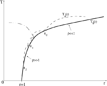
Figure 3: Examples of graviton trajectories in the bulk (dashed line). The brane trajectory, with relativistic matter, is also shown (continuous line).

All these gravitons contribute to an effective bulk energy-momentum tensor, which can be written as

$$T^{\rm(bulk)}_{AB}=\int d^{5}p\ \delta\left(p_{M}p^{M}\right)\sqrt{-g}\,f\,p_{A}p_{B},,$$ (31)

where $f$ is the phase space distribution function.

From the 5D Einstein equations, one can derive effective 4D Einstein equations [18], which in the homogeneous case yield

• the Friedmann equation

  $$H^{2}={8\pi G\over 3}\left[\left(1+{\rho\over 2\sigma}\right)\rho+\rho_{\rm{D}}\right],$$ (32)

• the non-conservation equation for brane matter, which must be identified with (29),

  $$\dot{\rho}+3\,H\,\left(\rho+p\right)=2\,{T^{\rm(bulk)}}_{RS}\,n^{R}\,u^{S}\,,$$ (33)

  where $n^{A}$ is the unit vector normal to the brane and $u^{A}$ its velocity in the bulk;

• the non-conservation equation for the “dark” component $\rho_{\rm{D}}$ (which includes all effective contributions from the bulk):

  $$\dot{\rho}_{\rm{D}}+4H\rho_{\rm{D}}=-2\left(1+{\rho\over\sigma}\right)T^{\rm(bulk)}_{AB}u^{A}n^{B}-2H\ell\,T^{\rm(bulk)}_{AB}n^{A}n^{B}\,.$$ (34)

On the right hand side of this last equation, we find two terms involving the bulk energy-momentum tensor: the first term, due to the energy flux from the brane into the bulk, contributes positively and thus increases the amount of dark radiation whereas the second term, due to the pressure along the fifth dimension, decreases the amount of dark radiation. These terms can be estimated numerically [19]. A striking property is that the gravitons coming back onto the brane and bouncing off it give a significant contribution to the transverse pressure effect, which almost, although not quite, compensates the flux effect. The evolution of the dark radiation, or rather its ratio with respect to the brane radiation density $\epsilon_{D}\equiv\rho_{D}/\rho$, is plotted on Fig. 4.

Figure 4: Evolution of the ratio $\epsilon_{D}=\rho_{D}/\rho$ for different values of the initial energy density on the brane $\rho_{i}$ (in units of $\sigma^{4}$).

One observes that at late times, i.e. far in the low energy regime, the ratio reaches a plateau, because the right hand side of (34) becomes negligible. The dark component then scales exactly like radiation.

4.2 Observational constraints

The computed amount of dark radiation can be confronted to observations. Indeed, since dark radiation behaves as radiation, it must satisfy the nucleosynthesis constraint on the number of additional relativistic degrees of freedom, usually expressed in terms of the extra number of light neutrinos $\Delta N_{\nu}$. The relation between $\Delta N_{\nu}$ and $\epsilon_{D}$ is given by

$$\epsilon_{D}={7\over 43}\left({g_{*}\over g_{*}^{\rm nucl}}\right)^{1/3}\Delta N_{\nu},$$ (35)

where $g_{*}^{\rm nucl}=10.75$ is the number of degrees of freedom at nucleosynthesis (in fact before the electron-positron annihilation). Assuming $g_{*}=106.75$ (standard model), this gives $\epsilon_{D}\simeq 0.35\Delta N_{\nu}$. The typical constraint from nucleosynthesis $\Delta N_{\nu}\lesssim 0.2$ thus implies

$$\epsilon_{D}\equiv{\rho_{D}\over\rho_{r}}\lesssim 0.03\left({g_{*}\over g_{*}^{\rm nucl}}\right)^{1/3},$$ (36)

which gives $\epsilon_{D}\lesssim 0.09$ with the degrees of freedom of the standard model.

5 Brane inflation

In brane cosmology, the famous horizon problem is much less severe than in standard cosmology, because the gravitational horizon, associated with the signal propagation in the bulk, can be much bigger than the standard photon horizon, associated with the signal propagation on the brane[20]. However, it is still alive because the energy density on the brane is limited by the Planck limit $\rho\sim M^{4}$. Thus, one must still invoke inflation, altough alternative ideas based on the collision of branes[21] have been actively explored (however, the generation of a quasi-scale-invariant fluctuation spectrum, as required by observations, remains problematic).

The simplest way to get inflation in the brane is to detune the brane tension from its Randall-Sundrum value (6) in order to obtain a net effective four-dimensional cosmological constant that is positive. This leads to exponential expansion on the brane. In the GN coordinate system, the metric is separable and can be written as

$$ds^{2}=A(y)^{2}\left(-dt^{2}+e^{2Ht}d{\vec{x}}^{2}\right)+dy^{2},$$ (37)

with

$$A(y)=\cosh\mu y-\left(1+{\rho\over\sigma}\right)\sinh\mu|y|.$$ (38)

As in the Randall-Sundrum case, the linearized Einstein equations for the tensor modes lead to a separable wave equation. The shape along the fifth dimension of the corresponding massive modes is governed by the Schrödinger-like equation

$${d^{2}\Psi_{m}\over dz^{2}}-V(z)\Psi_{m}=-m^{2}\Psi_{m}\,,$$ (39)

after introducing the new variable $z-z_{b}=\int_{0}^{y}d\tilde{y}/A(\tilde{y})$ (with $z_{b}=H^{-1}\sinh^{-1}(H\ell)$) and the new function $\Psi_{m}=A^{-1/2}u_{m}(y)$. The potential is given by

$$V(z)={15H^{2}\over 4\sinh^{2}(Hz)}+{{9\over 4}}H^{2}-{3\over\ell}\left(1+{\rho\over\sigma}\right)\delta(z-z_{\rm b})\,$$ (40)

and plotted in Fig. 5.

Figure 5: Potential for the graviton modes in a de Sitter brane

In constrast with the Randall-Sundrum potential, the potential goes asympotically to the non-zero value $9H^{2}/4$. This indicates the presence of a gap between the zero mode ($m=0$) and the continuum of Kaluza-Klein modes ($m>3H/2$).

In practice, inflation is not strictly de Sitter but the de Sitter case discussed above is a good approximation when $\dot{H}\ll H^{2}$. To get “realistic” inflation in the brane, two main approaches have been considered: either to assume a five-dimensional scalar field which induces inflation in the brane[22], or to suppose a four-dimensional scalar confined on the brane[23].

In the latter case, the cosmological evolution during inflation is obtained by substituting the energy density $\rho_{\phi}=\dot{\phi}^{2}/2+V(\phi)$ in the modified Friedmann equation (26). For slow-roll inflation, this can be approximated by

$$H^{2}\simeq{8\pi G\over 3}\left(1+{V\over 2\sigma}\right)V.$$ (41)

Interestingly, because of the modified Friedmann equation, new features appear at high energy ($V>\sigma$): the slow-roll conditions are changed and, because the Hubble parameter is bigger than the standard value, yielding a higher friction on the scalar field, inflation can occur with potentials usually too steep to sustain it [24].

The scalar and tensor spectra generated during inflation driven by a brane scalar field have also been computed [23, 25]. They are modified with respect to the standard results:

$$P_{S}=P_{S}^{\rm(4D)}\left(1+{V\over 2\sigma}\right)^{3},\qquad P_{T}=P_{T}^{\rm(4D)}F^{2}(H\ell),$$ (42)

with

$$F\!\left(x\right)=\left\{\sqrt{1+x^{2}}-x^{2}\ln\left[{1\over x}+\sqrt{1+{1\over x^{2}}}\right]\right\}^{\!\!-1/2}\!.$$ (43)

$F\simeq 1$ at low energies, i.e. for $H\ell\ll 1$, whereas $F\simeq{(3/2)H\ell}\sim V/\sigma$ at very high energies, i.e. for $H\ell\gg 1$. At low energies, $F\simeq 1$ and one recovers exactly the usual four-dimensional result but at higher energies the multiplicative factor $F$ provides an enhancement of the gravitational wave spectrum amplitude with respect to the four-dimensional result. However, comparing this with the amplitude for the scalar spectrum, one finds that, at high energies ($\rho\gg\sigma$), the tensor over scalar ratio is in fact suppressed with respect to the four-dimensional ratio. However, a difficult question is how the perturbations will evolve during the subsequent cosmological phases, the radiation and matter eras.

6 Beyond homogeneous brane cosmology

The homogeneous and isotropic brane cosmology is in fact very simple because of the generalized Birkhoff’s theorem mentioned earlier. But, when the cosmological symmetry is relaxed, things become rather difficult because the bulk geometry is no longer Schwarzschild-AdS. This section presents some aspects of this complexity, starting with anisotropic, but still homogeneous, models and then discussing the evolution of the linear cosmological perturbations.

6.1 Anisotropic brane cosmology

Let us now discuss configurations where the cosmology in the brane is homogeneous but anisotropic, e.g. of the Bianchi I type with a metric of the form

$$ds^{2}_{b}=-d\tau^{2}+\sum_{i=1}^{3}a_{i}^{2}(\tau)(dx^{i})^{2}.$$ (44)

Although many works in the literature have been devoted to this subject, most of them use the effective four-dimensional equations projected on the brane. It is a more challenging task to solve the 5D Einstein equations for the bulk as well, starting e.g. from an ansatz of the form

$$ds_{\rm bulk}^{2}=-{n^{2}(t,y)}dt^{2}+\sum_{i=1}^{3}{a_{i}^{2}(t,y)}({dx^{i}})^{2}+dy^{2}.$$ (45)

Assuming that the metric is separable, it turns out that analytical solutions can be obtained [26]. The five-dimensional metric is given by

$$ds^{2}=\sinh^{1/2}(4y/\ell)\left[\right. - \tanh\left(2y/\ell\right)^{2q_{0}}dt^{2}$$ (46)

$$+ \left.\sum_{i}\tanh\left(2y/\ell\right)^{2q_{i}}t^{2p_{i}}\left(dx^{i}\right)^{2}\right]+dy^{2},$$ (47)

where the seven coefficients $q_{\mu}$ and $p_{i}$ must satisfy the constraints

$$\sum_{\mu=0}^{3}q_{\mu}=0,\quad\sum_{\mu}q_{\mu}^{2}={3\over 4},\quad\sum_{i=1}^{3}p_{i}=1,\quad\sum_{i}p_{i}^{2}=1,\quad\sum_{i}q_{i}\left(p_{i}+1\right)=0.$$ (48)

In general, a brane embedded in an anisotropic bulk spacetime must contain matter with anisotropic stress, because of the junction conditions:

• isotropic part:

  $$n^{-1}\dot{y}_{b}\left.\dot{A}\right|_{b}+\sqrt{1+\dot{y}_{b}^{2}}\,\left.{A^{\prime}}\right|_{b}=\frac{\kappa^{2}}{6}\rho_{b},$$ (49)

• anisotropic part:

  $$n^{-1}\dot{y}_{b}\left.\dot{B}_{i}\right|_{b}+\sqrt{1+\dot{y}_{b}^{2}}\;\left.{B^{\prime}}_{i}\right|_{b}=\frac{\kappa^{2}}{2}\pi_{i},$$ (50)

  where $\pi_{i}$ is the anisotropic pressure in the brane,

with the notation $3A\equiv\ln(a_{1}a_{2}a_{3})$ and $B_{i}\equiv\ln a_{i}-A$. Note that the brane position $y_{b}$ is not assumed to be fixed here: in this sense the coordinate system is not Gaussian Normal. Interestingly, the above solutions include a particular bulk geometry, for $q_{0}=\pm\sqrt{3}/4$, in which one can embed a moving brane with perfect fluid as matter. The effective cosmological equation of state $P_{\rm eff}/\rho_{\rm eff}$ is negative but goes to zero at late times.

6.2 Scalar cosmological perturbations

A crucial step for brane cosmology is to be confronted with cosmological observations, in particular the CMB fluctuations. Although the primordial power spectra for scalar and tensor perturbations have been computed, the subsequent evolution of the cosmological perturbations is non trivial and has not been fully solved yet. The reason for this is that, in contrast with standard cosmology where the evolution of cosmological perturbations can be reduced to ordinary differential equations for the Fourier modes, the evolution equations in brane cosmology are partial differential equations with two variables: time and the fifth coordinate. Another delicate point is to specify the boundary conditions, both in time and space.

An instructive, although limited, approach for the brane cosmological perturbations is the brane point of view, based on the 4D effective Einstein equations on the brane, usually written in the form [18]

$$G_{\mu\nu}+\Lambda_{4}g_{\mu\nu}=8\pi G\tau_{\mu\nu}+\kappa^{2}\Pi_{\mu\nu}-E_{\mu\nu},$$ (51)

where $\tau_{\mu\nu}$ is the brane energy-momentum tensor, $\Pi_{\mu\nu}$ is a tensor depending quadratically on $\tau_{\mu\nu}$, giving in particular the $\rho^{2}$ term in the Friedmann equation, and $E_{\mu\nu}$, which corresponds to the dark radiation in the homogeneous case, is the projection on the brane of the bulk Weyl tensor.

It is then a straightforward exercise, starting from (51), to write down explicitly the perturbed effective Einstein equations on the brane, which will look exactly as the four-dimensional ones for the geometrical part but with extra terms due to $\Pi_{\mu\nu}$ and $T^{Weyl}_{\mu\nu}$ . One thus gets equations relating the perturbations of the metric to the matter perturbations and the perturbations of the projected Weyl tensor, which formally can be assimilated to a virtual fluid, with corresponding (perturbed) energy density $\rho_{E}+\delta\rho_{E}$, pressure $P_{E}+\delta P_{E}={1\over 3}(\rho_{E}+\delta\rho_{E})$ and anisotropic pressure. The contracted Bianchi identities ($\nabla_{\mu}G^{\mu}_{\nu}=0$) and energy-momentum conservation for matter on the brane ($\nabla_{\mu}\tau^{\mu}_{\nu}=0$) ensure, using Eq. (51), that

$$\nabla_{\mu}E^{\mu}_{\nu}=\kappa^{4}\,\nabla_{\mu}\Pi^{\mu}_{\nu}\,.$$ (52)

In the background, this tells us that $\rho_{E}$ behaves like radiation, as we knew already, and for the first-order perturbations, one finds that the effective energy of the projected Weyl tensor is conserved independently of the quadratic energy-momentum tensor. The only interaction is a momentum transfer.

It is also possible to construct [27] gauge-invariant variables corresponding to the curvature perturbation on hypersurfaces of uniform density, both for the brane matter energy density and for the total effective energy density (including the quadratic terms and the Weyl component). These quantities are extremely useful because their evolution on scales larger than the Hubble radius can be solved easily. However, their connection to the large-angle CMB anisotropies involves the knowledge of anisotropic stresses due to the bulk metric perturbations. This means that for a quantitative prediction of the CMB anisotropies, even at large scales, one needs to determine the evolution of the bulk perturbations.

In summary, one can obtain a set of equations for the brane linear perturbations, where one recognizes the ordinary cosmological equations but modified by two types of corrections:

• modification of the homogeneous background coefficients due to the additional $\rho^{2}$ terms in the Friedmann equation. These corrections are negligible in the low energy regime $\rho\ll\sigma$;

• presence of source terms in the equations. These terms come from the bulk perturbations and cannot be determined solely from the evolution inside the brane. To determine them, one must solve the full problem in the bulk (which also means to specify some initial conditions in the bulk).

One should also mention a very recent work [28] on the post-inflation evolution of gravitational waves, which indicates that, on very small scales, the spectral density of gravitational waves is reduced with respect to the standard 4D result.

7 Conclusions

In this contribution, I have presented some aspects of brane-world models, covering both the (static) Randall-Sundrum model and its cosmological extensions. Due to lack of time/space, I have not discussed many other interesting topics in the field. Examples are the brane cosmology of models involving Gauss-Bonnet corrections; the induced gravity models, where one includes a 4D Einstein-Hilber action for the brane and which can lead to late-time cosmological effects mimicking dark energy.

There are still many open questions in brane cosmology. Even in the simplest set-up, discussed here, based on a cosmological extension of the Randall-Sundrum model, the evolution of cosmological perturbations has not yet been solved, although some significant progress has been made. The situation is still more complicated in more sophisticated models, involving a bulk scalar field and/or collision of branes. It must be emphasized that the predictions for the cosmological perturbations, as observed in the CMB experiments, and their adequation with the present data, is a crucial test for brane-world models for which the early universe is modified. More direct tests of brane-world models involve gravity experiments or collider experiments. However, if the fundamental Planck mass is too high, such direct experiments cannot see extra-dimensional effects and one must turn to cosmology to try to see indirect signatures from the early universe.

Another direction of research is to make contact between the brane-worlds, which are still only phenomenological models, and a fundamental theory like string theory.

References

- [1] C. D. Hoyle, D. J. Kapner, B. R. Heckel, E. G. Adelberger, J. H. Gundlach, U. Schmidt and H. E. Swanson, Phys. Rev. D 70, 042004 (2004) [arXiv:hep-ph/0405262].
- [2] N. Arkani-Hamed, S. Dimopoulos and G. R. Dvali, Phys. Lett. B 429, 263 (1998) [arXiv:hep-ph/9803315].
- [3] L. Randall and R. Sundrum, Phys. Rev. Lett. 83 (1999) 3370 [arXiv:hep-ph/9905221].
- [4] L. Randall and R. Sundrum, Phys. Rev. Lett. 83 (1999) 4690 [arXiv:hep-th/9906064].
- [5] V. A. Rubakov, Phys. Usp. 44, 871 (2001) [Usp. Fiz. Nauk 171, 913 (2001)] [arXiv:hep-ph/0104152]; D. Langlois, Prog. Theor. Phys. Suppl. 148, 181 (2003) [arXiv:hep-th/0209261]; F. Quevedo, Class. Quant. Grav. 19, 5721 (2002) [arXiv:hep-th/0210292]. P. Brax and C. van de Bruck, Class. Quant. Grav. 20, R201 (2003) [arXiv:hep-th/0303095]; R. Maartens, Living Rev. Rel. 7, 1 (2004) [arXiv:gr-qc/0312059]; P. Brax, C. van de Bruck and A. C. Davis, arXiv:hep-th/0404011.
- [6] J. Garriga and T. Tanaka, Phys. Rev. Lett. 84 (2000) 2778 [arXiv:hep-th/9911055].
- [7] T. Tanaka, Prog. Theor. Phys. Suppl. 148, 307 (2003) [arXiv:gr-qc/0203082].
- [8] R. Emparan, A. Fabbri and N. Kaloper, JHEP 0208, 043 (2002) [arXiv:hep-th/0206155].
- [9] S. Kanno and J. Soda, Phys. Rev. D 66, 083506 (2002) [arXiv:hep-th/0207029].
- [10] W. D. Goldberger and M. B. Wise, Phys. Rev. Lett. 83 (1999) 4922 [arXiv:hep-ph/9907447].
- [11] P. Binétruy, C. Deffayet, U. Ellwanger and D. Langlois, Phys. Lett. B 477 (2000) 285 [arXiv:hep-th/9910219].
- [12] P. Binétruy, C. Deffayet and D. Langlois, Nucl. Phys. B 565 (2000) 269 [arXiv:hep-th/9905012].
- [13] C. Csaki, M. Graesser, C. F. Kolda and J. Terning, Phys. Lett. B 462, 34 (1999) [arXiv:hep-ph/9906513]; J. M. Cline, C. Grojean and G. Servant, Phys. Rev. Lett. 83, 4245 (1999) [arXiv:hep-ph/9906523].
- [14] P. Kraus, JHEP 9912 (1999) 011 [arXiv:hep-th/9910149].
- [15] D. Ida, JHEP 0009, 014 (2000) [arXiv:gr-qc/9912002]
- [16] D. Langlois, L. Sorbo and M. Rodriguez-Martinez, Phys. Rev. Lett. 89, 171301 (2002) [arXiv:hep-th/0206146].
- [17] A. Hebecker and J. March-Russell, Nucl. Phys. B 608, 375 (2001) [arXiv:hep-ph/0103214].
- [18] T. Shiromizu, K. i. Maeda and M. Sasaki, Phys. Rev. D 62, 024012 (2000) [arXiv:gr-qc/9910076].
- [19] D. Langlois and L. Sorbo, Phys. Rev. D 68, 084006 (2003) [arXiv:hep-th/0306281].
- [20] R. R. Caldwell and D. Langlois, Phys. Lett. B 511, 129 (2001) [arXiv:gr-qc/0103070].
- [21] J. Khoury, B. A. Ovrut, P. J. Steinhardt and N. Turok, Phys. Rev. D 64 (2001) 123522 [arXiv:hep-th/0103239].
- [22] Y. Himemoto and M. Sasaki, Phys. Rev. D 63, 044015 (2001) [arXiv:gr-qc/0010035].
- [23] R. Maartens, D. Wands, B. A. Bassett and I. Heard, Phys. Rev. D 62, 041301 (2000) [arXiv:hep-ph/9912464].
- [24] E. J. Copeland, A. R. Liddle and J. E. Lidsey, Phys. Rev. D 64, 023509 (2001) [arXiv:astro-ph/0006421].
- [25] D. Langlois, R. Maartens and D. Wands, Phys. Lett. B 489, 259 (2000) [arXiv:hep-th/0006007].
- [26] A. Fabbri, D. Langlois, D. A. Steer and R. Zegers, JHEP 0409, 025 (2004) [arXiv:hep-th/0407262].
- [27] D. Langlois, R. Maartens, M. Sasaki and D. Wands, Phys. Rev. D 63, 084009 (2001) [arXiv:hep-th/0012044].
- [28] K. Ichiki and K. Nakamura, arXiv:astro-ph/0406606.