Phenomenology of Brane-World Cosmological Models
Abstract
We present a brief review of brane-world models —
models in which our observable Universe with its standard matter
fields is assumed as localized on a domain wall (three-brane) in a
higher dimensional surrounding (bulk) spacetime. Models of this
type arise naturally in M-theory and have been intensively studied
during the last years. We pay particular attention to the
covariant projection approach, the Cardassian scenario, to induced
gravity models, self-tuning models and the Ekpyrotic scenario. A
brief discussion is given of their basic properties and their
connection with conventional FRW cosmology.
PACS numbers: 04.50.+h, 11.25.Mj, 98.80.Jk
1 Introduction
In the brane-world picture, it is assumed that ordinary matter (consisting of the fields and particles of the Standard Model) is trapped to a three-dimensional submanifold (a three-brane) in a higher dimensional (bulk) spacetime. This world-brane is identified with the currently observable Universe. Such kind of scenarios are inspired by string theory/M-theory. One of the first examples of this type was the Hoava-Witten setup [1] of dimensional M-theory compactified on an orbifold (i.e. a circle folded on itself across a diameter). In this setup, gauge fields are confined to two dimensional planes/branes located at the two fixed points of the orbifold. In the low-energy limit, the symmetry is down-broken to the group of the Standard Model. Simultaneously, the brane is endowed with the structure of a product manifold consisting of a noncompact real 3D manifold and a compact real 6D manifold with the complex structure of a Calabi-Yau threefold and a characteristic compactification scale . When the distance between the planes is much larger than the compactification scale, , then the degrees of freedom can be integrated out (see e.g. [2]) and one arrives at an effective 5-D heterotic M-theory with two dimensional planes.

One of these planes describes our brane/Universe and the other one corresponds to a hidden brane (see Fig. 1). In the formal limit , one obtains a model with a single brane.
The described scenario is one of the possible scenarios for an embedding of branes into a higher-dimensional bulk manifold. Because up to now only certain aspects of the underlying fundamental higher dimensional theory are understood, the model building process is still going on and an uncovering of new aspects of brane nucleation/embedding mechanisms can be expected also for the future.
The presently known brane world models can be distinguished by the number of branes involved, their co-dimensions, as well as the topological structure of the branes and the higher dimensional bulk spacetime. One of the basic tests that any brane-world model has to pass, is the test on its compatibility with observable cosmological data and their implications. From the large number of currently present scenarios we select in the present mini-review only a few ones — to illustrate some of the possible deviations from usual FRW cosmology. The aim of the brief discussion is twofold. Firstly, for each of the selected models we briefly review the modifications of the Friedmann-like cosmological equations and demonstrate the regimes where the corresponding physics coincides with conventional FRW cosmology; and, secondly, we briefly indicate the type of observable deviations from it.
2 4D projected equations along the brane
Let us consider a single brane embedded in a five-dimensional bulk spacetime. Denoting the Gaussian normal (fifth) coordinate orthogonal to the brane by we assume the brane position at some fixed position which without loss of generality can be set as . Furthermore, we assume that there is bulk matter present in 5D and 4D matter on the brane. denotes the bulk cosmological constant and the cosmological constant on the brane (the brane tension). The 5D Einstein equations for this system read
| (1) |
The components along the brane can be easily derived by projecting out the normal components. With the ansatz , where is the unit normal to the surface (brane) at , the metric can be split as
| (2) |
The Gauss-Codazzi equations yield then the effective 4D Einstein equations along the brane (for the details we refer to [3] and the reviews [4, 5])
| (3) | |||||
where
| (4) |
is the contribution of the bulk matter,
| (5) |
— the projection of the bulk Weyl tensor (orthogonal to ) and
| (6) |
— the extrinsic curvature of the surface .
The on-brane matter can be taken into account via the Israel junction condition
| (7) |
Substitution of this condition into Eq. (3) yields the induced field equation on the brane:
| (8) |
The underlined terms are the specific brane-world contributions which are not present in usual general relativity. The first of these terms,
| (9) |
describes local bulk effects (local, because it depends only on the matter on the brane). The corresponding quadratic corrections follow from the quadratic extrinsic curvature terms in Eq. (3) and the Israel junction condition (7). The second and third underlined terms represent non-local bulk effects, with the traceless contribution playing the role of a dark radiation on the brane. The 4D effective cosmological and gravitational constants are defined as
| (10) |
From the latter relation we are lead (for this concrete type of models) to the following three conclusions. Firstly, only on positive-tension branes gravity has the standard sign . A negative tension brane with would correspond to an anti-gravity world. Secondly, the on-brane matter gives a linear contribution to the generalized gravity equations (8) only in the case of a non-vanishing brane tension. A vanishing brane tension implies via vanishing effective gravitational constant a vanishing linear energy-momentum contribution, , so that only quadratic terms will remain — what would spoil a transition to conventional cosmology in this limit. Thirdly, Eq. (8) reproduces standard Einstein gravity in the simultaneous limit , for kept fixed and .
Furthermore, it can be shown that for absent bulk matter () there will be no leakage of usual matter from the brane into the bulk,
| (11) |
and that in this case the on-brane Bianchi identities set the following constraint on the dark radiation:
| (12) |
Cosmological implications of the model are most easily studied with the help of a perfect fluid ansatz for the on-brane energy momentum tensor (EMT)
| (13) |
Assuming, furthermore, a natural equation of state for the dark radiation, , the corresponding energy momentum contribution can be approximated as
| (14) |
Substitution of Eqs. (13) and (14) into Eq. (8) shows that it is convenient to introduce an effective perfect fluid with total energy density and pressure
| (15) |
and an effective equation of state
| (16) |
where . The second and the third terms in Eqs. (15) correspond to local and non-local bulk corrections. These corrections will be small (and Eq. (16) will tend to the ordinary equation of state ) in the limit of a large brane tension and a small energy density of the dark radiation: . One expects this to happen, e.g., during late-time stages of the evolution of the Universe. The considered brane-world model predicts strong deviations from conventional cosmology in the high-energy limit. Assuming that the phenomenological description via Eqs. (8), (15), (16) is still applicable to energy densities at early evolution stages of the Universe, one obtains equation of state parameters (i.e. for and for ) which would imply inflation regimes quite different from those in usual 4D FRW models. We will demonstrate this fact explicitly below.
First, endowing the brane with a FRW metric, we express the conservation equations (11) and (12) in terms of the energy densities:
| (17) |
and
| (18) |
where, as usual, the Hubble constant is given as , and overdots denote derivatives with respect to the synchronous/cosmic time on the brane.
Subsequently, we restrict our attention to the simplest case of a model without bulk matter and dark radiation (a model with vanishing projection of the bulk Weyl tensor onto the brane). Then the generalized Friedmann equation is of the type
| (19) |
As above, we underlined the specific local bulk-induced contribution which is responsible for the deviation from the standard Friedmann equation222Here, the standard Friedmann equation follows from general relativity with -term.. Again, we observe that this deviation becomes dominant in the high-energy limit , whereas conventional cosmology is reproduced at late times when .
In the simple case of a flat brane with vanishing effective cosmological constant (compensation of brane tension and on-brane effects of the bulk cosmological constant according to Eq. (10)) the solution of Eq. (19) is easily found explicitly (see [6]) as:
| (20) |
At early times the scale factor behaves as , whereas for late times the conventional FRW behavior is restored: . Here, the parameters of the model should be chosen in such a way that the transition to conventional cosmology occurs before BBN.
As next, we briefly analyze the influence of the additional contributions of local bulk effects in Eqs. (8) and (19) on inflation. We demonstrate the basic effect with the help of the same simple flat-brane model as above — assuming that the energy density and pressure in the state equation are those of a homogeneous minimally coupled scalar field which lives on the brane: , . The conservation equation (11) is then equivalent to the field equation . For the Friedmann equation one gets
| (21) | |||||
in the high energy limit and
| (22) | |||||
in the limit of a conventional FRW setup (i.e. in the formal limit ). In these equations, the gravitational constant has been expressed in terms of the Planck mass, , with denoting the Newton constant. The important point is the relation between the slow-roll parameters and corresponding to these two limiting cases
| (23) |
During inflation the high-energy limit with holds so that and the local bulk corrections lead to a strong relaxation of the slow-roll conditions [7]. Additionally we note that the deviation of the cosmological equation (21) from the conventional one (22) will necessarily lead to a measurable imprint in the CMB anisotropies (corresponding details are discussed, e.g., in Ref. [5]).
3 Induced gravity brane-world models
In the previous section, the 4D on-brane gravitational equations were obtained via the projection of the 5D curvature along the brane. Another approach is based on the assumption that 4D effective gravity for matter fields confined to the brane can be induced on the brane by interactions with 5D gravity in the bulk [8–15]. This results in an effective 4D scalar curvature term (as well as higher order curvature corrections) in the effective on-brane action functional. For models with vanishing bulk cosmological constant and brane tension it was shown by Dvali, Gabadadze and Porrati (DGP) [13] how quantum interactions can induce effective 4D on-brane gravity. In their setup, the values of the 5D and 4D gravitational constants do not dependent on each other, rather they define a characteristic length scale at which the gravitational attraction experienced by on-brane matter changes from 4D Newton’s law to that in 5D (see below). Cosmological implications of induced gravity models were considered in [10,12,14,16–19]. Subsequently, we describe specific issues of induced gravity cosmology along the lines of Refs. [18, 19].
Let us consider a model with the following action:
| (24) | |||||
where denotes the 4D brane333In this section, the brane is assumed as a boundary of a manifold. The theory can be easily extended to the case where is embedded into ., and is the vector field of the inner normal to the brane. The gravitational constants are given in energy units as: and . Variation of the action (24) with respect to the 5D bulk metric and the 4D induced metric yields:
| (25) |
and
| (26) |
where denotes the induced metric (2) on the brane and
| (27) |
Eq. (26) describes gravity on the brane and the underlined term defines the bulk correction which is new compared to general relativity. Let us roughly estimate the length scale at which this term becomes important. Clearly, it can be dropped when . Introducing the characteristic scales for , i.e. , and assuming as usual for cosmological applications , we find for this ratio . This means that the correction plays an essential role at length scales . Explicitly, one has the following estimates:
| (28) |
For energies GeV the characteristic length scale is of the order of the present horizon scale , for higher energies it is smaller, and for the dark energy scale eV it is much larger than . Hence, in the latter case and, in general, for GeV the corrections will be unobservable at present time. The crucial role of the distance can be demonstrated on the behavior of the Newtonian potential. In Refs. [13, 17], it was approximated as
| (29) |
(effective 4D Newtonian scaling) and as
| (30) |
i.e. at large distances the gravitational potential scales as in accordance with the laws of a 5D theory.
Let us now illustrate the cosmological implication of this scenario. For this purpose we consider the simplest model — a setup without bulk matter: . The Codazzi relation guarantees then the conservation of matter on the brane:
| (31) |
Here, is the covariant derivative associated with the induced metric (in normal Gaussian coordinates (2)) and we use the notations , . The complete trace of the Gauss relation yields
| (32) |
and plugging from Eq. (26) into this relation gives the following on-brane equations system:
| (33) |
Although these equations seem to form a closed system (they contain only on-brane quantities), the higher order derivatives allow for additional degrees of freedom which should be fixed via integration. One such term which reappears in the corresponding cosmological equations is the dark radiation. With the help of a perfect fluid ansatz (similar to that in the previous section), it was shown in Ref. [18] that integration of Eq. (3) yields:
| (34) |
where and is a constant of integration444It was shown in Ref. [18], that the generalized on-brane Friedmann equation (19) (obtained by the projection method of the previous section 2) can be recovered from Eq. (34) by the formal limit . For a model with symmetry and a brane embedded in the bulk (and not located on the bulk boundary as considered in the present section) this formal limit gives what via relations (10) exactly reproduces (19) with additional dark radiation term.. Obviously, the term can be identified as dark radiation. Assuming as before that the 5D and 4D gravitational constants and can be fixed independently, the solution of Eq. (34) can be resolved for the Hubble parameter,
| (35) |
where .
Again, the dynamics of on-brane matter depends on the characteristic length scale . At short distances , what corresponds to high energy densities, the bulk corrections play no important role. Eq. (35) shows that in the (UV) limit we restore the equation of conventional cosmology
| (36) |
In the particular case this happens already at555This characteristic energy density changes within the limits depending on the concrete value of from the interval . In the special case GeV it holds . .
In the opposite case of the IR limit with low energy densities (i.e. ) the bulk corrections become dominant. Depending on the sign in Eq. (35) two regimes can be distinguished. (Again, we perform the corresponding sketchy estimates for the simplest model with where the low energy density regime corresponds to .) In the first regime with ”minus” sign in Eq. (35) one finds
| (37) |
which formally coincides with the high energy limit in Eq. (19) of the previous section. The different numerical prefactors 1/9 in Eq. (37) and 1/36 in Eq. (19) are the result of different setups: in the previous section the brane was embedded into the bulk, whereas here it is a boundary of the bulk. For a flat brane, , the scale factor behaves non-conventionally: . One has to conclude that a Universe (brane-world) which is filled with ordinary matter (with ) undergoes no late time acceleration in this regime. The situation is completely different for models described by Eq. (35) with ”plus” sign. Here, the low energy density regime is necessarily connected with a dynamics of the type
| (38) |
Thus, in this scenario a phase of matter or radiation dominated cosmology is followed by a late phase of accelerated expansion [16].
A more detail analysis of the cosmological behavior in models with induced gravity can be found, e.g., in Refs. [17, 19]666It was shown in [19] that conventional on-brane dark matter can lead to a cosmology with equation of state parameter but without phantom-like future singularity as well as with a transient acceleration with subsequent matter dominated regime. Additionally, it should be noted that in spite of the appealing features of the DGP model, it predicts [20, 21] intensive and strong interactions at the energy scale , which for corresponds to distances km [20]. Obviously, this would conflict with experimental data. However, it was noted in Ref. [22] that this problem can be cured with the help of a proper UV completion of the theory and it may not occur for certain configurations of the general type (24) (with ) [20].. An interesting generalization of DGP-type models to branes with co-dimensions was proposed in Ref. [23]. In the case of a co-dimension 2 model, the characteristic scale at which gravity becomes six-dimensional is , which is of order of the Hubble radius for the dark energy mass scale eV. However, it was pointed out [24] that such models are not free of ghosts and will lead to violations of the equivalence principle.
4 Cardassian expansion
The discovery of the present late-time acceleration of the Universe posed a great puzzle to modern theoretical cosmology. Up to now several scenarios have been proposed as possible resolution, such as a cosmological constant, a decaying vacuum energy and quintessence. However, non of them is fully satisfactory. On the other hand, as we have seen above, a possible explanation could consist in an IR modification of gravity and with it in a modification of the effective Friedmann equation (see e.g. the low energy limit of Eq. (35)). A natural phenomenological ansatz for an effective Friedmann equation could consist, e.g., in adding a nonlinear term in the energy density,
| (39) |
where is a constant prefactor. Assuming the matter as dust with this would lead for a dominating nonlinear energy density term to
| (40) |
Thus, for the Universe would undergo an accelerated expansion. Therefore, for large energy densities the main contribution would come from the first term in Eq. (39) and one would recover conventional cosmology. In contrast to this, for small energy densities the second term would dominate so that starting from a certain evolution stage the Universe would undergo a late time acceleration. Such a scenario was dubbed ”Cardassian expansion”777The name Cardassian refers to a humanoid race in ”Star Trek” whose goal was to take over the Universe, i.e. an accelerated expansion. [25]. The appealing feature of this ansatz is in the fact that the acceleration is explained without involving vacuum energy. The question is how to derive the specific (phenomenological) nonlinear contributions in the energy density from a more fundamental theory (such as string theory/M-theory).
One possible way could consist in taking advantage of bulk corrections in brane-world models. For the special case with this has been demonstrated in the previous two sections. In Ref. [26] it was shown that, in general, it is possible for such models to get a modified Friedmann equation with any . The main idea consists in defining the bulk moduli and in the metric
| (41) |
in such a way that the energy density of on-brane dust behaves (via the Israel junction conditions) in accordance with Eq. (40). On the other hand, these moduli specify the bulk EMT via the 5D Einstein equations (see also [27]). The main drawback of the approach consists in a very clumsy and inelegant form of this bulk EMT [25, 26]. It is very difficult to guess what kind of matter could produce such an EMT. Furthermore, the combination with arbitrary is not yet obtained by this method. But precisely this combination is required to induce a matter dominated cosmology which is followed by a late phase of accelerated expansion (for ).
5 Self-tuning Universe
One of the most natural candidates for the dark energy causing the present late time acceleration of the Universe is a positive vacuum energy (in other words, a cosmological constant). The energy density of vacuum fluctuations (with natural cut-off ) can be estimated as
| (42) |
and is 123 orders of magnitude greater than the observable dark energy density . Usually, this discrepancy is resolved by an extra ordinary parameter fine tuning and for this reason it is well known as the fine tuning problem. However, there seems to exist a possibility to avoid this problem. The idea again consists in a modification of the Friedmann equation. Let us suppose that the standard (flat space) Friedmann equation is modified in such a way [28] that it holds
| (43) |
where is a smooth function of the energy density and the pressure , and dots denote subdominant terms of other type. Then the state equation of the vacuum energy, , shows that its contribution will exactly cancel and that it will not affect the evolution of the Universe, i.e. its energy density can be arbitrary large. In general, such a modification can be in agreement with modern observational data. It is easily demonstrated on the simplest model with
| (44) |
During the matter dominated stage with this equation reads . The additional factor 3/4 is rather close to 1 and such a deviation from the standard Friedmann equation is very difficult to extract from observational data. During the radiation dominated stage with the standard equation is restored, what is very important for the BBN. Scenarios with a modified Friedmann equation of the type (43) were dubbed ”self-tuning Universe”. They were first proposed in Refs. [29, 30] for specific brane-world models. An excellent explanation of the basic mechanisms underlying this setup was given in Ref. [28]. In our subsequent brief outline, we mainly follow this work.
The starting point for the scenarios is a 5D brane-world model with action
| (45) |
where is a dilatonic bulk field and are matter fields living on the brane. The 5D metric in the Einstein frame is connected with the 5D metric in Brans-Dicke (BD) frame as
| (46) |
with the induced metrics and connected by a similar relation. The setup allows for two possible types of brane-matter coupling in the effective 4D action on the brane: either the matter is coupled to the induced 4D metric in the BD frame,
| (47) |
or it is coupled to the induced metric in the Einstein frame,
| (48) |
Using the ansatz (41) for the 5D metric (in the Einstein frame) and the special parameter tuning
| (49) |
one finds the following on-brane equations
| (50) |
which contain energy-density—pressure combinations of a form similar to the self-tuning combinations of the generalized Friedmann equation (43). In (50) equation (I) corresponds to the BD frame coupling and equation (II) to the Einstein frame coupling. The tilded and non-tilded energy densities and pressures and are defined from Eqs. (47) and (48) with respect to metrics and , respectively. 0-subscripts refer to on-brane quantities.
Comparing equations (I) and (II) in (50) with the self-tuning equations (43) and (44), one immediately realizes that the quadratic energy-density—pressure term in Eq. (I) would yield a self-tuning but it would spoil the possibility for a limit to conventional cosmological behavior. In contrast to this, Eq. (II) can provide the necessary linear dependence. Splitting, for example, the on-brane energy density and pressure into a static background component (which can be identified with a vacuum contribution888The self-tuning scenario was designed to cancel the huge vacuum contributions, but in its current form it is not yet capable to elegantly induce accelerated expansion — like inflation or late-time acceleration (see also footnote 10).) and a dynamical component of ordinary (non-vacuum) matter,
| (51) |
(with as brane tension) one gets from Eq. (II) for constant on-brane values of the dilaton999Here, the stabilization problem for the on-brane value of the dilaton is left aside. It would require a separate investigation. an equation capable for a self-tuning
| (52) |
In a late-time regime, the term quadratic in the dynamical energy density and pressure would be subdominant and it remains to check whether the resulting linear model will be capable to reproduce conventional cosmology. The analysis can be made explicit, e.g., by considering the simplest case of a flat-brane ansatz for the metric (41)
| (53) |
The concrete form of was found in Refs. [29, 30] as
| (54) |
where corresponds to a boundary (opposite to the world-brane) at which the metric experiences a singularity, . The effective 4D gravitational constant on the brane can be obtained via dimensional reduction as
| (55) |
Thus, up to quadratic terms, Eq. (52) reads
| (56) |
and yields after integration
| (57) |
For a Universe which is dominated by a combination of dust () and radiation () this leads to a Hubble parameter of the type
| (58) |
with as constant of integration.
Obviously, the considered toy model does not exactly reproduce the dynamics of conventional cosmology. During the matter dominated stage the additional prefactor induces a deviation from conventional cosmology which probably will leave an imprint in the CMB anisotropy. Also the dynamics of the radiation dominated stage is governed by a different equation — which can affect the BBN. This may require a special tuning mechanism101010Additionally, it should be noted that up to now no convincing mechanism has been found for an elegant matching of the self-tuning scenarios with inflation. The point is that for conventional cosmology a vacuum equation of state with yields const. In contrast to this, setting in Eq. (52) (i.e., a vacuum of the dynamical contributions) gives and behaves in the same way as during the RD stage of conventional cosmology. to produce the correct light-element abundances. Nevertheless, the simple toy model allowed us to illuminate the main ideas of the self-tuning mechanism. Further details of the scenario have been worked out, e.g., in Refs. [31–34].
6 Ekpyrotic Universe
A very interesting scenario which is based on a different general setup — compared with those in the previous sections — was proposed in Ref. [35]. It is based on the assumption that the evolution of our Universe (in accordance with known observational data) can be explained with the help of a relatively simple brany M-theory setup with orbifold symmetry. The starting point is the Hoava-Witten model (briefly mentioned in the introduction section 1) which after dimensional reduction leads to an effective 5D action of the type
| (59) |
The scalar field defines the volume scale (modulus) of the Calabi-Yau three-fold and is the field strength of a four-form gauge field. The key point of this model is a static (nearly) Bogomol’nyi-Prasad-Sommerfeld (BPS) solution [35] which describes a setup consisting of three 3-branes:
| (60) | |||||
| (61) | |||||
where denotes the conformal time, is defined as
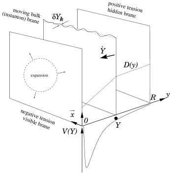
and are constants (with ). Two of the three branes are located at the orbifold fixed points and , whereas the third (bulk) brane is positioned at . Our visible brane (at ) is assumed to have negative tension , the hidden brane (at ) and the bulk brane to have a positive one. Furthermore, it is assumed that the bulk brane is nucleated near the positive tension (hidden) brane at . It is supposed that the bulk brane is very light: . A very important property of the (nearly) BPS solution is that all these three branes are flat and parallel one to the other.
Additionally, it is assumed that a non-perturbative interaction between the bulk and boundary branes leads to an effective potential
| (63) |
which for small suddenly becomes zero ( and are positive dimensionless parameters of the model). Via the potential the light bulk brane is attracted to the visible brane and moves adiabatically slowly towards the visible brane (see the schematic illustration in Fig. 2).
In this scenario, branes and bulk are assumed to start out from a cold, symmetric state with (6) which is nearly BPS. The beginning of our Universe, i.e. the Big Bang, is identified in this model with the impact of the bulk brane on the visible brane. After this collision, a part of the kinetic energy of the bulk brane transforms into radiation which is deposited in the three dimensional space of the visible brane. The scenario was called ”Ekpyrotic Universe” [35]111111This term was drawn from the Stoic model of cosmic evolution in which the Universe is consumed by fire at regular intervals and reconstituted out of this fire — a conflagration called ekpyrosis. In the present scenario, the Universe is made through a conflagration ignited by a brane collision.. An early detailed analysis of its features was performed in Refs. [35–41].
It was argued that this model could solve the main cosmological problems without invoking inflation and as alternative to it121212See, however, the critical comments in [36, 37] and the reply to these comments in [38].:
-
•
It is assumed that the monopole problem can be avoided if the parameters of the model are chosen in such a way that the temperature on the visible brane after collision is not high enough for a production of primordial monopoles.
-
•
The flatness and homogeneity problems are automatically solved131313For the solution of these problems in other brane world models, e.g. such with large extra dimensions, different smoothing mechanisms have been proposed [42]. because the nearly BPS branes are assumed as sufficiently flat and homogeneous (see however the critical comments in [36, 37] concerning the naturalness of the required high parameter tuning).
-
•
The horizon problem is solved by the extremely slow motion of the bulk brane so that, before collision, particles on the visible brane can travel an exponentially long distance. As result, the horizon distance can be much bigger than the Hubble radius at collision , where is the temperature of the visible brane at collision.
-
•
It is assumed that the large-scale structure on the visible brane is induced by quantum fluctuations (ripples) in the position of the bulk brane. These fluctuations would lead to a space-dependent time delay in the brane collision which on its turn would result in density fluctuations on the visible brane. Because small ripples can generate a large time delay, the collision could induce a spectrum of density fluctuation which would extend to exponentially large, super-horizon scales. In the considered scenario, the spectrum of perturbations is approximately scale invariant. However, in the simplest variant of the Ekpyrotic model the spectrum of adiabatic fluctuations is blue [39, 40].
Summarizing, the M-theory based scenario of an Ekpyrotic Universe has a large number of interesting features which could present an alternative to inflation. Future investigations will show which of the scenarios is more robust. Further developments in this direction can be found, e.g., in Refs. [43, 44].
7 Conclusion
We are living in very interesting time because new observational data directly indicate that our knowledge about the Universe and its evolution is in great extent limited. In this situation new ideas and new theoretical models are required to explain the observational data. In their turn, these new models will predict new observable phenomena which can be used as test tools to single out those scenarios which are most close to nature. One possible direction to modify the currently accepted standard theory of cosmology are brane-world models — M-theory inspired setups in which our observable Universe is interpreted as a 3D submanifold embedded in a higher dimensional bulk spacetime. The aim of the present mini-review was to give a very brief description of some of the basic features of these models — illustrating them with the help of a few concrete toy model setups.
Acknowledgments
We thank the High Energy,
Cosmology and Astroparticle Physics Section of the ICTP (Trieste)
for their warm hospitality during the preparation of this
mini-review as well as for financial support from the Associate
Scheme (A.Z.) and from HECAP (U.G.). Additionally, U.G.
acknowledges support from DFG grant KON/1806/2004/GU/522.
References
- [1] P. Hoava and E. Witten, Nucl. Phys., B460, 506 - 524 (1996), hep-th/9510209; ibid., B475, 94 - 114 (1996), hep-th/9603142.
- [2] A. Lukas, B. A. Ovrut, K.S. Stelle and D. Waldram, Phys. Rev., D59, 086001 (1999), hep-th/9803235; A. Lukas, B. A. Ovrut and D. Waldram, Nucl. Phys., B532, 43 - 82 (1998), hep-th/9710208.
- [3] T. Shiromizu, K. Maeda and M. Sasaki, Phys. Rev., D62, 024012 (2000), gr-qc/9910076.
- [4] R. Maartens, Phys. Rev., D62, 084023 (2000), hep-th/0004166.
- [5] R. Maartens, Living Rev. Rel., 7, 1 - 99 (2004), gr-qc/0312059.
- [6] A. Campos and C. F. Sopuerta, Phys. Rev., D63, 104012 (2001), hep-th/0101060.
- [7] G. Huey and J. E. Lidsey, Phys. Lett., B514, 217 - 225 (2001), astro-ph/0104006.
- [8] M. Pavi, Grav. Cosmol., 2, 1 - 6 (1996), gr-qc/9511020.
- [9] S. Nojiri, S. D. Odintsov and S. Zerbini, Phys. Rev., D62, 064006 (2000), hep-th/0001192.
- [10] S.W. Hawking, T. Hertog and H.S. Reall, Phys. Rev., D62, 043501 (2000), hep-th/0003052.
- [11] H. Collins and B. Holdom, Phys. Rev., D62, 105009 (2000), hep-ph/0003173.
- [12] S. Nojiri and S. D. Odintsov, Phys. Lett., B484, 119 - 123 (2000), hep-th/0004097.
- [13] G.R. Dvali, G. Gabadadze and M. Porrati, Phys. Lett., B485, 208 - 214 (2000), hep-th/0005016.
- [14] Yu.V. Shtanov, preprint hep-th/0005193 (2000).
- [15] G.R. Dvali and G. Gabadadze, Phys. Rev., D63, 065007 (2001), hep-th/0008054.
- [16] C. Deffayet, Phys. Lett., B502, 199 - 208 (2001), hep-th/0010186.
- [17] C. Deffayet, G.R. Dvali and G. Gabadadze, Phys. Rev., D65, 044023 (2002), astro-ph/0105068.
- [18] Y V. Shtanov, Phys. Lett., B541, 177 - 182 (2002), hep-ph/0108153.
- [19] V. Sahni and Yu. Shtanov, JCAP, 0311, 014 (2003), astro-ph/0202346.
- [20] M. A. Luty, M. Porrati and R. Rattazzi, JHEP, 0309, 029 (2003), hep-th/0303116.
- [21] V.A. Rubakov, preprint hep-th/0303125 (2003).
- [22] A. Nicolis and R. Rattazzi, JHEP, 0406, 059 (2004), hep-th/0404159.
- [23] G. Dvali, G. Gabadadze, X. Hou and E. Sefusatti, Phys. Rev., D67, 044019 (2003), hep-th/0111266.
- [24] S.L. Dubovsky and V.A. Rubakov, Phys. Rev., D67, 104014 (2003), hep-th/0212222.
- [25] K. Freese and M. Lewis, Phys. Lett., B540, 1 - 8 (2002), astro-ph/0201229.
- [26] D.J.H. Chung and K. Freese, Phys. Rev., D61, 023511 (2000), hep-ph/9906542.
- [27] P. Binetruy, C. Deffayet and D. Langlois, Nucl. Phys., B565, 269 - 287 (2000), hep-th/9905012.
- [28] S. M. Carroll and L. Mersini, Phys. Rev., D64, 124008 (2001), hep-th/0105007.
- [29] N. Arkani-Hamed, S. Dimopoulos, N. Kaloper and Raman Sundrum, Phys. Lett., B480, 193 - 199 (2000), hep-th/0001197.
- [30] S. Kachru, M. B. Schulz and E. Silverstein, Phys. Rev., D62, 045021 (2000), hep-th/0001206; D62, 085003 (2000), hep-th/0002121.
- [31] S. M. Carroll and M. M. Guica, preprint hep-th/0302067 (2003).
- [32] H.-P. Nilles, A. Papazoglou and G. Tasinato, Nucl. Phys., B677, 405 - 429 (2004), hep-th/0309042.
- [33] J. E. Kim and H. M. Lee, Phys. Lett., B590, 1 - 7 (2004), hep-th/0309046.
- [34] H. M. Lee, Phys. Lett., B587, 117 - 120 (2004), hep-th/0309050.
- [35] J. Khoury, B. A. Ovrut, P. J. Steinhardt and N. Turok, Phys. Rev., D64, 123522 (2001), hep-th/0103239.
- [36] R. Kallosh, L. Kofman and A. D. Linde, Phys. Rev., D64, 123523 (2001), hep-th/0104073.
- [37] R. Kallosh, L. Kofman, A. Linde, and A. Tseytlin, Phys. Rev., D64, 123524 (2001), hep-th/0106241.
- [38] J. Khoury, B. A. Ovrut, P. J. Steinhardt and N. Turok, preprint hep-th/0105212.
- [39] D. H. Lyth, Phys. Lett., B524, 1 - 4 (2002), hep-ph/0106153.
- [40] R. Brandenberger and F. Finelli, JHEP, 0111, 056 (2001), hep-th/0109004.
- [41] J. Khoury, B. A. Ovrut, P. J. Steinhardt and N. Turok, Phys. Rev., D66, 046005 (2002), hep-th/0109050.
- [42] G. D. Starkman, D. Stojkovic and M. Trodden, Phys. Rev. Lett., 87, 231303 (2001), hep-th/0106143.
- [43] J. Khoury, B. A. Ovrut, N. Seiberg, P. J. Steinhardt and N. Turok, Phys. Rev., D65, 086007 (2002), hep-th/0108187.
- [44] P. J. Steinhardt and N. Turok, Phys. Rev., D65, 126003 (2002), hep-th/0111098.