Braneworld black hole gravitational lens: Strong field limit analysis

Abstract

In this paper, a braneworld black hole is studied as a gravitational lens, using the strong field limit to obtain the positions and magnifications of the relativistic images. Standard lensing and retrolensing situations are analyzed in a unified setting, and the results are compared with those corresponding to the Schwarzschild black hole lens. The possibility of observing the strong field images is discussed.

PACS numbers: 11.25.-w, 04.70.-s, 98.62.Sb

Keywords: Braneworld cosmology, Black hole, Gravitational lensing

1 Introduction

Gravitational lensing by ordinary stars and galaxies can be analyzed in the weak field approximation, i.e., only keeping the first non null term in the expansion of the deflection angle [1]. If the lens is a black hole, this approximation is only valid for photons with large impact parameter, so a full strong field treatment is needed instead. In the general case where the lens is a compact object with a photon sphere, besides the primary and secondary weak field images, two infinite sets of faint relativistic images are formed by photons that make complete turns (in both directions of rotation) around the black hole before reaching the observer. In the last few years, several works studying different strong field lensing scenarios appeared in the literature. Virbhadra and Ellis [2] made a numerical analysis, using an asymptotically flat metric, of the case where the lens is a Schwarzschild black hole situated in the center of the Galaxy, and in another paper [3] they investigated numerically the lensing by naked singularities. Fritelli, Kling and Newman [4] found an exact lens equation without any reference to a background metric and compared their results with those of Virbhadra and Ellis. In the Schwarzschild geometry, several authors [5] used a logarithmic approximation of the deflection angle as a function of the impact parameter, for light rays passing very close to the photon sphere, to treat strong field situations. This asymptotic approximation is the starting point of an analytical method for strong field lensing, called the strong field limit [6], which gives the lensing observables in a straightforward way. Eiroa, Romero and Torres [7] extended this method to Reissner-Nordström geometry, and Bozza [8] showed that it can be applied to any static spherically symmetric lens. It was subsequently used by Bhadra [9] to study a charged black hole lens of string theory, and by Petters [10] to analyze the relativistic corrections to microlensing effects produced by the Galactic black hole. Bozza and Mancini [11] applied the strong field limit to study the time delay between different relativistic images, showing that different types of black holes are characterized by different time delays, and Bozza [12] extended the strong field limit to analyze the case of quasi-equatorial lensing by rotating black holes.
In standard lensing situations, the lens is placed between the source and the observer. When the lens has a photon sphere and the observer is placed between the source and the lens, or the source is situated between the lens and the observer, two infinite sequences of images with deflection angles closer to odd multiples of $\pi$ are obtained, a situation called retrolensing. Holtz and Wheeler [13] recently analyzed the two stronger images for a black hole situated in the galactic bulge with the sun as source, and suggested retrolensing as a new mechanism for searching black holes. De Paolis et al. [14] considered the retrolensing scenario of the bright star S2 orbiting around the massive black hole at the galactic center. Eiroa and Torres [15] studied the case of a spherically symmetric retrolens, using the strong field limit to obtain the positions and magnifications of all images. De Paolis et al. [16] extended, using the strong field limit, the work of Holtz and Wheeler to slowly spinning Kerr black hole, restricting their treatment to the black hole equatorial plane. Bozza and Mancini [17] analyzed, in the strong field limit, standard lensing, retrolensing and intermediate situations under a unified formalism, and studied in detail the case of the star S2, suggesting the possibility of observing the relativistic images in the year 2018. For other works that considered related topics on strong field lensing, see Ref. [18].

Braneworld cosmologies, where the ordinary matter is on a three dimensional space called the brane, embedded in a larger space called the bulk in which only gravity can propagate, became popular in the last few years [19]. These models, proposed to solve the hierarchy problem, i.e., the difficulty in explaining why the gravity scale is 16 orders of magnitude greater than the electro-weak scale, have motivation in recent developments of string theory, known as M-theory. The presence of extra dimensions would affect the characteristics of black holes [20]. The possibility of the existence of primordial black holes in the simplest of braneworld scenarios, the Randall-Sundrum [21] models (a positive tension brane in a bulk with a negative cosmological constant) with one extra dimension, have been studied by Clancy, Guedens and Liddle [22]. They showed that black holes formed in the high energy epoch of this theory have a longer lifetime, due to a different evaporation law. Majumdar [23] found that the primordial black holes could have a growth of their mass through accretion of surrounding radiation during the high energy phase, increasing their lifetime. These black holes could have survived up to present times and have an induced four dimensional metric on the brane distinct from Schwarzschild metric. They also may be created in high energy collisions in particle accelerators and in cosmic rays [20]. The possibility that these primordial black holes could act as gravitational lenses was analyzed by Majumdar and Mukherjee [24]. They only considered the case of photons with small deflection angles in the standard lensing configuration. In another braneworld model Frolov, Snajdr and Stojkovic [25] calculated, using a weak field approximation, the deflection of light propagating in the brane produced by a small size black hole in the bulk.

In this paper, the strong field limit is applied to study the relativistic images produced by the braneworld black hole analyzed by Majumdar and Mukherjee [24] only for the weak field situation. Standard lensing and retrolensing are considered for the case of high alignment between the source, the lens and the observer, which is the case where the images are more prominent. In Sec. 2, the deflection angle is calculated for the braneworld black hole. In Sec. 3, the positions and magnifications of the relativistic images are obtained, and in Sec. 4 the results are compared with those corresponding to a four dimensional Schwarzschild black hole. Finally, in Sec. 5, some conclusions are shown. Units such that $c=\hbar=1$ are used throughout this work.

2 Deflection angle

Consider a static spherically symmetric black hole that acts as a gravitational lens, with metric of the form

$$ds^{2}=-f(x)dt^{2}+g(x)dx^{2}+h(x)d\Omega^{2},$$ (1)

where $x=r/r_{H}$ is the radial coordinate in units of the event horizon radius. This black hole will have a photon sphere, that corresponds to circular unstable photon orbits around it, which radius $x_{ps}$ is given by the greater positive solution of the equation:

$$\frac{h^{\prime}(x)}{h(x)}=\frac{f^{\prime}(x)}{f(x)},$$ (2)

where the prime means derivative with respect to $x$. Assuming an asymptotically flat geometry at infinite, the deflection angle of a photon coming from infinite is given as a function of the closest approach distance $x_{0}$ by [26]

$$\alpha(x_{0})=I(x_{0})-\pi,$$ (3)

with

$$I(x_{0})=\int_{x_{0}}^{\infty}2\left[\frac{g(x)}{h(x)}\right]^{1/2}\left[\frac{h(x)f(x_{0})}{h(x_{0})f(x)}-1\right]^{-1/2}dx.$$ (4)

There are two cases where the integral can be approximated by simple expressions. For photons with $x_{0}\gg x_{ps}>1$, which have small deflection angles, the integral is usually replaced by a Taylor expansion in terms of $1/x_{0}$, keeping only the first non null term. This approximation is called the weak field limit, and it is used in lensing by stars and galaxies [1], and also for the primary and secondary images, in the standard lensing configuration, with high alignment, for black hole lenses [6, 7]. The integral diverges when $x_{0}=x_{ps}$, and for $0<x_{0}-x_{ps}\ll 1$, its large value can be asymptotically approximated by a logarithmic function [8]. This case, which corresponds to large deflection angles, is called the strong field limit [6]. The treatment of intermediate situations is more difficult, because one cannot rely on simple approximations.

Here it is studied as a gravitational lens, in the strong field limit, the braneworld black hole considered as a primordial black hole in Refs. [22, 23], and as a gravitational lens, in the weak field limit, in Ref. [24]. This black hole is nonrotating and it has no charge, and its geometry is that of a Schwarzschild solution in five dimensions. The Randall-Sundrum II [21] braneworld model is adopted, consisting of a single positive tension brane with three spatial dimensions, embedded in a one dimensional bulk with negative cosmological constant. For the event horizon radius $r_{H}$ much smaller than the AdS radius $l$, this black hole is a good approximation, in the neighborhood of the event horizon, of a black hole formed from collapsed matter confined to the brane. The induced four dimensional metric on the brane is [22]

$$ds^{2}=-\left(1-\frac{r_{H}^{2}}{r^{2}}\right)dt^{2}+\left(1-\frac{r_{H}^{2}}{r^{2}}\right)^{-1}dr^{2}+r^{2}d\Omega^{2},$$ (5)

with the black hole horizon radius $r_{H}$ given by

$$r_{H}=\sqrt{\frac{8}{3\pi}}\left(\frac{l}{l_{4}}\right)^{1/2}\left(\frac{M}{M_{4}}\right)^{1/2}l_{4},$$ (6)

where $M$ is the black hole mass, and $l_{4}$ and $M_{4}$ are, respectively, the four dimensional Planck length and mass. Using the radial coordinate $x$ defined above, the metric functions are $f(x)=g(x)^{-1}=1-x^{-2}$ and $h(x)=x^{2}$. Then

$$I(x_{0})=2x_{0}^{2}\int_{x_{0}}^{\infty}\left[x^{4}(x_{0}^{2}-1)-x_{0}^{4}(x^{2}-1)\right]^{-1/2}dx,$$ (7)

which, with the substitution $u=1/x$, takes the form

$$I(x_{0})=2x_{0}\int_{0}^{1}\left(u^{4}-x_{0}^{2}u^{2}+x_{0}^{2}-1\right)^{-1/2}dx,$$ (8)

and it can be expressed as

$$I(x_{0})=\frac{2x_{0}}{\sqrt{x_{0}^{2}-1}}K\left(\frac{1}{\sqrt{x_{0}^{2}-1}}\right),$$ (9)

where $K(k)$ is the complete elliptic integral of the first kind with argument $k=1/\sqrt{x_{0}^{2}-1}$ [27]. From Eq. (2), the photon sphere radius for the braneworld black hole is $x_{ps}=\sqrt{2}$. When $x_{0}$ takes values close to $x_{ps}$, $k$ takes values close to $1$, and for $0<1-k\ll 1$, $K(k)$ can be approximated by [27]

$$K(k)=\ln\left(\frac{4}{\sqrt{1-k^{2}}}\right),$$ (10)

then

$$I(x_{0})=-\sqrt{2}\ln(x_{0}-\sqrt{2})+\sqrt{2}\ln 4,$$ (11)

for $0<x_{0}-\sqrt{2}\ll 1$. The impact parameter $b$ (in units of $r_{H}$), defined as the perpendicular distance from the black hole to the asymptotic path at infinite, is more easily related with the lensing angles than the closest approach distance $x_{0}$. When the metric has the form of Eq. (1), following Ref. [26], the impact parameter is related to the closest approach distance by $b=[h(x_{0})/f(x_{0})]^{1/2}$. Applying it to the braneworld black hole, the impact parameter is

$$b=\frac{x_{0}^{2}}{\sqrt{x_{0}^{2}-1}},$$ (12)

which, making a second order Taylor expansion around $x_{0}=\sqrt{2}$, takes the form

$$b=2+2(x_{0}-\sqrt{2})^{2},$$ (13)

so, inverting this equation,

$$x_{0}-\sqrt{2}=\sqrt{\frac{b}{b_{ps}}-1},$$ (14)

where $b_{ps}=2$ is the critical impact parameter corresponding to $x_{0}=x_{ps}$. Replacing Eq. (11) in Eq. (3) and using Eq. (14), the deflection angle is obtained as a function of the impact parameter $b$:

$$\alpha(b)=-c_{1}\ln\left(\frac{b}{b_{ps}}-1\right)+c_{2},$$ (15)

where $c_{1}=\sqrt{2}/2$ and $c_{2}=\sqrt{2}\ln(4\sqrt{2})-\pi$. Eq. (15) represents the strong field limit approximation for the deflection angle produced by the braneworld black hole. Photons with an impact parameter slightly greater than the critical value $b_{ps}$ will spiral out, eventually reaching an observer after one or more turns around the black hole. In this case, the strong field limit gives a good approximation for the deflection angle (see discussion in Refs. [6, 17]). Those photons whose impact parameter is smaller than $b_{ps}$ will spiral into the black hole, not reaching any observer outside the photon sphere.

3 Positions and magnifications of the relativistic images

In this section the positions and magnifications of the relativistic images in the strong field limit are calculated for the braneworld black hole, first for a point source and then for a spherical extended source.

3.1 Point source

The lensing scenario, shown in Fig. 1, consists of a point source of light (s), an observer (o), and the braneworld black hole, which it is called the lens (l). The line joining the observer and the lens define the optical axis. The background space-time is considered asymptotically flat, with the observer and the source immersed in the flat region. The angular position of the source is $\beta$ and the angular position of the images (i) is $\theta$, both seen from the observer. The observer-source, observer-lens and the lens-source distances, here taken much greater than the horizon radius, are (in units of the horizon radius), $d_{os}=D_{os}/r_{H}$, $d_{ol}=D_{ol}/r_{H}$ and $d_{ls}=D_{ls}/r_{H}$, respectively. There are three possible configurations: (a) the lens between the observer and the source, (b) the source between the observer and the lens, and (c) the observer between the source and the lens. The situation (a) is called standard lensing and both (b) and (c) are called retrolensing. It can be taken $\beta>0$ without losing generality. The lens equation is:

$$\tan\beta=\tan\theta-c_{3}\left[\tan(\alpha-\theta)+\tan\theta\right],$$ (16)

where $c_{3}=d_{ls}/d_{os}$ [2] for standard lensing (a), and $c_{3}=d_{os}/d_{ol}$ [15] and $c_{3}=d_{os}/d_{ls}$ for the cases (b) and (c) of retrolensing, respectively. The lensing effects are more prominent when the objects are highly aligned (for a discussion see, for instance, Ref. [17]). In this case, the angles $\beta$ and $\theta$ are small and $\alpha$ is closer to a multiple of $\pi$. Two infinite sets of relativistic images are formed. For the first set of images (see Fig. 1), the deflection angle can be written as $\alpha=m\pi+\Delta\alpha_{m}$, with $m\in\mathbb{N}$ ($m$ is even for standard lensing and odd for retrolensing) and $0<\Delta\alpha_{m}\ll 1$. Then, the lens equation takes the form

$$\beta=\theta-c_{3}\Delta\alpha_{m}.$$ (17)

To obtain the other set of images, it should be taken $\alpha=-m\pi-\Delta\alpha_{m}$, so $\Delta\alpha_{m}$ must be replaced by $-\Delta\alpha_{m}$ in Eq. (17). In the case of perfect alignment, an infinite sequence of concentric Einstein rings is obtained.

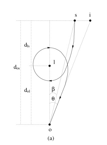
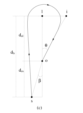
Figure 1: Schematic representation of the lens geometries. Case (a) corresponds to standard lensing, and cases (b) and (c) to retrolensing. The source (s), the lens (l), the observer (o) and the first relativistic image (i) are shown.

From the lens geometry it is easy to see that

$$b=d_{ol}\sin\theta,$$ (18)

which can be approximated to first order in $\theta$ by $b=d_{ol}\theta$, so the deflection angle given by Eq. (15) can be written as a function of $\theta$:

$$\alpha(\theta)=-c_{1}\ln\left(\frac{\theta}{\theta_{ps}}-1\right)+c_{2},$$ (19)

with $\theta_{ps}=2/d_{ol}$. Inverting Eq. (19) to obtain $\theta(\alpha)$

$$\theta(\alpha)=\theta_{ps}\left[1+e^{(c_{2}-\alpha)/c_{1}}\right],$$ (20)

and making a first order Taylor expansion around $\alpha=m\pi$, the angular position of the $m$-th image can be approximated by

$$\theta_{m}=\theta^{0}_{m}-\zeta_{m}\Delta\alpha_{m},$$ (21)

with

$$\theta^{0}_{m}=\theta_{ps}\left[1+e^{(c_{2}-m\pi)/c_{1}}\right],$$ (22)

and

$$\zeta_{m}=\frac{\theta_{ps}}{c_{1}}e^{(c_{2}-m\pi)/c_{1}}.$$ (23)

From Eq. (17)

$$\Delta\alpha_{m}=\frac{\theta_{m}-\beta}{c_{3}},$$ (24)

and replacing it in Eq. (21) leads to

$$\theta_{m}=\theta^{0}_{m}-\frac{\zeta_{m}}{c_{3}}(\theta_{m}-\beta),$$ (25)

which can be written in the form

$$\left(1+\frac{\zeta_{m}}{c_{3}}\right)\theta_{m}=\theta^{0}_{m}+\frac{\zeta_{m}}{c_{3}}\beta,$$ (26)

then

$$\theta_{m}=\left(1+\frac{\zeta_{m}}{c_{3}}\right)^{-1}\left(\theta^{0}_{m}+\frac{\zeta_{m}}{c_{3}}\beta\right),$$ (27)

which, using that $0<\zeta_{m}/c_{3}\ll 1$, can be approximated by

$$\theta_{m}=\left(1-\frac{\zeta_{m}}{c_{3}}\right)\left(\theta^{0}_{m}+\frac{\zeta_{m}}{c_{3}}\beta\right).$$ (28)

Then, keeping only the first order term in $\zeta_{m}/c_{3}$, the angular positions of the images are finally given by

$$\theta_{m}=\theta^{0}_{m}+\frac{\zeta_{m}}{c_{3}}(\beta-\theta^{0}_{m}).$$ (29)

The second term in Eq. (29) is a small correction on $\theta^{0}_{m}$, so all images lie very close to $\theta^{0}_{m}$. With a similar treatment, the other set of relativistic images have angular positions

$$\theta_{m}=-\theta^{0}_{m}+\frac{\zeta_{n}}{c_{3}}(\beta+\theta^{0}_{m}).$$ (30)

When $\beta=0$ an infinite sequence of Einstein rings is formed, with angular radius

$$\theta^{E}_{m}=\left(1-\frac{\zeta_{m}}{c_{3}}\right)\theta^{0}_{m}.$$ (31)

Since gravitational lensing conserves surface brightness [1], the ratio of the solid angles subtended by the image and the source gives the amplification of the $m$-th image:

$$\mu_{m}=\left|\frac{\sin\beta}{\sin\theta_{m}}\frac{d\beta}{d\theta_{m}}\right|^{-1}\approx\left|\frac{\beta}{\theta_{m}}\frac{d\beta}{d\theta_{m}}\right|^{-1},$$ (32)

so, using Eq. (29),

$$\mu_{m}=\frac{1}{\beta}\left[\theta^{0}_{m}+\frac{\zeta_{m}}{c_{3}}(\beta-\theta^{0}_{m})\right]\frac{\zeta_{m}}{c_{3}},$$ (33)

which can be approximated to first order in $\zeta_{m}/c_{3}$ by

$$\mu_{m}=\frac{1}{\beta}\frac{\theta^{0}_{m}\zeta_{m}}{c_{3}}.$$ (34)

The same result is obtained for the other set of images. The first relativistic image is the brightest one, and the magnifications decrease exponentially with $m$.

For standard lensing $m=2n$, and the total magnification, considering both sets of images, is $\mu=2\sum\limits_{n=1}^{\infty}\mu_{n}$, which using Eqs. (22), (23) and (34), leads to

$$\mu=\frac{1}{\beta}\frac{8}{d_{ol}^{2}c_{1}c_{3}}\frac{e^{c_{2}/c_{1}}\left(1+e^{c_{2}/c_{1}}+e^{2\pi/c_{1}}\right)}{e^{4\pi/c_{1}}-1}.$$ (35)

For retrolensing, $m=2n-1$, the total magnification, considering both sets of images, is

$$\mu=\frac{1}{\beta}\frac{8}{d_{ol}^{2}c_{1}c_{3}}\frac{e^{(c_{2}+\pi)/c_{1}}\left[1+e^{(c_{2}+\pi)/c_{1}}+e^{2\pi/c_{1}}\right]}{e^{4\pi/c_{1}}-1}.$$ (36)

Note that the amplifications of the strong field images are greater for retrolensing. In both cases, the magnifications are proportional to $1/d_{ol}^{2}$, which is a very small factor. Then, the relativistic images are very faint, unless $\beta$ has values close to zero, i.e. nearly perfect alignment. For $\beta=0$, the amplification becomes infinite, and the point source approximation breaks down, so an extended source analysis is necessary.

3.2 Extended source

For an extended source, it is necesary to integrate over its luminosity profile to obtain the magnification of the images:

$$\mu=\frac{\int\!\!\int_{S}\mathcal{I}\mu_{p}dS}{\int\!\!\int_{S}\mathcal{I}dS},$$ (37)

where $\mathcal{I}$ is the surface intensity distribution of the source and $\mu_{p}$ is the magnification corresponding to each point of the source. If the source is an uniform disk $D(\beta_{c},\beta_{s})$, with angular radius $\beta_{s}$ and centered in $\beta_{c}$ (taken positive), Eq. (37) can be put in the form

$$\mu=\frac{\int\!\!\int_{D(\beta_{c},\beta_{s})}\mu_{p}dS}{\pi\beta_{s}^{2}}.$$ (38)

Then, using Eq. (34), the magnification of the relativistic $m$-th image (with $m$ even for standard lensing and odd for retrolensing) for an extended uniform source is

$$\mu_{m}=\frac{I}{\pi\beta_{s}^{2}}\frac{\theta^{0}_{m}\zeta_{m}}{c_{3}},$$ (39)

with $I=\int\!\!\int_{D(\beta_{c},\beta_{s})}(1/\beta)dS$. This integral can be calculated in terms of elliptic integrals:

$$I=2\left[(\beta_{s}+\beta_{c})E\left(\frac{2\sqrt{\beta_{s}\beta_{c}}}{\beta_{s}+\beta_{c}}\right)+(\beta_{s}-\beta_{c})K\left(\frac{2\sqrt{\beta_{s}\beta_{c}}}{\beta_{s}+\beta_{c}}\right)\right],$$ (40)

where $K(k)$ and $E(k)$ are respectively, complete elliptic integrals of the first and second kind with argument $k=2\sqrt{\beta_{s}\beta_{c}}/(\beta_{s}+\beta_{c})$ [27]. Then the total amplification for standard lensing is

$$\mu=\frac{I}{\pi\beta_{s}^{2}}\frac{8}{d_{ol}^{2}c_{1}c_{3}}\frac{e^{c_{2}/c_{1}}\left(1+e^{c_{2}/c_{1}}+e^{2\pi/c_{1}}\right)}{e^{4\pi/c_{1}}-1},$$ (41)

and for retrolensing is

$$\mu=\frac{I}{\pi\beta_{s}^{2}}\frac{8}{d_{ol}^{2}c_{1}c_{3}}\frac{e^{(c_{2}+\pi)/c_{1}}\left[1+e^{(c_{2}+\pi)/c_{1}}+e^{2\pi/c_{1}}\right]}{e^{4\pi/c_{1}}-1}.$$ (42)

These expresions always give finite magnifications, even in the case of complete alignment.

4 Comparison with Schwarzschild black holes

The equations that give the positions and magnifications of the relativistic images obtained in Sec. 3 can be applied to the four dimensional Schwarzschild black hole, with the distances measured in units of the Schwarzschild radius $r_{H}^{Schw}=2(M/M_{4})l_{4}$, the photon sphere radius given by $r_{ps}^{Schw}=3r_{H}^{Schw}/2$, and the constants $c_{1}$ and $c_{2}$ replaced by $c_{1}^{Schw}=1$ and $c_{2}^{Schw}=\ln[216(7-4\sqrt{3})]-\pi$ [8] ($c_{3}$ does not change). The quotient between the $m$-th Einstein radius of the braneworld black hole and that of the Schwarzschild black hole with the same mass can be expressed in the form

$$\frac{\theta^{E}_{m}}{\theta^{E,Schw}_{m}}=\chi(m)\frac{c_{3}D_{ol}-32^{\sqrt{2}}2\sqrt{2}e^{-(m+1)\sqrt{2}\pi}r_{H}}{c_{3}D_{ol}-324(7-4\sqrt{3})e^{-(m+1)\pi}r_{H}^{Schw}}\left(\frac{l}{l_{4}}\right)^{1/2}\left(\frac{M}{M_{4}}\right)^{-1/2},$$ (43)

with $m$ even for standard lensing and odd for retrolensing, and

$$\chi(m)=\sqrt{\frac{32}{27\pi}}\frac{1+32^{\sqrt{2}}e^{-(m+1)\sqrt{2}\pi}}{1+216(7-4\sqrt{3})e^{-(m+1)\pi}}.$$ (44)

In the usual case when $c_{3}D_{ol}\gg 32^{\sqrt{2}}2\sqrt{2}r_{H}$ and $c_{3}D_{ol}\gg 324(7-4\sqrt{3})r_{H}^{Schw}$, Eq. (43) can be approximated by

$$\frac{\theta^{E}_{m}}{\theta^{E,Schw}_{m}}=\chi(m)\left(\frac{l}{l_{4}}\right)^{1/2}\left(\frac{M}{M_{4}}\right)^{-1/2}.$$ (45)

For the first Einstein radius, Eq. (44) gives $\chi\approx 0.6136$ for standard lensing, and $\chi\approx 0.6080$ for retrolensing. The quotient of the magnifications for the $m$-th image can be written as

$$\frac{\mu_{m}}{\mu^{Schw}_{m}}=\omega(m)\frac{l}{l_{4}}\frac{M_{4}}{M},$$ (46)

with

$$\omega(m)=\frac{32^{\sqrt{2}}4\sqrt{2}}{729(7-4\sqrt{3})\pi}\frac{\left[1+32^{\sqrt{2}}e^{-(m+1)\sqrt{2}\pi}\right]e^{-(m+1)(\sqrt{2}-1)\pi}}{1+216(7-4\sqrt{3})e^{-(m+1)\pi}},$$ (47)

which gives for the first image the values $\omega\approx 0.09318$ for standard lensing, and $\omega\approx 0.3392$ for retrolensing. The ratio of the total magnifications is

$$\frac{\mu}{\mu^{Schw}}=\kappa\frac{l}{l_{4}}\frac{M_{4}}{M},$$ (48)

with

$$\kappa=\frac{32^{\sqrt{2}}\sqrt{2}\left(e^{4\pi}-1\right)e^{-(\sqrt{2}-1)\pi}\left(1+32^{\sqrt{2}}e^{-\sqrt{2}\pi}+e^{2\sqrt{2}\pi}\right)}{324(7-4\sqrt{3})\left(e^{4\sqrt{2}\pi}-1\right)\left[1+216(7-4\sqrt{3})e^{-\pi}+e^{2\pi}\right]\pi}\approx 0.05232,$$ (49)

for standard lensing, and

$$\kappa=\frac{32^{\sqrt{2}}\sqrt{2}\left(e^{4\pi}-1\right)\left(1+32^{\sqrt{2}}+e^{2\sqrt{2}\pi}\right)}{324(7-4\sqrt{3})\left(e^{4\sqrt{2}\pi}-1\right)\left[1+216(7-4\sqrt{3})+e^{2\pi}\right]\pi}\approx 0.1905,$$ (50)

for retrolensing.

The quotient of the Einstein radii is roughly proportional to $r_{H}/r^{Schw}_{H}\propto(l/M)^{1/2}$, whereas the ratio of the amplifications is proportional to $(r_{H}/r^{Schw}_{H})^{2}\propto l/M$. Note that even in the case of a braneworld black hole and a Schwarzschild black hole with the same mass and the same horizon event radius, the Einstein radii and magnifications are different. As in the weak field lensing case [24], the strong field images for the braneworld black hole increase their brightness with respect to the Schwarzschild black hole for larger values of the extra dimension $l$.

5 Conclusions

In this work, the positions and magnifications of the relativistic images were calculated, using the strong field limit, for a braneworld black hole. These black holes were previously studied as primordial black holes [22, 23], and can be relics of a past high energy phase of the Universe. They have a larger size, are colder, and live longer than their four dimensional Schwarzschild counterpart of the same mass [20]. Current experiments that test the gravitational inverse square law, lead to an upper limit for the extra dimension given by $l\leq 0.1$ mm [28]. The condition that the event horizon radius $r_{H}$ is much smaller than the Ads radius $l$ for the braneworld black holes studied in this paper, means that these black holes, if they exist, are very small. The astronomical observation of the relativistic images is a difficult task that is beyond current technologies, and it will be a challenge for the next generation of instruments in the case of more massive black holes [17]. The observation seems even more difficult in the case of the small size braneworld black holes analyzed in this paper. But there could be another route for seeing the strong field lensing effects for these low mass black holes. The presence of the extra dimension dramatically decreases the energy necessary to produce black holes by particle collisions [20, 29]. Only energies of about $1$ TeV are needed instead of energy scales about $10^{16}$ TeV required if no extra dimensions are present. These small size black holes could be created in the next generation particle accelerators or detected in cosmic rays [20, 29]. With these black holes acting as gravitational lenses, the order of magnitude of the distances involved would be meters or less, instead of kilo-parsecs, so that the angular positions and magnifications obtained in Sec. 3 will be considerably larger than in the astronomical case corresponding to black holes with the same mass . If the extra dimensions hypothesis is correct, it will open up the exciting possibility that the interesting phenomena of strong field lensing can be observed in the laboratory in future times.

References

- [1] P. Schneider, J. Ehlers, and E.E. Falco, Gravitational Lenses (Springer-Verlag, Berlin, 1992).
- [2] K.S. Virbhadra, and G.F.R. Ellis, Phys. Rev. D 62, 084003 (2000).
- [3] K.S. Virbhadra, and G.F.R. Ellis, Phys. Rev. D 65, 103004 (2002).
- [4] S. Frittelli, T.P. Kling, and E.T. Newman, Phys. Rev. D 61, 064021 (2000).
- [5] C. Darwin, Proc. Roy. Soc London A 249, 180 (1959); J.-P. Luminet, Astron. Astrophys. 75, 228 (1979); S. Chandrasekhar, The Mathematical Theory of Black Holes (Oxford University Press, Oxford, 1983); H.C. Ohanian, Am. J. Phys. 55, 428 (1987).
- [6] V. Bozza, S. Capozziello, G. Iovane, and G. Scarpetta, Gen. Relativ. Gravit. 33, 1535 (2001).
- [7] E.F. Eiroa, G.E. Romero, and D.F. Torres, Phys. Rev. D 66, 024010 (2002).
- [8] V. Bozza, Phys. Rev. D 66, 103001 (2002).
- [9] A. Bhadra, Phys. Rev. D 67, 103009 (2003).
- [10] A.O. Petters, Mon. Not. R. Astron. Soc. 338, 457 (2003).
- [11] V. Bozza, and L. Mancini, Gen. Relativ. Gravit. 36, 435 (2004).
- [12] V. Bozza, Phys. Rev. D 67, 103006 (2003).
- [13] D.E. Holtz and J.A. Wheeler, Astrophys. J. 578, 330 (2002).
- [14] F. De Paolis, A. Geralico, G. Ingrosso, and A.A. Nucita, Astron. Astrophys. 409, 809 (2003).
- [15] E.F. Eiroa and D.F. Torres, Phys. Rev. D 69, 063004 (2004).
- [16] F. De Paolis, A. Geralico, G. Ingrosso, A.A. Nucita, and A. Qadir, Astron. Astrophys. 415, 1 (2004).
- [17] V. Bozza and L. Mancini, Astrophys. J. 611, 1045 (2004).
- [18] R.J. Nemiroff, Am. J. Phys. 61, 619 (1993); S. Frittelli and E.T. Newman, Phys. Rev. D 59, 124001 (1999); M.P. Dabrowski and F.E. Schunck, Astrophys. J. 535, 316 (2000); C.M. Claudel, K.S. Virbhadra, and G.F.R. Ellis, J. Math. Phys. 42, 818 (2001); V. Perlick, Commun. Math. Phys. 220, 403 (2001); S. Frittelli and E.T. Newman, Phys. Rev. D 65, 123006 (2002); S. Frittelli, T.P. Kling, and E.T. Newman, Phys. Rev. D 65, 123007 (2002); V. Perlick, Phys. Rev. D 69, 064017 (2004).
- [19] D. Langlois, Prog. Theor. Phys. Suppl. 148, 181 (2002); P. Brax and C. van de Bruck, Class. Quantum Grav. 20, R201 (2003); R. Maartens, Living Rev. Relativity 7, 7 (2004).
- [20] P. Kanti, Int. J. Mod. Phys. A 19, 4899 (2004).
- [21] L. Randall and R. Sundrum, Phys. Rev. Lett. 83, 3370 (1999); L. Randall and R. Sundrum, Phys. Rev. Lett. 83, 4690 (1999).
- [22] R. Guedens, D. Clancy, and A.R. Liddle, Phys. Rev. D 66, 043513 (2002); R. Guedens, D. Clancy, and A.R. Liddle, Phys. Rev. D 66, 083509 (2002); D. Clancy, R. Guedens, and A.R. Liddle, Phys. Rev. D 68, 023507 (2003).
- [23] A.S. Majumdar, Phys. Rev. Lett. 90, 031303 (2003).
- [24] A.S. Majumdar and N. Mukherjee, arXiv:astro-ph/0403405 (2004).
- [25] V. Frolov, M. Snajdr, and D. Stojkovic, Phys. Rev. D 68, 044002 (2003).
- [26] S. Weinberg, Gravitation and Cosmology: Principles and Applications of the General Theory of Relativity (Wiley, New York, 1972).
- [27] I.S. Gradshteyn and I.M. Ryzhik, Table of Integrals, Series and Products, 5th ed., edited by A. Jeffrey (Academic Press, San Diego, 1994).
- [28] J.C. Long, H.W. Chan, A.B. Churnside, E.A. Gulbis, M.C.M. Varney, and J.C. Price, Nature 421, 922 (2003).
- [29] S.B. Giddings, Gen. Relativ. Gravit. 34, 1775 (2002); M. Cavaglia, Int. J. Mod. Phys. A 18, 1843 (2003).