The gravitational self-force

Abstract

The self-force describes the effect of a particle’s own gravitational field on its motion. While the motion is geodesic in the test-mass limit, it is accelerated to first order in the particle’s mass. In this contribution I review the foundations of the self-force, and show how the motion of a small black hole can be determined by matched asymptotic expansions of a perturbed metric. I next consider the case of a point mass, and show that while the retarded field is singular on the world line, it can be unambiguously decomposed into a singular piece that exerts no force, and a smooth remainder that is responsible for the acceleration. I also describe the recent efforts, by a number of workers, to compute the self-force in the case of a small body moving in the field of a much more massive black hole.

The motivation for this work is provided in part by the Laser Interferometer Space Antenna, which will be sensitive to low-frequency gravitational waves. Among the sources for this detector is the motion of small compact objects around massive (galactic) black holes. To calculate the waves emitted by such systems requires a detailed understanding of the motion, beyond the test-mass approximation.

This article is based on a plenary lecture presented at the 17th International Conference on General Relativity and Gravitation, which took place in July, 2004 in Dublin, Ireland.

I Introduction: The Capra scientific mandate

This contribution describes how a body of mass $m$, supposed to be “small”, moves in spacetime. In the test-mass approximation it is known that the body moves on a geodesic of a background spacetime whose metric $g_{\alpha\beta}$ does not depend on $m$. As $m$ increases (but kept small) the test-mass description is no longer adequate. One might then say that the motion is still geodesic, but in a spacetime whose metric is perturbed with respect to the background metric. Alternatively, one might say that the motion is accelerated in the background spacetime. This is the point of view I shall take in this contribution: The body’s motion will be described in the original (unperturbed) spacetime, and the gravitational influence of the body will be incorporated in its acceleration. The body will be said to move under the influence of its gravitational self-force.

The work described here was previously reviewed in a very long article published in Living Reviews in Relativity poisson:04b . An abridged version of this article appeared in Classical and Quantum Gravity poisson:04c . This contribution focuses on the highlights and presents the “big picture”. The reader is warned that my presentation will be sketchy and incomplete, and is referred to the review articles for additional details. The scientific objectives behind the work described here have been pursued by a number of people; I like to refer to these objectives as the “Capra scientific mandate” and to these people as the “Capra posse”.

The Capra scientific mandate includes three main objectives. The first is to formulate the equations of motion of a small body in a specified background spacetime, beyond the test-mass approximation. This first step was solved in 1997, first by Mino, Sasaki, and Tanaka mino-etal:97 , and then by Quinn and Wald quinn-wald:97 . The equations of motion are now known as the MiSaTaQuWa equations; I will sketch their derivation in this contribution. The second objective is to concretely describe the motion of the small body in situations of astrophysical interest, including generic orbits of a Kerr black hole. There has been much recent progress on this front, and I will describe some of the issues involved in this contribution. The third objective is to properly incorporate the equations of motion into a wave-generation formalism. This final objective is the most important, as the ultimate goal of this enterprise is to make detailed predictions toward eventual gravitational-wave measurements. This is the holy grail of the Capra program, and it has so far proved elusive. I will present a tentative outline of future work in the last section of this contribution.

The work reviewed in this contribution was shaped by a series of annual meetings named after the late movie director Frank Capra. The first of these meetings took place in 1998 and was held at Capra’s ranch in Southern California; the ranch now belongs to Caltech, Capra’s alma mater. Subsequent meetings were held in Dublin, Pasadena, Potsdam, State College PA, Kyoto, and Brownsville.

Members of the Capra posse include Paul Anderson, Warren Anderson, Leor Barack, Patrick Brady, Lior Burko, Manuella Campanelli, Steve Detweiler, Eanna Flanagan, Costas Glempedakis, Abraham Harte, Wataru Hikida, Bei Lok Hu, Scott Hughes, Sanjay Jhingan, Dong-Hoon Kim, Carlos Lousto, Eirini Messaritaki, Yasushi Mino, Hiroyuki Nakano, Amos Ori, Ted Quinn, Eran Rosenthal, Norichika Sago, Misao Sasaki, Takahiro Tanaka, Bob Wald, Bernard Whiting, and Alan Wiseman.

II Astrophysical context

The motivation for the Capra program comes largely from the fact that solar-mass compact bodies moving around massive black holes have been identified as one of the promising sources of gravitational waves for the space-based interferometric detector LISA (Laser Interferometer Space Antenna). (The case for this identification is made in the contributions by Sterl Phinney and Sir Martin Rees.) These systems involve highly eccentric, nonequatorial, and relativistic orbits around rapidly rotating black holes. The waves produced by these orbits will be rich in information concerning the strongest gravitational fields in the Universe, and this information will be extractable from the LISA data stream. The extraction, however, will depend on sophisticated data-analysis strategies that will rely on a detailed and accurate modeling of the source. This modeling involves formulating the equations of motion for the small body in the field of the rotating black hole, in a small-mass-ratio approximation that goes beyond the test-mass description. And it involves a consistent incorporation of these equations of motion into a wave-generation formalism. In short, the extraction of this wealth of information relies on the successful completion of the Capra program.

The finite-mass corrections to the orbiting body’s motion are important. Let $m$ be the mass of the orbiting body, $M$ the mass of the central black hole, and suppose that $m/M\ll 1$. For concreteness, assume that the orbiting body is a $10\ M_{\odot}$ black hole and that the central black hole has a mass of $10^{6}\ M_{\odot}$. Then $m/M=10^{-5}$ is the order of magnitude of the correction to the equations of motion relative to the test-mass description. Simultaneously, $M/m=10^{5}$ is the order of magnitude of the total number of wave cycles that will be received during a year’s worth of LISA observation. This simplistic estimate illustrates that while the corrections to the equations of motion are small, in the course of a year they can accumulate and contribute a significant number of wave cycles.

Corrections to the equations of motion must incorporate both conservative and dissipative effects. Finite-mass corrections that are conservative in nature are familiar from Newtonian and post-Newtonian theory, and they occur also in a strong-gravity situation. These can accumulate over time. Imagine, for example, an eccentric orbit that undergoes periastron advance. A finite-mass correction to this effect will cause a steady drift in the phasing of the orbit, and this will directly be reflected in the phasing of the gravitational waves; after $10^{5}$ orbital cycles the $10^{-5}$ correction will have grown into a sizable effect.

Dissipative effects, on the other hand, do not occur in Newtonian gravity, but they are familiar in post-Newtonian theory; they are also present in a strong-gravity situation. Dissipation is associated with the radiative loss of energy and angular momentum by the orbital system, and the resulting corrections to the motion also accumulate over time; this translates into a steady drift of the gravitational-wave signal in the LISA frequency band. These are finite-mass corrections, because the test-mass description makes no room for gravitational radiation and radiation reaction.

From a more theoretical point of view, the appeal of this work comes largely from the fact that while the motion of self-gravitating bodies has been studied extensively in the context of post-Newtonian theory (see, for example, Refs. damour:87 ; blanchet:02 ), very little is known in the case of strong fields and fast motions. To the relativist working in this area, this problem is irresistible: We have strong gravity, fast motion, and a smallness parameter in the form of $m/M$. We have a cool problem that can be solved by standard perturbative techniques.

III Motion of a black hole

Let me restate the problem in its most general form: A body of mass $m$ moves in an arbitrary (but empty of matter) spacetime whose radius of curvature (in the body’s neighbourhood) is ${\cal R}$; what is the description of its motion when $m\ll{\cal R}$? This formulation of the problem is more general than the two-body version stated previously. When the small body is a member of a binary system, and is at a distance $b$ from another body of mass $M$, then ${\cal R}\sim\sqrt{b^{3}/(M+m)}$ and

$$\frac{m}{{\cal R}}\sim\frac{m}{M+m}v^{3},$$

where $v=\sqrt{(M+m)/b}$. For relativistic motion ($v\sim 1$) this is small whenever $m/M\ll 1$.

The clean separation of scales allows us to idealize the motion as following a world line in a spacetime whose metric $g_{\alpha\beta}$ will be specified below. While the region of spacetime occupied by the body is truly a world tube of finite extension, on a scale ${\cal R}$ — the only scale of relevance in the background spacetime — this extension is so small that little is lost by making this idealization. The body shall then follow a world line $\gamma$ that will be described by parametric relations $z^{\mu}(\tau)$, in which $\tau$ is proper time measured in the metric $g_{\alpha\beta}$. We wish to determine this world line. It is understood that the world line loses all significance when the neighbourhood of the body is examined on the fine scale $m$; on this scale the finite extension of the world tube is fully revealed.

It is desirable to choose the body to have an internal structure that is as simple as possible. One thus eliminates an important source of technical complications, but one still feels confident that the resulting equations of motion will apply, to a good degree of accuracy, to a body of arbitrary structure. (This “effacement property” of the internal structure is well established in post-Newtonian theory damour:87 .) This attitude often leads the researcher to assume that the body is a point particle. We shall refrain from doing so at this stage, but we will come back to this description in Sec. IV. We shall instead choose the body to have the simplest structure compatible with the laws of general relativity: it shall be a nonrotating black hole. This was one of the starting assumptions of Mino, Sasaki, and Tanaka mino-etal:97 (see also Ref. poisson:04a ).

The motion of the black hole is determined by matched asymptotic expansions, a powerful technique that has known many useful applications in general relativity (see, for example, Refs. thorne-hartle:85 ; death:96 ). In this approach the metric of the black hole perturbed by the tidal gravitational field supplied by the external universe is matched to the metric of the external universe perturbed by the moving black hole. Demanding that this metric be a valid solution to the Einstein field equations determines the motion without additional input.

The method of matched asymptotic expansions relies on the existence of (i) an internal zone in which gravity is dominated by the black hole, (ii) an external zone in which gravity is dominated by the conditions in the external universe, and (iii) an overlapping region known as the buffer zone, in which the black hole and the external universe have comparable influence. Let $r$ be a meaningful measure of spatial distance from the black hole. Then the internal zone is the region of spacetime in which $r<r_{i}=\mbox{constant}$, where $r_{i}\ll{\cal R}$; thus $r/{\cal R}$ is small throughout the internal zone and the tidal influence of the external universe is small. The external zone, on the other hand, is the region of spacetime in which $r>r_{e}=\mbox{constant}$, where $r_{e}\gg m$; thus $m/r$ is small throughout the external zone and the gravitational effects of the black hole are small. Finally, the buffer zone is the region of spacetime in which $r_{e}<r<r_{i}$. This region exists because $m\ll{\cal R}$, and $r/{\cal R}$ and $m/r$ are simultaneously small in the buffer zone.

An expansion of the metric in the internal zone has the schematic form

$${\sf g}=g(\mbox{Schwarzschild})+O(r^{2}/{\cal R}^{2})+\cdots,$$ (1)

where $g(\mbox{Schwarzschild})$ is the metric of a nonrotating black hole in isolation, and $O(r^{2}/{\cal R}^{2})$ is the tidal field supplied by the external universe. (Terms that scale as $r/{\cal R}$ have been removed by a coordinate transformation.) On the other hand, an expansion of the metric in the external zone has the schematic form

$${\sf g}=g(\mbox{background})+O(m/r)+\cdots,$$ (2)

where $g(\mbox{background})$ is the metric of the external universe in the absence of the black hole, and $O(m/r)$ is the perturbation produced by the moving black hole. The key idea of matched asymptotic expansions is that the expansions of Eqs. (1) and (2) are both valid in the buffer zone, and that both forms of ${\sf g}$ represent the same metric (up to a coordinate transformation). Performing the matching returns the black hole’s equations of motion.

External zone

To flesh out these ideas let us first examine the situation in the external zone. Let $g_{\alpha\beta}$ stand for $g(\mbox{background})$, the metric of the external universe in the absence of the small black hole. (In the astrophysical context of Sec. II this would be the metric of the massive black hole, in isolation.) Let $\gamma$ be a fiducial world line in this background spacetime (later to be identified with the small hole’s world line), and express the metric in normal coordinates centered on $\gamma$. It will have the form of $g=\eta+O(r/{\cal R})+O(r^{2}/{\cal R}^{2})+\cdots$, where $\eta$ is the metric of flat spacetime. The normal coordinates do not extend beyond $r={\cal R}$ and are therefore restricted to the buffer zone.

More specifically, let the normal coordinates be the retarded coordinates $(u,x^{a}=r\Omega^{a})$, such that $u$ is constant on each future light cone centered on $\gamma$ (and $u$ is equal to proper time on the world line), $r$ is an affine parameter on the cone’s null generators, and $\Omega^{a}\equiv x^{a}/r$ is constant on each generator. Then the time-time component of the background metric takes the form

$$g_{uu}=-\bigl{(}1+2ra_{a}\Omega^{a}+r^{2}{\cal E}_{ab}\Omega^{a}\Omega^{b}\bigr{)}+O(r^{3}/{\cal R}^{3}),$$ (3)

where $a_{a}(u)$ is the acceleration vector of the world line, and ${\cal E}_{ab}(u)=C_{uaub}=O(1/{\cal R}^{2})$ are the electric components of the Weyl tensor evaluated on $\gamma$. (This three-tensor is symmetric and tracefree.) Our main goal is to eventually determine $a_{a}$; we can anticipate that $a_{a}=O(m/{\cal R}^{2})$ since the motion must be geodesic in the test-mass limit.

Let $h_{\alpha\beta}$ be the perturbation produced by the moving black hole, so that the full metric is ${\sf g}_{\alpha\beta}=g_{\alpha\beta}+h_{\alpha\beta}$. A standard technique in perturbation theory is to introduce the trace-reversed potentials

$$\psi_{\alpha\beta}=h_{\alpha\beta}-\frac{1}{2}g_{\alpha\beta}\bigl{(}g^{\gamma\delta}h_{\gamma\delta}\bigr{)}$$ (4)

and to impose the Lorenz gauge condition

$$\psi^{\alpha\beta}_{\ \ \ ;\beta}=0.$$ (5)

Here and below, all indices are manipulated with the background metric, and covariant differentiation is taken to be compatible with this metric.

In the external zone the perturbation produced by the black hole cannot be distinguished from one produced by a point particle of mass $m$ moving on $\gamma$, and $\psi_{\alpha\beta}$ must be a solution to the wave equation

$$\Box\psi^{\alpha\beta}+2R^{\alpha\ \beta}_{\ \gamma\ \delta}\psi^{\gamma\delta}=-16\pi T^{\alpha\beta},$$ (6)

where $T^{\alpha\beta}$ is the particle’s stress-energy tensor. This equation can be solved by means of a retarded Green’s function,

$$G^{\alpha\beta}_{\ \ \gamma^{\prime}\delta^{\prime}}(x,x^{\prime})=U^{\alpha\beta}_{\ \ \gamma^{\prime}\delta^{\prime}}(x,x^{\prime})\delta(\sigma)+V^{\alpha\beta}_{\ \ \gamma^{\prime}\delta^{\prime}}(x,x^{\prime})\theta(-\sigma),$$ (7)

where $\sigma(x,x^{\prime})$ is half the squared geodesic distance between the points $x$ and $x^{\prime}$, and $U^{\alpha\beta}_{\ \ \gamma^{\prime}\delta^{\prime}}(x,x^{\prime})$, $V^{\alpha\beta}_{\ \ \gamma^{\prime}\delta^{\prime}}(x,x^{\prime})$ are smooth bitensors. The Green’s function is decomposed into a singular “light-cone part” that has support on $\sigma=0$ only, and a smooth “tail part” that has support on $\sigma<0$ (so that $x$ is in the chronological future of $x^{\prime}$). (It should be noted that this representation of the Green’s function is valid only when $x$ is in the normal convex neighbourhood of $x^{\prime}$. In the sequel I will simplify expressions by pretending that the decomposition holds globally. The reader is referred to LRR poisson:04b for all the fine print.)

The solution to Eq. (6) is

$$\psi^{\alpha\beta}(x)=\frac{4m}{r}U^{\alpha\beta}_{\ \ \gamma^{\prime}\delta^{\prime}}(x,x^{\prime})u^{\gamma^{\prime}}u^{\delta^{\prime}}+\psi^{\alpha\beta}_{\rm tail}(x)$$ (8)

where $x^{\prime}\equiv z^{\mu}(u)$ is the point on the world line that is linked to $x$ by a null geodesic, $u$ the value of the proper-time parameter at this retarded point, $u^{\gamma^{\prime}}$ the four-velocity at the retarded point, and

$$\psi^{\alpha\beta}_{\rm tail}(x)=4m\int_{-\infty}^{u}V^{\alpha\beta}_{\ \ \mu^{\prime}\nu^{\prime}}(x,z^{\prime})u^{\mu^{\prime}}u^{\nu^{\prime}}\,d\tau^{\prime}$$ (9)

is the “tail” term. Here $z^{\prime}\equiv z(\tau^{\prime})$ stands for an arbitrary position on the world line, and the potentials of Eq. (8) depend on the particle’s entire history prior to the retarded point $\tau=u(x)$.

Inverting Eq. (4) and expressing the results in the retarded coordinates $(u,r\Omega^{a})$ returns

$${\sf g}_{uu} = -1-r^{2}{\cal E}_{ab}\Omega^{a}\Omega^{b}+O(r^{3}/{\cal R}^{3})$$ (10)

$$\mbox{}+\frac{2m}{r}+h^{\rm tail}_{uu}+r\bigl{(}2m{\cal E}_{ab}\Omega^{a}\Omega^{b}-2a_{a}\Omega^{a}$$

$$\mbox{}+h^{\rm tail}_{uuu}+h^{\rm tail}_{uua}\Omega^{a}\bigr{)}+O(mr^{2}/{\cal R}^{3})$$

for the time-time component of the perturbed metric ${\sf g}_{\alpha\beta}=g_{\alpha\beta}+h_{\alpha\beta}$. The fields $h^{\rm tail}_{\alpha\beta}$ are obtained from $\psi^{\rm tail}_{\alpha\beta}$ by trace reversal, and $h^{\rm tail}_{\alpha\beta\gamma}=\nabla_{\gamma}h^{\rm tail}_{\alpha\beta}$.

Equation (10) gives the metric of the external universe perturbed by a black hole moving on a world line $\gamma$ with an (as yet undetermined) acceleration $a_{a}(u)$. It is noteworthy that this metric appears to be singular when $r\to 0$. The metric, however, is valid only in the external zone $r>r_{e}\gg m$, and the limit $r\to 0$ is unattainable. The world line $\gamma$ is outside the metric’s domain of validity.

Internal zone

To obtain the metric of a nonrotating black hole that is slightly distorted by a tidal gravitational field is a standard application of black-hole perturbation theory. To leading order in the perturbation, which scales as $1/{\cal R}^{2}$, it is sufficient to integrate a set of time-independent perturbation equations, because each time derivative comes with an extra factor of $1/{\cal R}$, the inverse time scale associated with changes in the external universe. The perturbation must be well behaved on the hole’s event horizon, and the asymptotic conditions for $r\gg 2m$ are such that the perturbation must behave as $-r^{2}{\cal E}_{ab}\Omega^{a}\Omega^{b}$, which has a quadrupolar form. These observations make solving the perturbation equations a very straightforward task.

In a set of internal light-cone coordinates $(\bar{u},\bar{x}^{a}=\bar{r}\bar{\Omega}^{a})$ the time-time component of the perturbed metric reads

$${\sf g}_{\bar{u}\bar{u}}=-f-\bar{r}^{2}f^{2}{\cal E}_{ab}\bar{\Omega}^{a}\bar{\Omega}^{b}+O(\bar{r}^{3}/{\cal R}^{3}),$$ (11)

where $f=1-2m/\bar{r}$ and ${\cal E}_{ab}(\bar{u})$ is the tidal gravitational field supplied by the external universe. In the limit $m/\bar{r}\to 0$ (keeping $\bar{r}/{\cal R}$ fixed) Eq. (11) becomes the metric of the external universe, expressed in coordinates for which $a_{a}=0$. In the limit $\bar{r}/{\cal R}\to 0$ (keeping $m/\bar{r}$ fixed) Eq. (11) becomes the metric of a Schwarzschild black hole expressed in Eddington-Finkelstein coordinates. For small values of $\bar{r}/{\cal R}$ and arbitrary values of $m/\bar{r}$ Eq. (11) describes a tidally distorted black hole. The metric of Eq. (11) is valid everywhere in the internal zone, where $r<r_{i}\ll{\cal R}$.

Matching

Equation (10) gives the spacetime metric in the external zone, and the requirement that $r/{\cal R}\ll 1$ implies that the metric is in fact restricted to the buffer zone. Equation (11), on the other hand, gives the spacetime metric in the internal zone, and its specialization to $m/\bar{r}\ll 1$ implies also a restriction to the buffer zone. Since both metrics describe the geometry of the same region of the same spacetime, they must be related by a coordinate transformation.

The transformation from the external coordinates $(u,x^{a})$ to the internal coordinates $(\bar{u},\bar{x}^{a})$ is given in part by

$$\bar{u} = u-2m\ln r-\frac{1}{2}\int^{u}h^{\rm tail}_{uu}\,du-\frac{1}{2}r\Bigl{[}h^{\rm tail}_{uu}+2h^{\rm tail}_{ua}\Omega^{a}$$ (12)

$$\mbox{}+h^{\rm tail}_{ab}\Omega^{a}\Omega^{b}\Bigr{]}-\frac{1}{4}r^{2}\Bigl{[}h^{\rm tail}_{uuu}+\bigl{(}h^{\rm tail}_{uua}+2h^{\rm tail}_{uau}\bigr{)}\Omega^{a}$$

$$\mbox{}+\bigl{(}h^{\rm tail}_{abu}+2h^{\rm tail}_{uab}\bigr{)}\Omega^{a}\Omega^{b}+h^{\rm tail}_{abc}\Omega^{a}\Omega^{b}\Omega^{c}\Bigr{]}$$

$$\mbox{}+O(mr^{3}/{\cal R}^{3}).$$

Applying this transformation to Eq. (10) gives

$${\sf g}_{\bar{u}\bar{u}} = -1-\bar{r}^{2}{\cal E}_{ab}\bar{\Omega}^{a}\bar{\Omega}^{b}+O(\bar{r}^{3}/{\cal R}^{3})$$ (13)

$$\mbox{}+\frac{2m}{\bar{r}}+4m\bar{r}{\cal E}_{ab}\bar{\Omega}^{a}\bar{\Omega}^{b}$$

$$\mbox{}-2\bar{r}\biggl{(}a_{a}-\frac{1}{2}h^{\rm tail}_{uua}+h^{\rm tail}_{uau}\biggr{)}\bar{\Omega}^{a}$$

$$\mbox{}+O(m\bar{r}^{2}/{\cal R}^{3}).$$

Comparison with Eq. (11) — linearized with respect to $m/\bar{r}$ — reveals that the acceleration vector must be given by

$$a_{a}=\frac{1}{2}h^{\rm tail}_{uua}-h^{\rm tail}_{uau}.$$ (14)

As expected, the matching of the perturbed metrics in the buffer zone has returned the black hole’s equations of motion.

MiSaTaQuWa equations

The tensorial form of Eq. (14) is

$$\frac{Du^{\mu}}{d\tau}=-\frac{1}{2}\bigl{(}g^{\mu\nu}+u^{\mu}u^{\nu}\bigr{)}\bigl{(}2h^{\rm tail}_{\nu\lambda\rho}-h^{\rm tail}_{\lambda\rho\nu}\bigr{)}u^{\lambda}u^{\rho},$$ (15)

and these are the MiSaTaQuWa equations of motion. Here, $z^{\mu}(\tau)$ gives the description of the black hole’s motion in the background spacetime, $u^{\mu}=dz^{\mu}/d\tau$ is the normalized velocity vector, and $Du^{\mu}/d\tau$ is the covariant acceleration. All tensors, and all tensorial operations, refer to the background spacetime of the external universe; its metric is $g_{\alpha\beta}$, as it was introduced in Eq. (2).

The tail field on the right-hand side of Eq. (15) is obtained by differentiating Eq. (9); when expressed in terms of the original retarded Green’s function of Eq. (7) it is given by

$$h^{\rm tail}_{\mu\nu\lambda} = 4m\int_{-\infty}^{\tau-\epsilon}\nabla_{\lambda}\biggl{(}G_{\mu\nu\mu^{\prime}\nu^{\prime}}-\frac{1}{2}g_{\mu\nu}G^{\rho}_{\ \rho\mu^{\prime}\nu^{\prime}}\biggr{)}(z,z^{\prime})$$ (16)

$$\mbox{}\times u^{\mu^{\prime}}u^{\nu^{\prime}}\,d\tau^{\prime}.$$

It is understood that one takes the limit $\epsilon\to 0^{+}$ of this expression. Cutting the integration short excludes the (singular) light-cone part of the Green’s function and isolates its tail part; the result is a smooth field on the world line. In Eq. (16), $z\equiv z(\tau)$ stands for the current position on the world line (at which the self-force is being evaluated) and $z^{\prime}\equiv z(\tau^{\prime})$ stands for a prior position.

IV Motion of a point mass

The derivation of the MiSaTaQuWa equations sketched in the preceding section is conceptually sound and devoid of any questionable assumptions. It is, however, technically involved and one wonders whether there may not be a shortcut to the final answer. Since the equations of motion refer to a body without internal structure, could they be derived on the assumption that the object is a point particle? The answer is in the affirmative, provided that one is willing to introduce additional assumptions and tolerate fields that are singular on the world line. The derivation sketched below was first presented by Mino, Tanaka, and Sasaki mino-etal:97 and then by Quinn and Wald quinn-wald:97 ; the approach described here relies heavily on concepts and techniques introduced by Detweiler and Whiting detweiler-whiting:03 .

As we have seen in Sec. III, the gravitational perturbation produced by a point particle of mass $m$ is obtained from the potentials of Eq. (8) by trace reversal: $h_{\alpha\beta}=\psi_{\alpha\beta}-\frac{1}{2}g_{\alpha\beta}(g^{\gamma\delta}\psi_{\gamma\delta})$. In Sec. III, Eq. (8) was assumed to hold in the external zone only ($r>r_{e}\gg m$), but we now accept its global validity. We also accept the fact that the perturbation is singular on the world line ($r=0$). And we choose not to be bothered with the fact that while Eq. (8) was obtained by linearizing the Einstein field equations about the background metric $g_{\alpha\beta}$, the perturbation is obviously not small when $r$ is smaller than $m$.

Our first additional assumption is that the particle will move on a geodesic of the metric ${\sf g}_{\alpha\beta}=g_{\alpha\beta}+h_{\alpha\beta}$. Writing down the geodesic equation in terms of tensorial quantities that refer to the background spacetime (such as the velocity vector $u^{\mu}=dz^{\mu}/d\tau$, which is normalized in the metric $g_{\alpha\beta}$) returns the equations of motion

$$\frac{Du^{\mu}}{d\tau}=-\frac{1}{2}\bigl{(}g^{\mu\nu}+u^{\mu}u^{\nu}\bigr{)}\bigl{(}2h_{\nu\lambda;\rho}-h_{\lambda\rho;\nu}\bigr{)}u^{\lambda}u^{\rho}.$$ (17)

These are superficially similar to Eq. (15), but the difference is important. While Eq. (15) involves tensor fields that are smooth on the world line, Eq. (17) involves highly singular quantities. These equations of motion are therefore meaningless as they stand, and $h_{\alpha\beta}$ must be regularized before Eq. (17) can be evaluated.

The regularization of a retarded field near its pointlike source is a problem that has a long history. This issue was encountered by Dirac dirac:38 in the context of the electrodynamics of a point electric charge in flat spacetime. By appealing to energy-momentum conservation across a world tube surrounding the charge’s world line, Dirac discovered that regularization could be achieved by decomposing the electromagnetic field into singular-symmetric “S” and regular-radiative “R” pieces; the “S” field would simply be removed from the retarded field and only the remainder — the “R” field — would be allowed to act on the particle. Dirac further discovered that in flat spacetime, the “S” field is given by the following combination of retarded and advanced solutions to Maxwell’s equations: $F^{\rm S}_{\alpha\beta}=\frac{1}{2}(F^{\rm ret}_{\alpha\beta}+F^{\rm adv}_{\alpha\beta})$. The “R” field, on the other hand, is given by $F^{\rm R}_{\alpha\beta}=\frac{1}{2}(F^{\rm ret}_{\alpha\beta}-F^{\rm adv}_{\alpha\beta})$. Because the “S” field satisfies the same field equations as the retarded field (with a singular source term on the right-hand side), it is just as singular as the retarded field on the world line; removing it from the retarded field produces a smooth field. This is confirmed by the fact that the “R” field satisfies the sourcefree Maxwell equations.

Dirac’s analysis was generalized to curved spacetime by DeWitt and Brehme dewitt-brehme:60 , but the proper decomposition of the retarded electromagnetic field into “S” and “R” parts was identified only recently by Detweiler and Whiting detweiler-whiting:03 . For reasons of causality, the flat-spacetime prescription (a superposition of half retarded and half advanced fields) does not work in curved spacetime: The retarded field depends on the particle’s entire past history, the advanced field depends on its future history, and a linear superposition would depend on the full history, both past and future (see Fig. 1). This would give rise to equations of motion with unacceptable causal properties.

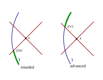
Figure 1: Causal properties of the retarded and advanced solutions. The retarded field at a point $x$ depends on the particle’s history prior to (and including) the retarded point $z(u)$. The advanced solution depends on the particle’s history after (and including) the advanced point $z(v)$.

The correct curved-spacetime prescription (identified by Detweiler and Whiting, and applied to the gravitational case) is to remove the “S” potential

$$\psi_{\rm S}^{\alpha\beta}(x) = \frac{2m}{r}U^{\alpha\beta}_{\ \ \gamma^{\prime}\delta^{\prime}}(x,x^{\prime})u^{\gamma^{\prime}}u^{\delta^{\prime}}$$ (18)

$$\mbox{}+\frac{2m}{r}U^{\alpha\beta}_{\ \ \gamma^{\prime\prime}\delta^{\prime\prime}}(x,x^{\prime\prime})u^{\gamma^{\prime\prime}}u^{\delta^{\prime\prime}}$$

$$\mbox{}-2m\int_{u}^{v}V^{\alpha\beta}_{\ \ \mu\nu}(x,z)u^{\mu}u^{\nu}\,d\tau$$

from the retarded potential. Here $x^{\prime}\equiv z(u)$ stands for the retarded point on the world line associated with the field point $x$ (and tensors with primed indices are evaluated at that point), and $x^{\prime\prime}\equiv z(v)$ stands for the advanced point (with a similar meaning for doubly-primed indices); within the integral $z\equiv z(\tau)$ stands for an arbitrary point on the world line, and the integral extends from the retarded point to the advanced point. Detweiler and Whiting have shown that $\psi_{\rm S}^{\alpha\beta}(x)$ satisfies Eq. (6) — the same wave equation as the retarded potential — and comparison between Eqs. (8) and (18) reveals that the “S” potential is just as singular as the retarded potential on the world line. The “R” potential is then defined by

$$\psi_{\rm R}^{\alpha\beta}(x)=\psi^{\alpha\beta}(x)-\psi_{\rm S}^{\alpha\beta}(x),$$ (19)

and it satisfies the homogeneous form of Eq. (6); this is smooth tensor field on the world line. The causal properties of the “S” and “R” fields are illustrated in Fig. 2.

Figure 2: Causal properties of the “S” and “R” fields. The “S” field at a point $x$ depends on the particle’s history between (and including) the retarded point $z(u)$ and the advanced point $z(v)$. The “R” field depends on the particle’s history up to the advanced point $z(v)$. When $x$ is brought to the world line the “R” field stays smooth and $z(v)$ coincides with $x$; the field then depends on the particle’s past history only.

Having introduced this unique decomposition of the retarded field into “S” and “R” pieces, Detweiler and Whiting postulate that the “S” field exerts no force on the particle; the entire self-force arises from the action of the “R” field. This axiom can be seen as another unavoidable assumption that must be introduced in order to make sense of the motion of point particles. Alternatively, it can be motivated by showing that the average of the “S” field on a spherical surface (as seen in the particle’s instantaneous rest frame) surrounding the particle is zero. (This calculation is performed in LRR poisson:04b .) In any event, the postulated equations of motion are

$$\frac{Du^{\mu}}{d\tau}=-\frac{1}{2}\bigl{(}g^{\mu\nu}+u^{\mu}u^{\nu}\bigr{)}\bigl{(}2h^{\rm R}_{\nu\lambda;\rho}-h^{\rm R}_{\lambda\rho;\nu}\bigr{)}u^{\lambda}u^{\rho},$$ (20)

and one finds that the “R” field reduces to

$$h^{\rm R}_{\mu\nu;\lambda}=-4m\Bigl{(}u_{(\mu}R_{\nu)\rho\lambda\xi}+R_{\mu\rho\nu\xi}u_{\lambda}\Bigr{)}u^{\rho}u^{\xi}+h^{\rm tail}_{\mu\nu\lambda}$$ (21)

on the world line, where $h^{\rm tail}_{\mu\nu\lambda}$ is the tail field of Eq. (16). Substituting Eq. (21) into Eq. (20) eliminates the terms involving the Riemann tensor, and we end up with the MiSaTaQuWa equations of Eq. (15). We conclude that the equations of motion can indeed be derived on the basis of a point mass, at the price of introducing the geodesic postulate (which was not needed for a black hole) and the Detweiler-Whiting axiom (which also was not needed).

Equation (20) comes with a compelling interpretation. It states that the point particle moves on a geodesic of the metric $g_{\alpha\beta}+h^{\rm R}_{\alpha\beta}$, which is smooth on the world line. Furthermore, because the “R” potential satisfies the homogeneous form of Eq. (6), this metric is everywhere a vacuum solution to the Einstein field equations. (Recall that $g_{\alpha\beta}$ is itself a vacuum solution.) We therefore have a point mass moving on a geodesic of a well-defined vacuum spacetime.

V Newtonian self-force

The notion of a self-force exists also in the simple setting of Newtonian theory. And the Newtonian potential also can be decomposed into “S” and “R” pieces. This pedagogical illustration was first presented to me by Steve Detweiler. The following presentation draws heavily from Ref. detweiler-poisson:04 .

Consider, in Newtonian theory, a large mass $M$ at position $\bm{\rho}(t)$ relative to the centre of mass, and a small mass $m$ at position $\bm{R}(t)$. We assume that $m\ll M$ and the centre of mass condition reads $m\bm{R}+M\bm{\rho}=\bm{0}$. We denote the position of an arbitrary field point by $\bm{x}$, and $r\equiv|\bm{x}|$ is its distance from the centre of mass. We shall also let $R\equiv|\bm{R}|$ and $\rho\equiv|\bm{\rho}|$.

We begin with a test-mass description of the situation, according to which the smaller mass moves in the gravitational field of the larger mass, which is placed at the origin of the coordinate system. The background Newtonian potential is

$$\Phi_{0}(\bm{x})=-\frac{M}{r}$$ (22)

and the background gravitational field is $\bm{g}_{0}=-\bm{\nabla}\Phi_{0}=-M\bm{x}/r^{3}$. In this description, the smaller mass $m$ moves according to $d^{2}\bm{R}/dt^{2}=\bm{g}_{0}(\bm{x}=\bm{R})$. If the motion is circular, then $m$ possesses a uniform angular velocity given by ${\Omega_{0}}^{2}=M/R^{3}$, where $R$ is the orbital radius. These results are in close analogy with a relativistic description in which the smaller mass is taken to move on a geodesic of the background spacetime, in a test-mass approximation.

We next improve our description by incorporating the gravitational effects produced by the smaller mass. The exact Newtonian potential is

$$\Phi(\bm{x})=-\frac{M}{|\bm{x}-\bm{\rho}|}-\frac{m}{|\bm{x}-\bm{R}|},$$ (23)

and for $m\ll M$ this can be expressed as $\Phi(\bm{x})=\Phi_{0}(\bm{x})+\delta\Phi(\bm{x})$, with a perturbation given by

$$\delta\Phi(\bm{x})=-\frac{M}{|\bm{x}-\bm{\rho}|}+\frac{M}{r}-\frac{m}{|\bm{x}-\bm{R}|}.$$ (24)

This gives rise to a field perturbation $\delta\bm{g}$ that exerts a force on the smaller mass. This is the particle’s “bare” self-acceleration, and the correspondence with the relativistic problem is clear.

An examination of Eq. (24) reveals that the last term on the right-hand side diverges at the position of the smaller mass. But since the gravitational field produced by this term is isotropic around $\bm{R}(t)$, we know that this field will exert no force on the particle. We conclude that the last term can be identified with the singular “S” part of the perturbation,

$$\Phi_{\rm S}(\bm{x})=-\frac{m}{|\bm{x}-\bm{R}|},$$ (25)

and that the remainder makes up the regular “R” potential,

$$\Phi_{\rm R}(\bm{x})=-\frac{M}{|\bm{x}-\bm{\rho}|}+\frac{M}{r}.$$ (26)

The full perturbation is then given by $\delta\Phi(\bm{x})=\Phi_{\rm S}(\bm{x})+\Phi_{\rm R}(\bm{x})$, and only the “R” potential affects the motion of the smaller mass. Once more the correspondence with the relativistic problem is clear.

It is easy to check that to first order in $m/M$, Eq. (26) simplifies to

$$\Phi_{\rm R}(\bm{x})=m\frac{\bm{R}\cdot\bm{x}}{r^{3}};$$ (27)

this simplification occurs because of the centre-of-mass condition, which implies that $\bm{\rho}$ is formally of order $m/M\ll 1$. The “R” part of the field perturbation is then

$$\bm{g}_{\rm R}(\bm{x})=m\frac{3(\bm{R}\cdot\bm{x})\bm{x}-r^{2}\bm{R}}{r^{5}},$$ (28)

and evaluating this at the particle’s position yields a correction to the background field $\bm{g}_{0}(\bm{x}=\bm{R})=-M\bm{R}/R^{3}$ given by $\bm{g}_{\rm R}(\bm{x}=\bm{R})=2m\bm{R}/R^{3}$; the force still points in the radial direction but the active mass has been shifted from $M$ to $M-2m$. For circular motion the angular velocity becomes $\Omega^{2}=(M-2m)/R^{3}$. This can be cast in a more recognizable form if we express the angular velocity in terms of the total separation $s\equiv R+\rho=(1+m/M)R$ between the two masses. To first order in $m/M$ we obtain $\Omega^{2}=(M+m)/s^{3}$, which is just the usual form of Kepler’s third law. The “R” part of the field perturbation is therefore responsible for the finite-mass correction to the angular velocity.

Notice that the “R” potential of Eq. (27) has a pure dipolar form. By contrast, the potentials $\delta\Phi$ and $\Phi_{\rm S}$ contain an infinite number of multipole moments. This observation should be kept in mind as the reader proceeds through the remaining sections of this contribution.

VI Concrete evaluation of the self-force

I turn next to the practical issues involved in a concrete evaluation of the gravitational self-force — the right-hand side of Eq. (20), which shall be denoted $a^{\mu}[h^{\rm R}]$ — for a particle moving in the field of a Schwarzschild or Kerr black hole.

The first sequence of steps are concerned with the computation of the (retarded) metric perturbation $h_{\alpha\beta}$ produced by a point particle moving on a specified geodesic of the Kerr spacetime. A method for doing this was elaborated by Lousto and Whiting lousto-whiting:02 and Ori ori:03 , building on the pioneering work of Teukolsky teukolsky:73 , Chrzanowski chrzanowski:75 , and Wald wald:78 . The procedure consists of (i) solving the Teukolsky equation for one of the Newman-Penrose quantities $\psi_{0}$ and $\psi_{4}$ (which are complex components of the Weyl tensor) produced by the point particle; (ii) obtaining from $\psi_{0}$ or $\psi_{4}$ a related (Hertz) potential $\Psi$ by integrating an ordinary differential equation; (iii) applying to $\Psi$ a number of differential operators to obtain the metric perturbation in a radiation gauge that differs from the Lorenz gauge of Eq. (5); and (iv) performing a gauge transformation from the radiation gauge to the Lorenz gauge. For a Schwarzschild black hole one can rely instead on the formalism of metric perturbations regge-wheeler:57 ; zerilli:70 , and the procedure simplifies.

It is well known that the Teukolsky equation separates when $\psi_{0}$ or $\psi_{4}$ is expressed as a multipole expansion, summing over modes with (spheroidal-harmonic) indices $l$ and $m$. In fact, the procedure outlined above relies heavily on this mode decomposition, and the metric perturbation returned at the end of the procedure is also expressed as a sum over modes:

$$h_{\alpha\beta}=\sum_{\ell}h^{\ell}_{\alpha\beta}.$$ (29)

(For each $l$, $m$ ranges from $-l$ to $l$, and summation of $m$ over this range is henceforth understood. Indices on the metric perturbation and other tensors will now be omitted for ease of notation.) From the modes $h_{\ell}$, mode contributions to the self-acceleration can be computed: $a[h_{\ell}]$ is obtained from Eq. (20) by substituting $h_{\ell}$ in place of $h^{\rm R}$. These mode contributions are finite on the world line, but $a[h_{\ell}]$ is discontinuous at the radial position of the particle. The sum over modes does not converge, because the “bare” acceleration (constructed from the retarded field $h$) is formally infinite.

The next sequence of steps is concerned with the regularization of each $a[h_{l}]$ by removing the contribution from $h^{\rm S}$. Starting with Eq. (18), the singular field can be constructed locally in a neighbourhood of the particle, and then decomposed into modes of multipole order $\ell$. This gives rise to modes $a[h^{\rm S}_{\ell}]$ for the singular part of the self-acceleration; these are also finite and discontinuous, and their sum over $\ell$ also diverges. But the true modes $a[h^{\rm R}_{\ell}]=a[h_{\ell}]-a[h^{\rm S}_{\ell}]$ of the self-acceleration are continuous at the radial position of the particle, and their sum does converge to the particle’s acceleration.

The general structure of $a[h^{\rm S}_{\ell}]$, as worked out in Refs. barack-etal:02 ; barack-ori:02 ; barack-ori:03a ; barack-ori:03b ; mino-etal:03 ; detweiler-etal:03 ; kim:04 , is given by

$$a^{\mu}[h^{\rm S}_{\ell}]=(\ell+{\textstyle\frac{1}{2}})A^{\mu}+B^{\mu}+\frac{C^{\mu}}{\ell+{\textstyle\frac{1}{2}}}+\mbox{convergent terms}.$$ (30)

The “regularization parameters” $A^{\mu}$, $B^{\mu}$, and $C^{\mu}$ are independent of $\ell$ but they depend on the details of the spacetime and on the particle’s state of motion. It is evident that the term involving $A^{\mu}$ in Eq. (30) will diverge quadratically when summed over $\ell$, that the term involving $B^{\mu}$ will diverge linearly, and that the term involving $C^{\mu}$ will diverge logarithmically; all other terms converge, and keeping additional terms produces faster convergence of the sum $\sum_{\ell}a[h^{\rm R}_{\ell}]$.

The structure of Eq. (30) can easily be recovered in the Newtonian setting of the preceding section. The multipolar decomposition of the singular potential of Eq. (25) is given by

$$\Phi_{\rm S}(\bm{x})=-m\sum_{\ell}\frac{(r_{<})^{\ell}}{(r_{>})^{\ell+1}}P_{\ell}(\bm{\hat{n}}\cdot\bm{\hat{R}}),$$ (31)

where $r_{<}=\mbox{min}(r,R)$, $r_{>}=\mbox{max}(r,R)$, $\bm{\hat{n}}=\bm{x}/r$, $\bm{\hat{R}}=\bm{R}/R$, and $P_{\ell}(\mu)$ are Legendre polynomials. Taking the gradient of Eq. (31) and then the limit $\bm{x}\to\bm{R}$ returns

$$g^{r}_{\rm S}=\frac{m}{R^{2}}\sum_{\ell}\biggl{[}\mp(\ell+{\textstyle\frac{1}{2}})-\frac{1}{2}\biggr{]}$$ (32)

for the radial component of the singular field (the angular components all vanish). This has the same form as Eq. (30), with $A^{r}=\mp m/R^{2}$, $B^{r}=-m/(2R^{2})$, and $C^{r}=0$. The choice of sign in front of the $(\ell+{\textstyle\frac{1}{2}})$ term in Eq. (32) comes from the two ways in which the limit $r\to R$ can be taken: The upper (minus) sign corresponds to $r\to R^{+}$ while the lower (plus) sign corresponds to $r\to R^{-}$. This Newtonian calculation reproduces the leading-order term in a post-Newtonian expansion of the relativistic regularization parameters barack-etal:02 ; barack-ori:02 ; barack-ori:03a ; barack-ori:03b ; mino-etal:03 ; detweiler-etal:03 ; kim:04 .

The self-acceleration is obtained by first computing $a[h_{\ell}]$ from the retarded metric perturbation, then computing the counterterms $a[h^{\rm S}_{\ell}]$ by mode-decomposing the singular field, and finally summing over all $a[h^{\rm R}_{\ell}]=a[h_{\ell}]-a[h^{\rm S}_{\ell}]$. This procedure is lengthy and involved, and thus far it has not been brought to completion, except for the special case of a particle falling radially toward a nonrotating black hole barack-lousto:02 . Another evaluation of the self-force, which did not rely on a mode decomposition, was carried out in the context of weak fields and slow motions pfenning-poisson:02 ; this reproduced the standard post-Newtonian result.

The procedure described above is lengthy and involved, but it is also incomplete when the background spacetime is that of a Kerr black hole. The reason is that the metric perturbations $h^{\ell}_{\alpha\beta}$ that can be recovered from $\psi_{0}$ or $\psi_{4}$ do not by themselves sum up to the complete gravitational perturbation produced by the moving particle. Missing are the perturbations derived from the other Newman-Penrose quantities: $\psi_{1}$, $\psi_{2}$, and $\psi_{3}$. While $\psi_{1}$ and $\psi_{3}$ can always be set to zero by an appropriate choice of null tetrad, $\psi_{2}$ contains such important physical information as the shifts in mass and angular-momentum parameters produced by the particle wald:73 . Because the mode decompositions of $\psi_{0}$ and $\psi_{4}$ start at $l=2$, one might say that the “$\ell=0$ and $\ell=1$” modes of the metric perturbations are missing. It is not currently known how the procedure can be completed so as to incorporate all modes of the metric perturbations. Specializing to a Schwarzschild spacetime eliminates this difficulty, and in this context the low multipole modes have been studied for the special case of circular orbits nakano-etal:03 ; detweiler-poisson:04 . In view of the fact that the Newtonian self-force is purely $\ell=1$ (refer back to the last paragraph of Sec. V), it is clear that these low multipoles cannot be ignored.

Taking into account these many difficulties (and I choose to stay silent on others, for example, the issue of relating metric perturbations in different gauges when the gauge transformation is singular on the world line), it is perhaps not too surprising that such a small number of concrete calculations have been presented to date. But progress in dealing with these difficulties has been steady, and the situation should change dramatically in the next few years.

VII Beyond the self-force

The successful computation of the gravitational self-force is not the end of the story. After the difficulties reviewed in the preceding section have all been dealt with and the motion of the small body is finally calculated to order $m$, it will still be necessary to obtain gauge-invariant information associated with the body’s corrected motion. Because the MiSaTaQuWa equations are not by themselves gauge-invariant [they are formulated in the Lorenz gauge of Eq. (5)], this step will necessitate going beyond the self-force.

To see how this might be done, imagine that the small body is a pulsar, and that it emits light pulses at regular proper-time intervals. The motion of the pulsar around the central black hole modulates the pulse frequencies as measured at infinity, and information about the body’s corrected motion is encoded in the times-of-arrival of the pulses. Because these can be measured directly by a distant observer, they clearly constitute gauge-invariant information. But the times-of-arrival are determined not only by the pulsar’s motion, but also by the propagation of radiation in the perturbed spacetime. This example shows that to obtain gauge-invariant information, one must properly combine the MiSaTaQuWa equations of motion with the metric perturbation.

In the astrophysical context of the Laser Interferometer Space Antenna, reviewed in Sec. II, the relevant observable is the instrument’s response to a gravitational wave, which is determined by gauge-invariant waveforms, $h_{+}$ and $h_{\times}$. To calculate these is the ultimate goal of the Capra program, and the challenges that lie ahead go well beyond what I have described thus far. To obtain the waveforms it will be necessary to solve the Einstein field equations to second order in perturbation theory.

To understand this, consider first the formulation of the first-order problem. Schematically, one introduces a perturbation $h$ that satisfies a wave equation $\Box h=T[z]$ in the background spacetime. Here $T[z]$ is the stress-energy tensor of the moving body, which is a functional of the world line $z(\tau)$. In first-order perturbation theory, the stress-energy tensor must be conserved in the background spacetime, and $z(\tau)$ must describe a geodesic. It follows that in first-order perturbation theory, the waveforms constructed from the perturbation $h$ contain no information about the body’s corrected motion.

The first-order perturbation, however, can be used to correct the motion, which is now described by the world line $z(\tau)+\delta z(\tau)$. In a naive implementation of the self-force, one would now re-solve the wave equation with a corrected stress-energy tensor, $\Box h=T[z+\delta z]$, and the new waveforms constructed from $h$ would then incorporate information about the corrected motion. This implementation is naive because this information would not be gauge-invariant. In fact, to be consistent one would have to include all second-order terms in the wave equation, not just the ones that come from the corrected motion. Schematically, the new wave equation would have the form of $\Box h=(1+h)T[z+\delta z]+(\nabla h)^{2}$, and this is much more difficult to solve than the naive problem (if only because the source term is now much more singular than the distributional singularity contained in the stress-energy tensor). But provided one can find a way to make this second-order problem well posed, and provided one can solve it (or at least the relevant part of it), the waveforms constructed from the second-order perturbation $h$ will be gauge invariant. In this way, information about the body’s corrected motion will have properly been incorporated into the gravitational waveforms.

VIII Conclusion

There has been significant progress toward solving the self-force problem over the last several years. The foundations (reviewed in Secs. III and IV) are now solid, thanks to the work of Mino, Sasaki, and Tanaka mino-etal:97 , Quinn and Wald quinn-wald:97 , and Detweiler and Whiting detweiler-whiting:03 . The regularization parameters $A^{\mu}$, $B^{\mu}$, and $C^{\mu}$ (introduced in Sec. VI) have been calculated for arbitrary motion in the Schwarzschild and Kerr spacetimes by Barack and Ori barack-etal:02 ; barack-ori:02 ; barack-ori:03a ; barack-ori:03b and Mino, Nakano, and Sasaki barack-etal:02 ; mino-etal:03 , and their expressions were independently verified detweiler-etal:03 ; kim:04 . And finally, the reconstruction of the metric perturbation from the Teukolsky function (described in Sec. VI) is now better understood, thanks to the work of Lousto and Whiting lousto-whiting:02 and Ori ori:03 .

While this progress is encouraging, the challenges that lie ahead are still numerous. Among the outstanding issues are (i) the question of defining and calculating the “$\ell=0$ and $\ell=1$” contributions to the self-force in the Kerr spacetime (as was discussed in Sec. VI), (ii) the design of useful gauge-invariant quantities that could be computed from the self-force and the metric perturbation (as was discussed in Sec. VII), and (iii) the incorporation of the self-force into a consistent wave-generation formalism (as was also discussed in Sec. VII). These issues are fascinating, and in the next few years they will be vigourously pursued by the Capra posse.

Acknowledgments

I wish to thank the organizers of GR17 for inviting me to talk about the gravitational self-force at this prestigious international conference. And I wish to thank the Capra posse (listed by name at the end of Sec. I) for numerous discussions on this topic. The work presented in this contribution was supported by the Natural Sciences and Engineering Research Council of Canada.

References

- (1) E. Poisson, The motion of point particles in curved spacetime, Living Rev. Relativity 7 (2004), 6. [Online article]: cited on , http://www.livingreviews.org/lrr-2004-6.
- (2) E. Poisson, Radiation reaction of point particles in curved spacetime, Class. Quantum Grav. 21, R153 (2004).
- (3) Y. Mino, M. Sasaki, and T. Tanaka, Gravitational radiation reaction to a particle motion, Phys. Rev. D 55, 3457 (1997).
- (4) T. C. Quinn and R. M. Wald, Axiomatic approach to electromagnetic and gravitational radiation reaction of particles in curved spacetime, Phys. Rev. D 56, 3381 (1997).
- (5) L. Blanchet, Gravitational radiation from post-Newtonian sources and inspiralling compact binaries, Living Rev. Relativity 5 (2002), 3. [Online article]: cited on , http://www.livingreviews.org/lrr-2002-3.
- (6) T. Damour, The problem of motion in Newtonian and Einsteinian gravity, in 300 Years of Gravitation, edited by S. W. Hawking and W. Israel (Cambridge University Press, Cambridge, England, 1987).
- (7) E. Poisson, Retarded coordinates based at a world line and the motion of a small black hole in an external universe, Phys. Rev. D 69, 084007 (2004).
- (8) K. S. Thorne and J. B. Hartle, Laws of motion and precession for black holes and other bodies, Phys. Rev. D 31, 1815 (1985).
- (9) P. D. D’Eath, Black holes: Gravitational interactions (Clarendon, Oxford, 1996).
- (10) S. Detweiler and B. F. Whiting, Self-force via a Green’s function decomposition, Phys. Rev. D 67, 024025 (2003).
- (11) P. A. M. Dirac, Classical theory of radiating electrons, Proc. Roy. Soc. London A167, 148 (1938).
- (12) B. S. DeWitt and R. W. Brehme, Radiation damping in a gravitational field, Ann. Phys. (N.Y.) 9, 220 (1960).
- (13) S. Detweiler and E. Poisson, Low multipole contributions to the gravitational self-force, Phys. Rev. D 69, 084019 (2004).
- (14) C. O. Lousto and B. F. Whiting, Reconstruction of black hole metric perturbations from the Weyl curvature, Phys. Rev. D 66, 024026 (2002).
- (15) A. Ori, Reconstruction of inhomogeneous metric perturbations and electromagnetic four-potential in Kerr spacetime, Phys. Rev. D 67, 124010 (2003).
- (16) S. A. Teukolsky, Perturbations of a rotating black hole. I. Fundamental equations for gravitational, electromagnetic, and neutrino-field perturbations, Astrophys. J. 185, 635 (1973).
- (17) P. L. Chrzanowski, Vector potential and metric perturbations of a rotating black hole, Phys. Rev. D 11, 2042 (1975).
- (18) R. M. Wald, Construction of solutions of gravitational, electromagnetic, or other perturbation equations from solutions of decoupled equations, Phys. Rev. Lett. 41, 203 (1978).
- (19) T. Regge and J. A. Wheeler, Stability of a Schwarzschild singularity, Phys. Rev. 108, 1063 (1957).
- (20) F. J. Zerilli, Gravitational field of a particle falling in a Schwarzschild geometry analyzed in tensor harmonics, Phys. Rev. D 2, 2141 (1970).
- (21) L. Barack, Y. Mino, H. Nakano, A. Ori, and M. Sasaki, Calculating the gravitational self-force in Schwarzschild spacetime, Phys. Rev. Lett. 88, 091101 (2002).
- (22) L. Barack and A. Ori, Regularization parameters for the self-force in Schwarzschild spacetime: Scalar case, Phys. Rev. D 66, 084022 (2002).
- (23) L. Barack and A. Ori, Regularization parameters for the self-force in Schwarzschild spacetime. II. Gravitational and electromagnetic cases, Phys. Rev. D 67, 024029 (2003).
- (24) L. Barack and A. Ori, Gravitational self-force on a particle orbiting a Kerr black hole, Phys. Rev. Lett. 90, 111101 (2003).
- (25) Y. Mino, H. Nakano, and M. Sasaki, Covariant self-force regularization of a particle orbiting a Schwarzschild black hole, Prog. Theor. Phys. 108, 1039 (2003).
- (26) S. Detweiler, E. Messaritaki, and B. F. Whiting, Self-force of a scalar field for circular orbits about a Schwarzschild black hole, Phys. Rev. D 67, 104016 (2003).
- (27) D. Kim, Regularization parameters for the self-force of a scalar particle in a general orbit about a Schwarzschild black hole (2004), http://xxx.lanl.gov/abs/gr-qc/0402014.
- (28) L. Barack and C. O. Lousto, Computing the gravitational self-force on a compact object plunging into a Schwarzschild black hole, Phys. Rev. D 66, 061502 (2002).
- (29) M. J. Pfenning and E. Poisson, Scalar, electromagnetic, and gravitational self-forces in weakly curved spacetimes, Phys. Rev. D 65, 084001 (2002).
- (30) R. M. Wald, On perturbations of a Kerr black hole, J. Math. Phys. 14, 1453 (1973).
- (31) H. Nakano, N. Sago, and M. Sasaki, Gauge problem in the gravitational self-force: First post Newtonian force under Regge-Wheeler gauge, Phys. Rev. D 68, 124003 (2003).