Dynamics of radiating braneworlds

Abstract

If the observable universe is a braneworld of Randall-Sundrum 2 type, then particle interactions at high energies will produce 5-dimensional gravitons that escape into the bulk. As a result, the Weyl energy density on the brane does not behave like radiation in the early universe, but does so only later, in the low energy regime. Recently a simple model was proposed to describe this modification of the Randall-Sundrum 2 cosmology. We investigate the dynamics of this model, and find the exact solution of the field equations. We use a dynamical systems approach to analyze global features of the phase space of solutions.

I Introduction

String and M theory indicate that gravity may be a higher-dimensional interaction, while matter fields and gauge interactions are confined to a 1+3-brane moving in the higher-dimensional “bulk” spacetime. These ideas have led to relatively simple phenomenological models that allow one to explore some of the consequences of braneworld gravity. The second Randall-Sundrum (RS2) scenario is a five-dimensional Anti-de Sitter (AdS₅) spacetime with an embedded Minkowski brane where matter fields are confined and Newtonian gravity is effectively reproduced at low energies. The RS2 scenario is readily generalized to a Friedmann-Robertson-Walker (FRW) brane, and the bulk is Schwarzschild-AdS₅. The modified Friedmann equation (for a flat universe without cosmological constant) is

$$H^{2}={\kappa^{2}\over 3}\rho\left(1+{\rho\over 2\lambda}\right)+{C\over a^{4}}\,,$$ (1)

where $\lambda$ is the brane tension and $C$ is the mass parameter of the bulk black hole. The tidal field of this black hole on the brane is felt as an effective radiative energy density, the so-called “dark radiation”.

If the reheating and early radiation eras occur at sufficiently high energies, this simple picture is modified. High energy ($\rho\gg\lambda\gtrsim(1~{}{\rm TeV})^{4}$) particle interactions can produce 5D gravitons which are emitted into the bulk. This process will contribute to an increase in the dark radiation term, so that $C$ will not be a constant in the early universe, but will grow until the energy scale drops below the threshold for 5D-graviton production. In the low-energy universe, $C$ will have its asymptotic constant value, which is constrained by nucleosynthesis limits nucleo .

In Langlois:2002ke , a simple model is constructed in which all the 5D gravitons are assumed to be emitted radially, and their backreaction on the bulk metric is assumed negligible, so that the bulk is a Vaidya-AdS₅ spacetime. (Earlier alternative models are developed in hm .) Subsequently, the corrections to this model arising from non-radial emission have been investigated Langlois:2002zb . These corrections are very complicated, and we will confine ourselves to the simple radial model. We find the exact solution of the dynamical equations, and analyze the asymptotic behaviour and the global phase space of solutions.

II Field equations

The 5D field equations are

$$^{(5)}G_{AB}=-\Lambda_{5}\,^{(5)}g_{AB}+\kappa_{5}^{2}\,{}^{(5)}T_{AB}\,,~{}~{}\Lambda_{5}=-{6\over\ell^{2}}\,.$$ (2)

The projected field equations on the brane Shiromizu:1999wj ; Mizuno:2003 have three new terms from extra-dimensional gravity:

$$G_{\mu\nu}=-\Lambda g_{\mu\nu}+\kappa^{2}T_{\mu\nu}+6{{\kappa^{2}}\over\lambda}{\cal S}_{\mu\nu}-{\cal E}_{\mu\nu}+{\cal F}_{\mu\nu}\,,$$ (3)

where $\Lambda={\Lambda_{5}/2}+\lambda^{2}\kappa_{5}^{4}/12$ and $\kappa^{2}={\lambda}\kappa_{5}^{4}/6$. The term ${\cal S}_{\mu\nu}$ is quadratic in $T_{\mu\nu}$ and dominates at high energies ($\rho>\lambda$); this term gives rise to the $\rho^{2}/\lambda$ term in the modified Friedmann equation (1). The five-dimensional Weyl tensor is felt on the brane via its projection, ${\cal E}_{\mu\nu}$. This Weyl term is determined by the bulk metric, not by equations on the brane, and it gives rise to the $C/a^{4}$ term in the modified Friedmann equation (1).

The term ${\cal F}_{\mu\nu}$ is also determined by the bulk metric, and arises from ${}^{(5)}T_{AB}$, i.e., from 5D sources in the bulk other than the vacuum energy $\Lambda_{5}$, such as a bulk dilaton field. The presence of such sources modifies the energy-momentum conservation equations on the brane Mizuno:2003

$$\nabla^{\nu}T_{\mu\nu}=-2\,^{(5)}T_{AB}n^{A}g^{B}{}_{\mu}\,,$$ (4)

where $n^{A}$ is the unit normal to the brane.

Radial radiation in the bulk is described by

$$^{(5)}T_{AB}=\psi k_{A}k_{B}\,,$$ (5)

where $k^{A}$ is a radial null vector and $\psi$ determines the energy density. A physical normalization of $k^{A}$ is $k^{A}u_{A}=1$, where $u^{A}$ is the preferred 4-velocity, coinciding on the brane with the 4-velocity of comoving observers. Then Eq. (5) determines the form of ${\cal F}_{\mu\nu}$ as

$${\cal F}_{\mu\nu}={4\over\ell\lambda}\psi(g_{\mu\nu}+u_{\mu}u_{\nu})\,.$$ (6)

When the null radiation describes 5D gravitons produced in particle interactions in the radiation era (or in reheating with radiative equation of state), then Langlois:2002ke

$$\psi={\kappa_{5}^{2}\over 12}\,\alpha\rho^{2}\,,$$ (7)

where $\alpha$ is a dimensionless constant. If all degrees of freedom in the standard model are relativistic, then $\alpha\sim 0.02$. The brane energy-momentum tensor on the brane is assumed to be of the perfect-fluid type with respect to $u^{A}$, i.e. $T_{\mu\nu}=(\rho+p)u_{\mu}u_{\nu}+pg_{\mu\nu}$.

For a FRW brane (which we assume to be spatially flat), the bulk metric has 4-dimensional plane symmetry, and then Eq. (2) leads to the 5-dimensional Vaidya-AdS₅ metric ckn

$${}^{(5)}ds^{2} = -F(v,r)dv^{2}+2drdv+r^{2}d\vec{x}^{2}\,,$$ (8)

$$F(v,r) = {r^{2}\over\ell^{2}}-{C(v)\over r^{2}}\,.$$ (9)

When $C$ is independent of $v$, the metric reduces to the Schwarzschild-AdS₅ metric. The coordinate $v$ is a null coordinate (corresponding to ingoing radial light rays). The brane trajectory is given by $r=a(t)$ and $v=v(t)$, where $t$ is proper time for cosmic fluid particles, which move with 4-velocity $u^{\mu}$. The normalization of $u^{\mu}$ implies

$$\dot{v}=\frac{1}{F(v,a)}\left[\dot{a}+\sqrt{\dot{a}^{2}+F(v,a)}\right]\,.$$ (10)

For an expanding (outgoing) brane this is infinite at the apparent horizon ($F(v,r)=0$), so we assume that an expanding brane is always located in the region $F(v,r)>0$ (for Schwarzschild-AdS₅ this means outside the horizon). See MinSasaki for further discussion.

The above equations lead to the modified Friedmann equation (1), and an equation governing the evolution of $C$ Langlois:2002ke (valid outside the apparent horizon)

$$\dot{C}={\kappa^{2}\over 3}\,\alpha a^{4}\rho\left[{\kappa_{5}^{2}\over 6}\rho\left(1+{\rho\over\lambda}\right)-H{\rho\over\lambda}\right].$$ (11)

The emission of 5D gravitons is at the expense of radiation energy density; by Eqs. (4)–(7),

$$\dot{\rho}+4H\rho=-{\kappa_{5}^{2}\over 6}\,\alpha\rho^{2}\,.$$ (12)

III Exact solution

We introduce the dimensionless variables Langlois:2002ke :

$$\hat{t}={t\over\ell}\,,~{}\hat{H}=\ell H\,,~{}\hat{\rho}={\rho\over\lambda}\,,~{}\frac{\hat{C}}{a^{4}}=\frac{\ell^{2}C}{a^{4}}\,.$$ (13)

(Note that $\ell^{2}=6/\kappa^{2}\lambda$ and $\kappa_{5}^{2}=\kappa^{2}\ell$.) Then the high energy regime is given by $\hat{\rho},\hat{H}>1$, and the dynamical equations (1), (11) and (12) become

$$\hat{H}^{2} = 2\hat{\rho}+\hat{\rho}^{2}+\frac{\hat{C}}{a^{4}}\,,$$ (14)

$${d\hat{\rho}\over d\hat{t}} = -4\hat{H}\hat{\rho}-\alpha\hat{\rho}^{2}\,,$$ (15)

$${d\hat{C}\over d\hat{t}} = 2\alpha a^{4}\hat{\rho}^{2}(1+\hat{\rho}-\hat{H})\,.$$ (16)

These equations imply the modified Raychaudhuri equation

$${d\hat{H}\over d\hat{t}}=-2\hat{H}^{2}-(\alpha+2)\hat{\rho}^{2}\,,$$ (17)

which we use to decouple the system:

$${d\over d\hat{t}}(\hat{\rho}-\hat{H})=2(\hat{\rho}-\hat{H})^{2}\,.$$ (18)

This can be integrated to give

$$\hat{\rho}-\hat{H}=-\frac{1}{2(\hat{t}-\hat{t}_{0})}\,,$$ (19)

where $\hat{t}_{0}$ is an integration constant. Introducing this into Eq. (15), we find

$${d\hat{\rho}\over d\hat{t}}=-\frac{2\hat{\rho}}{(\hat{t}-\hat{t}_{0})}-(\alpha+4)\hat{\rho}^{2}\,.$$ (20)

This equation is of Bernoulli type, with solution (restoring units)

$$\kappa^{2}\rho=\frac{6}{A(t-{t}_{0})(t-{t}_{1})}\,,$$ (21)

where $A$ is a dimensionless integration constant and

$${t}_{1}={t}_{0}+\ell\frac{(4+\alpha)}{A}\,.$$ (22)

Then, by Eq. (19) the Hubble parameter can be written as

$$H = \frac{1}{\alpha+4}\left\{\frac{1}{t-{t}_{1}}+\frac{2+\alpha}{2(t-{t}_{0})}\right\}\,,$$ (23)

and then the scale factor follows as

$$a=a_{0}(t-t_{0})^{(2+\alpha)/2(4+\alpha)}(t-t_{1})^{1/(4+\alpha)}\,,$$ (24)

where $a_{0}$ is a constant (with dimension $\ell^{1/2}$). Finally the expression for the dark radiation coefficient $C$ is:

$$C = \frac{a_{0}^{4}[A(A-8)(t-t_{1})+4\ell\{A-2(4+\alpha)\}]}{4A^{2}(t-t_{0})^{4/(4+\alpha)}(t-t_{1})^{\alpha/(4+\alpha)}}\,.$$ (25)

When $A>0$ ($t_{1}>t_{0}$), the regions in which $\rho\geq 0$ are: (i) $t-t_{1}\leq 0$ and $t-t_{0}\leq 0$, i.e. $-\infty<t\leq t_{0}$; and (ii) $t-t_{1}\geq 0$ and $t-t_{0}\geq 0$, i.e. $t_{1}\leq t<\infty$. When $A<0$ ($t_{1}<t_{0}$), the $\rho\geq 0$ region is: (iii) $t-t_{0}\leq 0$ and $t-t_{1}\geq 0$, i.e. $t_{1}\leq t\leq t_{0}$. By Eq. (23) it follows that region (i) corresponds to contracting models that end in a big crunch at $t=t_{0}$. The allowed part (where $F(v,a)>0$) of region (ii) corresponds to expanding models which start at $t=t_{*}\geq t_{1}$, where $t_{*}$ is the time at which the brane is just outside the apparent horizon (or at an initial singularity). The allowed part of region (iii) corresponds to models that expand from the apparent horizon $t=t_{*}$, then collapse to a big crunch at $t=t_{0}$.

The ever-expanding models [region (ii)] are of most relevance. By Eq. (24), it follows that near the singularity ($t\rightarrow t_{1}$), which corresponds to the high-energy limit,

$$a(t)\sim(t-t_{1})^{1/(4+\alpha)}\,,$$ (26)

(we note that the solution is only valid near this limit if $C$ is initially small). This behaviour is different from that in the RS model, $a(t)\sim t^{1/4}$, and the general relativistic one, $a(t)\sim t^{1/2}$. Whereas $\rho$ and $H$ are always positive, the sign of $C$ depends on the initial data, that is on the constant $A$. If $0<A<8$ then $C$ is always negative. If $8<A<8+2\alpha$, then $C$ is initially negative and changes sign at $t=t_{1}+4\ell[2(\alpha+4)-A]/A(A-8)$, becoming positive forever. Finally, if $A\geq 8+2\alpha$, then $C$ is always positive. Normally one requires $C\geq 0$ to avoid a naked singularity in the bulk.

An interesting feature is the behaviour of the dark radiation $U=C/a^{4}$ near the initial time $t_{*}$. In general it has a minimum point at $t_{*}$ but grows quickly [this can be seen from Eqs. (14) and (11)]. For $C>0$ (i.e. $A>8+2\alpha$) the general case describes the growth of the black hole mass from a minimum initial state, when the brane is at the horizon. The solid line in Fig. 1 illustrates this growth.

However, for the special case $A=2(4+\alpha)$ the behaviour is completely different:

$$U\underset{t\rightarrow t_{1}}{\longrightarrow}~{}{\alpha\over\ell^{2}(4+\alpha)}\,.$$ (27)

This special case is the one identified by perturbative analysis in Ref. Langlois:2002ke , but the general case was not given, and nor were the exact general solutions, Eqs. (21), (24) and (25).

The special case corresponds to $C=0$ at $a=0$, i.e., the black hole is created from nothing. However, the creation begins from a singularity ($\rho(t_{1})=\infty$), so it is not clear what this means. The growth of $C$ in this special case is illustrated by the dotted line in Fig. 1.

In the low energy limit, the standard RS2 behaviour is recovered, as expected:

$$\rho\underset{t\rightarrow\infty}{\longrightarrow}~{}\frac{6}{\kappa^{2}At^{2}}\,,~{}~{}~{}H\underset{t\rightarrow\infty}{\longrightarrow}~{}\frac{1}{2t}\,,$$

$$C\underset{t\rightarrow\infty}{\longrightarrow}~{}{a_{0}^{4}(A-8)\over 4A}\,.$$ (28)

Figure 1: Behaviour of the dark radiation coefficient $C$ as a function of $t-t_{1}$, in the general case $A>8+2\alpha$ (solid curve) and the special case $A=8+2\alpha$ (dashed curve).

IV Dynamical systems analysis

Following Campos:2001pa , we use a dynamical systems approach to investigate the global properties of the phase space of solutions. Defining

$$\Omega_{\rho}=\frac{2\hat{\rho}}{\hat{H}^{2}}\,,~{}~{}~{}\Omega_{U}=\frac{\hat{U}}{\hat{H}^{2}}=\frac{\hat{C}}{a^{4}\hat{H}^{2}}\,,~{}~{}~{}\omega=\frac{\hat{\rho}}{\hat{H}}\,,$$ (29)

the modified Friedmann equation (14) takes the form

$$\Omega_{\rho}+\Omega_{U}+\omega^{2}=1\,.$$ (30)

In contrast to RS2 and general relativistic models, the phase space determined by the variables $\mbox{\boldmath$\Omega$}=(\Omega_{\rho},\Omega_{U},\omega)$ is not compact. This is because there are models in which $\Omega_{U}$ can change sign. We could restrict the phase space by the physical argument that $\Omega_{U}\geq 0$ because $C$ represents the mass of a black hole in the bulk. In that case, in the restricted phase space, the models in which $C$ changes sign will be represented by trajectories that in the past cross the boundary of the restricted phase space. In all cases, Eq. (30) implies that $\Omega_{U}\leq 1$. Whenever $\Omega_{U}\geq 0$, we must have $0\leq\Omega_{\rho}\leq 1$ and $-1\leq\omega\leq 1$.

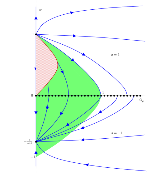
Figure 2: $\Omega_{\rho}-\omega$ plane of the phase space. The shaded region containing flow lines is where $C\geq 0$.

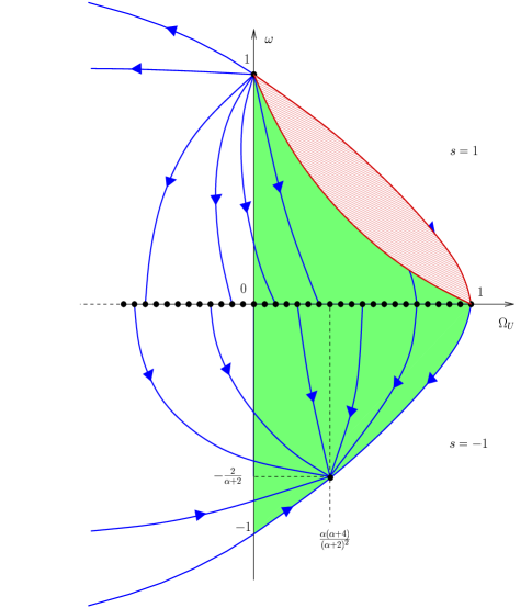
Figure 3: $\Omega_{U}-\omega$ plane of the phase space. The shaded region containing flow lines is where $C\geq 0$.

It is convenient to rewrite the evolution equations with a new time parameter $\tau$, where

$${df\over d\tau}\equiv f^{\prime}=\frac{1}{|\hat{H}|}\frac{df}{d\hat{t}}\,.$$ (31)

Then

$$\hat{H}^{\prime}=-s(1+\hat{q})\hat{H}\,,$$ (32)

where $s={\rm sgn}\,\hat{H}$ and $\hat{q}$ is the deceleration parameter,

$$\hat{q}=-\frac{1}{a^{2}\hat{H}^{2}}\frac{d^{2}{a}}{d\hat{t}^{2}}=1+(\alpha+2)\omega^{2}\,.$$ (33)

The evolution equations for $\Omega$ are then

$$\Omega_{\rho}^{\prime} = s\omega\Omega_{\rho}\left[2(\alpha+2)\omega-\alpha\right]\,,$$ (34)

$$\Omega_{U}^{\prime} = s\omega\left[2(\alpha+2)\omega\Omega_{U}+\alpha(\Omega_{\rho}+2\omega^{2})-2\alpha\omega\right],$$ (35)

$$\omega^{\prime} = s\omega\left[(\alpha+2)\omega^{2}-\alpha\omega-2\right]\,.$$ (36)

Now the Friedmann equation (30) is a constraint on the initial values of $\Omega$. The equilibrium points of the dynamical system $\mbox{\boldmath$\Omega$}^{\prime}=\mbox{\boldmath$f$}(\mbox{\boldmath$\Omega$})$ determined by Eqs. (34)-(36) are solutions of $\mbox{\boldmath$f$}(\mbox{\boldmath$\Omega$}^{\ast})=0$:

$$\mbox{\boldmath$\Omega$}^{\ast}_{1} = (0,0,1)\,,$$ (37)

$$\mbox{\boldmath$\Omega$}^{\ast}_{2} = \left(0,\frac{\alpha(\alpha+4)}{(\alpha+2)^{2}},-\frac{2}{\alpha+2}\right)\,,$$ (38)

$$\mbox{\boldmath$\Omega$}^{\ast}_{3} = (\nu,1-\nu,0)\,.$$ (39)

Actually $\mbox{\boldmath$\Omega$}^{\ast}_{3}$ represents a set of equilibrium points parametrized by $0\leq\nu\leq 1$. The dynamical character of a given equilibrium point $\mbox{\boldmath$\Omega$}^{\ast}$ describes the dynamical behaviour in a small neighbourhood and is determined by the eigenvalues of the matrix Wainwright:1997jw $\mbox{\boldmath$\partial$}_{\mbox{\boldmath$\Omega$}}\mbox{\boldmath$f$}$ at $\mbox{\boldmath$\Omega$}^{\ast}$.

The equilibrium point $\mbox{\boldmath$\Omega$}^{\ast}_{1}$ is a repeller for expanding models. Actually, since $\omega^{\ast}_{1}=1>0$, and considering only models with positive energy density, this point only exists for expanding models ($s=1~{}\Leftrightarrow~{}H>0$). From the fact that this equilibrium point is characterized by $\omega=1$ it follows that $a(t)\propto t^{1/(\alpha+4)}$, and it represents the high energy regime [see Eq. (26)], which is different from the one found in RS2. Moreover, at this equilibrium point we have $\hat{U}=~{}\mbox{constant}$, so there is no flux of gravitons.

The equilibrium point $\mbox{\boldmath$\Omega$}^{\ast}_{2}$ has $\omega^{\ast}_{2}=-2/(\alpha+2)<0$, so that it only exists for contracting models ($s=-1$). At this point, $a(t)\propto(t_{0}-t)^{(\alpha+2)/[2(\alpha+4)]}$ and $C(t)\propto(t_{0}-t)^{-6/(\alpha+4)}$. This equilibrium point, which is an attractor, is the analogous point to $\mbox{\boldmath$\Omega$}^{\ast}_{1}$ for expanding models. Therefore, there is an asymmetry between expanding and contracting models, contrary to what happens in RS2 and general relativistic models Campos:2001pa . This is essentially due to the fact that, unlike in RS2 and general relativity, the dynamical equations on the brane are not invariant under time reversal since there is energy loss to the bulk; specifically, the energy balance equation (12) is not invariant. This asymmetry can be seen in the planes $\Omega_{\rho}-\omega$ and $\Omega_{U}-\omega$ of the phase space shown in Figs. 2 and 3.

The set of points $\mbox{\boldmath$\Omega$}^{\ast}_{3}$ constitutes a line of equilibrium points, which are attractors (repellers) for expanding (contracting) models. At these points, $a(t)\propto t^{1/2}$, the same as in standard radiation models.

The phase space is a non-compact three-dimensional space. For simplicity we only show the projections onto the three possible 2-planes: the $\Omega_{\rho}-\omega$ plane (Fig. 2), the $\Omega_{U}-\omega$ plane (Fig. 3), and the $\Omega_{U}-\Omega_{\rho}$ plane (Fig. 4). These planes describe completely the dynamics of the models. In each of the figures, the (green) shaded region containing flow lines indicates where $C$ is non-negative. In Figs. 2 and 3 the (red) shaded region without flow lines is the region inside the horizon where our equations do not apply. Figures 2 and 3 show the asymmetry between expanding and contracting models, and how the dynamics is determined by the equilibrium points $\mbox{\boldmath$\Omega$}^{\ast}_{1}$ for expanding models (repeller) and $\mbox{\boldmath$\Omega$}^{\ast}_{2}$ for contracting models (attractor).

In Fig. 4 we can see the line of equilibrium points $\mbox{\boldmath$\Omega$}^{\ast}_{3}$ that extends to infinite values of $\Omega_{\rho}$ and $\Omega_{U}$. (Its projection in the other two planes can be seen in Figs. 2 and 3). This plot describes the dynamics for contracting models only, where the point $\mbox{\boldmath$\Omega$}^{\ast}_{2}$ appears. The corresponding one for expanding models can be obtaining by replacing $\mbox{\boldmath$\Omega$}^{\ast}_{2}$ by $\mbox{\boldmath$\Omega$}^{\ast}_{1}$, that is, by moving the equilibrium point to the origin, and inverting the arrows. The three figures show the existence of trajectories on which $\Omega_{U}$, and hence $C$, changes sign, going from negative to positive values. Note that the contrary, to go from positive to negative values of $C$, is forbidden. Expanding models will always end up with a positive $C$.

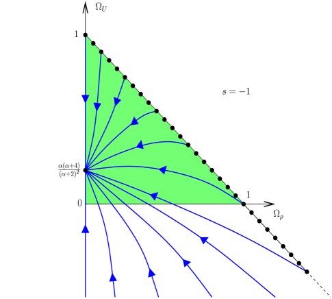
Figure 4: $\Omega_{U}-\Omega_{\rho}$ plane of the phase space. The shaded region is where $C\geq 0$.

V Conclusion

We have investigated the dynamics of a RS2-type braneworld that is radiating 5D gravitons into the bulk during the high-energy radiation (or radiative reheating) era. The simplified model developed in Langlois:2002ke assumes that all gravitons are emitted radially, thus allowing the bulk spacetime to be described by the Vaidya-AdS₅ metric. We found the exact solution in this model to the field equations on the brane, as given in Eqs. (21)–(25). The Weyl radiation term $C/a^{4}$ on the brane, due to the tidal effect of the bulk black hole, is only purely radiative (i.e., $C=\,$const) asymptotically, in the low-energy universe. At early times, $C$ evolves due to graviton emission, with two cases that depend on the choice of an integration constant, as illustrated in Fig. 1. Graviton emission leads to a loss of energy from the brane and a consequent asymmetry between expanding and collapsing models, that is not present in the non-radiating RS2 braneworld. This asymmetry, as well as the asymptotic behaviour of the models at early and late times, is illustrated in the phase planes that fully characterize the dynamics, shown in Figs. 2–4.

Acknowledgements: We thank Arthur Hebecker and Misao Sasaki for useful comments. EL and CFS are supported by EPSRC. RM is supported by PPARC.

References

- (1) K. Ichiki, M. Yahiro, T. Kajino, M. Orito, and G.J. Mathews, Phys. Rev. D66, 043521 (2002) [astro-ph/0203272].
- (2) D. Langlois, L. Sorbo and M. Rodríguez-Martínez, Phys. Rev. Lett. 89, 171301 (2002) [hep-th/0206146].
- (3) A. Hebecker and J. March-Russell, Nucl. Phys. B608, 375 (2001) [hep-ph/0103214]; E. Kiritsis, N. Tetradis, and T. N. Tomaras, JHEP 03, 019 (2002) [arXiv:hep-th/0202037].
- (4) D. Langlois and L. Sorbo, Phys. Rev. D68, 084006 (2003) [hep-th/0306281].
- (5) T. Shiromizu, K. Maeda, and M. Sasaki, Phys. Rev. D62, 024012 (2000) [gr-qc/9910076].
- (6) K. Maeda, S. Mizuno, and T. Torii, Phys. Rev. D 68, 024033 (2003) [gr-qc/0303039].
- (7) A. Chamblin, A. Karch, and A. Nayeri, Phys. Lett. B509, 163 (2001) [hep-th/0007060].
- (8) M. Minamitsuji, M. Sasaki, Phys.Rev. D70 044021 (2004), [gr-qc/0312109].
- (9) A. Campos and C.F. Sopuerta, Phys. Rev. D63, 104012 (2001) [hep-th/0101060]; ibid., D64, 104011 (2001) [hep-th/0105100].
- (10) For details on the use of dynamical systems techniques in cosmology, see: J. Wainwright and G.F.R. Ellis, Dynamical systems in cosmology (Cambridge University Press, 1997).