Generalised Wick Transform in Dimensionally Reduced Gravity

Abstract

In the context of canonical quantum gravity we study an alternative real quantisation scheme, which is arising by relating simpler Riemannian quantum theory to the more complicated physical Lorentzian theory - the generalised Wick transform. On the symmetry reduced models, homogeneous Bianchi cosmology and $2+1$ gravity, we investigate its generalised construction principle, demonstrate that the emerging quantum theory is equivalent to the one obtained from standard quantisation and how to obtain physical states in Lorentzian gravity from Wick transforming solutions of Riemannian quantum theory.

I Introduction

The purpose of this paper is a contribution to the search for quantum gravity, a theory which could describe the quantum behaviour of the full gravitational field Rovelli . This work lies in the canonical line of research which can be characterised by the methodology of attempting to construct a quantum theory in which the Hilbert space carries a representation of the operators corresponding to the metric, without having to fix a background metric. Starting from connection dynamical formulation of general relativity canonical quantisation successfully leads to loop quantum gravity Abhay's Buch . Along these lines, we analyse the utilisation of the generalised Wick transform quantisation method which was first proposed by Thiemann Thiemann's W-paper and then modified by Ashtekar Abhay's W-paper . Its purpose is to simplify the appearance of the last and the key step of the canonical quantisation program, namely solving the scalar constraint $\hat{S}_{L}$.

This strategy to achieve a feasible regularisation for $\hat{S}_{L}$ can be described as follows. We employ the idea to relate mathematically simpler Riemannian quantum theory with the more complicated physical Lorentzian quantum gravity by introducing a generalised Wick transform operator $\hat{\mathbf{W}}$ on the common kinematical Hilbert space of both theories. Classically this strategy arose from a generalised Wick transform where Lorentzian and Riemannian theories are related by a constraint preserving automorphism on the algebra of $\mathbb{C}$ valued functions on the common real phase space of these two theories. This opens up a new avenue within quantum connection dynamics since we will be able to find physical states in real Lorentzian gravity by Wick transforming appropriate solutions of the simpler Riemannian scalar constraint. To complete canonical quantisation, we only have to consider regulating the Wick transform operator $\hat{\mathbf{W}}$ and the simpler Riemannian scalar constraint $\hat{S}_{R}$. In the classical theory the transform is well-defined. In full quantum theory the strategy is attractive but the transform has remained formal. To test if it can be made rigorous and to gain insight into the resulting physical states we will consider simpler symmetry reduced models of $3+1$ gravity, where the issue of regularisation simplifies considerably.

In section III we investigate finite dimensional formulations of spatially homogeneous Bianchi type I and II cosmologies. For these models one already knows what the correct quantisation is. Thus, we will use them to test the viability of the generalised Wick transform strategy and to learn about its technical features. We will observe that the two procedures based respectively on explicit Dirac quantisation of Lorentzian theory and on its indirect quantisation due to the Wick transform program result in identical quantum theories. Furthermore we learn that to obtain physical states from quantum Wick transform, we have to restrict the Hilbert space of Riemannian quantum theory to functions which are subject to additional boundary conditions.

In section IV we turn to the main and most interesting case of $2+1$ gravity. Similarly to our previous Wick transform investigation on Bianchi models, one already knows the resulting quantum theory for Lorentzian $2+1$ gravity. However this quantum theory emerges in a different formulation employing $\mathfrak{su}(1,1)$ variables, rather then in terms of $\mathfrak{su}(2)$ variables as it will be the case from Wick transform quantisation. In order to compare these different quantum theories of $2+1$ gravity and thus to gain insight into the Wick transform technique itself we will first go over to investigate their corresponding classical formulations. In section IV we systematically construct different canonical formulations of $2+1$ dimensional classical general relativity in connection variables and emphasise their practicality for the purpose of canonical quantisation. We will clarify their interplay in sections V and VI by constructing internal phase space maps between them - which we call Wick rotation and Wick transform. They naturally relate Euclidean and Lorentzian formulations of classical $2+1$ gravity. We recover one of them - the Wick transform - as the $2+1$ dimensional analog of our generalised Wick transform in $3+1$ gravity. The other internal phase space map - the Wick rotation - on the classical level also relates $\mathfrak{su}(2)$ Riemannian theory to Lorentzian theory, this time however to its $\mathfrak{su}(1,1)$ appearance.

This new classical perspective of having different classically equivalent formulations of $2+1$ gravity allows considering different implementations of the corresponding quantum Wick transform program. Our main interest is to study the appearance of the Wick transform operator $\hat{\mathbf{W}}$ as defined in Thiemann's W-paper ; Abhay's W-paper , since that represents the general situation which we also encounter for the Wick transform in $3+1$ gravity. In $2+1$ gravity its appearance follows from the particular formulation of classical Lorentzian theory in terms of $\mathfrak{su}(2)$ connections. The direct way to test the corresponding Wick transform quantisation strategy in its $\mathfrak{su}(2)$ formulation will cause, however, regularisation problems and shall be avoided in our further discussion. The simpler framework of $\mathfrak{su}(1,1)$, $2+1$ gravity instead allows to choose an indirect way to test the Wick transform quantisation program. For this purpose, we will construct the Wick rotation - a preliminary technique for our main object of interest the Wick transform in $2+1$ gravity.

In section VI we construct on the classical level a phase space map from Riemannian to Lorentzian theory. In contrast to the generalised Wick transform, where we employ an automorphism on the algebra of phase space functions on the common phase space of both theories, we will now successfully construct a true isomorphism from the phase space of Riemannian theory to the phase space of Lorentzian theory, referred to as internal Wick rotation. Here we approach the main advantage of our alternative construction: (i) one already knows the classical solution space - the cotangent bundle over the moduli space of flat $\mathfrak{su}(2)$, respectively $\mathfrak{su}(1,1)$, connections and (ii) explicit Dirac quantisation of employing operator constraints is equivalent to simpler reduced phase space quantisation. Furthermore, our construction of the internal Wick rotation can be induced to the reduced phase space, thus providing a natural map from ”physical” states of Riemannian quantum theory to physical states of Lorentzian quantum theory. We realise that those internal phase-space maps can not be used to regularise the Wick transform operator $\hat{\mathbf{W}}$ geometrically. However, their importance lies in the possibility to construct the Wick rotation, a Wick transform for $2+1$ gravity, which characterizes the resulting physical states from Wick transform quantisation indirectly. In the case of space-time topology $M^{2,1}\cong T^{2}\times\mathbb{R}$ (where $T^{2}$ is a two-torus) we will study the resulting physical states explicitly. Here we realise that when applied to quantum theory the Wick transform leads us to the most interesting, space-like sector of Lorentzian $2+1$ gravity. Moreover, it turns out that this construction provides a dense subset of the Lorentzian physical Hilbert space.

For a reader who would prefer a self-contained, pedagogical introduction to the subject we recommend Bruno thesis before reading this paper.

II Generalized Wick transform for Gravity

The aim of this section is to briefly review the concept of generalized Wick transform and the quantisation strategy proposed in Thiemann's W-paper ; Abhay's W-paper . Euclidean canonical general relativity expressed in terms of $SU(2)$ connection variables has simple polynomial constraints. Lorentzian theory can be written in terms of the same variables, but the constraints have a complicated form. Thus, the hope is to construct an operator which would allow to map the quantum states of the simpler, Euclidean theory into the Hilbert space of the Lorentzian theory.

First, for motivational purpose, we define an internal phase space isomorphism $\phi$ on the complexified phase space of $\mathfrak{su}(2)$ Riemannian $3+1$ Palatini theory

$$E^{I}_{a} \mapsto iE^{I}_{a}$$

$$K^{I}_{a} \mapsto-iK^{I}_{a}$$

Here, $(E^{a}_{I},K^{I}_{a})$ are the ADM variables (triad and extrinsic curvature) coordinatising the $\mathfrak{su}(2)$ phase-space. Then, we lift $\phi$ to an automorphism on the algebra of $\mathbb{C}$ valued functions on the common real phase space of $\mathfrak{su}(2)$ Riemannian and Lorentzian theory. The result is the following map $\mathbf{W}$, called also the (classical) generalised Wick transform,

$$f\;\;\;\mapsto\;\;\;\mathbf{W}(f)\;=\;f+\{f,T\}+\frac{1}{2!}\{\{f,T\},T\}+\ldots\;=\;\sum^{\infty}_{n=0}\frac{1}{n!}\{f,T\}_{n}$$ (1)

where $T$ is a complex-valued functional given by

$$T:=\frac{i\pi}{2}\int_{\Sigma}d^{3}xK^{I}_{a}E^{a}_{I}$$ (2)

$\mathbf{W}$ is a Poisson bracket-preserving automorphism, it does not commute however with the complex conjugation. The important property of Wick transform from the point of view of the quantisation is that, when applied to Riemannian constraints, it produces the appropriate Lorentzian constraints

$$\begin{array}[]{cccc}\mathbf{W}\>\mathcal{G}_{I}=\mathcal{G}_{I}\;,&\mathbf{W}\>\mathcal{V}_{b}=\mathcal{V}_{b}&\textrm{and}&\mathbf{W}\>\mathcal{S}_{R}=-\>\mathcal{S}_{L}\end{array}$$ (3)

Here, $\mathcal{G}_{I}$, $\mathcal{V}_{b}$ are the Gauss and vector constraints, which have the same form in the two theories. It is only the scalar constraints that are different and therefore we call them $\mathcal{S}_{R}$ and $\mathcal{S}_{L}$ respectively.

Let us now rewrite all constraints in terms of canonically conjugate pair of (connection) variables $(A^{I}_{a},E^{a}_{I})$, which are related to the previous ones via $A^{I}_{a}=\Gamma^{I}_{a}-K^{I}_{a}$ (here $\Gamma$ is the connection compatible with the triad). The Riemannian constraints become at most second order polynomials in basic variables and therefore Riemannian quantum theory is (relatively) easy to solve. Assume we have done that, we can now define the quantum operator corresponding to the Lorentzian scalar constraint using the relation (3). Then, a simple calculation shows that:

$$-\;\hat{\mathcal{S}}_{L}\;:=\;\widehat{\mathbf{W}\mathcal{S}_{R}} = \sum^{\infty}_{n=0}\;\frac{1}{n!}\;{\left(\frac{1}{i\hbar}\right)}^{n}\;[\;\hat{\mathcal{S}_{R}}\;,\>\hat{T}\;]_{n}$$ (4)

$$= exp\;{-\frac{\hat{T}}{i\hbar}}\;\circ\;\hat{\mathcal{S}_{R}}\;\circ\;exp\;{\frac{\hat{T}}{i\hbar}}\;\;=:\;\;\hat{\mathbf{W}}\;\circ\;\hat{\mathcal{S}_{R}}\;\circ\;\hat{\mathbf{W}}^{-1}$$

Here $\hat{T}$ is the operator version of our generating function $T$. In the kinematical Hilbert space $\mathcal{H}_{kin}$ physical quantum states $|\psi\rangle_{L}$, which are defined by $\hat{\mathcal{S}}_{L}|\psi\rangle_{L}:=\hat{\mathbf{W}}\circ\hat{\mathcal{S}_{R}}(\hat{\mathbf{W}}^{-1}|\psi\rangle_{L})=0$, can now be obtained from Wick transforming the kernel of $\hat{\mathcal{S}_{R}}$. Thus the availability of the Wick transform could provide considerable technical simplification: the problem of finding solutions to all quantum constraints is reduced essentially to that of regulating relatively simple operators $\hat{\mathcal{S}}_{R}$ and $\hat{T}$ - in contrast to regularizing the classically more complicated Lorentzian scalar constraint.

For our explicit investigation of the Wick transform quantisation strategy in symmetry reduced models of $3+1$ gravity we will address the kinematical question: Do the constraints $\hat{\mathcal{S}}^{(Wick)}_{L}$ from Wick transform quantisation and $\hat{\mathcal{S}}^{(Dirac)}_{L}$ from standard Dirac quantisation lead to identical quantum theories on $\mathcal{H}_{kin}$? And then the dynamical question: What are the physical states $\hat{\mathbf{W}}|\psi\rangle_{R}\in\mathcal{H}_{phys}$, if $|\psi\rangle_{R}$ is a solution to the Riemannian constraints?

III Bianchi models

In full quantum theory the Wick transform strategy is attractive but the $\hat{\mathbf{W}}$ operator is only defined formally. Our goal is to understand subtleties in making these formal considerations precise. Bianchi models provide a natural arena since in this case one can write out the operators explicitly. In these cases one already knows what the correct answer is. The question is if the Wick transform strategy can be implemented in detail and if it reproduces the correct answer. Thus, the purpose of this section is to use Bianchi models to test the viability of the generalised Wick transform strategy and to learn about its technical features.

In the quantisation strategy of Abhay's W-paper we work exclusively in the real phase space with real constraint functionals. Thus the generalised Wick transform can be used also in equivalent geometrodynamical formulation of $3+1$ gravity. Therein we will study symmetry reduced Bianchi cosmology as a first test model.

To start systematically let us recall the geometrodynamical ADM framework. For space-like foliations $\overset{3,1}{}M\cong\overset{3}{}\Sigma\times\mathbb{R}$ the phase space of our Hamiltonian formulation is coordinatised by the canonical pair $(q_{ab},p^{ab})$ with induced metric $q_{ab}$ to the spatial slice and its conjugate momentum $p^{ab}:=\sqrt{q}(K^{ab}-Kq^{ab})$ which is defined by the extrinsic curvature $K^{ab}$. The Hamiltonian is just a sum of first class constraints. The vector constraint

$$\mathcal{V}_{a}=q_{ab}D_{c}p^{bc}$$ (5)

is independent of the signature. Lorentzian and Riemannian theory differ only in their scalar constraint

$$\mathcal{S}_{L}=+\left(\frac{p^{2}}{2}-p_{ab}p^{ab}\right)+qR \mathcal{S}_{R}=-\left(\frac{p^{2}}{2}-p_{ab}p^{ab}\right)+qR$$ and (6)

The equivalence of the Hamiltonian formulations of $3+1$ Palatini theory and standard Einstein-Hilbert theory allows us to translate the classical Wick transform concept from triads to ADM variables. The induced generator for our generalised Wick transform is now given by

$$T=\frac{i\pi}{2}\int_{\overset{3}{}\Sigma}d^{3}x\;q_{ab}\>p^{ab}$$ (7)

Employing $\mathbf{W}$ as an automorphism on the algebra of phase space functions will again map Riemannian to Lorentzian constraints on the common real phase space of both theories.

In order to simplify the Wick transform quantisation program in terms of ADM variables we will now investigate spatially homogeneous cosmologies as truncated models of $3+1$ gravity. Classically they admit additional symmetries which will simplify the task of quantisation considerably. Spatially homogeneous space-times or Bianchi cosmologies have a $3$-dimensional isometry group $G$ acting simply transitively on a $1$-parameter family of space-like hypersurfaces and hence provide a natural foliation $M\cong G\times\mathbb{R}$ for our Hamiltonian formulation. Therein each hypersurface is isometric to $G$ equipped with a left invariant Riemannian metric. We will further restrict to diagonal, spatially homogeneous models where the $4$-metric expressed in terms of left invariant $1$-forms $\{\omega^{i}_{a}\}_{i=1,2,3}$ can be written as

$$g_{ab}=-N(t)^{2}(dt)_{a}\otimes(dt)_{b}+\sum_{i=1}^{3}q_{i}(t)\omega^{i}_{a}\otimes\omega^{i}_{b}$$ (8)

with purely time dependent lapse function $N(t)$ and diagonal components $q_{i}(t)>0$ of the metric.

We use the ADM framework above to arrive at the Hamiltonian formulation for Bianchi models. For class A Bianchi models homogeneity and diagonal form of the induced metric $q_{ab}$ are compatible with the vacuum field equations since the vector constraint is identically satisfied. Hence we obtain a symmetry reduced ADM formulation which will be the point of departure for canonical quantisation. The reduced configuration space (referred to as minisuperspace) is $3$-dimensional and parameterised by the components of the diagonal spatial metric $q_{i}>0$. The phase space is the cotangent bundle over it with conjugate momenta denoted by $p^{i}$. From the ADM formulation we obtain the induced Poisson bracket relations as $\{q_{i},p^{j}\}=\delta_{i}^{j}$. Only the reduced scalar constraint remains to be imposed in Lorentzian and Riemannian theory

$$\mathcal{S}_{L} =+\left(\frac{{(q_{i}p^{i})}^{2}}{2}-\sum_{i}({q_{i}})^{2}({p^{i}})^{2}\right)+qR$$ (9)

$$\mathcal{S}_{R} =-\left(\frac{{(q_{i}p^{i})}^{2}}{2}-\sum_{i}({q_{i}})^{2}({p^{i}})^{2}\right)+qR$$ (10)

with $q=\det q_{ab}=q_{1}q_{2}q_{3}$ and scalar curvature $R$ of our diagonal spatial metric $q_{ab}$. The symmetry reduced Wick transform generator (7) simplifies to

$$T=\frac{i\pi}{2}q_{i}p^{i}$$ (11)

Misner has introduced a useful parameterisation of the diagonal spatial metric. Incorporating it into a canonical transformation $(q,p)\mapsto(\beta,\pi):=(\ln q,\>qp)$ will further simplify the appearance of our phase space description. In the new canonical variables the non-holonomic constraint $q_{i}>0$ is automatically satisfied - we have trivial phase space topology. Here the scalar constraint of geometrodynamics and our Wick transform generator appear as

$$\mathcal{S}_{L} =+\left(\frac{(\pi_{1}+\pi_{2}+\pi_{3})^{2}}{2}-({\pi_{1}}^{2}+{\pi_{2}}^{2}+{\pi_{3}}^{2})\right)+qR$$ (12)

$$\mathcal{S}_{R} =-\left(\frac{(\pi_{1}+\pi_{2}+\pi_{3})^{2}}{2}-({\pi_{1}}^{2}+{\pi_{2}}^{2}+{\pi_{3}}^{2})\right)+qR$$ (13)

$$T =\frac{i\pi}{2}\;(\pi_{1}+\pi_{2}+\pi_{3})$$ (14)

Let us remark here that, because of this simple form of $T$, in quantum theory there will be no factor ordering problems and one should be able to define a self-adjoint $\hat{\mathbf{W}}$. In the Misner variables the scalar constraint has the familiar form of a sum of a kinetic term and a potential term $qR$, which depends on the specific Bianchi model under consideration. We will use our Misner parameterisation as the point of departure for canonical quantisation of Bianchi I and Bianchi II cosmology in the next sections.

III.1 Wick transform for Bianchi I

We now want to exploit the simplicity of the scalar constraint (12, 13) in Bianchi I cosmology. As mentioned before, Bianchi models are characterised by their Lie algebras. For Bianchi I the structure constants vanish completely. Thus the spatial, homogeneous, diagonal metric is flat and the potential term in the scalar constraint disappears entirely. We find identical classical phase space description for Riemannian and Lorentzian theory, since $\mathcal{S}_{R}=-\mathcal{S}_{L}$.

To evaluate our quantum Wick transform program we have to quantise Bianchi I cosmology by employing the Dirac procedure of imposing operator constraints to select the physical states. This can be achieved by performing the following steps

(i) quantise the kinematical phase space, i.e. represent the Poisson algebra of kinematical phase space functions by an algebra of operators on the kinematical Hilbert space $\mathcal{H}_{kin}$.

(ii) restrict to the physical Hilbert space $\mathcal{H}_{phys}\subset\mathcal{H}_{kin}$ which is defined as the solution space to the quantum constraints. All quantised Dirac observables leave that subspace invariant and can therefore be reduced to $\mathcal{H}_{phys}$.

(iii) select a scalar product on the space of physical states by demanding that quantised physical observables be promoted to self adjoint operators on $\mathcal{H}_{phys}$. This can be indirectly achieved by representing all Dirac observables (what includes the set of physical observables) - i.e. all operators which leave $\mathcal{H}_{phys}$ invariant - by self adjoint operators. Here it is sufficient to impose that reality condition on a complete set of generators on the algebra of Dirac observables.

The simplicity of Bianchi I theory allows us to find an explicit solution space to the quantum constraints as well as a complete set of Dirac observables and thus to carry out the quantisation program to completion. We start to quantise our constraint system in the Misner phase space parameterisation (12, 13) and implement the program step by step.

We first quantise the kinematical phase space which is topologically $\mathbb{R}^{6}$ and parameterised by the canonical pair $(\beta_{i},\pi_{i})$. In the passage to quantum theory lets consider $\mathcal{H}_{kin}=L^{2}(\mathbb{R}^{3})$ to arise from the space of distributions $\psi$ over the configuration space. Thereon we represent our Poisson algebra of canonical pairs $(\beta_{i},\pi_{i})$ by an algebra of configuration operators $\hat{\beta_{i}}:=\beta_{i}\cdot\>$ and momentum operators $\hat{\pi_{i}}:=-i\hbar\partial/\partial\beta_{i}$.

The next task is to single out the physical Hilbert space $\mathcal{H}_{phys}$ by solving the quantum constraint

$$-\hat{\mathcal{S}}_{L}=\hat{\mathcal{S}}_{R}=\hbar^{2}\left[\frac{1}{2}\left(\frac{\partial}{\partial\beta_{1}}+\frac{\partial}{\partial\beta_{2}}+\frac{\partial}{\partial\beta_{3}}\right)^{2}-\left(\frac{\partial^{2}}{{\partial\beta_{1}}^{2}}+\frac{\partial^{2}}{{\partial\beta_{2}}^{2}}+\frac{\partial^{2}}{{\partial\beta_{3}}^{2}}\right)\right]$$ (15)

We can diagonalise $\hat{\mathcal{S}}_{R}$ by employing a linear coordinate transformation on the configuration space

$$\left(\begin{array}[]{c}\beta_{0}\\ \beta_{+}\\ \beta_{-}\end{array}\right):=\frac{1}{3}\left(\begin{array}[]{ccc}1&1&1\\ -1&-1&2\\ -1&2&-1\end{array}\right)\left(\begin{array}[]{c}\beta_{1}\\ \beta_{2}\\ \beta_{3}\end{array}\right)$$ (16)

Finally we obtain our quantised scalar constraint (15) and Wick transform generator (14) as

$$\hat{\mathcal{S}}_{R} =-\hat{\mathcal{S}}_{L}=\>-\>\frac{3}{2}\>\hbar^{2}\left(-\frac{\partial^{2}}{{\partial\beta_{0}}^{2}}+\frac{\partial^{2}}{{\partial\beta_{+}}^{2}}+\frac{\partial^{2}}{{\partial\beta_{-}}^{2}}\right)=-\>\frac{3}{2}\>\hbar^{2}\;\Box$$ (17)

$$\hat{T} =\>\frac{3}{2}\>\pi\hbar\;\frac{\partial}{\partial\beta_{0}}$$ (18)

Thus our space of physical states $\mathcal{H}_{phys}$ will arise from solutions to the quantum constraint equation $\Box\>\psi=0$. Or, after employing a Fourier transform, in the unitarily equivalent momentum representation from solutions of $(-{\pi_{0}}^{2}+{\pi_{+}}^{2}+{\pi_{-}}^{2})\>\varphi=0$, which are spanned by states of the form:

$$\varphi_{phys}(\pi):=\delta(\pi_{0}-\sqrt{{\pi_{+}}^{2}+{\pi_{-}}^{2}})\cdot\varphi(\widetilde{\pi})$$ (19)

where $\varphi_{phys}$ is a distribution on the kinematical configuration space $\mathbb{R}^{3}$ and $\varphi\in L^{2}(\mathcal{L})$ a square integrable function on the light cone $\mathcal{L}\subset\mathbb{R}^{3}$. From the simple scalar constraint, a function of $\pi_{i}$ alone, we obtain a common pre-factor $\delta(\pi_{0}-\sqrt{{\pi_{+}}^{2}+{\pi_{-}}^{2}})$ to all distributional solutions. Hence each state $\varphi_{phys}$ is completely characterised by functions $\varphi\in L^{2}(\mathcal{L})$ on the light-cone, which shall be used from now on to represent elements in $\mathcal{H}_{phys}$.

The next step in our quantisation procedure is to find a complete set of Dirac observables. In momentum representation a complete set of differential operators on $L^{2}(\mathbb{R}^{3})$ which leaves $L^{2}(\mathcal{L})$ invariant can contain arbitrary configuration operators - here we select operator analogs to the functions $(\pi_{+},\pi_{-})$. However the vector fields corresponding to the momentum operators therein are restricted to lie in the tangent space $T\mathcal{L}$. We find a complete set of them from the canonical immersion

$$\begin{array}[]{cccc}\phi:&\mathbb{R}^{2}&\rightarrow&\mathcal{L}\;\;\;\;\subset\;\;\;\;\mathbb{R}^{3}\\ &(\tilde{\pi}_{+},\tilde{\pi}_{-})&\mapsto&(\sqrt{{\tilde{\pi}_{+}}^{2}+{\tilde{\pi}_{-}}^{2}},\tilde{\pi}_{+},\tilde{\pi}_{-})\end{array}$$ (20)

of the light cone into the kinematical configuration space. Here we choose momentum operators which are slightly different from the canonical base vector fields

$$\hat{v}_{+} := \pi_{0}\cdot d\phi\left(\frac{\partial}{\partial\tilde{\pi}_{+}}\right)=\pi_{0}\frac{\partial}{\partial\pi_{+}}+\pi_{+}\frac{\partial}{\partial\pi_{0}}$$ (21)

$$\hat{v}_{-} := \pi_{0}\cdot d\phi\left(\frac{\partial}{\partial\tilde{\pi}_{-}}\right)=\pi_{0}\frac{\partial}{\partial\pi_{-}}+\pi_{-}\frac{\partial}{\partial\pi_{0}}$$ (22)

The set of operators $(\hat{\pi}_{+},\hat{\pi}_{-},\hat{v}_{+},\hat{v}_{-})$ obviously generates the entire algebra of Dirac observables on $\mathcal{H}_{phys}$ (in momentum representation). A straightforward computation of their Lie brackets shows, that the above set of generators enlarged by the two algebraically related operators $\hat{v}_{0}:=[\hat{v}_{+},\hat{v}_{-}]=-\pi_{-}\frac{\partial}{\partial\pi_{+}}+\pi_{+}\frac{\partial}{\partial\pi_{-}}$ and $\hat{\pi}_{0}=[\hat{v}_{\pm},\hat{\pi}_{\pm}]$ forms a Lie algebra which is isomorphic to the Lie algebra of the Poincare group in 3-dimensional Minkowski space.

We complete our quantisation procedure by specifying an inner product on $\mathcal{H}_{phys}=L^{2}(\mathcal{L},\mu)$ in a way that Dirac operators corresponding to real physical observables are self adjoint. Here it is sufficient to impose that reality condition to our complete set of generators on the algebra of Dirac observables. For any two physical states $\varphi,\psi\in\mathcal{H}_{phys}$ our inner product

$$\langle\varphi,\psi\rangle=\int_{\mathcal{L}}\bar{\varphi}\>\psi\;\mu$$ (23)

is determined by the measure $\mu$ on the light cone $\mathcal{L}$. Regarding our choice of momentum operators $\hat{v}_{I}$ we find the most convenient measure on $L^{2}(\mathcal{L},\mu)$ by employing our immersion $(\ref{Licht-Kegel-Immersion})$ to the standard flat measure on $\mathbb{R}^{3}$ to get $\phi^{\ast}\mu_{0}=\frac{1}{\pi_{0}}\>d\tilde{\pi}_{+}\wedge d\tilde{\pi}_{-}$ with respect to which the pulled back vector fields $v_{I}$ are divergence-free. Finally we approach our desired goal and prove their corresponding momentum operators $\hat{v}_{I}$ to be self adjoint on $L^{2}(\mathcal{L},\;\mu_{0}|_{\mathcal{L}}\>:=\frac{1}{\pi_{0}}\>d\pi_{+}\wedge d\pi_{-})$.

This completes the implementation of Dirac’s quantisation program for the Riemannian and Lorentzian Bianchi type I model. In the final picture we describe the Hilbert space of physical states in its momentum representation by $L^{2}(\mathcal{L},\;\mu_{0})$. Thereon we find the Wick transform generator (18) in the simplified form

$$\hat{T}=\>-\>i\>\frac{3}{2}\>\pi\hbar\;\pi_{0}$$ (24)

Thus $\hat{T}$ is anti self-adjoint, whence $\mathbf{\hat{W}}$ is self-adjoint.

Now we have everything together to test our quantum Wick transform concept in the symmetry reduced Bianchi I model. We will explicitly compare the two quantum theories based respectively on Wick transform quantisation and on the previously introduced Dirac procedure. In the degenerate case of Bianchi type I we will find both schemes to be equivalent.

The idea was to solve the scalar constraint for Lorentzian gravity by Wick transforming solutions of the scalar constraint of Riemannian theory. The first issue to discuss was the regularisation of the corresponding Wick transform operator $\hat{\mathbf{W}}$. Due to the simple appearance of its generator $\hat{T}$ the Wick transform operator is obviously well defined

$$\hat{\mathbf{W}}=\exp\left(-\frac{1}{i\hbar}\hat{T}\right)=\exp\left(\frac{3}{2}\>\pi\>\hat{\pi}_{0}\right)$$ (25)

On the kinematical Hilbert space (in momentum representation) we further realise that both Lorentzian scalar constraint operators which arise from Wick transform quantisation or from Dirac’s procedure in (17) are identical

$$\hat{\mathcal{S}}_{L}^{(\textrm{Wick})}:=-\hat{\mathbf{W}}\;\circ\;\hat{\mathcal{S}_{R}}\;\circ\;\hat{\mathbf{W}}^{-1}$$ (26)

$$=-\exp\left(\frac{3}{2}\pi\hat{\pi}_{0}\right)\cdot\frac{(-3)}{2}\hbar^{2}(-{\pi_{0}}^{2}+{\pi_{+}}^{2}+{\pi_{-}}^{2})\exp\left(-\frac{3}{2}\pi\hat{\pi}_{0}\right)=\hat{\mathcal{S}}_{L}^{(\textrm{Dirac})}$$ (27)

where the Riemannian scalar constraint (17) is also chosen in momentum representation.

The final step in our Wick transform quantisation program is to introduce an inner product on the space of physical states $\mathcal{H}_{phys}$. Following our strategy to obtain (normalised) physical states $|\varphi_{L}\rangle:=\hat{\mathbf{W}}|\varphi_{R}\rangle$ in Lorentzian theory from Wick transforming solutions of the Riemannian scalar constraint, we seek for a criterion how to select appropriate $|\varphi_{R}\rangle$ in the solution space $\textrm{Ker}(\hat{\mathcal{S}}_{R})$ of the Riemannian scalar constraint (with $\>\textrm{Ker}(\hat{\mathcal{S}}_{R})$ described by the space of arbitrary functions on the light cone $\mathcal{L}$). For Bianchi I we already know $\mathcal{H}_{phys}$ from our previous Dirac quantisation method. Thus we easily find the desired set of appropriate Riemannian solutions $|\varphi_{R}\rangle\in\textrm{Ker}(\hat{\mathcal{S}}_{R})$ from utilising the inverse Wick transform operator as $\hat{\mathbf{W}}^{-1}\circ\mathcal{H}_{phys}\subset\textrm{Ker}(\hat{\mathcal{S}}_{R})$. Finally we can characterise the subspace $\hat{\mathbf{W}}^{-1}\circ\mathcal{H}_{phys}$ of appropriate solutions to the Riemannian scalar constraint as the space of all functions

$$\varphi_{R}:=\varphi\cdot\exp\left(-\frac{3}{2}\pi\pi_{0}\right) \varphi\in L^{2}(\mathcal{L},\mu_{0}|_{\mathcal{L}}=\frac{1}{\pi_{0}}\>d\pi_{+}\wedge d\pi_{-})$$ with (28)

We learn that to obtain (normalised) physical states from quantum Wick transform we have to restrict to the above subspace in the Hilbert space $L^{2}(\mathcal{L},\mu_{0}|_{\mathcal{L}})$ of Riemannian quantum theory. In contrast general solutions in Riemannian quantum theory might get Wick transformed to functions which diverge at the boundary of the configuration space.

III.2 Wick transform for Bianchi II

In order to canonically quantise class A Bianchi models we chose to start classically from their parameterisation in terms of Misner variables. Only the Riemannian or Lorentzian scalar constraint (13, 12) remains to be solved, where the potential term $qR$ depends on the type of Bianchi model. The explicit common quantisation of both Riemannian and Lorentzian Bianchi type I models was easy to accomplish because they are flat. Now we want to study the simplest representative for the remaining Bianchi models with non-vanishing potential term: that is Bianchi type II.

Let us recall that Bianchi cosmologies are classified by the Lie algebra which corresponds to their isometry group. In class A Bianchi models structure constants are trace free and can therefore be expressed in terms of a symmetric matrix $n^{ab}$: ${C^{a}}_{bc}=\epsilon_{mbc}n^{ma}$, where $\epsilon_{mbc}$ is the total antisymmetric symbol. In the type II model $n^{ab}$ has signature $(0,0,+)$. Without loss of generality we can assume diagonal form $n^{ab}=\textrm{diag}(0,0,n)^{ab}$. Employing the simple structure of the Lie algebra and starting from the diagonal form (8) of our spatial homogeneous metric $q_{ab}$ the scalar curvature $R$ is obtained from a straightforward computation as

$$R=-n^{2}\frac{q_{3}}{q_{1}q_{2}}$$ (29)

Hence we find for Bianchi type II the scalar constraints (12, 13) equipped with the simple potential term $qR=-\>n^{2}\cdot{q_{3}}^{2}$. Expressed in the canonically conjugate Misner variables $(\beta_{i},\pi_{i})$ we obtain Lorentzian and Riemannian scalar constraint as well as the Wick transform generator $T$ as

$$\mathcal{S}_{L} =+\left(\frac{(\pi_{1}+\pi_{2}+\pi_{3})^{2}}{2}-({\pi_{1}}^{2}+{\pi_{2}}^{2}+{\pi_{3}}^{2})\right)-\>n^{2}e^{2\beta_{3}}$$ (30)

$$\mathcal{S}_{R} =-\left(\frac{(\pi_{1}+\pi_{2}+\pi_{3})^{2}}{2}-({\pi_{1}}^{2}+{\pi_{2}}^{2}+{\pi_{3}}^{2})\right)-\>n^{2}e^{2\beta_{3}}$$ (31)

$$T =\frac{i\pi}{2}\;(\pi_{1}+\pi_{2}+\pi_{3})$$ (32)

As in our quantum Wick transform investigation in the degenerate Bianchi type I model in section III.1, we will use this Hamiltonian phase space description as the starting point for quantisation á la Dirac.

First we quantise the kinematical phase space and obtain the same kinematical Hilbert space $\mathcal{H}_{kin}=L^{2}(\mathbb{R}^{3})$ as before constrained by operators analogous to $\hat{\mathcal{S}}_{R}$ and $\hat{\mathcal{S}}_{L}$ in (15) which are supplemented with the potential term $-n^{2}e^{2\beta_{3}}$. To simplify the appearance of these operators we employ the same coordinate transformation on the configuration space and obtain the quantised scalar constraints and Wick transform generator as

$$\hat{\mathcal{S}}_{L} =\>+\>\frac{3}{2}\>\hbar^{2}\;\Box\;-\;n^{2}\>e^{2\beta_{0}}\>e^{2\beta_{+}}$$ (33)

$$\hat{\mathcal{S}}_{R} =\>-\>\frac{3}{2}\>\hbar^{2}\;\Box\;-\;n^{2}\>e^{2\beta_{0}}\>e^{2\beta_{+}}$$ (34)

$$\hat{T} =\>\frac{3}{2}\>\pi\hbar\>\frac{\partial}{\partial\beta_{0}}$$ (35)

In contrast to Bianchi type I quantisation the solution space to the more complicated Riemannian and Lorentzian constraint operator is not obvious at all. Since we have no explicit expression for the physical Hilbert space $\mathcal{H}_{phys}$ we will not complete Dirac’s quantisation procedure and therefore not Wick transform physical states. We finish our investigation of Bianchi type II by studying the quantum Wick transform kinematically. Similar to its implementation on Bianchi type I, we find on $\mathcal{H}_{kin}$ that the two formulations based respectively on Wick transform quantisation and explicit Dirac quantisation are equivalent.

First we study the regularisation of the corresponding Wick transform operator. Like in our previous Bianchi I quantisation (25) we obtain

$$\hat{\mathbf{W}}=\exp\left(-\frac{1}{i\hbar}\hat{T}\right)=\exp\left(i\>\frac{3}{2}\>\pi\>\frac{\partial}{\partial\beta_{0}}\right)$$ (36)

as the exponential of an anti self-adjoint operator, i.e. $\hat{\mathbf{W}}$ is well defined. On the kinematical Hilbert space we further realise that both Lorentzian constraints $\hat{\mathcal{S}}_{L}^{\textrm{(Dirac)}}$ and $\hat{\mathcal{S}}_{L}^{\textrm{(Wick)}}$ which arise from Dirac’s procedure in (33) and, respectively, from Wick transform quantisation are identical

$$\hat{\mathcal{S}}_{L}^{(\textrm{Wick})}:= -\hat{\mathbf{W}}\;\circ\;\hat{\mathcal{S}_{R}}\;\circ\;\hat{\mathbf{W}}^{-1}$$ (37)

$$= -\exp\left(i\frac{3}{2}\pi\frac{\partial}{\partial\beta_{0}}\right)\circ\left(-\frac{3}{2}\hbar^{2}\Box-n^{2}e^{2\beta_{0}}e^{2\beta_{+}}\right)\circ\exp\left(-i\frac{3}{2}\pi\frac{\partial}{\partial\beta_{0}}\right)$$ (38)

$$= -\left(-\frac{3}{2}\hbar^{2}\>\Box\;+\;n^{2}e^{2\beta_{0}}e^{2\beta_{+}}\right)=\hat{\mathcal{S}}_{L}^{(\textrm{Dirac})}$$ (39)

To summarise our investigation of the quantum Wick transform program on Bianchi type I and II we can conclude that restricted to these test models there is no regularisation problem for $\hat{\mathbf{W}}$ arising, what one might expect due to its complicated definition. Employing canonical transformations to these symmetry reduced ADM formulations simplified the generalised Wick transform operator considerably. We observe that the classically equivalent appearance of the Lorentzian scalar constraint arising from generalised Wick transform results after canonical quantisation in the same constraint operator $\hat{\mathcal{S}}_{L}^{(\textrm{Wick})}$ as the one obtained from direct canonical quantisation of the Lorentzian scalar constraint $\hat{\mathcal{S}}_{L}^{(\textrm{Dirac})}$. Our test on Bianchi models shows, that the generalised Wick transform can be implemented in detail and reproduced the same quantum theory as explicit Dirac quantisation. Furthermore we explicitly observed in our Bianchi type I quantisation, that to obtain physical states from quantum Wick transform, we have to restrict the Hilbert space of Riemannian quantum theory to functions which are subject to additional boundary conditions.

IV $2+1$ Palatini theory

In this section we turn to the main and most interesting case of $2+1$ gravity. Similarly to our investigation on Bianchi models our goal is to use the symmetry reduced framework of $2+1$ gravity to study the Wick transform quantisation programme by comparing the emerging quantum theory with known results from standard quantisation.

In this section, we will be mainly concerned with classical $2+1$ Palatini theory and discuss canonical quantisation later on. Here we describe different formulations of $2+1$ dimensional classical general relativity in vacuum. In our Hamiltonian description the pair of canonically conjugate variables is given by a connection one-form $A^{I}_{a}$ and a densitized dyad $E^{I}_{a}$. Our descriptions will differ depending on their gauge group choice in the vector bundle formulation. According to the variables chosen our theories will represent either Riemannian or Lorentzian gravity. Furthermore we describe two Lorentzian theories and obtain different sets of associated constraints which are very similar to constraints encountered in $3+1$ gravity between the $SU(2)$ and $SL(2,\mathbb{C})$ Lorentzian theories. Later, by relating these classical Lorentzian theories to Riemannian theory, we will construct and study different implementations of the corresponding quantum Wick transform program.

IV.1 $\mathfrak{su}(2)$ Riemannian   and   $\mathfrak{su}(1,1)$ Lorentzian $2+1$ theory

Let us briefly introduce the Hamiltonian formulation of $2+1$ Palatini theory following the detailed implementation and notation in the review article by Romano Romano . The classical Lagrangian starting point is standard Einstein-Hilbert action in metric variables. We introduce triads as soldering forms which provide an isomorphism $e^{I}_{a}(p):T_{p}M\rightarrow\mathfrak{g}$. For Riemannian theory we choose $\mathfrak{g}$ to be $\mathfrak{su}(2)$ and for Lorentzian gravity $\mathfrak{su}(1,1)$. Then, we find an equivalent configuration space description by reformulating the Einstein-Hilbert action as a functional of triads $e^{I}_{a}$ and connections $A^{I}_{a}$. We obtain the $2+1$ Palatini action as

$$S_{P}(A,e):=\frac{1}{4}\int_{M}\tilde{\eta}^{abc}e_{aI}F^{I}_{bc}$$ (40)

where $\tilde{\eta}^{abc}$ represents the densitized volume form and $F^{I}_{ab}=2\partial_{[a}A^{I}_{b]}+[A_{a},A_{b}]^{I}$ is the curvature of the covariant derivative $D_{a}=\partial_{a}+[A_{a},\cdot]$ which is determined by the connection $A^{I}_{a}$. When we vary $S_{P}(A,e)$ with respect to connections and triads we obtain two Euler-Lagrange equations of motion which are again equivalent to standard Einstein equation in metric variables.

To provide the point of departure for canonical quantisation we will now move over to the Hamiltonian formulation. Let our base manifold $M\cong\Sigma\times\mathbb{R}$ be foliated by the images of a one-parameter family of embeddings $\mathcal{E}_{t}:\Sigma\rightarrow\Sigma_{t}\subset M$. For simplicity we further assume $\Sigma$ to be compact. Here $\mathbb{R}$ coordinates represent evolution parameter from one $2$-dimensional $t=const.$ surface $\Sigma_{t}$ to the other, which does not necessarily have the interpretation of time. This is where a conceptual difference to $3+1$ Palatini theory arises, where we allowed space-like foliations only. Now we use arbitrary foliations! After performing the Legendre transform we obtain the resulting Hamilton description as follows. The phase space consists of pairs $(A^{I}_{a},E^{J}_{b})$, where $A^{I}_{a}$ is the pull back of the connection to the $2$-dimensional slice $\Sigma$ and $E^{J}_{b}$, its conjugate momentum, is the pull back of our triads to $\Sigma$ with density weight one. For convenience we will call $E^{I}_{a}$ dyad from now on. Following Dirac constraint analysis we find, similarly as in $3+1$ Palatini theory, our Hamiltonian as a linear combination of Gauss and curvature constraint functions

$$\mathcal{G}_{I} := D_{a}E^{a}_{I}=0$$ (41)

$$\mathcal{F}_{ab}^{I} := F^{I}_{ab}=0$$ (42)

which are independent of the signature and remarkably only linear or independent in momenta $E^{I}_{a}$. In contrast to $3+1$ gravity, where we encountered additional second class constraints, in $2+1$ Palatini theory the constraint system is first class. Given a test field $v^{I}$ the Gauss constraint Hamiltonian vector field generates infinitesimal vector bundle gauge transformations

$$A^{I}_{a} \mapsto A^{I}_{a}-\epsilon D_{a}v^{I}$$ (43)

$$E^{I}_{a} \mapsto E^{I}_{a}-\epsilon[v,E_{a}]^{I}$$ (44)

which similarly arise in Yang-Mills theory. The $1$-parameter family of diffeomorphisms generated by the curvature constraint Hamiltonian vector field is

$$A^{I}_{a} \mapsto A^{I}_{a}$$ (45)

$$E^{I}_{a} \mapsto E^{I}_{a}+\epsilon D_{a}v^{I}$$ (46)

To summarise, our constrained Hamiltonian system is parameterised by $\mathfrak{g}$-valued connections $A^{I}_{a}$ and dyads $E^{I}_{a}$ which obey first class constraints (41) and (42). In our Palatini formulation Riemannian and Lorentzian $2+1$ gravity are only distinguished by their internal vector space $\mathfrak{su}(2)$ and $\mathfrak{su}(1,1)$, respectively.

For non-degenerate dyads $\mathcal{F}$ can be decomposed into its ”normal” and ”tangential” internal vector space component to obtain Gauss, vector and scalar constraint which are similar to constraints encountered in $3+1$ gravity

$$\mathcal{G}_{I} =D_{a}E^{a}_{I}=0$$ (47)

$$\mathcal{V}_{b} =E^{a}_{I}F^{I}_{ab}=0$$ (48)

$$\mathcal{S} =\varepsilon_{IJK}E^{Ia}E^{Jb}F^{K}_{ab}=0$$ (49)

IV.2 Lorentzian $2+1$ theory using $\mathfrak{su}(2)$

So far our Lorentzian theory uses $\mathfrak{su}(1,1)$ valued dyads and connections as phase space variables. We will now provide an alternative formulation of Lorentzian $2+1$ gravity using $\mathfrak{su}(2)$ valued dyads and connections, i.e. embedded into the same phase space as Riemannian theory. To achieve that formulation we will first understand how our present Lorentzian $\mathfrak{su}(1,1)$ theory naturally arises by symmetry reduction of full Lorentzian $3+1$ gravity. Using an alternative reduction process we will finally obtain Lorentzian $2+1$ Palatini theory in terms of $\mathfrak{su}(2)$ variables.

Let us now rediscover Lorentzian $2+1$ Palatini theory as a suitable Killing reduction of Lorentzian $3+1$ Palatini theory. In that case we will assume the existence of a fixed spatial symmetry represented by a constant Killing vector field $\xi^{a}$, such that our base manifold foliates $\overset{3,1}{}M\cong\overset{2,1}{}\Sigma\times\mathbb{R}$ with $\mathbb{R}$ representing space-like integral curves of $\xi^{a}$. We decompose the Lorentzian $3+1$ Palatini action with respect to the given symmetry induced foliation. The result is analogous to the well known space-time decomposition of the $3+1$ Palatini action. In order to reduce this action to the previously discussed Lorentzian $2+1$ Palatini action (40) with gauge group $SO(2,1)$ we have to impose the following obvious conditions: (i) gauge fix our tetrads to $(\overset{4}{}e\cdot\xi)^{i}=const.$ and (ii) gauge fix our connections by $\mathcal{L}_{\vec{\xi}}\;\overset{4}{}A_{a}^{ij}=0$ and $(\xi\cdot\overset{4}{}A)^{ij}=0$. Effectively we partially gauge fix our tetrads and connections onto the section $\overset{2,1}{}\Sigma$ which arose from the foliation pursuant to the fixed spatial symmetry.

Partially gauge fixed action can be immediately identified with Lorentzian $2+1$ Palatini action (40) where we use $\mathfrak{su}(1,1)$ phase space variables. According to our previous discussion we move over to its Hamiltonian description using arbitrary foliations on $\overset{2,1}{}\Sigma$ consequently without further gauge fixing. Eventually we find a Killing reduced version of Lorentzian $3+1$ Palatini theory which is identical to $\mathfrak{su}(1,1)$ Lorentzian $2+1$ Palatini theory.

In the following symmetry based reduction process of Lorentzian $3+1$ Palatini theory we again assume the existence of a fixed spatial symmetry represented by a constant space-like Killing vector field $\xi^{a}$. In particular this indirectly gauge fixes our tetrads to be adapted to the foliation induced by $\xi^{a}$ and constant along $\xi^{a}$. But in contrast to the previous reduction, where we first decomposed our gauge restricted Palatini action with respect to the symmetry and afterwards with respect to an arbitrary space-time foliation, we will now start with a suitable space-time decomposition. Consequently we first enter the Hamiltonian formulation of $3+1$ Palatini theory where we restrict ourselves to space-like foliations $\overset{3,1}{}M\cong\overset{3}{}\Sigma\times\mathbb{R}$ whereas our symmetry further restricts our triads to be constant along $\xi^{a}$ in the spatial slice $\overset{3}{}\Sigma$. That additional limitation has no influence to the Dirac constraint analysis. Therefore the reduced phase space of Lorentzian $3+1$ Palatini theory is parameterised by the $\mathfrak{so}(3)$ valued pair $(E^{a}_{I},K^{I}_{a})$ on $\overset{3}{}\Sigma$ and subject to Gauss, vector and scalar constraint

$$\mathcal{G}_{I} :=\varepsilon_{IJK}K^{J}_{a}E^{aK}=0$$

$$\mathcal{V}_{b} :=2E^{a}_{I}D_{[a}K^{I}_{b]}=0$$

$$\mathcal{S}_{L} :=-qR+2E^{[a}_{I}E^{b]}_{J}K^{J}_{a}K^{I}_{b}=0$$

Again the remnant of our additional spatial symmetry in $\overset{3}{}\Sigma$ restricts our non-degenerate triads $E^{a}_{I}$ to be constant along $\xi^{a}$. Thus our reduced phase space variables $(E^{a}_{I},K^{I}_{a})$ can be properly induced to another foliation $\overset{3}{}\Sigma\cong\overset{2}{}\Sigma\times\mathbb{R}$ with respect to the symmetry. They are represented by their pull backs to $\overset{2}{}\Sigma$ and subject to the induced constraints. We can pass back to connection dynamics by employing canonical transformation $(E^{a}_{I},K_{a}^{I})\mapsto(A^{I}_{a},E^{a}_{I})$ and obtain the associated connection dynamical description in terms of $\mathfrak{su}(2)$-valued pairs $(A^{I}_{a},E^{a}_{I})$ with induced Gauss, vector and scalar constraints

$$\mathcal{G}_{I} :=D_{a}E^{a}_{I}=0$$ (50)

$$\mathcal{V}_{b} :=E^{a}_{I}F^{I}_{ab}=0$$ (51)

$$\mathcal{S}_{L} :=\varepsilon_{IJK}E^{Ia}E^{Jb}F^{K}_{ab}+4E^{[a}_{I}E^{b]}_{J}K^{J}_{a}K^{I}_{b}=0$$ (52)

The slightly more complicated structure of $\mathcal{S}_{L}$ is the same which we encounter in $3+1$ Palatini theory during explicit canonical transformation of the scalar constraint in ADM-variables to the scalar constraint in connection variables.

Thus, performing an alternative symmetry reduction for Lorentzian $3+1$ Palatini theory we have obtained an equivalent formulation for Lorentzian $2+1$ Palatini theory in terms of $\mathfrak{su}(2)$ valued connections and dyads $(A,E)$. The constraints for those variables are more complicated than in the $\mathfrak{su}(1,1)$ formulation. This is the price we pay for having a compact gauge group rather than a non-compact one. Effectively we describe Lorentzian $2+1$ theory on the same phase space as Riemannian theory subject to the same constraints with the only exception that the scalar constraint (49) is replaced by (52). In order to further clarify the relations between various variables discussed above we provide a schematic description in the figure 1. Notice also that the formulation of the Lorentzian theory with a compact gauge group allows us to perform rigorous constructions of various quantum operators within canonical quantisation programme. Such constructions for the area and the Hamiltonian operators are given in thesis . The constructions are analogous to the ones already known from the $3+1$ theory.

Figure 1: Relations between different variables

IV.3 Natural maps between these theories

So far we have various connection dynamical formulations of $2+1$ dimensional classical general relativity. They differ (i) by their gauge group choice in the vector bundle formulation, (ii) represent either Riemannian or Lorentzian gravity, (iii) their scalar constraint $\mathcal{S}$ is either simply polynomial or difficult and (iv) they can use real or complex connections. From the viewpoint of canonical quantum gravity, the quantisation strategy is easier if we have compact gauge group, polynomial constraints and work entirely with real connections. To represent a physical theory we have to quantise Lorentzian gravity. We realise that in all our formulations for $2+1$ dimensional gravity introduced in the last two subsections we have abandoned one of these simple structures. The situation is illustrated in figure 2.

Figure 2: Overview of the situation

The situation is analogous to full $3+1$ gravity. Using an observation due to Thiemann Thiemann's W-paper , a generalised Wick transform allows us to circumvent that drawback and opens up a new avenue within quantum connection dynamics. The Wick transform strategy was to utilise a sufficiently simple, constraint preserving, phase space map from the mathematically simpler Riemannian theory to a more complicated physical Lorentzian theory, which shall be used in quantisation to relate the corresponding quantum theories. We will call that type of phase space maps internal, because they leave our real space-time base manifold unchanged, are restricted to the fibre in our vector bundle formulation and substitute the signature therein.

V $2+1$ Wick transform

Let us now investigate the quantum Wick transform in $2+1$ Palatini theory. There are two classically equivalent formulations of Lorentzian theory which naturally relate to Riemannian theory and thus provide two different strategies to implement the corresponding quantum Wick transform program. Our primary interest is to study the particular appearance of the Wick transform operator $\mathbf{\hat{W}}$ which will arise from the internal Wick transform, since this situation is analogous to the one encountered for the Wick transform in $3+1$ gravity. Here we investigate if appropriate internal phase space maps between various $2+1$ theories can help to illuminate a deeper geometrical nature of the quantum Wick transform $\hat{\mathbf{W}}$ or even allow to extend our methodology to simplify the appearance of canonical quantisation.

Its construction is completely analogous to the one in full gravity. In Riemannian $2+1$ and $3+1$ Palatini theory we use the same type of $\mathfrak{su}(2)$ valued connections and dyads or, respectively, triads. Therein their constraints have identical structure. Thus, the reader can easily translate the appropriate expressions from section II to our $2+1$ dimensional setting.

We should stress here that the result of Wick transforming $\mathfrak{su}(2)$ Riemannian theory is the $\mathfrak{su}(2)$ Lorentzian theory with complicated constraints. While this is a good testing ground because of its similarity to 3+1 setting, we don’t have a good control over its solutions. We only understand the solutions to the $\mathfrak{su}(1,1)$ formulation of the Lorentzian theory. Recall that there, the reduced phase space is the cotangent bundle over the moduli space of flat $\mathfrak{su}(1,1)$ connections, which is finite dimensional.

Now having two classically equivalent Lorentzian theories, their quantisation schemes should be comparable. The intention of our further investigation is to understand complicated Wick transform quantisation of $\mathfrak{su}(2)$ Lorentzian theory by relating it to the simpler reduced phase space quantisation of its equivalent $\mathfrak{su}(1,1)$ formulation. We do not control explicit regularisation of our quantum Wick transform $\hat{\mathbf{W}}$ in $\mathfrak{su}(2)$ Lorentzian $2+1$ Palatini theory. However the existence of an alternative $\mathfrak{su}(1,1)$ formulation for the physical Hilbert space of Lorentzian theory should indirectly allow to find a regularisation for $\hat{\mathbf{W}}$. By constructing an internal Wick rotation from the phase space of $\mathfrak{su}(2)$ Riemannian to $\mathfrak{su}(1,1)$ Lorentzian theory we will obtain a natural map from the moduli space of flat $\mathfrak{su}(2)$ connections (i.e. reduced configuration space of Euclidean theory) to the moduli space of flat $\mathfrak{su}(1,1)$ connections. Its pull back to the algebras of functions on both quantum configuration spaces provides a map from the Riemannian Hilbert space to the physical Lorentzian Hilbert space. That construction is closely related to our Wick transform and we will investigate if it represents an effective map on the algebra of functions which in a more complicated way arises from our Wick transform operator. The construction of such an associated constraint preserving phase space rotation would simplify the definition of our $2+1$ Wick transform operator significantly and give hints for $3+1$ regularisation as well.

After our conceptual discussion which will be completed in section VI we will devote the last part of this section to test explicit implementation of the quantum Wick transform in $2+1$ gravity. Referring to the kinematical and dynamical questions posed at the end of section II we will concentrate on explicit regularisation of the Wick transform operator $\mathbf{\hat{W}}$. As a zeroth order regularisation test we will now investigate the Wick transform operator not on the full kinematical Hilbert space $\mathcal{H}_{kin}$, but instead under the following simplifications. First, we simplify the appearance of our theories by restricting our base manifold $\Sigma$ to be topologically equivalent to the torus $T^{2}$. Second, we restrict $\mathbf{\hat{W}}$ only to those functions in $\mathcal{H}_{abel}\subset\mathcal{H}_{kin}$ which have domain in a gauge fixed surface of the classical configuration space, which is given by standard representatives Marolf Louko from the moduli space of flat $\mathfrak{su}(2)$ connections, i.e. we restrict the quantum configuration space to Abelian connections $A^{I}_{a}=(a_{1}d\varphi+a_{2}d\psi)\cdot t^{I}_{3}$ which can be parameterised by the torus $(a_{1},a_{2})\in(0,4\pi]\times(0,4\pi]=T^{2}$ (see also section VI.3). Here, $\varphi$ and $\psi$ are the angular coordinates on $\Sigma$ and $t^{I}_{3}$ is a fixed basis vector of the internal vector space $\mathfrak{su}(2)$. While restricting to $\mathcal{H}_{abel}\subset\mathcal{H}_{kin}$ the momentum operators $\hat{E}_{a}$ arise from classical momentum variables $E^{I}_{a}=(k_{1}d\varphi+k_{2}d\psi)\cdot t^{I}_{3}$ parameterised by $(k_{1},k_{2})\in\mathbb{R}^{2}$. Thereon the Wick transform generator $\hat{T}$ simplifies considerably and can alternatively be understood to arise from the simplified classical generating function $T=\frac{i\pi}{2}\int_{T^{2}}d^{3}xA^{I}_{a}E^{a}_{I}$. The emerging picture for the quantised kinematical phase space $\mathcal{H}_{abel}\subset\mathcal{H}_{kin}$ and the Wick transform thereon appears like the quantum theory which is obtained from reduced phase space quantisation of $2+1$ gravity - which also arises from the Abelian representative of the moduli space of flat $\mathfrak{su}(2)$ connections (see section VI.3).

In particular we obtain $\mathcal{H}_{abel}=L^{2}(T^{2})$ as the space of functions on the quantum configuration space $T^{2}$ with configuration operators $\hat{a}_{i}=a_{i}\cdot$ and momentum operators $\hat{k}_{i}=i\hbar\frac{\partial}{\partial a_{i}}$. Restricted to $\mathcal{H}_{abel}$ the Wick transform generator appears as $\hat{T}=-\frac{\hbar\pi}{2}\frac{1}{2}\sum^{2}_{i=1}a_{i}\frac{\partial}{\partial a_{i}}+\frac{\partial}{\partial a_{i}}a_{i}$. The quantum Wick transform results in

$$\hat{\mathbf{W}}|_{\mathcal{H}_{abel}} = \exp\left(-\frac{1}{i\hbar}\hat{T}\right)=\exp\left(-i\frac{\pi}{4}\sum^{2}_{i=1}a_{i}\frac{\partial}{\partial a_{i}}+\frac{\partial}{\partial a_{i}}a_{i}\right)$$ (53)

$$= e^{-i\frac{\pi}{4}(a_{1}\frac{\partial}{\partial a_{1}}+\frac{\partial}{\partial a_{1}}a_{1})}e^{-i\frac{\pi}{4}(a_{2}\frac{\partial}{\partial a_{2}}+\frac{\partial}{\partial a_{2}}a_{2})}$$ (54)

which is the exponential of an anti self adjoint operator and therefore well defined. Kinematically $\hat{\mathbf{W}}|_{\mathcal{H}_{abel}}$ obviously maps constraint operators to each other, since they are identically satisfied in both Riemannian and Lorentzian description, i.e. we have $\mathcal{H}_{abel}\subset\mathcal{H}_{phys}\subset\mathcal{H}_{kin}$.

Dynamically we further use that test example to get a glance on the problem of finding an appropriate inner product in the restricted part $\mathcal{H}_{abel}$ of the Lorentzian Hilbert space. Due to vanishing Christoffel connection $\Gamma=0$ and parameterisation of that gauge fixed part of the quantum configuration space by the torus $T^{2}$ we can employ the same canonical transformation $(a,k)\mapsto(\ln a,ak)$ which leads in our Bianchi investigation to the Misner variables. Restricted to $\mathcal{H}_{abel}\subset\mathcal{H}_{phys}$ the discussion of $\hat{\mathbf{W}}|_{\mathcal{H}_{abel}}$ is similar. We again realise, that in order to obtain normalised states from quantum Wick transform, we have to restrict the Hilbert space of Riemannian quantum theory by employing the same boundary conditions which arose in our previous Wick transform investigation on Bianchi cosmologies. Alternatively without the canonical transformation $(a,k)\mapsto(\ln a,ak)$, for completeness, in section VII we also provide explicit construction of the action of the operator (54) on $\mathcal{H}_{abel}\subset\mathcal{H}_{phys}$ using the variables $(a,k)$.

To summarise, by restricting $\hat{\mathbf{W}}|_{\mathcal{H}_{abel}}$ to an invariant gauge fixed part of the kinematical Hilbert space of the connection dynamical formulation of $2+1$ gravity we simplify the generator $\hat{T}|_{\mathcal{H}_{abel}}$, which now appears as a simple product of canonically conjugate variables. For the Wick transform quantisation program we obtain the same simplification and results as for the corresponding utilisation of $\hat{\mathbf{W}}$ to Bianchi models in the different framework of geometrodynamics. However the task will be considerably harder to accomplish in full $2+1$ gravity, because the structure of the generator $\hat{T}$ is more complicated due to non vanishing Christoffel symbols and the presence of an infinite dimensional quantum configuration space.

VI $2+1$ Wick rotation

As mentioned in the previous section, the physical states obtained from the generalised Wick transform operator $\hat{\mathbf{W}}$ emerge in the complicated $\mathfrak{su}(2)$ formulation. Alternatively, we will now use the simpler $\mathfrak{su}(1,1)$ framework to test the Wick transform quantisation indirectly by making use of the Wick rotation.

Let us now construct the internal Wick rotation $\mathfrak{W}$ between Riemannian and Lorentzian $2+1$ Palatini theory. In both theories the phase space variables, are dyads and pull backs of connection $1$-forms with values in either $\mathfrak{su}(2)$ or $\mathfrak{su}(1,1)$. The map is obtained by applying a $\mathfrak{sl}(2,\mathbb{C})$ rotation between embeddings of both real theories into the complexified phase space. Regarding utilisations of internal phase space isomorphisms introduced before, this is an independent qualitatively new attempt within $2+1$ gravity.

VI.1 Rotation in the complexified phase-space

The natural way to start is to notice that both Lie algebras are identical after complexification

$$\mathbb{C}\otimes\mathfrak{su}(2)=\mathbb{C}\otimes\mathfrak{su}(1,1)=\mathfrak{sl}(2,\mathbb{C})$$

The embedding in the complexified space is not unique. However, the construction of the Wick rotation will unambiguously pick out the required subspace identification.

Let us consider a basis $\mathrm{span}\{v_{1},v_{2},v_{3}\}_{\mathbb{R}}\cong\mathfrak{su}(2)$ where the three positive norm base vectors obey $\mathrm{span}\{v_{1},v_{2}\}\perp v_{3}$ with respect to the Cartan-Killing metric $\eta_{IJ}$. In order to utilise them as a basis for $\mathrm{span}\{v_{1},\ldots,iv_{1},\ldots\}_{\mathbb{R}}\cong\mathfrak{sl}(2,\mathbb{C})$ we choose linear extensions of the structure constants $\varepsilon^{I}_{JK}$ and the Cartan-Killing metric ${\eta_{IJ}}$ from $\mathfrak{su}(2)$ to generalise them to unique objects on the complexified algebra, denoted with the same symbols.

In order to approach $\mathfrak{su}(1,1)$ description, we restrict these structures to the subspace: $\mathrm{span}\{\overline{iv}_{1},\overline{iv}_{2},\overline{v}_{3}\}_{\mathbb{R}}\cong\mathfrak{su}(1,1)\subset\mathfrak{sl}(2,\mathbb{C})$. This is finally isomorphic to $\mathfrak{su}(1,1)$. Here, in order to distinguish $\mathfrak{su}(2)$ valued one-forms from $\mathfrak{su}(1,1)$ valued $1$-forms we use bars over the $\mathfrak{su}(1,1)$ variables. We will also denote the restriction of ${\eta_{IJ}}$ and $\varepsilon^{I}_{JK}$ to $\mathfrak{su}(1,1)$ by bars.

Let us now extend the idea of that map to the phase-space of Riemannian $2+1$ Palatini theory, parameterised by space-like dyads and connection $1$-forms $(E^{I}_{a},A^{I}_{a})$. We define our internal Wick rotation to be completely determined by the space-like dyads at every phase space point. Dyads define a unique unit normal $n^{I}=n^{I}(E^{I}_{a})$ to the subspace spanned by the dyads. Using that decomposition of the internal vector space, the Cartan-Killing metric decomposes into $\eta_{IJ}:=h_{IJ}+n_{I}n_{J}$, where $n_{I}$ is the dual to the space-like normal and $h_{IJ}$ is the restriction of the internal metric $\eta_{IJ}$ to the subspace spanned by the dyads.

To understand the complexification of our theory let us recall the meaning of dyads as soldering forms between the tangent space $T\Sigma$ and the internal vector space $\mathfrak{su}(2)$: $E^{I}_{a}:\>T\Sigma\rightarrow\mathfrak{su}(2)$ and with corresponding ”inverse” $E^{a}_{I}$. In that sense $iE^{I}_{a}$ represents a soldering form:

$$iE^{I}_{a}:\;T\Sigma\longrightarrow i\>\mathfrak{su}(2)\subset\mathfrak{su}(2)\oplus i\>\mathfrak{su}(2)=\mathfrak{sl}(2,\mathbb{C})$$

Pulling back $\eta^{\mathfrak{sl}(2,\mathbb{C})}_{IJ}$ respectively with $E^{I}_{a}$ and $iE^{I}_{a}$, the signature of the induced metric on $T\Sigma$ inverts. In particular one obtains $h_{ab}:=E^{\ast}h_{IJ}=-(iE)^{\ast}\overline{h}_{IJ}=:-\overline{h}_{ab}$, emphasising the nature of that Wick rotation. Completing the introduction of our notation let us remark that $h^{I}_{J}:=E^{I}_{a}\circ E^{a}_{J}$ projects $\mathfrak{su}(2)$ to $\mathrm{span}\{E^{I}_{1},E^{I}_{2}\}_{\mathbb{R}}$ irrespective of an arbitrary coordinate system $(x_{1},x_{2})$ on $\Sigma$. The same follows for $\overline{h}^{I}_{J}:=\overline{iE}^{I}_{a}\circ\overline{iE}^{a}_{J}$, $\mathfrak{su}(1,1)$ and $\mathrm{span}\{\overline{iE}^{I}_{1},\overline{iE}^{I}_{2}\}_{\mathbb{R}}$.

To achieve our Wick rotation $\mathfrak{W}$, let us consider the action of the following $\mathfrak{sl}(2,\mathbb{C})$ rotation on a basis in the internal vector space:

$$\begin{array}[]{cccc}\mathfrak{W}:&\mathfrak{su}(2)&\longrightarrow&\mathfrak{sl}(2,\mathbb{C})\\ \mathfrak{W}:&E^{I}_{1},\>E^{I}_{2},\>n^{I}&\longmapsto&\overline{iE}^{I}_{1},\>\overline{iE}^{I}_{2},\>-\overline{n}^{I}\end{array}$$

Now we are ready to define the Wick rotation for an arbitrary point $(E^{I}_{a},A^{I}_{a})$ in the kinematical phase space of Riemannian $2+1$ Palatini theory by expanding it to the canonically conjugate connection $1$-forms:

$$\mathfrak{W}(E^{I}_{a}) := i\cdot E^{I}_{a}$$ (55)

$$\mathfrak{W}(A^{I}_{a}) := i\cdot h^{I}_{J}A^{J}_{a}-n^{I}(n_{J}A^{J}_{a})$$ (56)

Here it is important to emphasise that the physically relevant phase space variables are uniquely represented by connections. In our vector bundle formulation they appear as covariant derivatives $D_{a}=\partial_{a}+[A_{a},\cdot\>]$, which can be described by reference covariant derivative ${\partial_{a}}$ and connection $1$-form $A^{I}_{a}$. Therefore it is only legitimate to use connection $1$-forms $A^{I}_{a}$ as phase space variables if we define them with respect to a fixed reference covariant derivative ${\partial_{a}}$. For the detailed discussion of our phase space variables from the viewpoint of differential geometry and the associated distinction between connection $1$-forms $A^{I}_{a}$ and the physically relevant connections we refer to appendix. Hence to obtain a well defined Wick rotation on connections we have to Wick rotate the reference covariant derivative as well. For that purpose we choose ${\partial_{a}}$ to be flat and compatible with $n^{I}$ ($\partial_{a}n^{I}=0$), i.e. depending on $E^{I}_{a}$ we have to fix an appropriate $\partial_{a}=\partial_{a}(E)$ at every given phase space point. This will allow us to treat $\overline{\partial}_{a}:=\partial_{a}^{\mathfrak{sl}(2,\mathbb{C})}|_{\mathfrak{W}(\mathfrak{su}(2))}$ as a flat $\mathfrak{su}(1,1)$ covariant derivative (see also appendix). Together with the associated connection $1$-form $\mathfrak{W}(A^{i}_{a})$ mapped according to (56) we define our Wick rotated $\mathfrak{su}(1,1)$ covariant derivative as

$$\mathfrak{W}(D_{a}) := \overline{\partial}_{a}+[\mathfrak{W}(A)_{a},\cdot\>]\>=:\>\overline{D}_{a}$$ (57)

The image of our Wick rotation lies in the phase space of Lorentzian $2+1$ Palatini theory when we choose $-\overline{\eta}_{IJ}$ as our Lorentzian metric, where $\overline{\eta}_{IJ}:=\eta^{\mathfrak{sl}(2,\mathbb{C})}_{IJ}|_{\mathfrak{W}(\mathfrak{su}(2))}$ and analogously $-\overline{\varepsilon}^{I}_{JK}:=-(\varepsilon^{I}_{JK})^{\mathfrak{sl}(2,\mathbb{C})}|_{\mathfrak{W}(\mathfrak{su}(2))}$ as our structure constants of $\mathfrak{su}(1,1)$. Consequently we can study the resulting theory in the independent framework of real Lorentzian general relativity.

VI.2 From real Euclidean to real Lorentzian $2+1$ gravity

So far the Wick rotation is just a map bringing together phase spaces of two constrained Hamiltonian systems representing Riemannian and Lorentzian $2+1$ gravity. Now we want to study how this phase space map relates the ”physical” content of both theories.

Since we are dealing with first class constrained systems we draw our attention to the symplectic structure $\Omega(\delta_{1},\delta_{2})=\int[(\delta_{1}E^{I}_{a})(\delta_{2}A^{aJ})-\leftrightarrow]h_{IJ}$ and the two constraint functions: curvature constraint $\mathcal{F}^{I}_{ab}=F^{I}_{ab}=0$ and Gauss constraint $\mathcal{G}_{i}=D_{a}E^{a}_{i}=0$. As discussed in their initial presentation the only difference between Lorentzian and Riemannian theory lies in the choice of their internal Lie algebra. Meanwhile the structure of their constraints is identical. Now we will analyse step by step how the Wick rotation links the respective phase space structures of both independent theories.

Let us first compare the curvature constraints $\mathcal{F}(E,A)$ and $\overline{\mathcal{F}}(\mathfrak{W}(E,A))$ which act on the phase space of Riemannian and, respectively, Lorentzian theory if related by our Wick rotation $\mathfrak{W}$. To compute the curvature $\overline{\mathcal{F}}$ of the connection component at some phase space point $\mathfrak{W}(E,A)$ we have to remember that $\mathfrak{W}(A^{I}_{a})$ is the connection $1$-form with respect to the covariant derivative $\overline{\partial}_{a}:=\partial_{a}^{\mathfrak{sl}(2,\mathbb{C})}|_{\mathfrak{W}(\mathfrak{su}(2))}$ which was determined by the dyads $E^{I}_{a}$. From appendix we know that $\overline{\partial}_{a}$ is again flat and compatible with unit normal $n^{I}$ and internal metric $\eta_{IJ}$. We obtain for the curvature in the emerging Lorentzian theory:

$$\overline{F}^{I}_{ab}(\mathfrak{W}(E,A)) = 2\overline{\partial}_{[a}(ih^{I}_{J}A^{J}_{b]})-2\overline{\partial}_{[a}(n^{I}n_{J}A^{J}_{b]})$$

$$-\overline{\varepsilon}^{I}_{JK}(ih^{J}_{L}A^{L}_{a}-n^{J}n_{L}A^{L}_{a})(ih^{K}_{L}A^{L}_{b}-n^{K}n_{L}A^{L}_{b})$$

$$= i\cdot 2\partial_{[a}(h^{I}_{J}A^{J}_{b]})-2\partial_{[a}(n^{I}n_{J}A^{J}_{b]})$$

$$-\overline{h}^{I}_{N}[\overline{\varepsilon}^{N}_{JK}(ih^{J}_{L}A^{L}_{a}-n^{J}n_{L}A^{L}_{a})(ih^{K}_{L}A^{L}_{b}-n^{K}n_{L}A^{L}_{b})]$$

$$+n^{I}n_{N}[\overline{\varepsilon}^{N}_{JK}(ih^{J}_{L}A^{L}_{a}-n^{J}n_{L}A^{L}_{a})(ih^{K}_{L}A^{L}_{b}-n^{K}n_{L}A^{L}_{b})]$$

$$= i\cdot 2\partial_{[a}(h^{I}_{J}A^{J}_{b]})-2\partial_{[a}(n^{I}n_{J}A^{J}_{b]})$$

$$+\overline{h}^{I}_{N}[\overline{\varepsilon}^{N}_{JK}(ih^{J}_{L}A^{L}_{a})(n^{K}n_{L}A^{L}_{b})+\overline{\varepsilon}^{N}_{JK}(n^{J}n_{L}A^{L}_{a})(ih^{K}_{L}A^{L}_{b})]$$

$$+n^{I}n_{N}[\overline{\varepsilon}^{N}_{JK}(ih^{J}_{L}A^{L}_{a})(ih^{K}_{L}A^{L}_{b})]$$

$$= i\cdot 2\partial_{[a}(h^{I}_{J}A^{J}_{b]})-2\partial_{[a}(n^{I}n_{J}A^{J}_{b]})$$

$$+\overline{h}^{I}_{N}[i\varepsilon^{N}_{JK}(h^{J}_{L}A^{L}_{a})(n^{K}n_{L}A^{L}_{b})+i\varepsilon^{N}_{JK}(n^{J}n_{L}A^{L}_{a})(h^{K}_{L}A^{L}_{b})]$$

$$-n^{I}n_{N}[\varepsilon^{N}_{JK}(h^{J}_{L}A^{L}_{a})(h^{K}_{L}A^{L}_{b})]$$

$$= i\cdot 2\partial_{[a}(h^{I}_{J}A^{J}_{b]})-2\partial_{[a}(n^{I}n_{J}A^{J}_{b]})$$

$$+ih^{I}_{N}[\varepsilon^{N}_{JK}(h^{J}_{L}A^{L}_{a})(n^{K}n_{L}A^{L}_{b})+\varepsilon^{N}_{JK}(n^{J}n_{L}A^{L}_{a})(h^{K}_{L}A^{L}_{b})]$$

$$-n^{I}n_{N}[\varepsilon^{N}_{JK}(h^{J}_{L}A^{L}_{a})(h^{K}_{L}A^{L}_{b})]$$

$$= i\cdot h^{I}_{J}(2\partial_{[a}A^{J}_{b]})-n^{I}n_{J}(2\partial_{[a}A^{J}_{b]})$$

$$+ih^{I}_{N}[\varepsilon^{N}_{JK}A^{J}_{a}A^{K}_{b}]$$

$$-n^{I}n_{N}[\varepsilon^{N}_{JK}A^{J}_{a}A^{K}_{b}]$$

In line (VI.2) we used the projective identity map $\overline{\delta}^{I}_{M}=\overline{h}^{I}_{M}-n^{I}n_{M}$ defined by using our Lorentzian metric and commutativity of $\overline{\partial}$ with $i$-multiplication. In line (VI.2) the cross product property of the structure constants. In step (VI.2) and (VI.2) we use that $\overline{\varepsilon}^{I}_{JK}$ and $\overline{h}^{I}_{N}$ are just complex linear extension of corresponding $\mathfrak{su}(2)$ objects. In (VI.2) we use again the cross product property of $\varepsilon^{I}_{JK}$ together with an analogous $\mathfrak{su}(2)$ identity $\delta^{I}_{M}=h^{I}_{M}+n^{I}n_{M}$ applied to the remaining $\mathfrak{su}(2)$ terms and the compatibility of our flat covariant derivative. Therefore we obtain:

$$\overline{F}^{I}_{ab}(\mathfrak{W}(E,A)) = i\cdot h^{I}_{J}[2\partial_{[a}A^{J}_{b]}+\varepsilon^{J}_{KL}A^{K}_{a}A^{L}_{b}]$$

$$-\;n^{I}n_{J}[2\partial_{[a}A^{J}_{b]}+\varepsilon^{J}_{KL}A^{K}_{a}A^{L}_{b}]\;=\;\mathfrak{W}(F^{I}_{ab}(E,A))$$

Following the analogous line of arguments we will now evaluate the Wick rotation with respect to Gauss constraint functions $\mathcal{G}$ and $\overline{\mathcal{G}}$ in their particular domains. Since all covariant derivatives are compatible with internal metric $\eta_{IJ}$ we can alternatively compute $\mathcal{G}^{I}:=D_{a}(E^{aI})$ :

$$\overline{\mathcal{G}}(\mathfrak{W}(E,A)) = \overline{D}_{a}(\overline{iE^{aI}})$$

$$= \overline{\partial}_{a}iE^{aI}-\overline{\varepsilon}^{I}_{JK}(ih^{J}_{M}A^{M}_{a}-n^{J}n_{M}A^{M}_{a})(iE^{aK})$$

$$= i\partial_{a}E^{aI}+\overline{h}^{I}_{L}[\overline{\varepsilon}^{L}_{JK}(n^{J}n_{M}A^{M}_{a})(iE^{aK})]$$

$$\;\;\;\;\;\;\;\;\;\;\;\;-\;n^{I}n_{L}[-\overline{\varepsilon}^{L}_{JK}(ih^{J}_{M}A^{M}_{a})(iE^{aK})]$$

$$= i\partial_{a}E^{aI}+ih^{I}_{L}[\varepsilon^{L}_{JK}A^{J}_{a}E^{aK}]-n^{I}n_{L}[\varepsilon^{L}_{JK}A^{J}_{a}E^{aK}]$$

$$= ih^{I}_{L}[\partial_{a}E^{aL}+\varepsilon^{L}_{JK}A^{J}_{a}E^{aK}]-n^{I}n_{L}[\partial_{a}E^{aL}+\varepsilon^{L}_{JK}A^{J}_{a}E^{aK}]$$

$$= \mathfrak{W}(D_{a}E^{aI})\;=\;\mathfrak{W}(\mathcal{G}(E,A))$$

Thus we observe phase space point by phase space point, that the internal Wick rotation preserves all constraints.

Furthermore by comparing the intrinsic symplectic structures of both theories we realise that $\mathfrak{W}$ also preserves it. The image of Riemannian phase space under $\mathfrak{W}$ will be restricted non-holonomically to the part of Lorentzian phase space with space-like dyad components only. Thereon the internal Wick rotation provides a constraint preserving symplectic isomorphism from Riemannian to Lorentzian $2+1$ Palatini theory. It maps constraint surface to constraint surface - especially flat $\mathfrak{su}(2)$ connections to flat $\mathfrak{su}(1,1)$ connections.

VI.3 Space of classical solutions

Our aim is to discuss the effect of our map between ”physical” solution spaces of our Riemannian and Lorentzian constraint systems. Globally this directs our attention to the effect of our Wick rotation on the classically reduced phase space, appearing in terms of gauge orbits in the constraint surface. Let us first introduce the classical solution space of $2+1$ gravity.

Beginning in the full phase space of $2+1$ gravity our first class constrained system is determined by Gauss $\mathcal{G}$ and curvature $\mathcal{F}$ constraints. The reduced phase space of classical solutions arises from symplectic reduction by first restricting to the constraint surface and thereon identifying gauge orbits generated by Hamiltonian vector fields corresponding to the constraints. Points in the constraint surface will be given by pairs of flat connections and respective dyad solutions to the Gauss constraint $(A_{flat},E_{Gauss})$. Within each orbit, the Gauss constraint $\mathcal{G}$ generates internal $SU(2)$ or $SU(1,1)$ gauge transformations in the vector bundle. The curvature constraint $\mathcal{F}$ generates gauge transformations on the dyads $E^{I}_{a}$ only.

Thus one natural way to parameterise the reduced phase space is obtained by choosing gauge fixed standard representatives $(A_{flat},E_{Gauss})$ in every gauge equivalence class. Following Witten’s connection formulation Witten of $2+1$ gravity the pair $(A^{I}_{a},E^{I}_{a})$ of $\mathfrak{su}(2)$ connection and dyad defines an $\mathfrak{isu}(2)$ connection in the trivial principal bundle $\Sigma\;\times\;ISU(2)$. The constraints $\mathcal{G}$ and $\mathcal{F}$ make the curvature of this $\mathfrak{isu}(2)$ connection vanish. Further these constraints generate local $ISU(2)$ gauge transformations. Thus the space of classical solutions to our restated Riemannian $2+1$ gravity is the moduli space of flat $\mathfrak{isu}(2)$ connections on $\Sigma$, modulo $ISU(2)$ gauge transformations.

A flat connection on $\Sigma$ is completely determined by its holonomies around closed non-contractible loops. The space of classical solutions is therefore the space of group homomorphisms from the fundamental group of $\Sigma$ to the holonomy group $ISU(2)$, modulo conjugation by $ISU(2)$. We choose the base manifold $\Sigma=T^{2}$. Here the space of classical solutions is non trivial but qualitatively simpler than for surfaces of genus two or higher, since the fundamental group of the torus is the Abelian group $\mathbb{Z}\times\mathbb{Z}$. Thus points in the space of classical solutions are just equivalence classes of pairs of commuting elements of $ISU(2)$ under $ISU(2)$ conjugation, which represent holonomies along the two fundamental loops on the torus.

Following the detailed implementation of Witten’s connection formulation on the torus $\Sigma=T^{2}$ as described by Louko and Marolf in Marolf Louko we obtain a unique gauge fixing on every gauge orbit in the constraint surface. The standard representatives are given by a pair $(A^{I}_{a},E^{I}_{a})$ of $\mathfrak{su}(2)$ connections and dyads

$$A^{I}_{a} = (a_{1}d\varphi+a_{2}d\psi)_{a}\cdot t^{I}_{3}$$ (65)

$$E^{I}_{a} = (k_{1}d\varphi+k_{2}d\psi)_{a}\cdot t^{I}_{3}$$

Here $(\varphi,\psi)$ is the pair of angular coordinates on the torus and $a_{\alpha}$ and $k_{\alpha}$ are four parameters, with $a_{1},a_{2}\in(0,4\pi]$ and not both equal to zero. Also $\{t^{I}_{1},t^{I}_{2},t^{I}_{3}\}$ is a constant basis in $\mathfrak{su}(2)$.

Contrary to the Riemannian case, the moduli space of flat $\mathfrak{isu}(1,1)$ connections divides into three disconnected sectors. Let $\{t^{I}_{0},t^{I}_{1},t^{I}_{2}\}$ be a constant basis in $\mathfrak{su}(1,1)$, such that $t^{I}_{0}$ has a negative norm. Then, we obtain the following representatives for the space-like sector:

$$A^{I}_{a} = (a_{1}d\varphi+a_{2}d\psi)_{a}\cdot t^{I}_{2}$$ (66)

$$E^{I}_{a} = (k_{1}d\varphi+k_{2}d\psi)_{a}\cdot t^{I}_{2}$$

where the four parameters can take arbitrary values, except that $a_{\alpha}$ are not both equal to zero. We obtain unique parameterisation through the identification $(a_{\alpha},k_{\alpha})\sim(-a_{\alpha},-k_{\alpha})$. The time-like sector representatives are given by

$$A^{I}_{a} = (a_{1}d\varphi+a_{2}d\psi)_{a}\cdot t^{I}_{0}$$ (67)

$$E^{I}_{a} = (k_{1}d\varphi+k_{2}d\psi)_{a}\cdot t^{I}_{0}$$

where $a_{\alpha}$ and $k_{\alpha}$ are four parameters, with $a_{1},a_{2}\in(0,4\pi]$ and not both equal to zero. We will not be interested in the null sector in what follows and we refer the reader to Marolf Louko or Bruno thesis for more details.

Now that we are familiar with the structure of the space of classical solutions in Riemannian and Lorentzian $2+1$ gravity, let us reclaim the Wick rotation. $\mathfrak{W}$ is so far only defined on individual non-degenerate points in Riemannian phase space. For the purpose of inducing our Wick rotation to the classically reduced phase space we will, according to the $\mathfrak{W}$ definition, use the explicit description in terms of gauge orbits in the constraint surface. Witten’s connection formulation uniquely provides us in (65) with fixed $(A^{I}_{a},E^{I}_{a})$ on every gauge orbit in the constraint surface. That representative, however, has degenerate dyads and can not be Wick rotated.

We will now specify a non-degenerate gauge fixed standard representative $(A^{I}_{a},E^{I}_{a})$ for every gauge equivalence class in the Riemannian solution space. To find the convenient gauge fixing in the constraint surface we first select flat standard connections $A_{flat}$ and supplement them with respective standard Gauss constraint solutions $E_{Gauss}$. Afterwards we prove their one to one correspondence to gauge orbits.

Every flat $\mathfrak{su}(2)$ connection on the torus can be gauge equivalently represented by an Abelian connection

$$A^{I}_{a}=(a_{1}d\varphi+a_{2}d\psi)_{a}\cdot t^{I}_{3}$$ (68)

with $a_{1},a_{2}\in[0,4\pi)$ and not both equal to zero. With respect to the constant basis $\{t^{I}_{1},t^{I}_{2},t^{I}_{3}\}$ in the associated vector bundle our unrestricted ansatz for respective Gauss constraint solutions is

$$-\epsilon_{a}^{\;b}E_{b}^{I}=:\overset{\star}{}E^{I}_{a}=(f_{1}d\varphi+g_{1}d\psi)_{a}t^{I}_{1}+\cdots+(f_{3}d\varphi+g_{3}d\psi)_{a}t^{I}_{3}$$ (69)

where $f_{1},\ldots,g_{3}$ are arbitrary functions on the torus. The Gauss constraint $\mathcal{G}^{I}(E,A)=\epsilon^{ab}D_{[a}\overset{\star}{}E^{I}_{b]}$ induces differential equations to our dyad ansatz. One can show that the following choice solves the equations (for details see Bruno thesis ). We choose the constant solutions $f_{1}=a_{1}$, $g_{1}=a_{2}$ determined by our Abelian connection (68), $f_{2}=g_{2}=0$ and $g_{3}=k_{1}$, $f_{3}=k_{2}$ with arbitrary constants $k_{1},k_{2}$. Thus we find our non-degenerate gauge fixed standard representative $(A^{I}_{a},E^{I}_{a})$ for every gauge equivalence class

$$\begin{array}[]{ccccc}A^{I}_{a}&=&&&(a_{1}d\varphi+a_{2}d\psi)_{a}\cdot t^{I}_{3}\\ E^{I}_{a}&=&(a_{2}d\varphi+a_{1}d\psi)_{a}\cdot t^{I}_{1}&+&(k_{1}d\varphi+k_{2}d\psi)_{a}\cdot t^{I}_{3}\end{array}$$ (70)

These simple Gauss constraint solutions are sufficient to represent all gauge orbits, since there is a one to one correspondence between these non-degenerate representatives (70) and the degenerate representatives (65) arising from Witten’s connection formalism. Infinitesimal gauge transformations generated by the curvature constraint act on phase space variables as

$$\begin{array}[]{ccl}E^{I}_{a}&\longrightarrow&E^{I}_{a}\;+\;D^{(A)}_{a}\Lambda^{I}\\ A^{I}_{a}&\longrightarrow&A^{I}_{a}\end{array}$$

where $\Lambda^{I}$ is a gauge field. The curvature gauge transformation generated by $\Lambda^{I}=t^{I}_{2}$ maps our degenerate representatives (65) one to one to its non-degenerate opponent (70).

VI.4 Wick rotation in the solution space

In order to investigate the Wick rotation restricted to the space of solutions we will divide our consideratrions into three steps: (i) First restrict to our non-degenerate gauge fixed representatives and Wick rotate them individually. (ii) Thereafter we extend $\mathfrak{W}$ to non-degenerate neighbourhoods in every gauge orbit. (iii) Finally we will discuss what happens, when we approach degenerate orbit points and draw conclusions to the induced Wick rotation to full gauge orbits which include degenerate dyads.

(i) According to our definition in section VI.1 and remarks at (A) we will now Wick rotate our non-degenerate gauge fixed phase space point $(A^{I}_{a},E^{I}_{a})$ explicitly. This shall also illustrate the general procedure for arbitrary phase space points. To Wick rotate the connection component we decompose it suitably $A^{I}_{a}=Z^{I}_{a}+\tilde{A}^{I}_{a}$ such that the corresponding covariant derivative $D^{(A)}_{a}=\partial_{a}+[A_{a},\cdot]$ splits as follows

$$\begin{array}[]{ccccc}D^{(Z+\tilde{A})}_{a}&=&\underbrace{\partial_{a}+[Z_{a},\cdot]}&+&[\tilde{A}_{a},\cdot]\\ &=&\partial^{(Z)}_{a}&+&[\tilde{A}_{a},\cdot]\end{array}$$ (71)

into a flat covariant derivative $\partial^{(Z)}_{a}$ compatible with $n^{I}$ ($\partial^{(Z)}_{a}n^{I}=0$) and an associated connection one-form $\tilde{A}^{I}_{a}$. Thereupon the normal $n^{I}$ determines how to Wick rotate our reference covariant derivative $\partial^{(Z)}_{a}$, the connection $1$-form $\tilde{A}^{I}_{a}$ and the dyad $E^{I}_{a}$, what finally describes $\mathfrak{W}(A^{I}_{a},E^{I}_{a})$.

Our non-degenerate phase space point (70) was defined with respect to the orthonormal basis $\{t^{I}_{1},t^{I}_{2},t^{I}_{3}\}$ in the associated $\mathfrak{su}(2)$ bundle. Using angular coordinates $(\varphi,\psi)$ on the torus we realise that the dyad components in (70) span a non-degenerate basis and define the normal $n^{I}=n^{I}(E)$ as

$$\begin{array}[]{c}E^{I}_{\varphi}=a_{2}t^{I}_{1}+k_{1}t^{I}_{3}\\ E^{I}_{\psi}=a_{1}t^{I}_{1}+k_{2}t^{I}_{3}\end{array} \;\;\;\Longrightarrow\;\;\; n^{I}=t^{I}_{2}$$ (74)

By declaring our vector bundle basis $\{t^{I}_{1},t^{I}_{2},t^{I}_{3}\}$ to be parallel, we find a flat covariant derivative $\partial^{(Z)}_{a}$ which is compatible with $n^{I}$. This makes its defining connection to be horizontal, that is $Z^{I}_{a}=0$. Here the representation of connections in terms of connection $1$-forms is trivial, since we have $A^{I}_{a}=\tilde{A}^{I}_{a}$. We realise that for our non-degenerate phase space points (70) the normal is always perpendicular to the connection component $n^{I}\perp A^{I}_{a}$. According to definition (56), (55) we therefore simply Wick rotate $(A^{I}_{a},E^{I}_{a})$ as

$$\begin{array}[]{ccccr}\mathfrak{W}(A^{I}_{a})&=&i\cdot A^{I}_{a}&=&(a_{1}d\varphi+a_{2}d\psi)_{a}\cdot\overline{it}^{I}_{3}\\ \mathfrak{W}(E^{I}_{a})&=&i\cdot E^{I}_{a}&=&(a_{2}d\varphi+a_{1}d\psi)_{a}\cdot\overline{it}^{I}_{1}+(k_{1}d\varphi+k_{2}d\psi)_{a}\cdot\overline{it}^{I}_{3}\end{array}$$ (75)

These real $\mathfrak{su}(1,1)$ connections and dyads $(\mathfrak{W}(A^{I}_{a}),\mathfrak{W}(E^{I}_{a}))$ are still embedded into the complexified phase space. In accordance with our $\mathfrak{W}$ definition at the end of section VI.1 the Lie algebra isomorphism $(\mathfrak{W}(\mathfrak{su}(2)),-\overline{\varepsilon}^{I}_{JK})\cong(\mathfrak{su}(1,1),\varepsilon^{I}_{JK})$ allows us to identify $\mathfrak{W}\{t^{I}_{1},t^{I}_{2},t^{I}_{3}\}=\{\overline{it}^{I}_{1},\overline{t}^{I}_{2},\overline{it}^{I}_{3}\}=:\{t^{I}_{1},t^{I}_{0},t^{I}_{2}\}$ as a basis in $\mathfrak{su}(1,1)$. Finally we obtain our Wick rotated non-degenerate phase space point (70) expressed in Lorentzian $\mathfrak{su}(1,1)$ phase space variables as

$$\begin{array}[]{ccr}\mathfrak{W}(A^{I}_{a})&=&(a_{1}d\varphi+a_{2}d\psi)_{a}\cdot t^{I}_{2}\\ \mathfrak{W}(E^{I}_{a})&=&(a_{2}d\varphi+a_{1}d\psi)_{a}\cdot t^{I}_{1}+(k_{1}d\varphi+k_{2}d\psi)_{a}\cdot t^{I}_{2}\end{array}$$ (76)

Let us range that particular rotation into the global solution space structure. So far we individually Wick rotated for every Riemannian solution space element the non-degenerate gauge fixed orbit representative (70) and obtained associated gauge fixed points (76) in the Lorentzian constraint surface. These $\mathfrak{W}(A^{I}_{a},E^{I}_{a})$ are all contained in the space-like sector of the Lorentzian solution space. When we apply to $\mathfrak{W}(A^{I}_{a},E^{I}_{a})$ in (76) the $\mathfrak{su}(1,1)$ curvature constraint gauge transformation generated by the gauge field $\Lambda^{I}=-t^{I}_{0}$ it is mapped to our degenerate gauge fixed standard representative (66) from the space-like sector of Lorentzian solution space. Thus the gauge fixed surface (70) crossing all Riemannian constraint orbits is Wick rotated to a gauge fixed surface (76) which crosses some constraint orbits in the space-like sector of Lorentzian phase space.

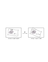
Figure 3: Inside the Riemannian constraint surface we consider a constraint orbit represented by $(A,E)_{deg}$ from (65). Therein the Wick rotation of non-degenerate representative $(A,E)$ from (70) shall be extended to its non-degenerate neighbourhood $\mathcal{U}(A,E)$. In the Lorentzian constraint surface ${\mathcal{U}}(\mathfrak{W}(A,E))$ will belong to the constraint orbit represented by $(A^{\prime},E^{\prime})_{deg}$, which can not be Wick rotated directly.

(ii) Let us now extend the point-wise Wick rotation of gauge fixed orbit representatives to their local non-degenerate neighbourhood in the associated constraint orbit. From local investigations in section VI.2 we know that our Wick rotation is a constraint preserving, symplectic isomorphism. Therefore it locally maps Riemannian phase-space flows generated by the constraints (i.e. gauge orbits) onto the Lorentzian ones. Hence we conclude that $\mathfrak{W}$ is locally compatible with non-degenerate parts of gauge orbits.

(iii) Consequently, connected non-degenerate part of a Riemannian gauge orbit will be mapped onto connected part of a corresponding Lorentzian gauge orbit.

If the set of non-degenerate points in a constraint orbit is simply connected, i.e. two non-degenerate points can always be connected by non-degenerate gauge trajectories, then all these points will be Wick rotated into the same Lorentzian constraint orbit. We would obtain a unique map from Riemannian to Lorentzian constraint orbits, by substitutional mapping of respective non-degenerate orbit representatives in part (i).

If the set of non-degenerate points in a Riemannian constraint orbit is not simply connected, then there are parts separated by degenerate boundary. The disconnected non-degenerate parts will be individually mapped into their respective Lorentzian constraint orbits. To obtain a global picture of the Wick rotated orbit, we have to incorporate degenerate points at the boundary of our non-degenerate parts for which $\mathfrak{W}$ is not defined and see what happens to our Wick rotation when we cross them. As discussed in Bruno thesis there the infinitesimal annihilation of dyad degeneracy in $(A,E)_{deg}$ to arbitrary $n^{I}\in(E^{I}_{deg})^{\perp}$ and its implications on the global continuity and orbit affiliation for our Wick rotation remain open problems.

VII Quantum Wick transform

The purpose of this section is to examine the action of the Wick transform operator constructed in section V. We will explicitly construct its action on elements of the Abelian Hilbert space $\mathcal{H}_{abel}\subset\mathcal{H}_{phys}$, on the measure on that space as well as on a complete set of operators which leave that space invariant. With respect to the identification of $\mathcal{H}_{abel}\simeq\mathcal{H}^{(red)}_{phys}$ with the (equivalent!) reduced phase space quantisation our results can formally be discussed as probing $\hat{\mathbf{W}}$ on physical states and physical observables. Even though the Wick operator provides the corresponding objects in the $SU(2)$ formulation of Lorentzian theory, we will see that, with the use of Wick rotation, we can naturally relate them to appropriate objects in $SU(1,1)$ formulation.

In order to evaluate the action of the Wick transform operator on a state (which is a function of flat abelian connection $A_{0}$) $\Psi^{E}(A_{0})\equiv\Psi^{E}(a_{1},a_{2})$, let us recall that in the Euclidean theory $a_{1},a_{2}\in(0,4\pi]$ parameterise a product of two circles $S^{1}\times S^{1}$. In the (spatial sector of) Lorentzian theory, a state is also a function of two real parameters. The difference is that now $a_{1},a_{2}\in\mathbb{R}^{2}$ and the state has the property that $\Psi(a_{1},a_{2})=\Psi(-a_{1},-a_{2})$. We can, however, equivalently regard the Euclidean functions as periodic functions on $\mathbb{R}^{2}$. This is what we will do from now on in order to be able to map Euclidean states to the Lorentzian ones. Therefore the Euclidean Hilbert space is now defined as the space of square integrable functions on a 2-torus: $\mathcal{H}^{E}=L^{2}(T^{2},{\rm d}\mu_{0})$, where the measure is given by ${\rm d}\mu_{0}:={\rm d}a_{1}\wedge{\rm d}a_{2}$. It is well known that such space is spanned by the basis which consists of functions $\sin(n_{1}a_{1}+n_{2}a_{2})$ and $\cos(m_{1}a_{1}+m_{2}a_{2})$, where $n_{I}$, $m_{I}$ ($I=1,2$) are arbitrary integers. Each of the basis elements is well defined not only for $(a_{1},a_{2})\in\mathbb{R}^{2}$, but also for arbitrary complex values of the two parameters. We will use this property to evaluate the action of the Wick transform operator on certain Euclidean states. We will use a dense subset of our Hilbert space $\mathcal{H}^{E}$ for explicit evaluation. The elements of the subset are finite linear combinations of $\sin$ and $\cos$ functions described above. For the rest of this section $\Psi^{E}$ denotes a function which belongs to this dense subset.

We can now make the following series expansion:

$$\Psi^{E}(a_{1},a_{2})=\sum_{n=0}^{\infty}\frac{1}{n!}a_{2}^{n}\partial_{2}^{n}\Psi^{E}(a_{1},0)$$ (77)

Using this series expansion (and the analogous one in the other variable), it is a straightforward calculation to show that:

$$\hat{\mathbf{W}}\Psi^{E}(a_{1},a_{2})={\rm e}^{i\frac{\pi}{2}}\Psi^{E}(ia_{1},ia_{2})$$ (78)

It is worth making an interesting observation here that multiplication of the flat connection by $i$ is precisely the action of the internal Wick rotation. Indeed, by construction we have $n_{I}A_{0}^{I}=0$. This also implies that $\mathfrak{W}(A_{0})$ belongs to the space-like sector of $SU(1,1)$ moduli space. It should be stressed here, that the above observation has been made for a very specific gauge fixed connection and we don’t know if it can be meaningfully extended to the whole gauge orbit. Let us nevertheless use this formal relation of the Wick transform with the Wick rotation to test its implications below. Thus, the state in the $SU(2)$ formulation of the Lorentzian theory is now defined as $\Psi(a_{1},a_{2})$ such that

$$\hat{\mathbf{W}}\Psi^{E}(a_{1},a_{2})=\Psi(a_{1},a_{2})$$ (79)

Note that (78) provides us with the following formal prescription for a construction of $\Psi$. Take a Euclidean solution $\Psi^{E}$, continue it analytically to complexified phase-space and evaluate it on the Wick rotated connection, i.e.

$$\Psi(A_{0})=\Psi^{E}(\mathfrak{W}(A_{0}))$$ (80)

Note that quantum Wick transform is described in terms of classical Wick rotation.

We can use it to map the restriction of physical observables to $\mathcal{H}_{abel}$ as proposed in Thiemann's W-paper ; Abhay's W-paper . As we know (see for example Abhay's Buch ) we can introduce the following, so called, loop variables which provide for us a complete set of observables:

$$T^{0}[\alpha](A):={\rm tr}h_{\alpha}(A)$$ (81)

$$T^{1}[\alpha](A,E):=\oint_{\alpha}ds^{a}\epsilon_{ab}{\rm tr}E^{b}h_{\alpha}(A)$$ (82)

Those variables are labeled by a loop $\alpha\subset\Sigma$, $h_{\alpha}$ denotes the holonomy around the loop and the trace is taken in the fundamental representation of the gauge group. When restricted to our reduced (Euclidean)phase-space

$$T^{0}[n_{1},n_{2}](a_{1},a_{2})=2\cos(a_{1}n_{1}+a_{2}n_{2})$$

where $n_{1}$, $n_{2}$ are winding numbers of the loop $\alpha$. From this, it is easy to show that

$$\hat{\mathbf{W}}\circ\hat{T}^{0}[n_{1},n_{2}](a_{1},a_{2})\circ\hat{\mathbf{W}}^{-1}=2\cosh(a_{1}n_{1}+a_{2}n_{2})$$ (83)

which is indeed equal to the operator $T^{0}$ evaluated on corresponding (through Wick rotation) $SU(1,1)$ connection. Similarly

$$T^{1}[n_{1},n_{2}](a_{1},a_{2},k_{1},k_{2})=2(k_{1}n_{2}-k_{2}n_{1})\sin(a_{1}n_{1}+a_{2}n_{2})$$

Using (80) one can then show that

$$\hat{\mathbf{W}}\circ\hat{T}^{1}[n_{1},n_{2}](a_{1},a_{2},k_{1},k_{2})\circ\hat{\mathbf{W}}^{-1}=2i\hbar\sinh(a_{1}n_{1}+a_{2}n_{2})n_{I}\epsilon_{IJ}\frac{\partial}{\partial a_{J}}$$ (84)

which, again agrees with the operator appearing in the Lorentzian $SU(1,1)$ theory.

In order to discuss the scalar product, recall that on our reduced quantum theory the appropriate product turns out to be Abhay's Buch $d\mu_{0}(A_{0})=da_{1}\wedge da_{2}$. Thiemann suggested in Thiemann's W-paper a strategy for constructing a scalar product on Wick transformed functions. The main condition for constructing such a product was to provide a distribution $\nu$ on complexified connections defined as:

$$\nu(A^{\mathbb{C}},\overline{A^{\mathbb{C}}})=\left(\left(\overline{\hat{\mathbf{W}}^{\dagger}}\right)^{\prime}\right)^{-1}\left(\overline{\left(\overline{\hat{\mathbf{W}}^{\dagger}}\right)^{\prime}}\right)^{-1}\delta(A^{\mathbb{C}},\overline{A^{\mathbb{C}}})$$ (85)

where bar denotes complex conjugation, prime denotes analytic continuation and the distribution $\delta$ is defined in Thiemann's W-paper (it reduces the integration over complex connections to integration over the real section $A^{\mathbb{C}}=\overline{A^{\mathbb{C}}}$). In our case of moduli space of flat connections we can evaluate $\nu$ explicitly. Using (78) we obtain:

$$\nu(A^{\mathbb{C}},\overline{A^{\mathbb{C}}})\equiv\nu(a_{I}^{\mathbb{C}},\overline{a_{J}^{\mathbb{C}}})=\delta(-ia_{I}^{\mathbb{C}},\overline{-ia_{J}^{\mathbb{C}}})$$ (86)

The result is therefore that, using our formal relation with Wick rotation, the measure provided by Thiemann’s construction restricts the integration over complex connections to the real section which is exactly the $SU(1,1)$ section defined by our Wick rotation. Furthermore, it reproduces the measure $da_{1}\wedge da_{2}$ in which the Lorentzian observables $\hat{T}^{0}$ and $\hat{T}^{1}$ are self-adjoint.

Finally, we would like to ask if the Wick transform provides for us sufficiently many Lorentzian states to be at all interesting. If we look at the basis in $\mathcal{H}^{E}$ given by sin and cos functions as above, the answer is not obvious. The reason for this is that the Wick transform acting on any such basis element produces a sinh or cosh function. The first of those does not belong to the Lorentzian physical Hilbert space $\mathcal{H}^{L}$ and the second one is not normalisable on the real line. Let us consider, however, a different subset of $\mathcal{H}^{E}$

$$\Psi^{E}_{n_{1},n_{2}}(a_{1},a_{2})=f_{n_{1}}^{E}(a_{1})f_{n_{2}}^{E}(a_{2})+f_{n_{1}}^{E}(-a_{1})f_{n_{2}}^{E}(-a_{2})$$ (87)

where $n_{1},n_{2}=0,1,2,3,\ldots$ and

$$f_{n}^{E}(a):=e^{(2n+1)ia}\exp(-\frac{1}{2}e^{2ia})$$ (88)

It is easy to see that under the Wick transform each function $f_{n}^{E}(a)$ is mapped to

$$f_{n}(a):=\hat{\mathbf{W}}f_{n}^{E}(a)=e^{-(2n+1)a}\exp(-\frac{1}{2}e^{-2a})$$ (89)

Since the result dies out (at least) exponentially when $a\rightarrow\pm\infty$, we obtain an element of the Lorentzian Hilbert space. In fact, we will show that in this way we obtain a dense subset of $\mathcal{H}^{L}$. In order to do that, let us consider a family of functions $g_{n}(x):=x^{n}e^{-\frac{1}{2}x}$, where $x\in\mathbb{R}_{+}$ ($x$ is a positive real number). It is well known that this is a complete set of functions in $L^{2}(\mathbb{R}_{+},dx)$. By making the substitution $x=e^{-2a}$ we obtain functions on the real line $g_{n}(a)=e^{-2na}\exp(-\frac{1}{2}e^{-2a})$. These form a complete set in $L^{2}(\mathbb{R},e^{-2a}da)$. This, in turn, implies that $f_{n}(a)=e^{-a}g_{n}(a)$ is a complete set in $L^{2}(\mathbb{R},da)$. Finally, it is easy to see that the following set is complete in the Lorentzian Hilbert space:

$$\Psi_{n_{1},n_{2}}(a_{1},a_{2})=f_{n_{1}}(a_{1})f_{n_{2}}(a_{2})+f_{n_{1}}(-a_{1})f_{n_{2}}(-a_{2})$$ (90)

Thus, we have shown that the quantum Wick transform is able to reproduce all states of the Lorentzian theory (at least in this limited context of $\mathcal{H}_{abel}$ in 2+1 gravity). Notice that this is not a trivial statement, since the Wick transform is not an isomorphism! Therefore, a priori, it was not known if it provides sufficiently many (or any) Lorentzian states.

VIII Conclusions

The generalised Wick transform quantisation method Thiemann's W-paper ; Abhay's W-paper is an attractive strategy to simplify the appearance of the last and the key step in the canonical quantisation program for general relativity, namely solving the scalar constraint $\hat{\mathcal{S}}_{L}$. In full quantum theory it has remained formal. The main motivation behind this paper is to use simpler truncated models to test if the program can be made rigorous and to gain insight into the resulting physical states. Along with these efforts there are three natural ways to implement the basic Wick transform construction principle of employing internal isomorphisms in the complexified phase space to relate simpler Riemannian theory with physical Lorentzian quantum theory:

(i) the usual Wick transform relates different appearances of the same Lorentzian theory, where we formally recover simpler Riemannian constraints however subject to complicated reality conditions.

(ii) in the generalised Wick transform the previous concept is lifted to the algebra of functions on the common real phase space of both theories, thus providing a genuine map from real Riemannian to real Lorentzian quantum theory.

(iii) the Wick rotation is particularly adapted to the simpler framework of $2+1$ gravity and employs a phase space isomorphism between embeddings of both real theories into the complexified phase space. In contrast to (i) it is a genuine phase space map from Riemannian to Lorentzian classical general relativity and naturally avoids reality conditions.

Our main emphasis is to test the particular quantisation program which arises from the generalised Wick transform, in order to explore associated subtleties which are expected to arise similarly when applied to full quantum gravity. On Bianchi models the reduced Wick transform strategy can be implemented in detail and is shown to reproduce the identical quantum theory as obtained from Dirac quantisation. Furthermore we explicitly observed for Bianchi type I, that to obtain physical states from quantum Wick transform, one has to restrict the Hilbert space of Riemannian quantum theory to states which are subject to additional boundary conditions.

We investigate different connection dynamical formulations of classical 2+1 dimensional general relativity and recover among others the analog for the generalised Wick transform therein. The corresponding Wick transform operator $\mathbf{\hat{W}}$ causes similar regularisation problems as in full gravity. Its restriction to a small subspace of Riemannian quantum theory allows to study the operators explicitly and glimpses to the same behaviour as on Bianchi models. However it does not provide a full understanding for the quantum Wick transform and the resulting physical states in $2+1$ gravity. This is achieved by testing the Wick transform quantisation indirectly in an appearance which classically arises from the internal Wick rotation. Here we relate standard Riemannian theory to the simpler $\mathfrak{su}(1,1)$ formulation of Lorentzian $2+1$ theory. When induced to the reduced phase space this Wick transform provides a natural map from solutions of Riemannian quantum theory to physical states of Lorentzian quantum theory, however now expressed in the simpler $\mathfrak{su}(1,1)$ formulation. Our Wick rotation is a preliminary technique in $2+1$ gravity for our main object of interest the generalised Wick transform $\mathbf{\hat{W}}$. As presently formulated it can not be used to regularise $\mathbf{\hat{W}}$ geometrically, however it allows to characterise the resulting physical states. In the case of space-time topology $M^{2,1}\cong T^{2}\times\mathbb{R}$ we study the resulting physical states explicitly and observe that the Wick transform leads us to the most interesting, space-like sector of $2+1$ gravity.

Fianlly, let us mention that the work done in section VII can easily be extended to the $2+1$ gravity with a non-vanishing cosmological constant. It is easy to check that Wick rotation and Wick transform have the same properties when $\Lambda\neq 0$. Furthermore, Ezawa has provided reduced phase-space representatives in Ezawa . As before, they can be chosen to be constant Abelian elements of the phase-space. Because of that, the analysis of the section VII can be performed without virtually any changes for arbitrary $\Lambda$.

*

Appendix A Differential geometry of the phase space variables

To understand the subtleties of our internal Wick rotation we reflect the phase space variables from the perspective of differential geometry Nakahara . Their transparent geometrical nature is usually hidden behind the coordinate dependent terminology utilized in physics.

The mathematical space which carries all phase space variables of connection dynamics is an adjoint vector bundle $P\times_{Ad}\mathfrak{g}$, which is associated with a $P(\Sigma,G)$ principal bundle. In our case $\mathfrak{g}$ is the Lie algebra of $SU(2)$ or $SU(1,1)$. The dyads $E^{I}_{a}$ represent sections in the adjoint bundle $Ad\>P:=P\times_{Ad}\mathfrak{g}$ and the connection $1$-forms $A^{I}_{a}$ are closely related to covariant derivatives $\partial^{(Z)}$ thereon.

On a principal fibre bundle $P$ a connection $Z\in\mathcal{C}(P)$ is a unique smooth right-invariant separation of the tangent space $TP$ into vertical and horizontal subspace. Such a connection can be described in terms of a $\mathfrak{g}$-valued $1$-form $Z\in\Omega^{1}_{Ad}(P,\mathfrak{g})$ with the following requirements:

$$(i)\; Z(\tilde{X})=X\;\;\;\;\;\;X\in\mathfrak{g}$$

$$(ii)\; R^{\ast}_{g}Z=Ad_{g^{-1}}Z$$

By adding a $1$-form $\overline{A}\in\overline{\Omega}^{1}_{Ad}(P,\mathfrak{g})$, which is tensorial (vanishes on vertical vector fields) and of type $Ad$ (under right-multiplication with $G$) to a given connection $Z_{1}$ we obtain another connection $Z_{2}:=Z_{1}+\overline{A}$. This makes the space of all connections $\mathcal{C}(P)$ an affine space with the vector space $\overline{\Omega}^{1}_{Ad}(P,\mathfrak{g})$. Further every connection $Z$ uniquely defines an absolute differential $D^{Z}:=d\circ\pi_{horiz}:\overline{\Omega}^{k}_{Ad}(P,\mathfrak{g})\rightarrow\overline{\Omega}^{k+1}_{Ad}(P,\mathfrak{g})$, which satisfies:

$$D^{Z}\overline{\omega}:=d\overline{\omega}+Ad_{\ast}(Z)\wedge\overline{\omega}$$ (91)

Our phase space variables act on the associated vector bundle $Ad\>P:=P\times_{Ad}\mathfrak{g}$. There exists a canonical isomorphism:

$$\overline{\Omega}^{k}_{Ad}(P,\mathfrak{g}) \tilde{\longrightarrow} \Omega^{k}(\Sigma,Ad\>P)$$

$$\overline{\omega} \longmapsto \omega:=[s,s^{\ast}\overline{\omega}]$$ (92)

where $[s,s^{\ast}\overline{\omega}]$ denotes the (gauge) equivalence class in $Ad\>P$ which is obtained by choosing an arbitrary section $s\in P$ and pulling back $\overline{\omega}$ from $P$ to $\Sigma$. For every connection $Z\in\mathcal{C}(P)$ this isomorphism induces the absolute differential to a unique covariant derivative $\partial^{Z}$ on the associated vector bundle, which is defined on sections $[s,s^{\ast}\overline{\omega}]\in\Omega^{0}(\Sigma,Ad\>P)$ as:

$$\partial^{Z}\omega(X):=[s,s^{\ast}D^{Z}\overline{\omega}\>(X)]=[s,d\overline{\omega}(dsX)+Ad_{\ast}(Z(dsX))\wedge\overline{\omega}\circ s]$$ (93)

In particular for an arbitrary element $Z+\overline{A}$ in the affine space of connections the corresponding unique element $\partial^{Z+\overline{A}}$ in the affine space of covariant derivatives can be parameterised in terms of $1$-forms $A\in\Omega^{1}(\Sigma,Ad\>P)$ and a fixed covariant derivative $\partial^{Z}$:

$$\partial^{Z+\overline{A}}\omega(X)=\partial^{Z}\omega(X)+[s,Ad_{\ast}(s^{\ast}A(X))\wedge\overline{\omega}\circ s]$$ (94)

Let us now recover our phase space variables in the more coordinate dependent terminology in physics. All differential forms in the associated vector bundle in (92) are equivalence classes and therefore defined depending on an arbitrary section $s:\Sigma\rightarrow P$ in the principal bundle, which is called gauge. From now on we assume a fixed gauge $s$ in $P$. The pull back $s^{\ast}\overline{\omega}$ of $\overline{\omega}\in\overline{\Omega}^{k}_{Ad}(P,\mathfrak{g})$ is a Lie-algebra valued k-form on the base manifold $\Sigma$. Following these definitions all sections $\omega$ in (93) will be described in terms of a $\mathfrak{g}$ valued function $\omega^{I}:=\overline{\omega}\circ s$, pull backs of connection $1$-forms $Z\in\mathcal{C}(P)$ in (93) will appear as $\mathfrak{g}$ valued $1$-forms $Z^{I}_{a}:=s^{\ast}Z$ and pulled back vector space elements $s^{\ast}A$ in (94) from the affine space of connections will appear as $\mathfrak{g}$ valued $1$-forms $A^{I}_{a}:=s^{\ast}\overline{A}$. The adjoint representation on the Lie algebra is nothing else than the commutator $Ad_{\ast}A:=[A,\cdot]$ for $A\in\mathfrak{g}$. Let us furthermore note, that all covariant derivatives in the adjoint bundle $P\times_{Ad}\mathfrak{g}$ are naturally compatible with $\eta_{IJ}$, which is induced from the $Ad$-invariant Cartan-Killing metric on $\mathfrak{g}$.

The resulting formulation arises from suppressing the gauge in the associated vector bundle formalism and from applying the above abstract index notation. Following these lines the affine space of all connections - i.e. the space of all covariant derivatives (94) - can be parameterised by:

$$\partial^{(Z+\overline{A})}_{a} = \underbrace{\partial_{a}+Ad_{\ast}(Z^{I}_{a})}+Ad_{\ast}(A^{I}_{a})$$

$$= \;\;\;\;\;\;\;\;\partial^{(Z)}_{a}\;\;\;\;\;\;\,+\varepsilon^{I}_{JK}(A^{J}_{a})$$

In particular its parameterization in terms of connection $1$-forms $A^{i}_{a}$ makes only sense with respect to an once and for all fixed connection $Z^{I}_{a}$ - i.e. fixed reference covariant derivative $\partial^{(Z)}_{a}$.

In the proposed internal Wick rotation (section VI.1) the dyad component of the phase space variables $(E,A)$ will determine how to map the connection. In our parameterisation of the affine space of connections this will be realised by simultaneously mapping connection $1$-forms $A^{I}_{a}$ and their reference covariant derivative $\partial_{a}$. For that purpose we choose the reference $\partial_{a}$ in a way, which allows us to identify $\overline{\partial}_{a}:=\partial_{a}^{\mathfrak{sl}(2,\mathbb{C})}|_{\mathfrak{W}(\mathfrak{su}(2))}$ as a suitable $\mathfrak{su}(1,1)$ covariant derivative. This can be achieved with every flat covariant derivative $\tilde{\partial}_{a}$ which is compatible with the normal $\tilde{\partial}_{a}n^{I}=0$ (and with $\eta_{IJ}$ anyway). Then, by canonically extending $\tilde{\partial}_{a}$ to the real $6$-dimensional $\mathfrak{sl}(2,\mathbb{C})$ vector bundle its restriction $\overline{\tilde{\partial}}_{a}:=\tilde{\partial}_{a}^{\mathfrak{sl}(2,\mathbb{C})}|_{\mathfrak{W}(\mathfrak{su}(2))}$ is again flat. We notice that $\overline{\tilde{\partial}}_{a}\;i\cdot u_{\perp}=i\cdot\tilde{\partial}_{a}u_{\perp}$. For every non-degenerate dyad $E^{I}_{a}$ such a $\tilde{\partial}_{a}$ can be defined from extending $n^{I}$ to a basis of parallel sections in the vector bundle.

References

- (1) C. Rovelli, Notes for a brief history of quantum gravity, gr-qc/0006061 (2001)
- (2) A. Ashtekar, Lectures on Non-perturbative Canonical Gravity, Notes prepared in collaboration with R. S. Tate, World Scientific, Singapore (1991)
- (3) T. Thiemann, Reality conditions inducing transforms for quantum gauge field theory and quantum gravity, Class. Quantum Grav. 13 1383-1404 (1996)
- (4) A. Ashtekar, A generalized Wick transform for Gravity, Phys. Rev. D 53 2865-2869 (1996)
- (5) B. Hartmann, Generalized Wick Transform in Dimensionally Reduced Gravity, diploma thesis, Humboldt University Berlin, Preprint SFB 288 No.582 (2002)
- (6) A. Ashtekar, R. Tate, C. Uggla, Minisuperspaces: Observables and Quantization, Int. J. Mod. Phys. D 2 15-50 (1993)
- (7) J. D. Romano, Geometrodynamics versus Connection Dynamics, Gen. Rel. Grav. 25 759-854 (1993)
- (8) J. Wiśniewski, 2+1 general relativity: classical and quantum, Ph.D. thesis, The Pennsylvania State University (2002)
- (9) J. F. Barbero G., Real Ashtekar Variables for Lorentzian Signature Space-times, Phys. Rev. D 51 5507-5510 (1995)
- (10) J. Louko and D. M. Marolf, Solution space of gravity on in Witten’s connection formulation, Class. Quantum Grav. 11 311-330 (1994)
- (11) E. Witten, dimensional gravity as an exactly soluble system, Nucl. Phys. B311 46-78 (1988/89)
- (12) K. Ezawa, Classical and quantum evolutions of the de Sitter and the anti-de Sitter universes in dimensions, Phys. Rev. D 49 5211-5226 (1994)
- (13) M. Nakahara, Geometry, topology and physics, Adam Hilger, Bristol and New York (1990)