Field propagation in de Sitter black holes

Abstract

We present an exhaustive analysis of scalar, electromagnetic and gravitational perturbations in the background of Schwarzchild–de Sitter and Reissner–Nordström–de Sitter spacetimes. The field propagation is considered by means of a semi–analytical (WKB) approach and two numerical schemes: the characteristic and general initial value integrations. The results are compared near the extreme cosmological constant regime, where analytical results are presented. A unifying picture is established for the dynamics of different spin fields.

I Introduction

Wave propagation around nontrivial solutions of Einstein equations, black holes in particular, is an active field of research (see Regge-57 ; Chandrasekhar ; Kokkotas-99 and references therein). The perspective of gravitational wave detection in the near future and the great development of numerical general relativity have increased even further the activity on this field. Gravitational waves should be especially strong when emitted by black holes. The study of the propagation of perturbations around them is, hence, essential to provide templates for gravitational wave identification. On the other hand, recent astrophysical observations indicate that the universe is undergoing an accelerated expansion phase, suggesting the existence of a small positive cosmological constant and that de Sitter (dS) geometry provides a good description of very large scales of the universe accel-exp . We notice also that string theory has recently motivated many works on asymptotically anti–de Sitter spacetimes (see, for instance, Cardoso-01 ; AdS-4d ; AdS-other ; Wang-01 ).

In this work, we perform an exhaustive investigation of scalar, electromagnetic, and gravitational perturbations in the background of Schwarzchild–de Sitter (SdS) and Reissner–Nordström–de Sitter (RNdS) spacetimes. Contrasting with the noncharged case, in the RNdS one the electromagnetic and gravitational perturbations are necessarily coupled. We scan the full range of the cosmological constant, from the asymptotic flat case ($\Lambda=0$) up to the critical value of $\Lambda$ which characterizes, for the noncharged case, the Nariai solution Nariai . Two different numerical methods and a higher order WKB analysis are used. The results are compared near the extreme $\Lambda$ regime, where analytical results can be obtained.

We recall that for any perturbation in the spacetimes we consider that, after the initial transient phase, there are two main contributions to the resulting asymptotic wave Leaver-86 ; Ching-95 : initially the so-called quasinormal modes, which are suppressed at later time by the tails. The first can be understood as candidates for normal modes which, however, decay (their energy eigenvalues becomes complex), as in the ingenious mechanism first described by Gamow in the context of nuclear physics Gamow-28 . After the initial transient phase, the properties of the resulting waves are more related to the background spacetime rather than to the source itself.

It is well known that for asymptotically flat backgrounds the tails decay according to a power law, whereas in a space with a positive cosmological constant the decay is exponential. Curiously, $\ell=0$ modes for scalar fields in dS spacetimes, contrasting with the asymptotic flat cases, exponentially approach a nonvanishing asymptotic value Brady-97 ; Brady-99 . We detected, by using a noncharacteristic numerical integration scheme, a dependence of this asymptotic value on the initial velocities. In particular, it vanishes for static initial conditions. Our results are in perfect agreement with the analytical predictions of Brady-99 .

The semianalytical analyses of this work were performed by using the higher order WKB method proposed by Schutz and Will Schutz-85 , and improved by Iyer and Will Iyer-87 ; WKB-ap . It provides a very accurate and systematic way to study black hole quasinormal modes. We apply it to the study of various perturbation fields in the nonasymptotically flat dS geometry. Quasinormal modes are also calculated according to this approximation, and the results are compared to the numerical ones whenever appropriate, providing a quite complete picture of the question of quasinormal perturbations for dS black holes.

Concerning the charged case, we analyze in detail the wave propagation of the massless scalar field and coupled electromagnetic and gravitational fields in the RNdS spacetime. An important difference concerning the dynamics of the electromagnetic and gravitational fields is that there are no pure modes, since both are interrelated. We will show that the direct picture of the evolution presents us with perfect agreement of quasinormal frequencies with those obtained by using the approximation method suggested in Schutz-85 ; Iyer-87 . One important point assessed is the dependence of the fields’ decay on the electric charge of the black hole, including the asymptotically flat limit, for which we expected to find traces of a power law tail appearing between the quasinormal modes and the exponential tail.

Two very recent works overlap our analysis presented here. A similar WKB approach, presented in Konoplya-03 , was used very recently by Zhidenko Zhidenko to study SdS black holes, giving results in agreement with ours. Yoshida and Futamase Yoshida used a continued fraction numerical code to calculate quasinormal mode frequencies, with special emphasis on high order modes. Our results are also compatible. Finally, we notice that solutions of the wave equation in a nontrivial background have also been used to infer intrinsic properties of the spacetime qnmbh .

The paper is organized as follows. Sec. II provides theoretical considerations and reviews some well-known results that were useful to our work; Sec. III briefly explains the numerical and semianalytical methods employed, followed by Sec. IV, which presents, in detail, our results on field dynamics for near extreme SdS and RNdS geometries. Sec. V deals with the so-called intermediary region, where the geometries are not extreme. Data on the SdS limit and on exponential tails are also presented. Sec. VI deals with the near asymptotically flat region, and Sec. VII presents our conclusions.

II Metric, fields, and effective potentials

The metric describing a charged, asymptotically de Sitter spherical black hole, written in spherical coordinates, is given by

$$ds^{2}=-h(r)dt^{2}+h(r)^{-1}dr^{2}+r^{2}(d\theta^{2}+\sin^{2}\theta d\phi^{2})\ ,$$ (1)

where the function $h(r)$ is

$$h(r)=1-\frac{2m}{r}+\frac{q^{2}}{r^{2}}-\frac{\Lambda r^{2}}{3}\ .$$ (2)

The integration constants $m$ and $q$ are the black hole mass and electric charge, respectively. If the cosmological constant is positive, we have the Reissner–Nordström–de Sitter metric. In this case, $\Lambda$ is usually written as $\Lambda=3/a^{2}$, where the constant $a$ is the “cosmological radius.”

The spacetime causal structure depends strongly on the zeros of $h(r)$. Depending on the parameters $m$, $q$, and $a$, the function $h(r)$ may have three, two, or even no real positive zeros. For the RNdS cases we are interested in, $h(r)$ has three simple real, positive roots ($r_{c}$, $r_{+}$, and $r_{-}$), and a real and negative root $r_{n}=-(r_{-}+r_{+}+r_{c})$. The horizons $r_{-}$, $r_{+}$, and $r_{c}$, with $r_{-}<r_{+}<r_{c}$, are denoted Cauchy, event, and cosmological horizons, respectively.

For the SdS case ($q=0$), and assuming $m>0$ and $0<9m^{2}\Lambda<1$, the function $h(r)$ has two positive zeros $r_{+}$ and $r_{c}$ and a negative zero $r_{n}=-(r_{+}+r_{c})$. This is the SdS geometry in which we are interested. The horizons $r_{+}$ and $r_{c}$, with $r_{+}<r_{c}$, are denoted the event and cosmological horizons, respectively. In this case, the constants $m$ and $a$ are related to the roots by

$$a^{2}=r_{+}^{2}+r_{c}^{2}+r_{+}r_{c}\ ,$$ (3)

$$2ma^{2}=r_{+}r_{c}(r_{+}+r_{c})\ .$$ (4)

If $9m^{2}\Lambda=1$, the zeros $r_{+}$ and $r_{c}$ degenerate into a double root. This is the extreme SdS black hole. If $m^{2}\Lambda>1$, there are no real positive zeros, and the metric (1) does not describe a black hole.

In both the SdS and RNdS cases, we shall study the perturbation fields in the exterior region, defined as

$$T_{+}=\left\{(t,r,\theta,\phi),r_{+}<r<r_{c}\right\}\ .$$ (5)

In this region $T_{+}$, we define a “tortoise coordinate” $x(r)$ in the usual way,

$$x(r) = -\frac{1}{2\kappa_{c}}\ln(r_{c}-r)+\frac{1}{2\kappa_{+}}\ln(r-r_{+})$$ (6)

$$\mbox{}-\frac{1}{2\kappa_{-}}\ln(r-r_{-})+\frac{1}{2\kappa_{n}}\ln(r-r_{n})\ ,$$

with

$$\kappa_{i}=\frac{1}{2}\left|\frac{dh(r)}{dr}\right|_{r=r_{i}}\ .$$ (7)

The constants $\kappa_{-}$, $\kappa_{+}$, and $\kappa_{c}$ are the surface gravities associated with the Cauchy, event, and cosmological horizons, respectively. For the SdS case, the term associated with the Cauchy horizon is absent.

Consider now a scalar perturbation field $\Phi$ obeying the massless Klein-Gordon equation

$$\Box\Phi=0\ .$$ (8)

The usual separation of variables in terms of a radial field and a spherical harmonic $\textrm{Y}_{\ell,m}(\theta,\varphi)$,

$$\Phi=\sum_{\ell\,m}\frac{1}{r}\psi_{\ell}^{sc}(t,r)\textrm{Y}_{\ell}(\theta,\phi)\ ,$$ (9)

leads to Schrödinger-type equations in the tortoise coordinate for each value of $\ell$,

$$-\frac{\partial^{2}\psi_{\ell}^{sc}}{\partial t^{2}}+\frac{\partial^{2}\psi_{\ell}^{sc}}{\partial x^{2}}=V^{sc}(x)\psi_{\ell}\ ,$$ (10)

where the effective potential $V^{sc}$ is given by

$$V^{sc}(r)=h(r)\left[\frac{\ell(\ell+1)}{r^{2}}+\frac{2m}{r^{3}}-\frac{2q^{2}}{r^{4}}-\frac{2}{a^{2}}\right]\ .$$ (11)

The situation for higher spin perturbations is quite different. In the SdS geometry, in contrast to the case of an electrically charged black hole, it is possible to have pure electromagnetic and gravitational perturbations. For both cases, we have Schrödinger-type effective equations. For the first, the effective potential is given by Ruffini-72

$$V^{el}(r)=h(r)\frac{\ell(\ell+1)}{r^{2}},$$ (12)

with $\ell\geq 1$. The gravitational perturbation theory for the exterior Schwarzschild–de Sitter geometry has been developed in Chandrasekhar ; Cardoso-01 . The potentials for the axial and polar modes are, respectively,

$$V^{ax}(r)=h(r)\left[\frac{\ell(\ell+1)}{r^{2}}-\frac{6m}{r^{3}}\right]\ ,$$ (13)

$$V^{po}(r) = \frac{2h(r)}{r^{3}\left(3m+cr\right)^{2}}\left[9m^{3}+3c^{2}mr^{2}+c^{2}(1+c)r^{3}\right.$$ (14)

$$\mbox{}\left.+3m^{2}(3cr-\Lambda r^{3})\right]\ ,$$

with $2c=(\ell-1)(\ell+2)$ and $\ell\geq 2$. For perturbations with $\ell>0$, we can show explicitly that all the effective potentials $V(x)\equiv V(r(x))$ are positive definite. For scalar perturbations with $\ell=0$, however, the effective potential has one zero point $x_{0}$ and it is negative for $x>x_{0}$.

The perturbation theory for the RNdS geometry has been developed in Mellor-90 . There are neither purely electromagnetic nor gravitational modes. Indeed, we have four mixed electromagnetic and gravitational fields, two of them called polar fields, $Z_{1}^{+}$ and $Z_{2}^{+}$ (since they impart no rotation to the black hole) and two named axial fields, $Z_{1}^{-}$ and $Z_{2}^{-}$. It is possible to express their dynamics in four decoupled wave equations, two for the axial fields and two for the polar fields. Their deduction can be found in Mellor-90 and references therein. Here we just show the expressions, which will be useful throughout our work.

The axial perturbations $Z_{1,2}^{-}$ are governed by wave equations which have the same form as Eq. (10), but with effective potentials given by

$$V_{1}^{-}=h(r)\left[\frac{\ell(\ell+1)}{r^{2}}+\frac{4q^{2}}{r^{2}}-\frac{3m-\sqrt{9m^{2}+8cq^{2}}}{r^{3}}\right]\ ,$$ (15)

$$V_{2}^{-}=h(r)\left[\frac{\ell(\ell+1)}{r^{2}}+\frac{4q^{2}}{r^{2}}-\frac{3m+\sqrt{9m^{2}+8cq^{2}}}{r^{3}}\right]\ ,$$ (16)

respectively, with $2c=(\ell-1)(\ell+2)$.

The polar perturbations $Z_{1,2}^{+}$ are subjected to rather cumbersome potentials, as we can see below:

$$V_{1}^{+}=\frac{h(r)}{r^{3}}\left[U+\frac{1}{2}(p_{1}-p_{2})W\right]\ ,$$ (17)

$$V_{2}^{+}=\frac{h(r)}{r^{3}}\left[U-\frac{1}{2}(p_{1}-p_{2})W\right]\ ,$$ (18)

$$p_{1}=3m+\sqrt{9m^{2}+8cq^{2}}\ ,$$ (19)

$$p_{2}=3m-\sqrt{9m^{2}+8cq^{2}}\ ,$$ (20)

$$W=\frac{rh(r)}{\bar{\omega}^{2}}(2cr+3m)+\frac{1}{\bar{\omega}}\left(cr+m+\frac{2}{3}\Lambda r^{3}\right)\ ,$$ (21)

$$U=(2cr+3m)W+\left(\bar{\omega}-cr-m-\frac{2}{3}\Lambda r^{3}\right)-\frac{2cr^{2}h(r)}{\bar{\omega}}\ ,$$ (22)

$$\bar{\omega}=cr+3m-\frac{2q^{2}}{r}\ .$$ (23)

In the limit $q\rightarrow 0$, the RNdS potentials $V_{2}^{\pm}$ go into the SdS polar and axial potentials, $V^{\pm}$. Therefore, the minimum $\ell$ for these fields is $\ell=2$, while the $V_{1}^{\pm}$ fields admit $\ell=1$ as their minimum $\ell$ value, since they become electromagnetic perturbations in the limit $q\rightarrow 0$.

III Numerical and semianalytical approaches

III.1 Characteristic integration

In Gundlach-94 a simple but at the same time very efficient way of dealing with two-dimensional d’Alembertians has been set up. Along the general lines of the pioneering work Price-72 , the authors introduced light-cone variables $u=t-x$ and $v=t+x$, in terms of which all the wave equations introduced have the same form. We call $V$ the generic effective potential and $\psi_{\ell}$ the generic field, and the equations can be written, in terms of the null coordinates, as

$$-4\frac{\partial^{2}}{\partial u\partial v}\psi_{\ell}(u,v)=V(r(u,v))\psi_{\ell}(u,v)\ .$$ (24)

In the characteristic initial value problem, initial data are specified on the two null surfaces $u=u_{0}$ and $v=v_{0}$. Since the basic aspects of the field decay are independent of the initial conditions (this fact is confirmed by our simulations), we use

$$\psi_{\ell}(u=u_{0},v)=\exp\left[-\frac{(v-v_{c})^{2}}{2\sigma^{2}}\right]\ ,$$ (25)

$$\psi_{\ell}(u,v=v_{0})=\exp\left[-\frac{(v_{0}-v_{c})^{2}}{2\sigma^{2}}\right].$$ (26)

Due to the size of our lattices, the latter constant can be set to zero for any practical purpose.

Since we do not have analytic solutions to the time-dependent wave equation with the effective potentials introduced, one approach is to discretize Eq. (24) and then implement a finite differencing scheme to solve it numerically. One possible discretization, used, for example, in Wang-01 ; Brady-97 ; Brady-99 , is

$$\psi_{\ell}(N)=\psi_{\ell}(W)+\psi_{\ell}(E)-\psi_{\ell}(S)$$ (27)

$$\mbox{}-\Delta^{2}V(S)\frac{\psi_{\ell}(W)+\psi_{\ell}(E)}{8}+O(\Delta^{4})\ ,$$

where we have used the definitions for the points $N=(u+\Delta,v+\Delta)$, $W=(u+\Delta,v)$, $E=(u,v+\Delta)$, and $S=(u,v)$. With the use of expression (27), the basic algorithm will cover the region of interest in the $u-v$ plane, using the value of the field at three points in order to compute it at a fourth.

After the integration is completed, the values $\psi_{\ell}(u_{max},v)$ and $\psi_{\ell}(u,v_{max})$ are extracted, where $u_{max}$ ($v_{max}$) is the maximum value of $u$ ($v$) on the numerical grid. Taking sufficiently large $u_{max}$ and $v_{max}$, we have good approximations for the wave function at the event and cosmological horizons.

III.2 Noncharacteristic integration

It is not difficult to set up a numeric algorithm to solve Eq. (10) with Cauchy data specified on a $t$ constant surface. We used a fourth order in $x$ and a second order in $t$ scheme (see, for instance, Levander for an application of this algorithm to seismic analysis). The second spatial derivative at a point $(t,x)$, up to fourth order, is given by

$$\psi_{\ell}^{\prime\prime}(t,x) = \frac{1}{12\Delta x^{2}}\left[\psi_{\ell}(t,x+2\Delta x)-16\psi_{\ell}(t,x+\Delta x)\right.$$ (28)

$$\mbox{}+30\psi_{\ell}(t,x)-16\psi_{\ell}(t,x-\Delta x)$$

$$\left.+\psi_{\ell}(t,x-2\Delta x)\right]\ ,$$

while the second time derivative up to second order is

$$\ddot{\psi}_{\ell}(t,x)=\frac{\psi_{\ell}(t+\Delta t,x)-2\psi_{\ell}(t,x)+\psi_{\ell}(t-\Delta t,x)}{\Delta t^{2}}\ .$$ (29)

Given $\psi_{\ell}(t=t_{0},x)$ and $\psi_{\ell}=(t=t_{0}-\Delta t,x)$ (or $\dot{\psi}_{\ell}(t=t_{0},x)$), we can use the discretization in Eqs. (28) and (29) to solve Eq. (10) and calculate $\psi_{\ell}(t=t_{0}+\Delta t,x)$. This is the basic algorithm. At each interaction, one can control the error by using the invariant integral (the wave energy) associated with Eq. (10)

$$E=\frac{1}{2}\int\left[\left(\psi_{\ell}^{\prime}(t,x)\right)^{2}+\left(\dot{\psi}_{\ell}(t,x)\right)^{2}+V(x)\psi_{\ell}(t,x)^{2}\right]\,dx\ .$$ (30)

We make an exhaustive analysis of the asymptotic behavior of the solutions of Eq. (10) with initial conditions of the form

$$\psi_{\ell}(0,x)=\exp\left[-\frac{(x-x_{0})^{2}}{2\sigma_{0}^{2}}\right]\ ,$$ (31)

$$\dot{\psi}_{\ell}(0,x)=A\exp\left[-\frac{(x-x_{1})^{2}}{2\sigma_{1}^{2}}\right]\ .$$ (32)

The results do not depend on the details of the initial conditions. They are compatible with the ones obtained by the usual characteristic integration, with the only, and significant, exception of the $\ell=0$ scalar mode. As we will see, its asymptotic value depends strongly on the initial velocities $\dot{\psi}_{\ell}(0,x)$, a behavior already advanced in the work Brady-99 .

III.3 WKB analysis

Considering the Laplace transform of Eq. (10), one gets the ordinary differential equation

$$\frac{d^{2}\psi_{\ell}(x)}{dx^{2}}-\left[s^{2}+V(x)\right]\psi_{\ell}(x)=0\ .$$ (33)

One finds that there is a discrete set of possible values for $s$ such that the function $\hat{\psi}_{\ell}$, the Laplace-transformed field, satisfies both boundary conditions,

$$\lim_{x\rightarrow-\infty}\hat{\psi}_{\ell}\,e^{sx}=1\ ,$$ (34)

$$\lim_{x\rightarrow+\infty}\hat{\psi}_{\ell}\,e^{-sx}=1\ .$$ (35)

By making the formal replacement $s=i\omega$, we have the usual quasinormal mode boundary conditions. The frequencies $\omega$ (or $s$) are called quasinormal frequencies.

The semianalytic approach used in this work Schutz-85 ; Iyer-87 is a very efficient algorithm to calculate the quasinormal frequencies, which have been applied in a variety of situations WKB-ap . With this method, the quasinormal modes are given by

$$\omega_{n}^{2}=\left(V_{0}+P\right)-i\left(n+\frac{1}{2}\right)\left(-2V_{0}^{(2)}\right)^{1/2}\left(1+Q\right)$$ (36)

where the quantities $P$ and $Q$ are determined using

$$P=\frac{1}{8}\left[\frac{V_{0}^{(4)}}{V_{0}^{(2)}}\right]\left(\frac{1}{4}+\alpha^{2}\right)-\frac{1}{288}\left[\frac{V_{0}^{(3)}}{V_{0}^{(2)}}\right]^{2}\left(7+60\alpha^{2}\right)\ ,$$ (37)

$$Q = \frac{1}{-2V_{0}^{(2)}}\left\{\frac{5}{6912}\left[\frac{V_{0}^{(3)}}{V_{0}^{(2)}}\right]^{4}\left(77+188\alpha^{2}\right)-\frac{1}{384}\left[\frac{V_{0}^{(3)2}V_{0}^{(4)}}{V_{0}^{(2)}}\right]\left(51+100\alpha^{2}\right)\right.$$ (38)

$$+\frac{1}{2304}\left[\frac{V_{0}^{(4)}}{V_{0}^{(2)}}\right]^{2}\left(67+68\alpha^{2}\right)+\frac{1}{288}\left[\frac{V_{0}^{(3)}V_{0}^{(5)}}{V_{0}^{(2)2}}\right]\left(19+28\alpha^{2}\right)$$

$$\left.\mbox{}-\frac{1}{288}\left[\frac{V_{0}^{(6)}}{V_{0}^{(2)}}\right]\left(5+4\alpha^{2}\right)\right\}$$

In Eqs. (36)-(38), $\alpha=n+1/2$ and the superscript $(i)$ denotes differentiation, with respect to $x$, of the potential $V(x)$. The potential and its derivatives are then calculated at the point $x_{0}$, where $V(x)$ is an extremum. The integer $n$ labels the modes

$$n=\begin{cases}0,1,2,\ldots,&\rm{Re}(\omega_{n})>0\ ,\\ -1,-2,-3,\ldots,&\rm{Re}(\omega_{n})<0\ .\end{cases}$$ (39)

IV Near Extreme Limit

IV.1 Schwarzschild–de Sitter black hole

To characterize the near extreme limit of the Schwarzschild–de Sitter geometry, it is convenient to define the dimensionless parameter $\bar{\delta}$:

$$\bar{\delta}=\sqrt{1-9m^{2}\Lambda}\ .$$ (40)

The limit $0<\bar{\delta}\ll 1$ is the near extreme limit, where the horizons are distinct, but very close. In this regime, analytical expressions for the frequencies have been calculated Cardoso-03 ; Molina-03 . For the scalar and electromagnetic fields, the quasinormal frequencies are

$$\omega_{n} = \left[\frac{\Lambda}{3}-3m^{2}\Lambda^{2}\right]^{1/2}$$ (41)

$$\times\left\{\left[\ell(\ell+1)-\frac{1}{4}\right]^{1/2}-i\left(n+\frac{1}{2}\right)\right\}.$$

For the axial and polar gravitational fields, the frequencies are given by

$$\omega_{n} = \left[\frac{\Lambda}{3}-3m^{2}\Lambda^{2}\right]^{1/2}$$

$$\times\left\{\left[(\ell+2)(\ell-1)-\frac{1}{4}\right]^{1/2}-i\left(n+\frac{1}{2}\right)\right\}.$$

They can be compared with the numerical and semianalytic methods presented in the previous section.

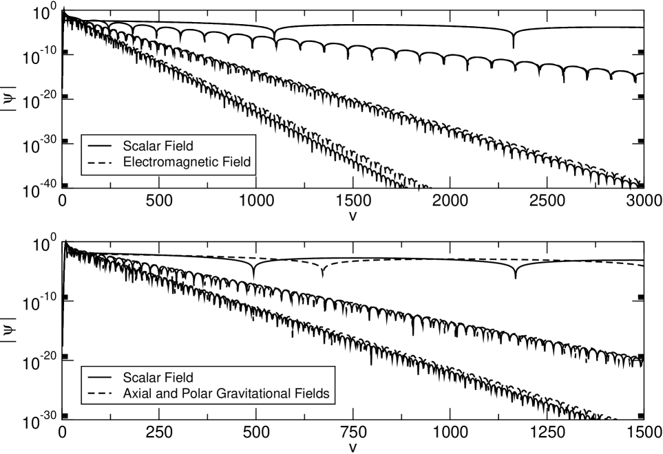
Figure 1: Decay of the scalar and electromagnetic fields with $\ell=1$, and of the scalar, axial, and polar gravitational fields, with $\ell=2$, with the SdS geometry approaching the near extreme limit.The parameters for the geometry are $m=1.0$ and $\bar{\delta}=0.01,0.1,0.3$.

Direct calculation of the wave functions confirms that, in the near extreme limit, their dynamics is simple, with the late-time decay of the fields being dominated by quasinormal modes. All the types of perturbation tend to coincide near the extreme limit. In addition, as we approach the extreme limit, the oscillation period increases and the exponential decay rate decreases. These conclusions, illustrated in Fig. 1 for $\ell=1,2$, are consistent with the ones presented in Cardoso-03 ; Molina-03 .

By using a nonlinear fitting based on a $\chi^{2}$ analysis, it is possible to estimate the real and imaginary parts of the $n=0$ quasinormal mode. These results can be compared with the analytical expressions in the near extreme cases. In Fig. 2, we analyze the dependence of the frequencies on $\ell$. The accordance between analytic and numerical data is extremely good.

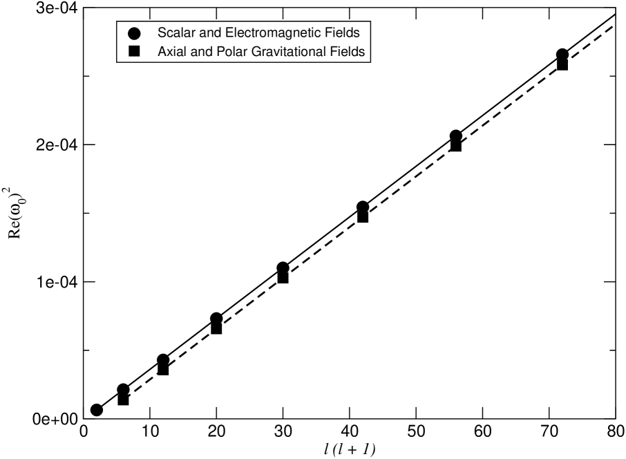
Figure 2: Curve of $\textrm{Re}(\omega_{0})^{2}$ with $\ell(\ell+1)$, for the scalar, electromagnetic and gravitational fields, in the near extreme limit. The dots are the numerical results and the solid lines represent the analytical results. The parameters for the geometry are $m=1.0$ and $\bar{\delta}=0.01$.

IV.2 Reissner–Nordström–de Sitter black hole

For the RNdS case, the near extreme limit corresponds to the situation where the event and cosmological horizons are very close to each other. It is natural to define the dimensionless parameter $\delta$ as

$$\delta=\frac{r_{c}-r_{+}}{r_{+}}\ ,$$ (43)

where $0<\delta\ll 1$. In this limit the dynamics can be analytically characterized, as has been analyzed in Cardoso-03 . More general settings, including RNdS geometries, were explored in Molina-03 .

The function $h(x)\equiv h(r(x))$ can be analytically calculated Cardoso-03 ; Molina-03 , with the result

$$h(x)=\frac{(r_{c}-r_{+})\kappa_{+}}{2\cosh^{2}(\kappa_{+}x)}+O\left(\delta^{3}\right)\ .$$ (44)

We have five different fields at hand: the scalar field ($Z_{sc}$), two axial fields ($Z_{1}^{-}$, $Z_{2}^{-}$), and two polar fields ($Z_{1}^{+}$, $Z_{2}^{+}$). For each one, we have a different potential. In the near extreme limit, we have

$$V(x)=\Omega(r_{+})h(x)+O\left(\delta\right)=\frac{V_{0}}{\cosh^{2}\left(\kappa_{+}x\right)}+O\left(\delta\right)\ .$$ (45)

The constant $V_{0}$ in the scalar case is denoted by $V_{0}^{sc}$, in the axial cases by $\{V_{0}^{1-},V_{0}^{2-}\}$, and in the polar cases by $\{V_{0}^{1+},V_{0}^{2+}\}$. The foregoing expression is a Pöschl-Teller potential Poschl-33 .

For the scalar field, $V_{0}^{sc}$ has been calculated in Molina-03 , and is given by

$$V_{0}^{sc}=\frac{\ell(\ell+1)(r_{c}-r_{+})\kappa_{+}}{2r_{+}^{2}}\ .$$ (46)

We proceed to the analysis of the coupled electromagnetic and gravitational fields. We take the analytical expressions for all potentials $V_{1,2}^{\pm}$ and we go to the near extreme limit. For the two axial potentials, we have

$$V_{0}^{1-}=\frac{(r_{c}-r_{+})\kappa_{+}}{2r_{+}^{4}}\left[\ell(\ell+1)r_{+}^{2}+4q^{2}-r_{+}S_{1}\right]\ ,$$ (47)

$$V_{0}^{2-}=\frac{(r_{c}-r_{+})\kappa_{+}}{2r_{+}^{4}}\left[\ell(\ell+1)r_{+}^{2}+4q^{2}-r_{+}S_{2}\right]\ ,$$ (48)

where

$$S_{1}=3m-\sqrt{9m^{2}+4(\ell+2)(\ell-1)q^{2}}\ ,$$ (49)

$$S_{2}=3m+\sqrt{9m^{2}+4(\ell+2)(\ell-1)q^{2}}\ .$$ (50)

We can now turn to the two polar potentials. The constants $V_{0}^{1+}$ and $V_{0}^{2+}$ are given by

$$V_{0}^{1+}=\frac{\kappa_{+}(r_{c}-r_{+})}{2r_{+}^{4}}\left[\frac{\left(2cr_{+}^{2}+3mr_{+}+r_{+}\sqrt{9m^{2}+8cq^{2}}\right)\left(cr_{+}+m+\frac{2\Lambda r_{+}^{3}}{3}\right)}{cr_{+}+3m-\frac{2q^{2}}{r_{+}}}+C\right]\ ,$$ (51)

$$V_{0}^{2+}=\frac{\kappa_{+}(r_{c}-r_{+})}{2r_{+}^{4}}\left[\frac{\left(2cr_{+}^{2}+3mr_{+}-r_{+}\sqrt{9m^{2}+8cq^{2}}\right)\left(cr_{+}+m+\frac{2\Lambda r_{+}^{3}}{3}\right)}{cr_{+}+3m-\frac{2q^{2}}{r_{+}}}+C\right]\ ,$$ (52)

with $C=2mr_{+}-2q^{2}-2\Lambda r_{+}^{4}/3$ and $2c=(\ell+2)(\ell-1)$. The quasinormal modes associated with the Pöschl-Teller potential have been extensively studied Ferrari-84 ; Beyer-99 . The frequencies $\omega_{n}$ are given by

$$\frac{\omega_{n}}{\kappa_{+}}=\sqrt{\frac{V_{0}}{\kappa_{+}^{2}}-\frac{1}{4}}-i\left(n+\frac{1}{2}\right)\ ,$$ (53)

with $n\in\{0,1,\ldots\}$ labeling the modes. Using expression (53) and the expression for $V_{0}$, the frequencies can be easily calculated.

We can also use the numerical method to analyze the field decay in the near extreme limit. Using a nonlinear fitting based on $\chi^{2}$ analysis for the wave functions, we can estimate the quasinormal frequencies. These results can be compared with the analytical expressions in the near extreme cases. The accordance between both sets of results is extremely good. We illustrate this point in Figs. 3–5.

Direct calculation of the wave functions confirms that, in the near extreme limit, the dynamics of the fields is simple, with the late-time decay being completely dominated by quasinormal modes.

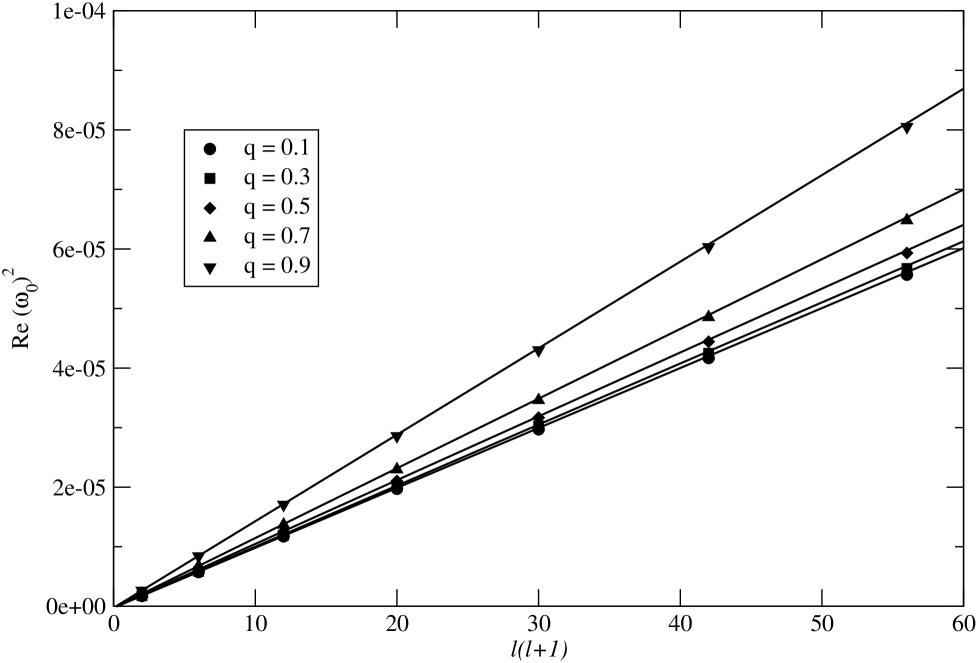
Figure 3: Near extreme fundamental frequencies for different values of the charge $q$, for the lower multipole mode of the scalar field. Analytical values are represented by straight lines, and numerical values appear as dots. The parameters for the geometry are $m=1.0$ and $\delta=10^{-3}$.

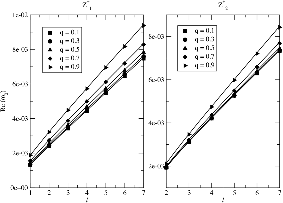
Figure 4: Near extreme fundamental frequencies for different values of the charge $q$, for the lower multipole mode of the polar fields. On the left are the data for $Z_{1}^{+}$ and, on the left, for $Z_{2}^{+}$. The parameters for the geometry are $m=1.0$ and $\delta=10^{-3}$.

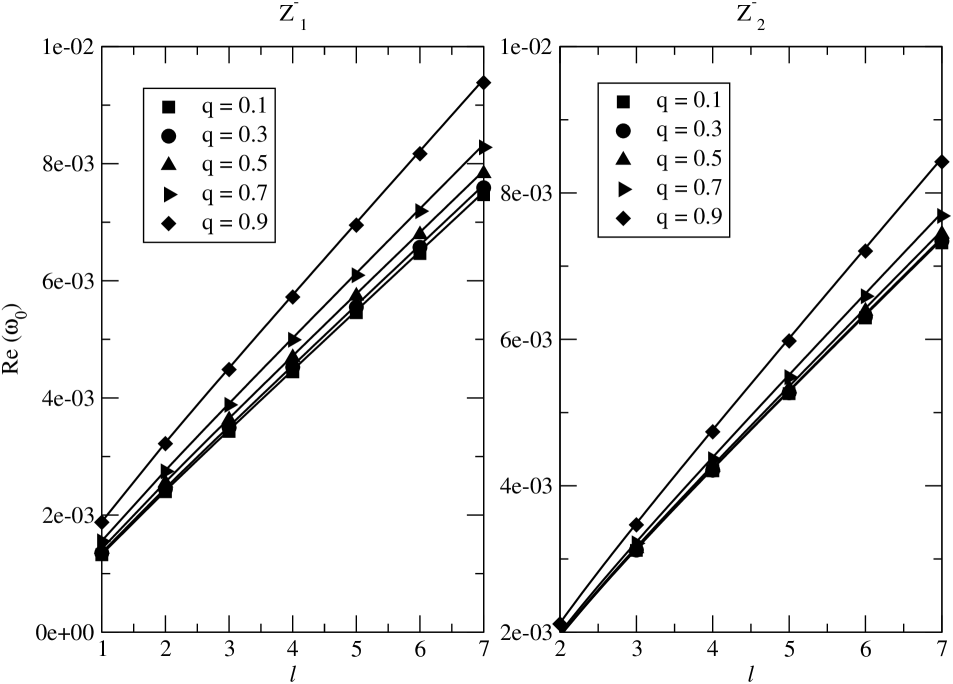
Figure 5: Near extreme fundamental frequencies for different values of the charge $q$, for the lower multipole mode of the axial fields. The data for $Z_{1}^{-}$ appear on the left, and those for $Z_{2}^{-}$, on the right. The parameters for the geometry are $m=1.0$ and $\delta=10^{-3}$.

V Intermediary Region in Parameter Space

V.1 Schwarzschild–de Sitter black hole

V.1.1 Scalar field with $\ell=0$

Only scalar perturbations can have zero total angular momentum. Solutions of Eq. (10) with $\ell=0$ lead to a constant tail, as already shown in Brady-97 ; Brady-99 . This is confirmed in Fig. 6. The novelty here is the dependence of the asymptotic value on the $\dot{\psi}_{\ell}(0,x)$ initial condition. Figure 6 reveals the appearance of the constant value $\phi_{0}$ for large $t$, and its dependence on $\dot{\psi}_{\ell}(0,x)$. Note that $\phi_{0}$ falls below $10^{-7}$ for $\dot{\psi}_{\ell}(0,x)=0$. These results are in accordance with the analytical predictions of Brady-99 , which give

$$\psi\left(\infty,r\right)=\frac{r}{r_{c}^{2}}\int_{0}^{r_{c}}\dot{\psi}(0,s)s\frac{ds}{h^{\prime}(s)}.$$ (54)

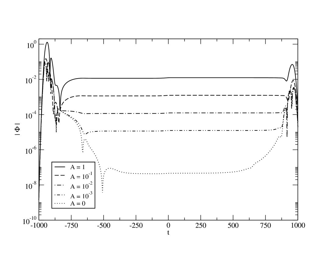
Figure 6: Asymptotic solutions $\phi(x,t)$ obtained by noncharacteristic numerical integration with $\ell=0$, $\Lambda=10^{-4}$ and $m=1.0$. The curves correspond to different values of $A$ in the initial condition (32).

V.1.2 Fields with $\ell>0$

We can have scalar and vector fields with angular momentum $\ell=1$, and with $\ell>1$, it is possible to introduce gravitational fields also. Their behavior is described in general by three phases. The first corresponds to the quasinormal modes generated from the presence of the black hole itself. A little later there is a region of power law decay, which continues indefinitely in an asymptotic flat space. In the presence of a positive cosmological constant, however, an exponential decay takes over in the latest period.

As the separation of the horizons increases, the quasinormal frequencies deviate from those predicted by expressions (41) and (LABEL:w-qext-gr). In Fig. 7, this is illustrated for $\ell=1,2$. Some qualitatively different effects show up when we turn away from the near extreme limit. For a small cosmological constant the asymptotic behavior is dominated by an exponentially decaying mode rather than by a quasinormal mode, for all perturbations considered.

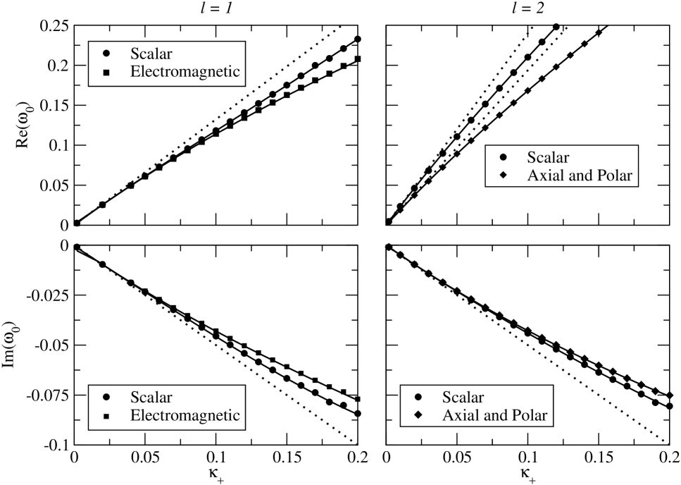
Figure 7: Graphs of the real and imaginary part of the fundamental frequencies $(n=0)$ with $\kappa_{+}$. The dotted lines are the near extreme results, the dots are the numerical results and the continuous curves are the semianalytic results. In the graphs, $m=1.0$.

It is interesting to compare the values obtained for the fundamental modes using the numerical and semianalytic methods. We find that the agreement between them is good, for the whole range of $\Lambda$. The difference is smaller for the first values of $\ell$. This is expected, since the numerical calculations work better in this region. In Table 1, we illustrate these observations with a few values of $\Lambda$. It is important to mention that quasinormal frequencies for the SdS black hole were already calculated in a recent paper Zhidenko , by applying a variation of the WKB method used here Konoplya-03 . There are earlier papers calculating quasinormal modes in this geometry, for example, dsqnm .

Table 1: Fundamental frequencies for the scalar field in SdS, obtained using the numerical and semianalytical methods. In this table, $m=1.0$.

q = 0		Numerical		Semianalytical
$\ell$	$\Lambda$	Re($\omega_{0}$)	-Im($\omega_{0}$)	Re($\omega_{0}$)	-Im($\omega_{0}$)
1	$10^{-5}$	2.930$\times 10^{-1}$	9.753$\times 10^{-1}$	2.911$\times 10^{-1}$	9.780$\times 10^{-2}$
	$10^{-4}$	2.928$\times 10^{-1}$	9.764$\times 10^{-2}$	2.910$\times 10^{-1}$	9.797$\times 10^{-2}$
	$10^{-3}$	2.914$\times 10^{-1}$	9.726$\times 10^{-2}$	2.896$\times 10^{-1}$	9.771$\times 10^{-2}$
	$10^{-2}$	2.770$\times 10^{-1}$	9.455$\times 10^{-2}$	2.753$\times 10^{-1}$	9.490$\times 10^{-2}$
	$10^{-1}$	8.159$\times 10^{-2}$	3.123$\times 10^{-2}$	8.144$\times 10^{-2}$	3.137$\times 10^{-2}$
2	$10^{-5}$	4.840$\times 10^{-1}$	9.653$\times 10^{-2}$	4.832$\times 10^{-1}$	9.680$\times 10^{-2}$
	$10^{-4}$	4.833$\times 10^{-1}$	8.948$\times 10^{-2}$	4.830$\times 10^{-1}$	9.677$\times 10^{-2}$
	$10^{-3}$	4.816$\times 10^{-1}$	8.998$\times 10^{-2}$	4.809$\times 10^{-1}$	9.643$\times 10^{-2}$
	$10^{-2}$	4.598$\times 10^{-1}$	8.880$\times 10^{-2}$	4.592$\times 10^{-1}$	9.290$\times 10^{-2}$
	$10^{-1}$	1.466$\times 10^{-1}$	3.068$\times 10^{-2}$	1.466$\times 10^{-1}$	3.070$\times 10^{-2}$
3	$10^{-5}$	6.769$\times 10^{-1}$	8.662$\times 10^{-2}$	6.752$\times 10^{-1}$	9.651$\times 10^{-2}$
	$10^{-4}$	6.754$\times 10^{-1}$	8.654$\times 10^{-2}$	6.749$\times 10^{-1}$	9.647$\times 10^{-2}$
	$10^{-3}$	6.732$\times 10^{-1}$	8.660$\times 10^{-2}$	6.720$\times 10^{-1}$	9.611$\times 10^{-2}$
	$10^{-2}$	6.437$\times 10^{-2}$	9.200$\times 10^{-2}$	6.428$\times 10^{-2}$	9.235$\times 10^{-2}$
	$10^{-1}$	2.091$\times 10^{-2}$	3.054$\times 10^{-2}$	2.091$\times 10^{-2}$	3.056$\times 10^{-2}$

Table 2: Fundamental frequencies for the electromagnetic field in SdS, obtained using the numerical and semianalytical methods. In this table, $m=1.0$.

q = 0		Numerical		Semianalytical
$\ell$	$\Lambda$	Re($\omega_{0}$)	-Im($\omega_{0}$)	Re($\omega_{0}$)	-Im($\omega_{0}$)
1	$10^{-5}$	2.481$\times 10^{-1}$	9.226$\times 10^{-2}$	2.459$\times 10^{-1}$	9.310$\times 10^{-2}$
	$10^{-4}$	2.481$\times 10^{-1}$	9.223$\times 10^{-2}$	2.457$\times 10^{-1}$	9.307$\times 10^{-2}$
	$10^{-3}$	2.475$\times 10^{-1}$	9.176$\times 10^{-2}$	2.448$\times 10^{-1}$	9.270$\times 10^{-2}$
	$10^{-2}$	2.374$\times 10^{-1}$	8.839$\times 10^{-2}$	2.352$\times 10^{-1}$	8.896$\times 10^{-2}$
	$10^{-1}$	8.035$\times 10^{-2}$	3.027$\times 10^{-2}$	8.023$\times 10^{-2}$	3.033$\times 10^{-2}$
2	$10^{-5}$	4.577$\times 10^{-1}$	8.985$\times 10^{-2}$	4.571$\times 10^{-1}$	9.506$\times 10^{-2}$
	$10^{-4}$	4.575$\times 10^{-1}$	8.991$\times 10^{-2}$	4.569$\times 10^{-1}$	9.502$\times 10^{-2}$
	$10^{-3}$	4.559$\times 10^{-1}$	9.439$\times 10^{-2}$	4.551$\times 10^{-1}$	9.464$\times 10^{-2}$
	$10^{-2}$	4.371$\times 10^{-1}$	8.941$\times 10^{-2}$	4.364$\times 10^{-1}$	9.074$\times 10^{-2}$
	$10^{-1}$	1.458$\times 10^{-1}$	3.037$\times 10^{-2}$	1.458$\times 10^{-1}$	3.038$\times 10^{-2}$
3	$10^{-5}$	6.578$\times 10^{-1}$	8.365$\times 10^{-2}$	6.567$\times 10^{-1}$	9.563$\times 10^{-2}$
	$10^{-4}$	6.576$\times 10^{-1}$	8.349$\times 10^{-2}$	6.564$\times 10^{-1}$	9.559$\times 10^{-2}$
	$10^{-3}$	6.547$\times 10^{-1}$	8.399$\times 10^{-2}$	6.538$\times 10^{-1}$	9.520$\times 10^{-2}$
	$10^{-2}$	6.276$\times 10^{-2}$	8.852$\times 10^{-2}$	6.267$\times 10^{-1}$	9.125$\times 10^{-2}$
	$10^{-1}$	2.085$\times 10^{-2}$	3.039$\times 10^{-3}$	2.085$\times 10^{-1}$	3.040$\times 10^{-2}$

Table 3: Fundamental frequencies for the axial and polar gravitational fields in SdS, obtained using the numerical and semianalytical methods. In this table, $m=1.0$.

q = 0		Numerical		Semianalytical
$\ell$	$\Lambda$	Re($\omega_{0}$)	-Im($\omega_{0}$)	Re($\omega_{0}$)	-Im($\omega_{0}$)
2	$10^{-5}$	3.738$\times 10^{-1}$	8.883$\times 10^{-2}$	3.731$\times 10^{-1}$	8.921$\times 10^{-2}$
	$10^{-4}$	3.737$\times 10^{-1}$	8.880$\times 10^{-2}$	3.730$\times 10^{-1}$	8.918$\times 10^{-2}$
	$10^{-3}$	3.721$\times 10^{-1}$	8.850$\times 10^{-2}$	3.715$\times 10^{-1}$	8.888$\times 10^{-2}$
	$10^{-2}$	3.566$\times 10^{-1}$	8.538$\times 10^{-2}$	3.560$\times 10^{-1}$	8.572$\times 10^{-2}$
	$10^{-1}$	1.179$\times 10^{-1}$	3.020$\times 10^{-2}$	1.179$\times 10^{-1}$	3.023$\times 10^{-2}$
3	$10^{-5}$	5.999$\times 10^{-1}$	8.677$\times 10^{-2}$	5.992$\times 10^{-1}$	9.272$\times 10^{-2}$
	$10^{-4}$	5.996$\times 10^{-1}$	8.676$\times 10^{-2}$	5.990$\times 10^{-1}$	9.269$\times 10^{-2}$
	$10^{-3}$	5.972$\times 10^{-1}$	8.971$\times 10^{-2}$	5.966$\times 10^{-1}$	9.234$\times 10^{-2}$
	$10^{-2}$	5.725$\times 10^{-1}$	8.695$\times 10^{-2}$	5.718$\times 10^{-1}$	8.874$\times 10^{-2}$
	$10^{-1}$	1.900$\times 10^{-1}$	3.030$\times 10^{-2}$	1.900$\times 10^{-2}$	3.032$\times 10^{-2}$
4	$10^{-5}$	8.106$\times 10^{-1}$	8.810$\times 10^{-2}$	8.091$\times 10^{-1}$	9.417$\times 10^{-2}$
	$10^{-4}$	8.102$\times 10^{-1}$	8.781$\times 10^{-2}$	8.087$\times 10^{-1}$	9.413$\times 10^{-2}$
	$10^{-3}$	8.070$\times 10^{-1}$	8.799$\times 10^{-2}$	8.055$\times 10^{-1}$	9.376$\times 10^{-2}$
	$10^{-2}$	7.733$\times 10^{-2}$	8.714$\times 10^{-2}$	7.720$\times 10^{-1}$	9.000$\times 10^{-2}$
	$10^{-1}$	2.564$\times 10^{-2}$	3.034$\times 10^{-3}$	2.563$\times 10^{-1}$	3.036$\times 10^{-2}$

The first higher $n$ modes cannot be obtained from the numerical solution, but can be calculated by the semianalytical method. As the cosmological constant decreases, the real and imaginary parts of the frequencies increase, up to the limit where the geometry is asymptotically flat. The behavior of the modes is illustrated in Fig. 8. The behavior of the electromagnetic field is similar.

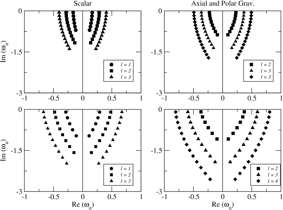
Figure 8: Quasinormal modes of the scalar, axial and polar gravitational fields, for higher modes. The parameter for the curves are $m=1.0$ and $\Lambda=10^{-3}$.

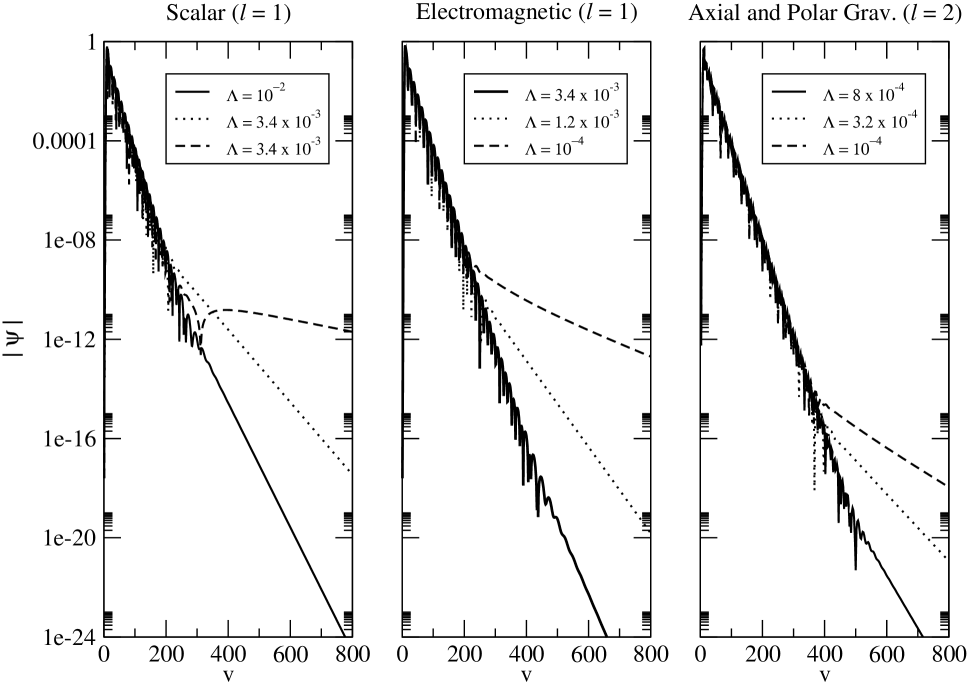
Figure 9: Exponential tail for the scalar and electromagnetic fields with $\ell=1$, and for the axial and polar gravitational field with $\ell=2$. In the graphs, $m=1.0$.

A $\chi^{2}$ analysis of the data presented in Figure 9 shows that the massless scalar, electromagnetic, and gravitational perturbations in SdS geometry behave as

$$\psi_{\ell}^{sc}\sim e^{-k_{exp}^{sc}t} {\rm with} t\rightarrow\infty\ ,$$ (55)

$$\psi_{\ell}^{el}\sim e^{-k_{exp}^{el}t} {\rm with} t\rightarrow\infty\ ,$$ (56)

$$\psi_{\ell}^{ax}\sim e^{-k_{exp}^{ax}t} {\rm with} t\rightarrow\infty\ ,$$ (57)

$$\psi_{\ell}^{po}\sim e^{-k_{exp}^{po}t} {\rm with} t\rightarrow\infty$$ (58)

for $t$ sufficiently large. At the event and the cosmological horizons, $t$ is substituted, respectively, by $v$ and $u$.

The numerical simulations developed in the present work reveal an interesting transition between oscillatory modes and exponentially decaying modes. As shown in Fig. 10, as the cosmological constant increases, the absolute value of $-\textrm{Im}(\omega_{0})$ decreases.

Above a certain critical value of $\Lambda$ we do not observe the exponential tail, since the coefficient $k_{exp}$ is larger than $-\textrm{Im}(\omega_{0})$ and thus the decaying quasinormal mode dominates. But for $\Lambda$ smaller than this critical value, $-\textrm{Im}(\omega_{0})$ turns out to be larger than $k_{exp}$, and the exponential tail dominates. Certainly, for a small enough cosmological constant, the exponential tail dominates in the various cases considered here.

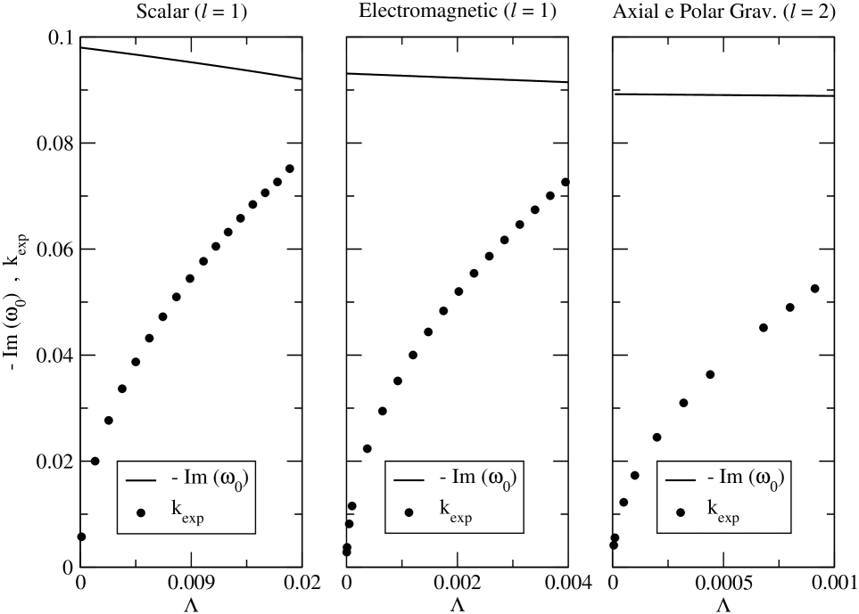
Figure 10: Approaching of $-\textrm{Im}(\omega_{0})$ and $k_{exp}$, for the scalar, electromagnetic and gravitational fields, in the SdS geometry. Above a certain critical value of $\Lambda$ (roughly $1.7\times 10^{-2}$, $4.0\times 10^{-3}$ and $1.2\times 10^{-3}$ respectively, for the parameters used in the graphs), a tail it is not observed. For all curves, the mass is set to $m=1.0$.

Another aspect worth mentioning in the intermediate region is the dependence of the parameters $k_{exp}^{sc}$, $k_{exp}^{el}$, $k_{exp}^{ax}$, and $k_{exp}^{po}$ on $\ell$ and $\kappa_{c}$. The results suggest that the $k_{exp}$ are at least second differentiable functions of $\kappa_{c}$. Therefore, close to $\kappa_{c}=0$, we approximate

$$k_{exp}^{sc}(\kappa_{c})\approx\ell\left(\kappa_{c}+c^{sc}\kappa_{c}^{2}\right)\ ,$$ (59)

$$k_{exp}^{el}(\kappa_{c})\approx k_{exp}^{ax}(\kappa_{c})\approx k_{exp}^{po}(\kappa_{c})\approx(\ell+1)\left(\kappa_{c}+c^{e-g}\kappa_{c}^{2}\right)\ .$$ (60)

Previous results are illustrated in Fig. 11.

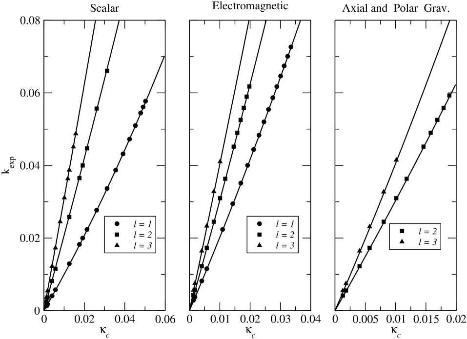
Figure 11: Dependence of $k_{exp}$ with $\kappa_{c}$ and $\ell$, in the SdS geometry. The symbols indicate the numerical values, and the solid lines are the appropriate fittings. For the left graph: $k_{exp}^{sc}=1.077\times 10^{-4}+0.984\kappa_{c}+3.545\kappa_{c}^{2}$, $k_{exp}^{sc}=-1.863\times 10^{-4}+2.010\kappa_{c}+2.608\kappa_{c}^{2}$ and $k_{exp}^{sc}=-1.959\times 10^{-4}+3.028\kappa_{c}+2.978\kappa_{c}^{2}$. For the center graph: $k_{exp}^{el}=2.082\times 10^{-4}+1.988\kappa_{c}+6.141\kappa_{c}^{2}$, $k_{exp}^{el}=2.712\times 10^{-4}+2.974\kappa_{c}+8.284\kappa_{c}^{2}$ and $k_{exp}^{el}=3.737\times 10^{-4}+3.984\kappa_{c}+4.517\kappa_{c}^{2}$. For the right graph: $k_{exp}^{ax}=2.616\times 10^{-4}+2.974\kappa_{c}+9.895\kappa_{c}^{2}$ and $k_{exp}^{ax}=4.484\times 10^{-4}+3.896\kappa_{c}+18.92\kappa_{c}^{2}$. In the graphs, $m=1.0$.

V.2 Reissner–Nordström–de Sitter black hole

We assess here the behavior of the fields in RNdS exterior geometries that are not near extreme, nor close to the asymptotically flat limit. Direct numerical simulations and semianalytical (WKB) methods were largely employed to characterize the fields in this region.

For scalar perturbations with $\ell=0$, the effective potential is not positive definite. As already shown in Brady-97 ; Brady-99 , solutions of Eq. (10) with $\ell=0$ lead to a constant tail. It was observed that in the SdS geometry there is a dependence of the asymptotic value on the $\dot{\psi}_{\ell}(0,x)$ initial condition, in the context of a Cauchy type initial value problem. We have checked that the introduction of electric charge does not alter this picture.

If $\ell>0$, we introduce the $Z_{1}^{\pm}$ fields, and for $\ell>1$ the $Z_{2}^{\pm}$ fields can also be analyzed. The first point studied is the quasinormal phase. If the cosmological constant is high enough, the decay is dominated by quasinormal modes, even when they no longer are accurately predicted by the expressions (53). This scenario, illustrated in Fig. 12, is valid for all fields considered, with any charge smaller than its critical value.

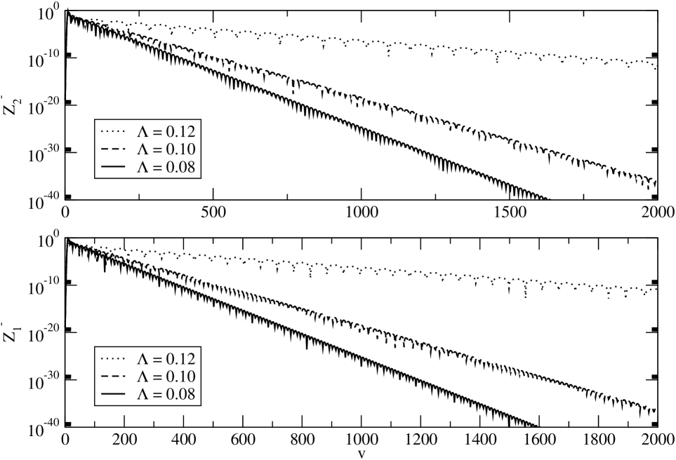
Figure 12: Quasinormal modes for RNdS $Z_{1}^{-}$ and $Z_{2}^{-}$ fields. The parameters for the geometry are $q=0.5$ and $m=1.0$. We have used $\ell=2$. The results are similar for the other fields considered.

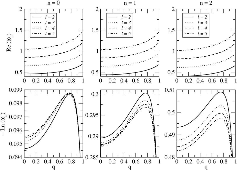
Figure 13: Dependence of $Z_{1}^{+}$ field frequencies on $q$, for both the real and imaginary parts, in RNdS. The results are qualitatively similar for the other fields considered. The parameters are $m=1.0$ and $\Lambda=10^{-4}$.

We have observed that the influence of the electric charge is mild, although not trivial. The range of variation of the quasinormal modes with the charge is not very large. We illustrate this point in Fig. 13. It is interesting to compare the values obtained for the fundamental modes using the numerical and semianalytical methods. We find a very good agreement between these results. The difference is smaller for the first values of $\ell$. This is expected, since the numerical calculations work better in this region. In Tables 4-7, we illustrate these observations for a few values of $\Lambda$ and $q$.

Table 4: Fundamental frequencies for the $Z_{1}^{-}$ field in RNdS, with $q=0.5$ and $m=1.0$, using the numerical and semianalytical methods.

q = 0.5		Numerical		Semianalytical
$\ell$	$\Lambda$	Re($\omega_{0}$)	-Im($\omega_{0}$)	Re($\omega_{0}$)	-Im($\omega_{0}$)
1	$10^{-5}$	2.71$\times 10^{-1}$	9.51$\times 10^{-2}$	3.28$\times 10^{-1}$	9.53$\times 10^{-2}$
	$10^{-4}$	2.71$\times 10^{-1}$	9.50$\times 10^{-2}$	3.28$\times 10^{-1}$	9.53$\times 10^{-2}$
	$10^{-3}$	2.70$\times 10^{-1}$	9.47$\times 10^{-2}$	3.27$\times 10^{-1}$	9.49$\times 10^{-2}$
	$10^{-2}$	2.60$\times 10^{-1}$	9.11$\times 10^{-2}$	3.15$\times 10^{-1}$	9.14$\times 10^{-2}$
	$10^{-1}$	1.16$\times 10^{-1}$	4.08$\times 10^{-2}$	1.40$\times 10^{-1}$	4.08$\times 10^{-2}$
2	$10^{-5}$	4.94$\times 10^{-1}$	9.72$\times 10^{-2}$	4.94$\times 10^{-1}$	9.71$\times 10^{-2}$
	$10^{-4}$	4.93$\times 10^{-1}$	9.72$\times 10^{-2}$	4.94$\times 10^{-1}$	9.71$\times 10^{-2}$
	$10^{-3}$	4.91$\times 10^{-1}$	9.68$\times 10^{-2}$	4.92$\times 10^{-1}$	9.67$\times 10^{-2}$
	$10^{-2}$	4.73$\times 10^{-1}$	9.31$\times 10^{-2}$	4.73$\times 10^{-1}$	9.30$\times 10^{-2}$
	$10^{-1}$	2.09$\times 10^{-1}$	4.10$\times 10^{-2}$	2.09$\times 10^{-1}$	4.16$\times 10^{-2}$
3	$10^{-5}$	7.05$\times 10^{-1}$	8.95$\times 10^{-2}$	7.05$\times 10^{-1}$	9.77$\times 10^{-2}$
	$10^{-4}$	7.05$\times 10^{-1}$	8.94$\times 10^{-2}$	7.05$\times 10^{-1}$	9.76$\times 10^{-2}$
	$10^{-3}$	7.02$\times 10^{-1}$	8.87$\times 10^{-2}$	7.02$\times 10^{-1}$	9.73$\times 10^{-2}$
	$10^{-2}$	6.77$\times 10^{-1}$	8.50$\times 10^{-2}$	6.76$\times 10^{-1}$	9.35$\times 10^{-2}$
	$10^{-1}$	2.98$\times 10^{-1}$	4.10$\times 10^{-2}$	2.98$\times 10^{-1}$	4.10$\times 10^{-2}$

Table 5: Fundamental frequencies for the $Z_{2}^{-}$ field in RNdS, with $q=0.5$ and $m=1.0$, using the numerical and semianalytical methods.

q = 0.5		Numerical		Semianalytical
$\ell$	$\Lambda$	Re($\omega_{0}$)	-Im($\omega_{0}$)	Re($\omega_{0}$)	-Im($\omega_{0}$)
2	$10^{-5}$	3.82$\times 10^{-1}$	8.96$\times 10^{-2}$	3.81$\times 10^{-1}$	8.98$\times 10^{-2}$
	$10^{-4}$	3.82$\times 10^{-1}$	8.96$\times 10^{-2}$	3.81$\times 10^{-1}$	8.98$\times 10^{-2}$
	$10^{-3}$	3.80$\times 10^{-1}$	8.93$\times 10^{-2}$	3.80$\times 10^{-1}$	8.95$\times 10^{-2}$
	$10^{-2}$	3.66$\times 10^{-1}$	8.67$\times 10^{-2}$	3.65$\times 10^{-1}$	8.67$\times 10^{-2}$
	$10^{-1}$	1.60$\times 10^{-1}$	4.06$\times 10^{-2}$	1.60$\times 10^{-1}$	4.05$\times 10^{-2}$
3	$10^{-5}$	6.13$\times 10^{-1}$	8.59$\times 10^{-2}$	6.12$\times 10^{-1}$	9.33$\times 10^{-2}$
	$10^{-4}$	6.13$\times 10^{-1}$	8.59$\times 10^{-2}$	6.12$\times 10^{-1}$	9.32$\times 10^{-2}$
	$10^{-3}$	6.10$\times 10^{-1}$	8.59$\times 10^{-2}$	6.10$\times 10^{-1}$	9.29$\times 10^{-2}$
	$10^{-2}$	5.88$\times 10^{-1}$	8.50$\times 10^{-2}$	5.87$\times 10^{-1}$	8.97$\times 10^{-2}$
	$10^{-1}$	2.58$\times 10^{-1}$	4.07$\times 10^{-2}$	2.59$\times 10^{-1}$	4.07$\times 10^{-2}$

Table 6: Fundamental frequencies for the $Z_{1}^{+}$ field in RNdS, with $q=0.5$ and $m=1.0$, using the numerical and semianalytical methods.

q = 0.5		Numerical		Semianalytical
$\ell$	$\Lambda$	Re($\omega_{0}$)	-Im($\omega_{0}$)	Re($\omega_{0}$)	-Im($\omega_{0}$)
1	$10^{-5}$	2.71$\times 10^{-1}$	9.51$\times 10^{-2}$	2.69$\times 10^{-1}$	9.55$\times 10^{-2}$
	$10^{-4}$	2.71$\times 10^{-1}$	9.50$\times 10^{-2}$	2.68$\times 10^{-1}$	9.55$\times 10^{-2}$
	$10^{-3}$	2.70$\times 10^{-1}$	9.47$\times 10^{-2}$	2.67$\times 10^{-1}$	9.51$\times 10^{-1}$
	$10^{-2}$	2.60$\times 10^{-1}$	9.11$\times 10^{-2}$	2.57$\times 10^{-1}$	9.15$\times 10^{-2}$
	$10^{-1}$	1.16$\times 10^{-1}$	4.08$\times 10^{-2}$	1.16$\times 10^{-1}$	4.08$\times 10^{-2}$
2	$10^{-5}$	4.94$\times 10^{-1}$	9.71$\times 10^{-2}$	4.93$\times 10^{-1}$	9.72$\times 10^{-2}$
	$10^{-4}$	4.94$\times 10^{-1}$	9.71$\times 10^{-2}$	4.93$\times 10^{-1}$	9.72$\times 10^{-2}$
	$10^{-3}$	4.92$\times 10^{-1}$	9.67$\times 10^{-2}$	4.91$\times 10^{-1}$	9.68$\times 10^{-2}$
	$10^{-2}$	4.73$\times 10^{-1}$	9.30$\times 10^{-2}$	4.73$\times 10^{-1}$	9.31$\times 10^{-2}$
	$10^{-1}$	2.09$\times 10^{-1}$	4.16$\times 10^{-2}$	2.09$\times 10^{-1}$	4.10$\times 10^{-2}$
3	$10^{-5}$	7.05$\times 10^{-1}$	8.95$\times 10^{-2}$	7.05$\times 10^{-1}$	9.77$\times 10^{-2}$
	$10^{-4}$	7.05$\times 10^{-1}$	8.94$\times 10^{-2}$	7.05$\times 10^{-1}$	9.76$\times 10^{-2}$
	$10^{-3}$	7.02$\times 10^{-1}$	8.86$\times 10^{-2}$	7.02$\times 10^{-1}$	9.73$\times 10^{-2}$
	$10^{-2}$	6.77$\times 10^{-1}$	8.50$\times 10^{-2}$	6.76$\times 10^{-1}$	9.35$\times 10^{-2}$
	$10^{-1}$	2.98$\times 10^{-1}$	4.10$\times 10^{-2}$	2.98$\times 10^{-1}$	4.10$\times 10^{-2}$

Table 7: Fundamental frequencies for the $Z_{2}^{+}$ field in RNdS, with $q=0.5$ and $m=1.0$, using the numerical and semianalytical methods.

q = 0.5		Numerical		Semianalytical
$\ell$	$\Lambda$	Re($\omega_{0}$)	-Im($\omega_{0}$)	Re($\omega_{0}$)	-Im($\omega_{0}$)
2	$10^{-5}$	3.82$\times 10^{-1}$	8.96$\times 10^{-2}$	3.81$\times 10^{-1}$	8.99$\times 10^{-2}$
	$10^{-4}$	3.82$\times 10^{-1}$	8.95$\times 10^{-2}$	3.81$\times 10^{-1}$	8.97$\times 10^{-2}$
	$10^{-3}$	3.80$\times 10^{-1}$	8.93$\times 10^{-2}$	3.79$\times 10^{-1}$	8.94$\times 10^{-2}$
	$10^{-2}$	3.66$\times 10^{-1}$	8.64$\times 10^{-2}$	3.65$\times 10^{-1}$	8.66$\times 10^{-2}$
	$10^{-1}$	1.60$\times 10^{-1}$	4.13$\times 10^{-2}$	1.60$\times 10^{-1}$	4.05$\times 10^{-2}$
3	$10^{-5}$	6.13$\times 10^{-1}$	8.56$\times 10^{-2}$	6.12$\times 10^{-1}$	9.33$\times 10^{-2}$
	$10^{-4}$	6.13$\times 10^{-1}$	8.56$\times 10^{-2}$	6.12$\times 10^{-1}$	9.32$\times 10^{-2}$
	$10^{-3}$	6.10$\times 10^{-1}$	8.56$\times 10^{-2}$	6.10$\times 10^{-1}$	9.29$\times 10^{-2}$
	$10^{-2}$	5.88$\times 10^{-1}$	8.49$\times 10^{-2}$	5.87$\times 10^{-1}$	8.97$\times 10^{-2}$
	$10^{-1}$	2.58$\times 10^{-1}$	4.07$\times 10^{-2}$	2.58$\times 10^{-1}$	4.07$\times 10^{-2}$

For all fields considered, with a small enough cosmological constant, there is a qualitative change in the behavior of all fields considered. The late-time decay is dominated by an exponential tail. Therefore in the RNdS geometry we have

$$\psi_{\ell}^{sc}\sim e^{-k_{exp}^{sc}t} \mathrm{with} t\rightarrow\infty\ ,$$ (61)

$$Z_{1}^{\pm}\sim e^{-k_{exp}^{1\pm}t} \mathrm{with} t\rightarrow\infty\ ,$$ (62)

$$Z_{2}^{\pm}\sim e^{-k_{exp}^{2\pm}t} \mathrm{with} t\rightarrow\infty\ ,$$ (63)

for $t$ sufficiently large. At the event and the cosmological horizons $t$ is substituted by $v$ and $u$, respectively. Figure 14 illustrates this point, which was noted in Brady-97 ; Brady-99 for scalar fields, and we have extended this consideration to coupled electromagnetic and gravitational fields. In the aforementioned figure we compare the exponential tails at the event horizon for exterior RNdS geometries.

An important point is that, unlike the quasinormal mode frequencies, the exponential coefficients have shown no dependence on the black hole’s electric charge, for all kinds of fields at hand. Close to $\kappa_{c}=0$, our results are compatible with the expressions

$$k_{exp}^{sc}(\kappa_{c})\approx\ell\left(\kappa_{c}+c^{sc}\kappa_{c}^{2}\right)\ ,$$ (64)

$$k_{exp}^{i\,\pm}(\kappa_{c})\approx(\ell+1)\left(\kappa_{c}+c^{i\,\pm}\kappa_{c}^{2}\right)\ \ \,i=1,2\ ,$$ (65)

for any $q$ lower than its extreme value. The dynamics of the fields in de Sitter spacetimes is therefore very different from similar cases in anti–de Sitter geometries, in which for high charge there is an abrupt change in the fields’ decay Wang-01 . We have also explicitly assessed the behavior of the $Z_{1,2}^{\pm}$ fields as $q\rightarrow 0$, comparing their quasinormal frequencies and exponential tails to those observed in the SdS $Z^{\pm}$ fields. As anticipated, we found that the $Z_{2}^{+}$ field behaves like the SdS $Z^{+}$ field and that the $Z_{2}^{-}$ field behaves like the SdS $Z^{-}$ field, if the charge is small enough. We have observed that the RNdS fields $Z_{2}^{\pm}$ tend smoothly to the SdS fields $Z^{\pm}$.

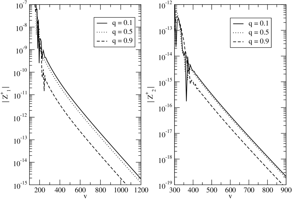
Figure 14: Tails of the $Z_{1}^{+}$ ($\ell=1$) and $Z_{2}^{+}$ ($\ell=2$) fields in RNdS. The parameters for the geometry are $\Lambda=10^{-4}$ and $m=1.0$. The results are similar for the other fields considered.

VI Approaching the Asymptotically Flat Geometry

Scalar fields in the SdS geometry near the asymptotically flat limit were studied in Brady-97 ; Brady-99 . In this case there is a clear separation between the event and the cosmological horizons, such that

$$\delta=\frac{r_{c}-r_{+}}{r_{+}}\gtrsim 50\ .$$ (66)

A new qualitative change occurs in this regime, namely, a decaying phase with a power law behavior. Such a phase occurs between the quasinormal mode decay and the exponential decay phases. The field cannot be simply described by a superposition of the various modes, which would imply a domination of the power law phase. This is illustrated in Fig. 15.

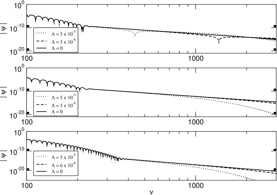
Figure 15: Approaching the asymptotically flat geometry in SdS. Straight lines in the log-log graphs indicate power law decay. In the graphs, $m=1.0$.

The situation for RNdS cases obeying Eq. (66) is presented in Fig. 16. As can be seen in this figure, we have a perfect power law tail developing for large $v$ when $\Lambda=0$, as expected. For the RNdS exterior geometry with low $\Lambda$ values, this power law tail appears quite clearly between the quasinormal zone and the exponential tail.

With such data, we can speak of three different regimes in the field dynamics when one approaches the asymptotically flat limit: first, a quasinormal regime, with its characteristic damped oscillations, followed by an intermediate regime for which the power law tail is visible, and a late-time region for which an exponential tail dominates. This qualitative picture is valid for all fields considered.

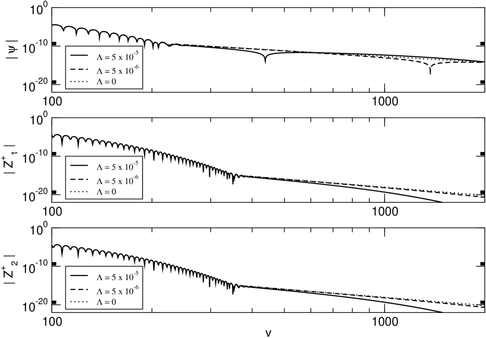
Figure 16: Scalar ($\ell=1$), $Z_{1}^{+}$ and $Z_{2}^{+}$ fields ($\ell=2$), approaching the asymptotically flat limit in RNdS. The parameters for the geometry are $q=0.5$ and $m=1.0$. The results are similar for the other fields considered.

VII Conclusions

We have identified three regimes, according to the value of $\Lambda$ for the decay of the scalar, electromagnetic, and gravitational (or $Z^{\pm}_{1,2}$ in RNdS) perturbations. Near the extreme limit (high $\Lambda$), we have analytic expressions for the effective potentials and the quasinormal frequencies. The decay is entirely dominated by the quasinormal modes (as in Beyer-99 ), that is, oscillatory decay characterized by a nonvanishing real part of the quasinormal frequency.

In an intermediary parameter region (lower $\Lambda$), the wave functions have an important qualitative change, with the appearance of an exponential tail. This tail dominates the decay for large time. Near the asymptotically flat limit ($\Lambda\ll 1$), we see an intermediary phase between the quasinormal modes and the exponential tail—a region of power law decay. When $\Lambda=0$, this region entirely dominates the late-time behavior.

Finally, for scalar fields with $\ell=0$ a constant decay mode appears, and its value depends on the $\dot{\psi}_{\ell}(0,x)$ initial condition. Fig. 6 reveals the appearance of the constant value $\phi_{0}$ for large $t$, and its dependence on $\dot{\psi}_{\ell}(0,x)$. The value of $\phi_{0}$ falls below $10^{-7}$ for $\dot{\psi}_{\ell}(0,x)=0$. These results are compatible with the analytical predictions of Brady-99 . The analytical characterization of these regions and the corresponding critical values of $\Lambda$ are crucial to a better understanding of these qualitatively different regimes.

A very important aspect of the field dynamics in the RNdS geometries is that the influence of the electric charge on the field behavior, in general, was shown to be quite restricted. In particular, we observed no dependence of the exponential tail coefficients with $q$. This contrasts with previous results obtained in the anti–de Sitter case Wang-01 , where the charge plays a fundamental role in the tails. A deep understanding of this fact depends on new analytical asymptotic results along the lines of the ones obtained in Brady-99 . These points are now under investigation. Also, since the presence of a charge implies an internal structure similar to that of a rotating black hole, our results might be interpreted as a broader universality of the frequencies here obtained. This question deserves further study.

- (1) T. Regge and J. A. Wheeler, Phys. Rev. 108, 1063 (1957).
- (2) S. Chandrasekhar, The Mathematical Theory of Black Holes (Oxford University Press, Oxforf, 1983).
- (3) K. D. Kokkotas and B. G. Schmidt, Living Rev. Relativity 2, 2 (1999).
- (4) A. Riess et al. Astrophy. J. 116, 1009 (1998); S. Perlmutter et al., ibid. 517, 565 (1999).
- (5) V. Cardoso and J. P. S. Lemos, Phys. Rev. D 64, 084017 (2001).
- (6) B. Wang, C. Lin and E. Abdalla, Phys. Lett. B, 481, 79 (2000); R. A. Konoplya, Phys. Rev. D 66, 044009 (2002); E. Berti and K. D. Kokkotas, ibid. 67, 064020 (2003); V. Cardoso, R. Konoplya and J. P. S. Lemos, ibid. 68, 044024 (2003).
- (7) V. Cardoso and J. P. S. Lemos, Class. Quantum Grav. 18, 5257 (2001); V. Cardoso and J. P. S. Lemos, Phys. Rev. D 63, 124015 (2001); J. M. Zhu, B. Wang and E. Abdalla, ibid. 63, 124004 (2001); B. Wang, E. Abdalla and R. B. Mann, ibid. 65, 084006. (2002).
- (8) B. Wang, C. Molina and E. Abdalla, Phys. Rev. D 63, 084001 (2001).
- (9) H. Nariai, Sci. Rep. Tohoku Univ. 34, 160 (1950); 35, 62 (1951).
- (10) E. W. Leaver, Phys. Rev. D 34, 384 (1986).
- (11) E. S. C. Ching, P. T. Leung, W. M. Suen and K. Young, Phys. Rev. D 52, 2118 (1995).
- (12) G. Gamow, Zeits. F. Phys. 51 204 (1928).
- (13) P. R. Brady, C. M. Chambers, W. Krivan and P. Laguna, Phys. Rev. D 55, 7538 (1997).
- (14) P. R. Brady, C. M. Chambers, W. G. Laarakkers and E. Poisson, Phys. Rev. D 60, 064003 (1999).
- (15) B. F. Schutz and C. M. Will, Astrophys. J. 291, L33 (1985).
- (16) S. Iyer and C. M. Will, Phys. Rev. D 35, 3621 (1987).
- (17) S. Iyer, Phys. Rev. D 35, 3632 (1987); K. D. Kokkotas and B. F. Schutz, Phys. Rev. D 37, 3378 (1988).
- (18) R. A. Konoplya, Phys. Rev. D 68, 024018 (2003).
- (19) A. Zhidenko, Class. Quantum Grav. 21, 273 (2004).
- (20) S. Yoshida and T. Futamase, Numerical analysis of quasinormal modes in nearly extremal Schwarzschild–de Sitter spacetimes, gr-qc/0308077.
- (21) E. Abdalla, B. Wang, A. Lima-Santos and W.G. Qiu, Phys. Lett. B 538, 435 (2002); E. Abdalla, K.H.C. Castello-Branco, A. Lima-Santos, Mod. Phys. Lett. A 18, 1435 (2003).
- (22) R. Ruffini, J. Tiomno and C. Vishveshwara, Lettere al Nuovo Cimento 3, 211 (1972).
- (23) F. Mellor and I. Moss, Phys. Rev. D 41, 403 (1990).
- (24) C. Gundlach, R. Price and J. Pullin, Phys. Rev. D 49, 883 (1994).
- (25) R. Price, Phys. Rev. D 5, 2419 (1972).
- (26) A.R. Levander, Geophysics 53, 1425 (1988).
- (27) V. Cardoso and J. P. S. Lemos, Phys. Rev. D 67, 084020 (2003).
- (28) C. Molina, Phys. Rev. D 68, 064007 (2003).
- (29) G. Pöschl and E. Teller, Z. Phys. 83, 143 (1933).
- (30) V. Ferrari and B. Mashhoon, Phys. Rev. D 30, 295 (1984).
- (31) H. Beyer, Commun. Math. Phys. 204, 397 (1999).
- (32) H. Otsuki and T. Futamase, Prog. Theor. Phys. 85, 771 (1991); I. Moss and J. Norman, Class. Quantum Grav. 19, 2323 (2002).