Field propagation in the Schwarzschild-de Sitter black hole

Abstract

We present an exhaustive analysis of scalar, electromagnetic and gravitational perturbations in the background of a Schwarzchild-de Sitter spacetime. The field propagation is considered by means of a semi-analytical (WKB) approach and two numerical schemes: the characteristic and general initial value integrations. The results are compared near the extreme regime, and a unifying picture is established for the dynamics of different spin fields. Although some of the results just confirm usual expectations, a few surprises turn out to appear, as the dependence on the non-characteristic initial conditions of the non-vanishing asymptotic value for $\ell=0$ mode scalar fields.

I Introduction

Wave propagation around non trivial solutions of Einstein equations, black hole in particular, is an active field of research (see Regge-57 ; Chandrasekhar ; Kokkotas-99 and references therein). The perspective of gravitational waves detection in a near future and the great development of numerical general relativity have increased even more the activity on this field. Gravitational waves should be especially strong when emitted by black holes. The study of the propagation of perturbations around them is, hence, essential to provide templates for the gravitational waves identification. In the other hand, recent astrophysical observations indicate that the universe is undergoing an accelerated expansion phase, suggesting the existence of a small positive cosmological constant and that de Sitter (dS) geometry provides a good description of very large scales of the universe accel-exp . We notice also that string theory has recently motivated many works on asymptotically anti-de Sitter spacetimes (see, for instance, Cardoso-01 ; AdS-4d ; AdS-other ; Wang-01 ).

In this work, we perform an exhaustive investigation of scalar, electromagnetic and gravitational perturbations in the background of a Schwarzchild-de Sitter spacetime. We scan the full range of the cosmological constant, from the asymptotic flat case ($\Lambda=0$) up to the critical value of $\Lambda$ which characterizes the Nariai solution Nariai . Two different numerical methods and a higher order WKB analysis are used.

We remind that for any perturbation in the spacetimes we consider, after the initial transient phase there are two main contributions to the resulting asymptotic wave Leaver-86 ; Ching-95 : initially the so called quasinormal modes, which are suppressed at later time by the tails. The first can be understood as candidates to normal modes which, however, decay (their energy eigenvalues becomes complex), as in the ingenious mechanism first described by G. Gamow in the context of nuclear physics Gamow-28 . After the initial transient phase, the properties of resulting wave are more related to background spacetime rather than to the source itself.

It is well known that for asymptotic flat backgrounds the tails decay according to a power-law, whereas in a space with a positive cosmological constant the decay is exponential. Curiously, $\ell=0$ modes for scalar fields in dS spacetimes, contrasting to the asymptotic flat cases, approach exponentially a non vanishing asymptotic value Brady-97 ; Brady-99 . We detected, by using a non-characteristic numerical integration scheme, a dependence of this asymptotic value on the initial velocities. In particular, it vanishes for static initial conditions.

The semi-analytical analyses of this work were performed by using the higher order WKB method proposed by Schutz and Will Schutz-85 , and improved by Iyer and Will Iyer-87 ; WKB-ap . It provides a very accurate and systematic way to study black hole quasinormal modes. We apply it to the study of various perturbation fields in the non-asymptotically flat dS geometry. Quasinormal modes are also calculated according to this approximation, and the results are compared to the numerical ones whenever appropriate, providing a quite complete picture of the question of quasinormal perturbations for dS black holes.

Two very recent works overlap our analysis presented here. A similar WKB analysis Konoplya-03 was done very recently by Zhidenko Zhidenko , and his results coincide with ours. Yoshida and Futamase Yoshida used a continued fraction numerical code to calculate quasinormal mode frequencies, with special emphasis to high order modes. Our results are also compatible. Finally, we notice that solutions of the wave equation in a non trivial background has also been used to infer intrinsic properties of the spacetime qnmbh .

II Metric, fields and effective potentials

The metric describing a spherically black hole in the presence of a cosmological constant is well known in the literature. Written in spherical coordinates, the Schwarzschild-de Sitter metric is given by

$$ds^{2}=-h(r)dt^{2}+h(r)^{-1}dr^{2}+r^{2}\left(d\theta^{2}+\sin^{2}\theta d\phi^{2}\right)\ ,$$ (1)

where the function $h(r)$ is

$$h(r)=1-\frac{2m}{r}-\frac{\Lambda r^{2}}{3}\ .$$ (2)

The integration constant $m$ is the black hole mass, and if the cosmological constant is positive, the spacetime is asymptotically de Sitter. In this case, $\Lambda$ is usually written in terms of a “cosmological radius” $a$ as $\Lambda=3/a^{2}$.

Assuming $m>0$ and $0<9m^{2}\Lambda<1$, the function $h(r)$ has two positive zeros $r_{+}$ and $r_{c}$ and a negative zero $r_{n}=-(r_{+}+r_{c})$. This is the Schwarzschild-de Sitter (SdS) geometry, in which we are interested. The horizons $r_{+}$ and $r_{c}$ are denoted event and cosmological horizons respectively. In this case, the constants $m$ and $a$ are related with the roots by

$$a^{2}=r_{+}^{2}+r_{c}^{2}+r_{+}r_{c}\ ,$$ (3)

$$2ma^{2}=r_{+}r_{c}(r_{+}+r_{c})\ .$$ (4)

If $9m^{2}\Lambda=1$, the zeros $r_{+}$ and $r_{c}$ degenerate in a double root. This is the extreme SdS black hole. If $9m^{2}\Lambda>1$, there is no real positive zeros, and the metric (1) does not describe a black hole.

We will consider scalar, electromagnetic and gravitational perturbations in the submanifold given by

$$T_{+}=\left\{(t,r,\theta,\phi),r_{+}<r<r_{c}\right\}\ .$$ (5)

In this region, we define the “tortoise” radial coordinate by

$$x(r)=\frac{1}{2\kappa_{c}}\ln(r_{c}-r)-\frac{1}{2\kappa_{+}}\ln(r-r_{+})+\frac{1}{2\kappa_{n}}\ln(r-r_{n})\ ,$$ (6)

with

$$\kappa_{i}=\frac{1}{2}\left|\frac{dh(r)}{dr}\right|_{r=r_{i}}\ .$$ (7)

The constants $\kappa_{+}$ and $\kappa_{c}$ are the surface gravity associated with the event and cosmological horizons.

For a scalar field $\Phi$ obeying the massless Klein-Gordon equation

$$\Box\Phi=0\ ,$$ (8)

the usual separation of variables in terms of a radial field and a spherical harmonic $\textrm{Y}_{\ell,m}(\theta,\varphi)$,

$$\Phi=\sum_{\ell\,m}\frac{1}{r}\psi_{\ell}^{sc}(t,r)\textrm{Y}_{\ell}(\theta,\phi)\ ,$$ (9)

leads to Schrödinger-type equations in the tortoise coordinate for each value of $\ell$,

$$-\frac{\partial^{2}\psi_{\ell}^{sc}}{\partial t^{2}}+\frac{\partial^{2}\psi_{\ell}^{sc}}{\partial x^{2}}=V^{sc}(x)\psi_{\ell}\ ,$$ (10)

where the effective potential $V^{sc}$ is given by

$$V^{sc}(r)=h(r)\left[\frac{\ell(\ell+1)}{r^{2}}+\frac{2m}{r^{3}}-\frac{2}{a^{2}}\right]\ .$$ (11)

In the Schwarzschild-de Sitter geometry, in contrast to the the case of a electrically charged black hole, it is possible to have pure electromagnetic and gravitational perturbations. For the first, the potential of the corresponding Schrödinger-type equation is given Ruffini-72

$$V^{el}(r)=h(r)\frac{\ell(\ell+1)}{r^{2}},$$ (12)

with $\ell\geq 1$. The gravitational perturbation theory for the exterior Schwarzschild-de Sitter geometry has been developed by Chandrasekhar ; Cardoso-01 . The potential for the axial and polar modes are, respectively,

$$V^{ax}(r)=h(r)\left[\frac{\ell(\ell+1)}{r^{2}}-\frac{6m}{r^{3}}\right]\ ,$$ (13)

$$V^{po}(r) = \frac{2h(r)}{r^{3}\left(3m+cr\right)^{2}}\left[9m^{3}+3c^{2}mr^{2}+c^{2}(1+c)r^{3}\right.$$ (14)

$$\mbox{}\left.+3m^{2}(3cr-\Lambda r^{3})\right]\ ,$$

with $2c=(\ell-1)(\ell+2)$ and $\ell\geq 2$.

For perturbations with $\ell>0$, we can show explicitly that all the effective potentials $V(x)\equiv V(r(x))$ are positive definite. For scalar perturbations with $\ell=0$, however, the effective potential has one zero point $x_{0}$ and it is negative for $x>x_{0}$.

III Numerical and Semi-analytical approaches

III.1 Characteristic integration

In the work Gundlach-94 a very simple but at the same time very efficient way of dealing with two-dimensional d’Alembertians has been set up. Along the general lines of the pioneering work Price-72 , the author introduced light-cone variables $u=t-x$ and $v=t+x$, in terms of which all the wave equations introduced have the same form. We call $V$ the generic effective potential and $\psi_{\ell}$ the generic field, and the equations can be written, in terms of the null coordinates, as

$$-4\frac{\partial^{2}}{\partial u\partial v}\psi_{\ell}(u,v)=V(r(u,v))\psi_{\ell}(u,v)\ .$$ (15)

In the characteristic initial value problem, initial data is specified on the two null surfaces $u=u_{0}$ and $v=v_{0}$. Since the basic aspects of the field decay are independent of the initial conditions (this fact is confirmed by our simulations), we begin with a Gaussian pulse on $u=u_{0}$ and set the field to zero on $v=v_{0}$,

$$\psi_{\ell}(u=u_{0},v)=\exp\left[-\frac{(v-v_{c})^{2}}{2\sigma^{2}}\right]\ ,$$ (16)

$$\psi_{\ell}(u,v=v_{0})=\exp\left[-\frac{(v_{0}-v_{c})^{2}}{2\sigma^{2}}\right].$$ (17)

Since we do not have analytic solutions to the time-dependent wave equation with the effective potentials introduced, one approach is to discretize the equation (15), and then implement a finite differencing scheme to solve it numerically. One possible discretization, used for example in Wang-01 ; Brady-97 ; Brady-99 , is

$$\psi_{\ell}(N)=\psi_{\ell}(W)+\psi_{\ell}(E)-\psi_{\ell}(S)$$ (18)

$$\mbox{}-\Delta^{2}V(S)\frac{\psi_{\ell}(W)+\psi_{\ell}(E)}{8}+\mathcal{O}(\Delta^{4})\ ,$$

where we have used the definitions for the points: $N=(u+\Delta,v+\Delta)$, $W=(u+\Delta,v)$, $E=(u,v+\Delta)$ and $S=(u,v)$. With the use of expression (18), the basic algorithm will cover the region of interest in the $u-v$ plane, using the value of the field at three points in order to calculate it at a forth one.

After the integration is completed, the values $\psi_{\ell}(u_{max},v)$ and $\psi_{\ell}(u,v_{max})$ are extracted, where $u_{max}$ ($v_{max}$) is the maximum value of $u$ ($v$) on the numerical grid. Taking sufficiently large $u_{max}$ and $v_{max}$, we have good approximations for the wave function at the event and cosmological horizons.

III.2 Non-characteristic integration

It is not difficult to set up a numeric algorithm to solve equation (10) with Cauchy data specified on a $t$ constant surface. We used $4^{\rm th}$ order in $x$ and $2^{\rm nd}$ in $t$ scheme (see, for instance, Levander for an application of this algorithm to seismic analysis). The second spatial derivative at a point $(t,x)$, up to $4^{\rm th}$ order, is given by

$$\psi_{\ell}^{\prime\prime}(t,x) = \frac{1}{12\Delta x^{2}}\left[\psi_{\ell}(t,x+2\Delta x)-16\psi_{\ell}(t,x+\Delta x)\right.$$ (19)

$$\mbox{}+30\psi_{\ell}(t,x)-16\psi_{\ell}(t,x-\Delta x)$$

$$\left.+\psi_{\ell}(t,x-2\Delta x)\right]\ ,$$

while the second time derivative up to $2^{\rm nd}$ order is

$$\ddot{\psi}_{\ell}(t,x)=\frac{\psi_{\ell}(t+\Delta t,x)-2\psi_{\ell}(t,x)+\psi_{\ell}(t-\Delta t,x)}{\Delta t^{2}}\ .$$ (20)

Given $\psi_{\ell}(t=t_{0},x)$ and $\psi_{\ell}=(t=t_{0}-\Delta t,x)$ (or $\dot{\psi}_{\ell}(t=t_{0},x)$), we can use (19) and (20) discretization to solve (10) and calculate $\psi_{\ell}(t=t_{0}+\Delta t,x)$. This is the basic algorithm. At each interaction, one can control the error by using the invariant integral (the wave energy) associate to (10)

$$E=\frac{1}{2}\int\left[\left(\psi_{\ell}^{\prime}(t,x)\right)^{2}+\left(\dot{\psi}_{\ell}(t,x)\right)^{2}+V(x)\psi_{\ell}(t,x)^{2}\right]\,dx\ .$$ (21)

We make exhaustive analysis of the asymptotic behavior of the solutions of (10) with initial conditions of the form

$$\psi_{\ell}(0,x)=\exp\left[-\frac{(x-x_{0})^{2}}{2\sigma_{0}^{2}}\right]\ ,$$ (22)

$$\dot{\psi}_{\ell}(0,x)=C\exp\left[-\frac{(x-x_{1})^{2}}{2\sigma_{1}^{2}}\right]\ .$$ (23)

The results do not depend on the details of initial conditions. They are compatible with the ones obtained by the usual characteristic integration, with the only, and significative, exception of the $\ell=0$ scalar mode. As we will see, its asymptotic value depends strongly on the initial velocities $\dot{\psi}_{\ell}(0,x)$.

III.3 WKB analysis

Considering the Laplace transformation of the equation (10), one gets the ordinary differential equation

$$\frac{d^{2}\psi_{\ell}(x)}{dx^{2}}-\left[s^{2}+V(x)\right]\psi_{\ell}(x)=0\ .$$ (24)

One finds that there is a discrete set of possible values to $s$ such that the function $\hat{\psi}_{\ell}$, the Laplace transformed field, satisfies both boundary conditions,

$$\lim_{x\rightarrow-\infty}\hat{\psi}_{\ell}\,e^{sx}=1\ ,$$ (25)

$$\lim_{x\rightarrow+\infty}\hat{\psi}_{\ell}\,e^{-sx}=1\ .$$ (26)

By making the formal replacement $s=i\omega$, we have the usual quasinormal mode boundary conditions. The frequencies $\omega$ (or $s$) are called quasinormal frequencies.

The semi-analytic approach used in this work Schutz-85 ; Iyer-87 is a very efficient algorithm to calculate the quasinormal frequencies, which have been applied in a variety of situations WKB-ap . With this method, the quasinormal modes are given by

$$\omega_{n}^{2}=\left(V_{0}+P\right)-i\left(n+\frac{1}{2}\right)\left(-2V_{0}^{(2)}\right)^{1/2}\left(1+Q\right)$$ (27)

where the quantities $P$ and $Q$ are determined using

$$P=\frac{1}{8}\left[\frac{V_{0}^{(4)}}{V_{0}^{(2)}}\right]\left(\frac{1}{4}+\alpha^{2}\right)-\frac{1}{288}\left[\frac{V_{0}^{(3)}}{V_{0}^{(2)}}\right]^{2}\left(7+60\alpha^{2}\right)\ ,$$ (28)

$$Q = \frac{1}{-2V_{0}^{(2)}}\left\{\frac{5}{6912}\left[\frac{V_{0}^{(3)}}{V_{0}^{(2)}}\right]^{4}\left(77+188\alpha^{2}\right)-\frac{1}{384}\left[\frac{V_{0}^{(3)2}V_{0}^{(4)}}{V_{0}^{(2)}}\right]\left(51+100\alpha^{2}\right)\right.$$ (29)

$$+\frac{1}{2304}\left[\frac{V_{0}^{(4)}}{V_{0}^{(2)}}\right]^{2}\left(67+68\alpha^{2}\right)+\frac{1}{288}\left[\frac{V_{0}^{(3)}V_{0}^{(5)}}{V_{0}^{(2)2}}\right]\left(19+28\alpha^{2}\right)$$

$$\left.\mbox{}-\frac{1}{288}\left[\frac{V_{0}^{(6)}}{V_{0}^{(2)}}\right]\left(5+4\alpha^{2}\right)\right\}$$

In the equations (27) to (29), $\alpha=n+1/2$ and the superscript $(i)$ denote differentiation with respect to $x$ of the potential $V(x)$. The potential and its derivatives are then calculated in the point $x_{0}$, where $V(x)$ is an extremum. The integer $n$ labels the modes

$$n=\begin{cases}0,1,2,\ldots&\rm{Re}(\omega)>0\ ,\\ -1,-2,-3,\ldots&\rm{Re}(\omega)<0\ .\end{cases}$$ (30)

IV Near Extreme Limit

To characterize the near extreme limit of the Schwarzschild-de Sitter geometry, it is convenient to define the dimensionless parameter $\bar{\delta}$:

$$\bar{\delta}=\sqrt{1-9m^{2}\Lambda}\ .$$ (31)

The limit $0<\bar{\delta}\ll 1$ is the near extreme limit, where the horizons are distinct, but very close. In this regime, analytical expressions for the frequencies have being calculated Cardoso-03 ; Molina-03 . For the scalar and electromagnetic fields, the quasinormal frequencies are

$$\omega_{n}=\left[\frac{\Lambda}{3}-3m^{2}\Lambda^{2}\right]^{\frac{1}{2}}\left\{\left[\ell(\ell+1)-\frac{1}{4}\right]^{\frac{1}{2}}-i\left(n+\frac{1}{2}\right)\right\}\ .$$ (32)

For the axial and polar gravitational fields, the frequencies are given by

$$\omega_{n} = \left[\frac{\Lambda}{3}-3m^{2}\Lambda^{2}\right]^{\frac{1}{2}}$$ (33)

$$\left\{\left[(\ell+2)(\ell-1)-\frac{1}{4}\right]^{\frac{1}{2}}-i\left(n+\frac{1}{2}\right)\right\}\ .$$

They can be compared with the numerical and semi-analytic methods presented in the previous section.

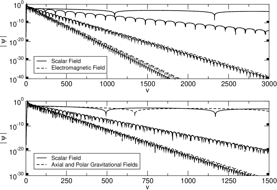
Figure 1: Decay of the scalar and electromagnetic fields with $\ell=1$, and of the scalar, axial and polar gravitational fields, with $\ell=2$, with the SdS geometry approaching the near extreme limit.The parameters for the geometry are $m=1.0$ and $\bar{\delta}=0.01,0.1,0.3$.

Direct calculation of the wave functions confirms that, in the near extreme limit, the dynamics is simple, with the late time decay of the fields being dominated by quasinormal modes. All the types of perturbation tend to coincide near the extreme limit. Besides, as we approach the extreme limit, the oscillation period increases and the exponential decay rate decreases. These conclusions, illustrated in figure 1, for $\ell=1,2$, are consistent with the presented in Cardoso-03 ; Molina-03 .

By using a non-linear fitting based in a $\chi^{2}$ analysis, it is possible to estimate the real and imaginary parts of the $n=0$ quasinormal mode. These results can be compared with the analytical expressions in the near extreme cases. In the figure 2, we analyze the dependence of the frequencies with $\ell$. The accordance is extremely good.

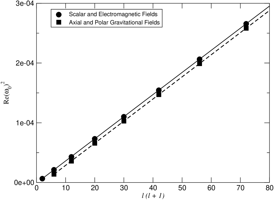
Figure 2: Curve of $Re(\omega_{0})^{2}$ with $\ell(\ell+1)$, for the scalar, electromagnetic and gravitational fields, in the near extreme limit. The dots are the numerical results and the solid lines represent the analytical results. The parameters for the geometry are $m=1.0$ and $\bar{\delta}=0.01$.

V Intermediary Region in Parameter Space

V.1 Scalar Field with $\ell=0$

Only scalar perturbations can have zero total angular momentum. Solutions of (10) with $\ell=0$ leads to a constant tail, as already shown in Brady-97 . This is confirmed in figure 3. The novelty here is the dependence of the asymptotic value on the $\dot{\psi}_{\ell}(0,x)$ initial condition. Figure 3 reveals the appearance of the constant value $\phi_{0}$ for large $t$, and its dependence on $\dot{\psi}_{\ell}(0,x)$. Note that $\phi_{0}$ falls below $10^{-7}$ for $\dot{\psi}_{\ell}(0,x)=0$. These results are in accordance with the analytical predictions of Brady-99 , which give

$$\psi\left(\infty,r\right)=\frac{r}{r_{c}^{2}}\int_{0}^{r_{c}}\dot{\psi}(0,s)s\frac{ds}{h^{\prime}(s)}.$$ (34)

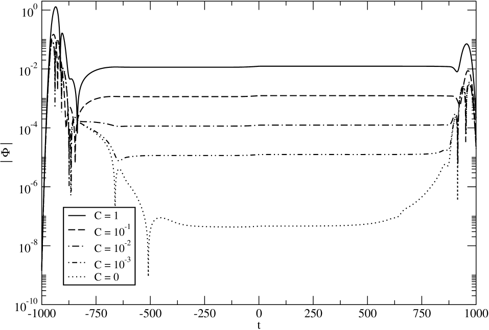
Figure 3: Asymptotic solutions $\Phi(x,t)$ obtained by non-characteristic numerical integration with $\ell=0$, $\Lambda=10^{-4}$ and $m=1$. The curves correspond to different values of $C$ in the initial condition (23).

V.2 Fields with $\ell>0$

We can have scalar and vector fields with angular momentum $\ell=1$, and with $\ell>1$, it is possible to introduce also gravitational fields. Their behavior is described in general by three phases. The first corresponds to the quasinormal modes generated from the presence of the black hole itself. A little later there is a region of power-law decay, which continues indefinitely in an asymptotic flat space. In the presence of a positive cosmological constant, however, an exponential decay takes over in the latest period.

Some qualitatively different effects show up when we turn away from the near extreme limit. For a small cosmological constant the asymptotic behavior is dominated by an exponential decaying mode rather than by a quasinormal mode. Such exponential decays will characterize the de Sitter space in general. We will later comment about the pure de Sitter limit, which is exactly solvable, though we do not have definite answers about the respective behavior. The exponential decay also characterizes the electromagnetic as well as the gravitational perturbations.

As the separation of the horizons increases, the quasinormal frequencies deviate from the predicted by expressions (32) and (33). In figure 4, this is illustrated for $\ell=1,2$.

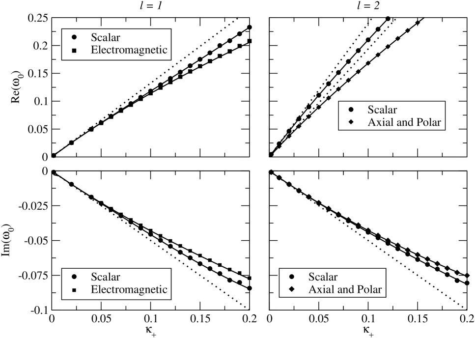
Figure 4: Graphs of the real and imaginary part of the fundamental frequencies $(n=0)$ with $\kappa_{+}$. The dotted lines are the near extreme results, the dots are the numerical results and the continuous curves are the semi-analytic results. In the graphs, $m=1.0$.

It is interesting to compare the values obtained for the fundamental modes using the numerical and semi-analytic methods. We find that the agreement between then is good, for the hole range of $\Lambda$. The difference is better for the first values of $\ell$. This is expected, since the numerical calculations are better in this region. In the table 1, we illustrate these observations with a few values of $\Lambda$. It is important to mention that quasinormal frequencies for the SdS black hole were already calculated in a recent paper Zhidenko , applying a variation of the WKB method used here Konoplya-03 . There are earlier papers calculating quasinormal modes in this geometry, for example dsqnm .

		Numerical		Semi-analytical
$\ell$	$\Lambda$	Re($\omega$)	-Im($\omega$)	Re($\omega$)	-Im($\omega$)
1	1.000E-5	2.930E-01	9.753E-01	2.911E-01	9.780E-02
	1.000E-4	2.928E-01	9.764E-02	2.910E-01	9.797E-02
	1.000E-3	2.914E-01	9.726E-02	2.896E-01	9.771E-02
	1.000E-2	2.770E-01	9.455E-02	2.753E-01	9.490E-02
	1.000E-1	8.159E-02	3.123E-02	8.144E-02	3.137E-02
2	1.000E-5	4.840E-01	9.653E-02	4.832E-01	9.680E-02
	1.000E-4	4.833E-01	8.948E-02	4.830E-01	9.677E-02
	1.000E-3	4.816E-01	8.998E-02	4.809E-01	9.643E-02
	1.000E-2	4.598E-01	8.880E-02	4.592E-01	9.290E-02
	1.000E-1	1.466E-01	3.068E-02	1.466E-01	3.070E-02
3	1.000E-5	6.769E-01	8.662E-02	6.752E-01	9.651E-02
	1.000E-4	6.754E-01	8.654E-02	6.749E-01	9.647E-02
	1.000E-3	6.732E-01	8.660E-02	6.720E-01	9.611E-02
	1.000E-2	6.437E-02	9.200E-02	6.428E-02	9.235E-02
	1.000E-1	2.091E-02	3.054E-02	2.091E-02	3.056E-02

Table 1: Fundamental frequency ($n=0$) of the scalar field, obtained using the numerical and semi-analytical methods. In this table, $m=1.0$.

		Numerical		Semi-analytical
$\ell$	$\Lambda$	Re($\omega$)	-Im($\omega$)	Re($\omega$)	-Im($\omega$)
1	1.000E-5	2.481E-01	9.226E-02	2.459E-01	9.310E-02
	1.000E-4	2.481E-01	9.223E-02	2.457E-01	9.307E-02
	1.000E-3	2.475E-01	9.176E-02	2.448E-01	9.270E-02
	1.000E-2	2.374E-01	8.839E-02	2.352E-01	8.896E-02
	1.000E-1	8.035E-02	3.027E-02	8.023E-02	3.033E-02
2	1.000E-5	4.577E-01	8.985E-02	4.571E-01	9.506E-02
	1.000E-4	4.575E-01	8.991E-02	4.569E-01	9.502E-02
	1.000E-3	4.559E-01	9.439E-02	4.551E-01	9.464E-02
	1.000E-2	4.371E-01	8.941E-02	4.364E-01	9.074E-02
	1.000E-1	1.458E-01	3.037E-02	1.458E-01	3.038E-02
3	1.000E-5	6.578E-01	8.365E-02	6.567E-01	9.563E-02
	1.000E-4	6.576E-01	8.349E-02	6.564E-01	9.559E-02
	1.000E-3	6.547E-01	8.399E-02	6.538E-01	9.520E-02
	1.000E-2	6.276E-02	8.852E-02	6.267E-01	9.125E-02
	1.000E-1	2.085E-02	3.039E-03	2.085E-01	3.040E-02

Table 2: Fundamental frequency ($n=0$) of the electromagnetic field, obtained using the numerical and semi-analytical methods. In this table, $m=1.0$.

		Numerical		Semi-analytical
$\ell$	$\Lambda$	Re($\omega$)	-Im($\omega$)	Re($\omega$)	-Im($\omega$)
2	1.000E-5	3.738E-01	8.883E-02	3.731E-01	8.921E-02
	1.000E-4	3.737E-01	8.880E-02	3.730E-01	8.918E-02
	1.000E-3	3.721E-01	8.850E-02	3.715E-01	8.888E-02
	1.000E-2	3.566E-01	8.538E-02	3.560E-01	8.572E-02
	1.000E-1	1.179E-01	3.020E-02	1.179E-01	3.023E-02
3	1.000E-5	5.999E-01	8.677E-02	5.992E-01	9.272E-02
	1.000E-4	5.996E-01	8.676E-02	5.990E-01	9.269E-02
	1.000E-3	5.972E-01	8.971E-02	5.966E-01	9.234E-02
	1.000E-2	5.725E-01	8.695E-02	5.718E-01	8.874E-02
	1.000E-1	1.900E-01	3.030E-02	1.900E-02	3.032E-02
4	1.000E-5	8.106E-01	8.810E-02	8.091E-01	9.417E-02
	1.000E-4	8.102E-01	8.781E-02	8.087E-01	9.413E-02
	1.000E-3	8.070E-01	8.799E-02	8.055E-01	9.376E-02
	1.000E-2	7.733E-02	8.714E-02	7.720E-01	9.000E-02
	1.000E-1	2.564E-02	3.034E-03	2.563E-01	3.036E-02

Table 3: Fundamental frequency ($n=0$) of the axial and polar gravitational fields, obtained using the numerical and semi-analytical methods. In this table, $m=1.0$.

The first higher $n$ modes cannot be obtained from the numerical solution, but can be calculated by the semi-analytical method. As the cosmological constant decreases, the real and imaginary parts of the frequencies increase, up to the limit where the geometry is asymptotically flat. The behavior of the modes is illustrated in figure 5. The behavior of the electromagnetic field is similar.

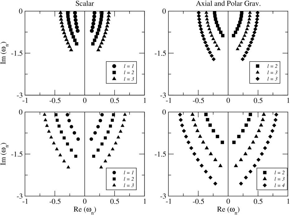
Figure 5: Quasinormal modes of the scalar, axial and polar gravitational fields, for higher modes. The parameter for the curves are $m=1$ and $\Lambda=10^{-3}$.

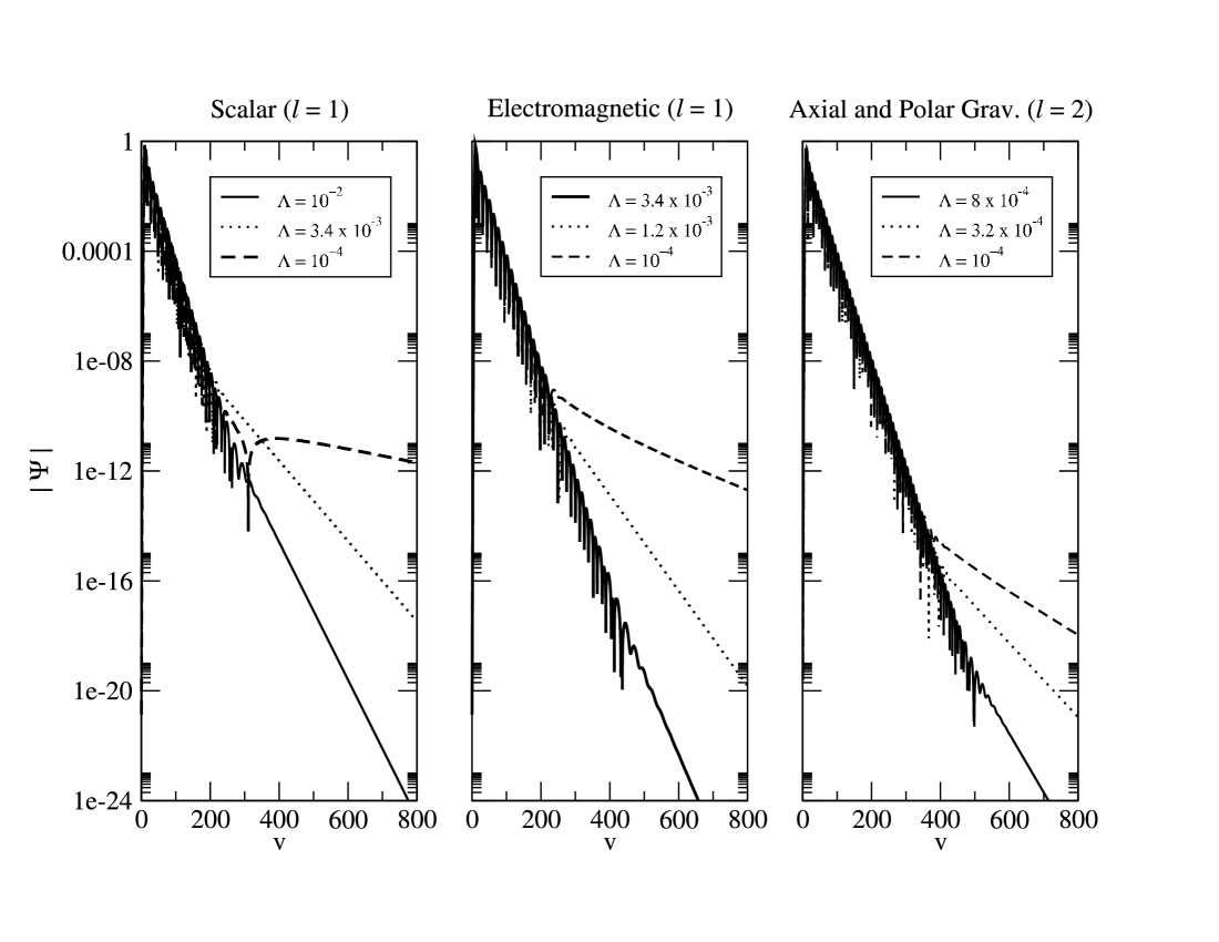
Figure 6: Exponential tail for the scalar and electromagnetic fields with $\ell=1$, and for the axial and polar gravitational field with $\ell=2$. In the graphs, $m=1.0$.

A $\chi^{2}$ analysis of the data presented in figure 6 shows that the massless scalar, electromagnetic and gravitational perturbations in SdS geometry behave as

$$\psi_{\ell}^{sc}\sim e^{-k_{exp}^{sc}t} {\rm with} t\rightarrow\infty$$ (35)

$$\psi_{\ell}^{el}\sim e^{-k_{exp}^{el}t} {\rm with} t\rightarrow\infty$$ (36)

$$\psi_{\ell}^{ax}\sim e^{-k_{exp}^{ax}t} {\rm with} t\rightarrow\infty$$ (37)

$$\psi_{\ell}^{po}\sim e^{-k_{exp}^{po}t} {\rm with} t\rightarrow\infty$$ (38)

for $t$ sufficiently large. At the event and the cosmological horizons $t$ is substituted, respectively by $v$ and $u$.

The numerical simulations developed in the present work reveal an interesting transition between oscillatory modes and exponentially decaying modes. As shown in figure 7, as the cosmological constant decreases, the absolute value of $-\textrm{Im}(\omega)$ decreases.

Above a certain critical value of $\Lambda$ we do not observe the exponential tail, since the coefficient $k_{exp}$ is larger than $-\textrm{Im}(\omega_{0})$ thus the decaying quasinormal mode dominates. But for $\Lambda$ smaller than this critical value, $-\textrm{Im}(\omega_{0})$ turns out to be larger than $k_{exp}$ and the exponential tail dominates. Certainly, for a small enough cosmological constant the exponential tail dominates in the various cases considered here.

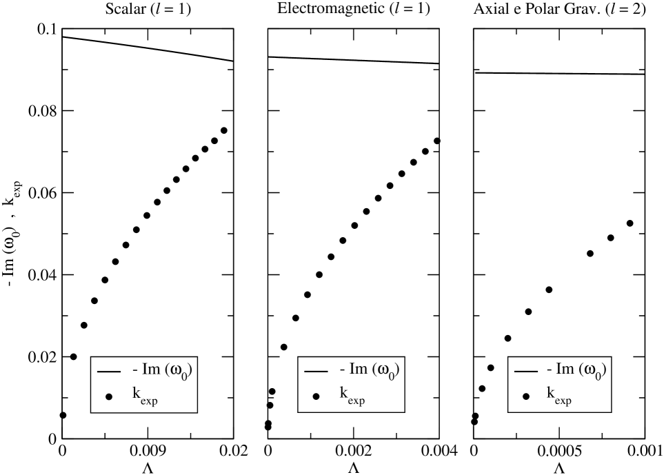
Figure 7: Approaching of the constants $-\textrm{Im}(\omega_{0})$ and $k_{exp}$, for the scalar, electromagnetic and gravitational fields, in the SdS geometry. Above a certain critical value of $\Lambda$ (roughly $1.7\times 10^{-2}$, $4.0\times 10^{-3}$ and $1.2\times 10^{-3}$ respectively, for the parameters taken in graphs), a tail it is not observed. For all curves, the mass is set to $m=1.0$.

Another aspect worth mentioning in the intermediate region is the dependence of the parameters $k_{exp}^{sc}$, $k_{exp}^{el}$, $k_{exp}^{ax}$ and $k_{exp}^{po}$ with $\ell$ and $\kappa_{c}$. The results suggest that the $k_{exp}$ are at least second differentiable functions of $\kappa_{c}$. Therefore, close to $\kappa_{c}=0$, we approximate

$$k_{exp}^{sc}(\kappa_{c})\approx\ell\left(\kappa_{c}+c^{sc}\kappa_{c}^{2}\right)\ ,$$ (39)

$$k_{exp}^{el}(\kappa_{c})\approx k_{exp}^{ax}(\kappa_{c})\approx k_{exp}^{po}(\kappa_{c})\approx(\ell+1)\left(\kappa_{c}+c^{e-g}\kappa_{c}^{2}\right)\ .$$ (40)

Previous results are illustrated in figure 8.

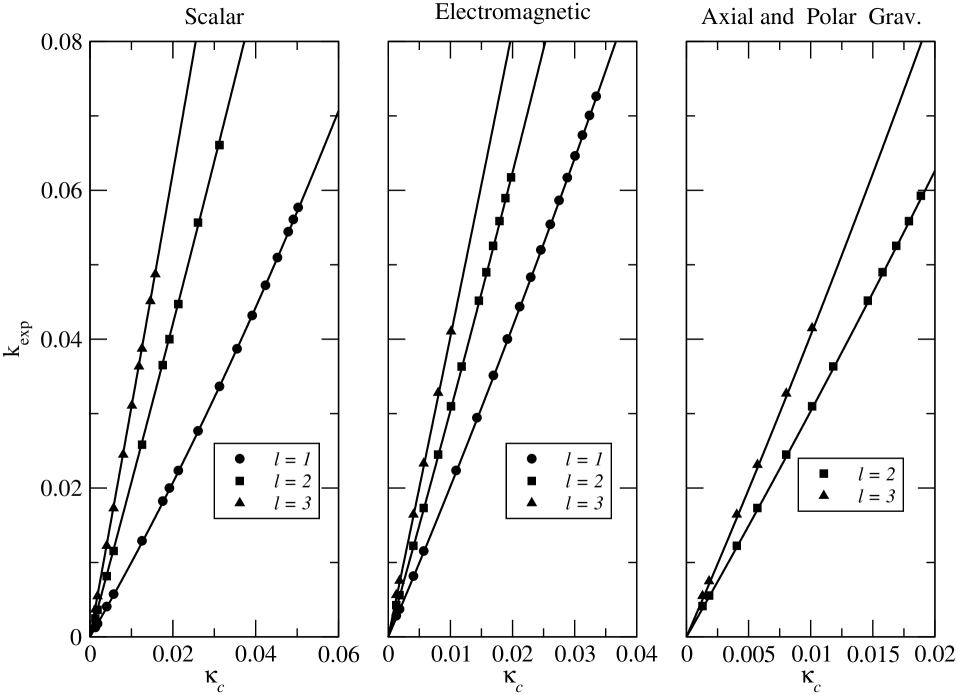
Figure 8: Dependence of $k_{exp}$ with $\kappa_{c}$ and $\ell$, in the SdS geometry. The symbols indicate the numerical values, and the solid lines are the appropriate fittings. For the left graph: $k_{exp}^{sc}=1.077\times 10^{-4}+0.984\kappa_{c}+3.545\kappa_{c}^{2}$, $k_{exp}^{sc}=-1.863\times 10^{-4}+2.010\kappa_{c}+2.608\kappa_{c}^{2}$ and $k_{exp}^{sc}=-1.959\times 10^{-4}+3.028\kappa_{c}+2.978\kappa_{c}^{2}$. For the center graph: $k_{exp}^{el}=2.082\times 10^{-4}+1.988\kappa_{c}+6.141\kappa_{c}^{2}$, $k_{exp}^{el}=2.712\times 10^{-4}+2.974\kappa_{c}+8.284\kappa_{c}^{2}$ and $k_{exp}^{el}=3.737\times 10^{-4}+3.984\kappa_{c}+4.517\kappa_{c}^{2}$. For the right graph: $k_{exp}^{ax}=2.616\times 10^{-4}+2.974\kappa_{c}+9.895\kappa_{c}^{2}$ and $k_{exp}^{ax}=4.484\times 10^{-4}+3.896\kappa_{c}+18.92\kappa_{c}^{2}$. In the graphs, $m=1.0$.

VI Approaching the Asymptotically Flat Geometry

Scalar fields in the SdS geometry near the asymptotically flat limit wore studied in Brady-97 ; Brady-99 . In this case there is a clear separation between the event and the cosmological horizons, such that

$$\delta=\frac{r_{c}-r_{+}}{r_{+}}\gtrsim 50\ .$$ (41)

A new qualitative change occurs in this regime, namely a decaying phase with a power-law behavior. Such a phase occurs between the quasinormal mode decay and the exponential decay phases. The field cannot be simply described by a superposition of the various modes, which would imply a domination of the power-law phase. This is illustrated in figure 9.

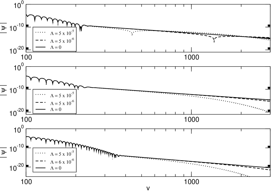
Figure 9: Approaching the asymptotically flat geometry. Straight lines in the log-log graphs indicate power-law decay. In the graphs, $m=1.0$.

VII Conclusions

We have identified three regimes, according to the value of $\Lambda$ for the decay of the scalar, electromagnetic and gravitational perturbations. Near the extreme limit (high $\Lambda$), we have analytic expressions for the effective potentials and to the quasinormal frequencies. The decay is entirely dominated by the quasinormal modes, that is, oscillatory decaying characterized by a non vanishing real part of the quasinormal frequency.

In an intermediary parameter region (lower $\Lambda$), the wave functions have an important qualitative change, with the appearance of an exponential tail. This tail dominates the decay for large time. Near the asymptotically flat limit ($\Lambda\ll 1$), we see an intermediary phase between the quasinormal modes and the exponential tail — a region of power-law decay. When $\Lambda=0$, this region entirely dominates the late time behavior.

Finally, for scalar fields with $\ell=0$ a constant decay mode appears, and its value depends on the $\dot{\psi}_{\ell}(0,x)$ initial condition. Figure 3 reveals the appearance of the constant value $\phi_{0}$ for large $t$, and its dependence on $\dot{\psi}_{\ell}(0,x)$. The value of $\phi_{0}$ falls below $10^{-7}$ for $\dot{\psi}_{\ell}(0,x)=0$.

An immediate extension of the work developed in this paper is the in treatment of field propagation in the exterior of charged and asymptotically de Sitter black holes. In this case, the electromagnetic and gravitational perturbations are necessarily coupled. It would be interesting to see if the general picture presented here is still valid in this more general context.

- (1) T. Regge and J.A. Wheeler, Phys. Rev. 108, 1063 (1957).
- (2) S. Chandrasekhar, The Mathematical Theory of Black Holes, (Oxford University Press, Oxforf, 1983).
- (3) K. D. Kokkotas and B. G. Schmidt, Living Rev. Relativity 2 (1999), gr-qc/9909058.
- (4) A. Riess et al. Astrophy. J. 116, 1009 (1998), astro-ph/9805201; S. Perlmutter et al., Astrophys. J. 517, 565 (1999), astro-ph/9812133.
- (5) V. Cardoso and J. P. S. Lemos, Phys. Rev. D 64, 084017 (2001), gr-qc/0105103.
- (6) B. Wang, C. Lin and E. Abdalla, Phys. Lett. B, 481, 79 (2000), hep-th/0003295; R. A. Konoplya, Phys. Rev. D 66, 044009 (2002), hep-th/0205142; E. Berti and K. D. Kokkotas, Phys. Rev. D 67, 064020 (2003), gr-qc/0301052; V. Cardoso, R. Konoplya and J. P. S. Lemos, Phys. Rev. D 68, 044024 (2003), gr-qc/0305037.
- (7) V. Cardoso and J. P. S. Lemos, Class. Quant. Grav. 18, 5257 (2001), gr-qc/0107098; V. Cardoso and J. P. S. Lemos, Phys. Rev. D 63, 124015 (2001), gr-qc/0101052; J. M. Zhu, B. Wang and E. Abdalla, Phys. Rev. D 63, 124004 (2001), hep-th/0101133; B. Wang, E. Abdalla and R. B. Mann, Phys. Rev. D 65, 084006 (2002), hep-th/0107243.
- (8) B. Wang, C. Molina and E. Abdalla, Phys. Rev. D 63, 084001 (2001), hep-th/0005143.
- (9) H. Nariai, Sci. Rep. Tohoku Univ. 34, 160 (1950); H. Nariai, Sci. Rep. Tohoku Univ. 35, 62 (1951).
- (10) E. W. Leaver, Phys. Rev. D 34, 384 (1986).
- (11) E. S. C. Ching, P. T. Leung, W. M. Suen and K. Young, Phys. Rev. D 52, 2118 (1995), gr-qc/9507035.
- (12) G. Gamow, Zeits. F. Phys. 51 204 (1928).
- (13) P. R. Brady, C. M. Chambers, W. Krivan and P. Laguna, Phys. Rev. D 55, 7538 (1997), gr-qc/9611056.
- (14) P. R. Brady, C. M. Chambers, W. G. Laarakkers and E. Poisson, Phys. Rev. D 60, 064003 (1999), gr-qc/9902010.
- (15) B. F. Schutz and C. M. Will, Astrophys. J. 291, L33 (1985).
- (16) S. Iyer and C. M. Will, Phys. Rev. D 35, 3621 (1987).
- (17) S. Iyer, Phys. Rev. D 35, 3632 (1987); K. D. Kokkotas and B. F. Schutz, Phys. Rev. D 37, 3378 (1988).
- (18) R. A. Konoplya, Phys. Rev. D 68, 024018 (2003), gr-qc/0303052.
- (19) A. Zhidenko, Quasi-normal modes of Schwarzschild-de Sitter black holes, gr-qc/0307012.
- (20) S. Yoshida and T. Futamase, Numerical analysis of quasinormal modes in nearly extremal Schwarzschild-de Sitter spacetimes, gr-qc/0308077.
- (21) E. Abdalla, B. Wang, A. Lima-Santos and W.G. Qiu, Phys. Lett. B 538, 435 (2002), hep-th/0204030; E. Abdalla, K.H.C. Castello-Branco, A. Lima-Santos, Mod. Phys. Lett. A 18, 1435 (2003), gr-qc/0301130.
- (22) R. Ruffini, J. Tiomno and C. Vishveshwara, Lettere al Nuovo Cimento 3, 211 (1972).
- (23) C. Gundlach, R. Price and J. Pullin, Phys. Rev. D 49, 883 (1994).
- (24) R. Price, Phys. Rev. D 5, 2419 (1972).
- (25) A.R. Levander, Geophysics 53, 1425 (1988).
- (26) V. Cardoso and J. P. S. Lemos, Phys. Rev. D 67, 084020 (2003), gr-qc/0301078.
- (27) C. Molina, Phys. Rev. D 68, 064007 (2003), gr-qc/0304053.
- (28) H. Otsuki and T. Futamase, Prog. Theor. Phys. 85, 771 (1991); I. Moss and J. Norman, Class. Quant. Grav. 19, 2323 (2002).