Chaos around charged black hole with dipoles

Abstract

We investigated dynamics of the test particle in the gravitational field of the charged black hole with dipoles in this paper. At first we have studied the gravitational potential, by the numerical simulations, we found, for appropriate parameters, that there are two different cases in the potential curve, one is a well case with a stable critical point, and the other is three wells case with three stable critical points and two unstable critical points. As consequence, the chaotic motion will rise. We have performed the evolution of the orbits of the test particle in phase space, we found that the orbits of the test particle randomly oscillate without any periods, even sensitively depend on the initial conditions and parameters. By performing Poincaré sections for different values of the parameters and initial condition, we have found regular motion and chaotic motion. By comparing these Poincaré sections, we further conformed that the chaotic motion of the test particle mainly origins from the dipoles of the black hole.

I Introduction

Chaotic behaviors were considered as a interesting phenomena by many physicists since Lorenz found the deterministic non-periodic flowlorenz . In the last decades, chaos is one of the most important idea used to explain various nonlinear phenomena in nature. After the research on the three-body problem by Poincaré, many studies about chaos in celestial mechanics and astrophysics have been done and also have found the important role of chaos in the universeMoser wisdom . There are two main lines of research in general relativity, on deals with chaoticity associated with inhomogeneous cosmological models, for example, Oliveira et aloliveira Monerat Tonini Ozorio have studied the chaotic behavior in Bianchi IX model. The other assumes a given metric and looks for chaotic behavior of geodesic motion in this background. Although we know many features of chaos in Newtonian dynamics, we don’t know, so far, so much about those in general relativity. Because the gravitational field around a black hole is very strong and nonlinear, we expect to find a new type of chaotic behavior in such strong gravitational field which does not appear in Newtonian dynamics Misner Belinskii Barrow . Some authors Soota Contopoulos Dettmann Yustsever Karas Varvoglis Bombelli Moeckel Letelier found chaotic behavior of a test particle in relativistic system. Letelier et al Gueron Vieira Letelie investigated the chaos in black hole with halos. J.H. Chen and Y.J.Wang Chen investigated the dynamics of a extreme charged black hole; A. Saa Saa1 Saa2 extended investigation on the integrability of oblique orbits of test particle under the gravitational field corresponding to the superposition of an infinitesimally thin disk and a monopole to the more realistic case, for astrophysical purpose, of a thick disk. And there are many examples in the literature of chaotic motion involving black holes, in the fixed two centers problem Contopoulos Contopoulos1 Cornish , in a black hole surround by gravitational wavesBombelli1 , Leteli , and in several core-shell models with relevance to the description of galaxiesVieira1 . As to Newtonian case, the recent works of C. Chicone et al Chicone on the chaotic behavior of the Hill system. In order to investigate the chaotic behavior of the dynamics system, Many researchers concentrated on the study of chaotic dynamics in general relativity with the Poincaré-Melnikov method Melnikov Wiggins .The Melnikov method is an analytical criterion to determine the occurrence of chaos in integrable systems in which homoclinic (or heteroclinic) manifolds biasymptotic to unstable critical points or to periodic orbits (more generally to invariant tori) are subjected to small perturbations.
It’s well known that the charge non-spheral-symmetry distribution of the charged black hole is a popular phenomena. so it is interested to investigate the motion of the test particle in the space-time of the charged black hole with dipoles. In this paper, by performing the numeral simulations, we figured out orbital evolution in phase space and Poincaré sections for different initial conditions. we confirm that there are regular and chaotic motion of the test particle in the gravitational field of the charged black hole with dipoles. The others organize as follows: In the next section we investigate the Hamiltonian of the charged black hole with dipoles, In section III, we perform the numerical stimulations to study the potential and the evolution of the orbits of the test particle, at the same time we present Poinccaré sections for different parameters. In the last section, a brief conclusion is given.

II Hamiltonian of the charged black hole with dipoles

Wang et alwang1 wang2 wang3 gave out the metric of the charged black hole with dipoles. because the space-time of our system is static axial-symmetry, by using cylindrical $(r,\theta,z)$ to describe the space-time, we obtain the potential which describe the gravitational field of charged black hole with dipoles

$$V=-\frac{M}{\sqrt{r^{2}+z^{2}}}+\frac{Q^{2}}{2(r^{2}+z^{2})}+\frac{P^{2}z^{2}}{2(r^{2}+z^{2})^{3}},$$ (1)

where $M,Q,P$ are mass, charges and dipoles of the black hole, respectively, and $r^{2}+z^{2}=x^{2}+y^{2}+z^{2}$, where $x,y,z$ are the usual Cartesian coordinates.
we know that the angular momentum $L$ in $z$ direction is conserved and we can also easily reduce the three-dimensional original problem to a two-dimensional one in the coordinates $(r,z)$. Now we consider the bounded orbit for the test particle under the potential (1), so the Hamiltonian is

$$H=\frac{\dot{r}^{2}+\dot{z}^{2}}{2}+\frac{L^{2}}{2r^{2}}-\frac{M}{\sqrt{r^{2}+z^{2}}}+\frac{Q^{2}}{2(r^{2}+z^{2})}+\frac{P^{2}z^{2}}{2(r^{2}+z^{2})^{3}}.$$ (2)

The Hamiltonian (2) is smooth everywhere, the corresponding Hamiltonian-Jacobi equations can be properly separated in parabolic coordinates Dorizzi Grammaticos , leading to the second constant of the motion

$$C=R_{z}-\alpha\frac{r^{2}}{2},$$ (3)

where $R_{z}$ is the $z$ component of the Laplace-Runge-Lenz vector

$$R=\frac{M}{\sqrt{r^{2}+z^{2}}}(r\hat{r}+z\hat{z})+V\times L,$$ (4)

where $L$ stands for the total angular momentum. In this case, with two constants of motion $H$ and $C$, the equations for the trajectories of the test particle can be reduced to quadrature in parabolic coordinates Dorizzi Grammaticos and we notice that the equation of motion are invariant under the following rescaling:

$$r\rightarrow\lambda r,z\rightarrow\lambda z,t\rightarrow\lambda t,M\rightarrow\lambda M,$$

$$Q\rightarrow\lambda Q,P\rightarrow\lambda P,H\rightarrow\lambda H.$$ (5)

III Numerical simulations

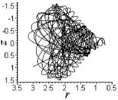
Figure 4: 2Dimesional(r, z) plot of the evolution of the orbit of the test particle in the charged black hole with dipoles in the phase space for $M=1,L^{2}=0.4,P^{2}=12$, $Q^{2}=0.2$ and $H=-0.27800554$.

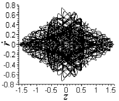
Figure 5: 2Dimesional( ṙ, z) plot of the evolution of the orbit of the test particle in the charged black hole with dipoles in the phase space for $M=1,L^{2}=0.4,P^{2}=12$, $Q^{2}=0.2$ and $H=-0.27800554$.

The gravitational potential (1) changes from one well to three wells when we change one parameter while fixed the other parameters. Fig.1 shows the potential for different values of $P$ ($P^{2}=7(dashed)$ and $P^{2}=2$)(real) with fixed other parameters ($M=1,Q^{2}=0.2,r=1$,). From Fig.1 we can see that the motion in one well is oscillation, however in the three wells potential, the motion is very different from the case of one well case, there are three stable critical points (A) and two unstable critical points (B), when the kinetic energy of the test particle is much higher than the gravitational potential, the motion is similar to the one well case, but when the kinetic energy of the test particle is closed to the gravitational potential, the motion oscillate randomly in one of the three wells, particularly near the two unstable critical points, so the motion of the test particle in this case sensitively depending on the initial conditions and the parameters so that it becomes chaotic. The Melnikov method is useful to find the regions of chaotic oscillation. In this paper, we will not use the analytical method,we will figure out the evolution of the test particle in phase space and its Poinccaré section method to investigate the properties of the dynamics of the test particle in the gravitational field of charged black hole with dipoles. Abdullaev1 Abdullaev2 .
In order to investigate the evolutions of the test particle in the gravitational field of the charged black hole with dipoles and its chaotic behavior, we use variables $(\dot{r},\dot{z},r,z)$ and the package POINCARÉCeb-Terrab to perform following numerical experiments. Figs.2-5 show the evolution of the particle in the compact phase space. We can see that the particle oscillates randomly in the phase space with no periodic and sensitively depends on the initial conditions and the parameters of the system, that’s to say, the properties of the motion is chaotic if we choose properly parameters, which is expected by studying the dynamics of the particle in the gravitational potential of the charged black hole with dipoles.
To determine the chaotic behavior of a dynamical system, we can further perform the Poincaré section in the phase space. If the motion is not chaotic, the plotted points form a closed curve in the two-dimensional $(\dot{r},r)$ plane, because a regular orbit will move on a torus in the phase space and the curve is a cross section of the torus; If the orbit is chaotic, some of those tori will be broken and the Poincaré section does not consist of a set of closed curves, but the points will be distributed randomly in the allowed region to form a chaotic sea. From the distribution of the points in Poincaré section, we can judge whether or not the motion is chaotic. Figs. 6-11 show the typical Poincaré sections across the plane $z=0$ for different initial conditions. In Fig.6, we present the Poincaré section for $M=1,L^{2}=0.4,P^{2}=12$, $Q^{2}=2$ and $H=-0.18800554$, the section consists of KAM tori structure which characterizes a quasi-integrable Hamilton system with quasi-periodic orbits. Under these values of the parameters, there is no chaotic behavior. Then in Fig.7, we plot the Poincaré sections for $M=1,L^{2}=0.4,P^{2}=1.2$, $Q^{2}=0.2$ and $H=-0.28340554$, we can see that some points have distributed randomly in a finite region to form a chaotic sea and there two islands which are surrounded by the chaotic sea. If we go on changing the parameters and the initial conditions to draw Fig.8 for $M=1,L^{2}=0.4,P^{2}=12$, $Q^{2}=0.2$, $H=-0.27800554$ and $M=1,L^{2}=0.2,P^{2}=12$, $Q^{2}=0.2$, $H=-0.28911665$, further larger chaotic sea will obtain in an allowed region and the islands will almost submerge by the chaotic sea, this means that the quasi-periodic orbits change into chaos. By comparing the parameters of Figs.6-9, we can find that chaotic behavior mainly origins from the dipoles of the black hole i.e.the non-sphere-symmetry of the charge distribution in the black hole.
Performing further investigation, we will figure out the two following extreme cases, Fig.10 present Poincaré section for $M=1,L^{2}=0.4,P^{2}=1.2$, $Q^{2}=0$ and $H=-0.29340554$. In this case the black hole is neutron, due to the un-sphere-symmetry of the charge distribution, there are dipoles $P$ in the black hole. From Fig.10, we can find that there are two islands surround by a large chaotic sea, that’s to say, under above parameters our system is chaotic. However if the charges distribute spheral-symmetry in the black hole, there is no dipole , so we figure out Poincaré section for $M=1,L^{2}=0.4,P^{2}=0$, $Q^{2}=0.2$ and $H=-0.28400554$. From Fig.11, we obviously see that there is KAM tori structure in the section, this case corresponds to an integrable motion.

IV Conclusions and discussions

In this paper we investigated the gravitational potential (1), by the numerical stimulations, we find, for appropriate parameters of the our system, that there are two cases in the potential curves, one is a well case with a stable critical point, and the other is three wells case with three stable critical points and two unstable critical points. As consequence, the chaotic motion will rise. In order to verify the chaotic motion, we have performed the evolution of the orbits of the test particle in phase space, we can obviously see that the orbits randomly oscillate without any periods, even sensitively depend on the initial conditions and parameters. By the Poincaré section method, we have presented Poincaré sections for different values of the parameters and initial conditions. In these Poincaré sections we have found regular motion and chaotic motion. By comparing these Poincaré sections, we further conform that the chaotic motion of the test particle mainly origins from the dipoles of the black hole.

V Acknowledgments

Authors are very grateful for the helps of Professor Alberto Saa (Departamento de Matem$\acute{a}$tica Aplicada, IMECC-UNICANP Campinas. S.P. Brazil ), Professor H. P. de Oliveira (NASA/Fermilab Astrophysics Center, Fermi National Accelaratory Batavia, $\Pi$linois) and Professor Wenhua Hai, Professor Jiliang Jing, Professor Hongwei Yu (Department of Physics, Hunan Normal University, People Republic of China).

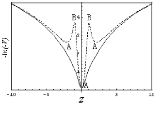
Figure 1: Plots of Gravitational potential (1) for $M^{2}=1,Q^{2}=0.2,r=1$ and $P^{2}=7$ (dashed), $2$ (real). From the plots we can see that when $P^{2}=2$ (real) there only one well in the potential curve and a stable critical point (A); but when $P^{2}=7$ (dashed) there are three wells in the potential curve and three stable critical points (A) and two unstable critical points (B). the test particle oscillates randomly in one of three wells.

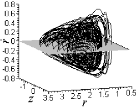
Figure 2: 3Dimesional(ṙ, r, z) plot of the evolution of the orbit of the test particle in the charged black hole with dipoles in the phase space for $M=1,L^{2}=0.4,P^{2}=12$, $Q^{2}=0.2$ and $H=-0.27800554$.

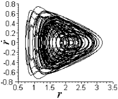
Figure 3: 2Dimesional(ṙ, r) plot of the evolution of the orbit of the test particle in the charged black hole with dipoles in the phase space for $M=1,L^{2}=0.4,P^{2}=12$, $Q^{2}=0.2$ and $H=-0.27800554$.

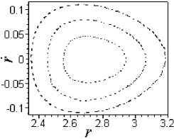
Figure 6: Pioncaré section (ṙ, r) across the plane $z=0$, ż $>$ 0 for $M=1,L^{2}=0.4,P^{2}=12$, $Q^{2}=2$ and $H=-0.18800554$. For these values of the parameters we have the section of an integrable motion.

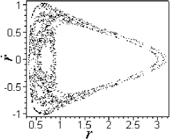
Figure 7: Pioncaré section (ṙ, r) across the plane $z=0$, ż $>$ 0 for $M=1,L^{2}=0.4,P^{2}=1.2$, $Q^{2}=0.2$ and $H=-0.28340554$. Under these conditions there is a large chaotic sea, which means chaotic motion of the test particle, in the section.

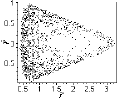
Figure 8: Pioncaré section (ṙ, r) across the plane $z=0$, ż $>$ 0 for $M=1,L^{2}=0.4,P^{2}=12$, $Q^{2}=0.2$ and $H=-0.27800554$. Under these conditions there is a larger chaotic sea, which means chaotic motion of the test particle, than the precedent figure in the section.

Figure 9: Pioncaré section (ṙ, r) across the plane $z=0$, ż $>$ 0 for $M=1,L^{2}=0.2,P^{2}=12$, $Q^{2}=0.2$ and $H=-0.28911665$. Under these conditions there is a much larger chaotic sea, which means chaotic motion of the test particle, than the precedent two figures in the section.

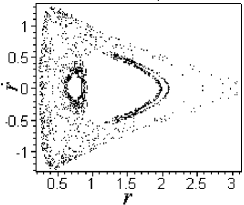
Figure 10: Pioncaré section (ṙ, r)across the plane $z=0$, ż $>$ 0 for $M=1,L^{2}=0.4,P^{2}=1.2$, $Q^{2}=0$ and $H=-0.29340554$. Under these extreme conditions there is large chaotic sea, which means chaotic motion of the test particle, in the section.

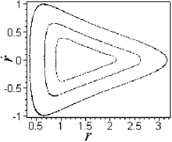
Figure 11: Pioncaré section (ṙ, r)across the plane $z=0$, ż $>$ 0 for $M=1,L^{2}=0.4,P^{2}=0$, $Q^{2}=0.2$ and $H=-0.28400554$. For these extreme values of the parameters we have the section of an integrable motion just as Fig.6.

References

- (1) Lorenz E.N., J. Atoms. Sci. 20 (1963)
- (2) T. Moser,Math. Intelligencer 1, 65 (1978)
- (3) J. Wisdom, Proc. R. Soc. London A413, 109 (1987)
- (4) H. P. de Oliveira, I. Damiao Soares and T. J. Stuchi, Phys. Rev. D56, 730 (1997)
- (5) G. A. Monerat, H. P. de Oliveira and I. Damiao Soares, Phys. Rev. D58, 063504 (1998)
- (6) E. V. Tonini, Phys. Rev. D63, 063502 (2001)
- (7) H. P. de Oliveira, A.M. Ozorio de Almeida, I. Damiao Soares and E. V. Tonini, gr-qc/0202047
- (8) C. W. Misner, Phys. Rev. Lett. 22 1071 (1969)
- (9) V. A. Belinskii, I. M. Khalatnikov and E. M. Lifshitz, Adv. Phys. 19, 525 (1970)
- (10) J.D. Barrow, Phys. Rep. 85, 1 (1982)
- (11) Y. Soota, S. Suzuki and K. Maeda, Class. Quantum. Grav. 13, 1241 (1996)
- (12) G. Contopoulos, Proc. R. Soc. London A435, 551 (1991)
- (13) C. P. Dettmann, N. E. Frankel and N. J. Cornish, Phys. Rev. D50 R618 (1994)
- (14) U. Yustsever, Phys. Rev. D52, 3176 (1995)
- (15) V. Karas and D. Vokrouhlický, Gen. Relativ. Gravit. 24, 729 (1992)
- (16) H. Varvoglis and D. Papadopoulos, Astron. Astrophys. 261, 664 (1992)
- (17) L. Bombelli and E. Calzetta, Class. Quantum Grav. 9, 2573 (1992)
- (18) R. Moeckel, Commun. Math. Phys. 150, 415 (1992)
- (19) P. S. Letelier and W. M. Vieira, Class. Quantum Grav. 14, 1249 (1997)
- (20) E. Guéron and P. S. Letelier, astro-ph/0101140
- (21) W. M. Vieira and P. S. Letelier, Phys. Lett. A228, 22 (1997)
- (22) P. S. Letelier and W. M. Vieira, Phys. Rev. D56, (1997)
- (23) J.H. Chen and Y.J.Wang, Acta. Phys. Sinca, V50, 1833 (2001)
- (24) Alberto. Saa, Phys. Lett. A259, 201 (1999)
- (25) Alberto. Saa, Phys. Lett. A269, 204 (2000)
- (26) G. Contopoulos, Proc. R. Soc. London, A431, 183 (1990)
- (27) N.J. Cornish and G. W. Gibbons, Class. Quantum. Grav. 14, 1865 (1997)
- (28) L. Bombelli and E. Calzetra, Class. Quantum. Grav. 9, 2573 ( 1992)
- (29) P.S.Letelier and W.M. Vieira, Class. Quantum. Grav. 14, 1249 (1997)
- (30) W.M. Vieira and P.S. Letelier, Astrophys. J, 513, 383 (1999)
- (31) C. Chicone B. Mashhoon, and D.G. Retzloff, Helv, Phys. Acta. 72, 123 (1999)
- (32) V. K. Melnikov, Trans. Moscow. Math. Soc. 12, 1 (1963)
- (33) S. Wiggins, Global Bifurcations and Chaos (New York, Springer 1988)
- (34) Y. J. Wang, Science in China, A44, 801 (2001)
- (35) Y. J. Wang, General Relativity and Cosmology, (Hunan Science and Technology Press, Hunan 2000)
- (36) Y. J. Wang, Y. B. huang, Chin. J. Astron. Astrophys. A1, 125 (2001)
- (37) B. Dorizzi, B. Grammaticos and A. Ramani, J. Math. Phys. 25, 481 (1984)
- (38) B. Grammaticos, B. Dorizzi, A. Ramani and J. Hietarinta, Phys. Lett., 109A, 81 (1985)
- (39) F. Kh. Abdullaev and R. A. Kraenkel, Phys. Rev. A62, 023613 (2000)
- (40) F. Kh. Abdullaev and R. A. Kraenkel, arXiv: e-print cond-mat/0005445 (2000)
- (41) E. S. Ceb-Terrab and H. P. de Oliveira, Comput. Phys. Commun. 95, 171 (1996)