Complex angular momentum in black hole physics and quasinormal modes

Abstract

By using the complex angular momentum approach, we prove that the quasinormal mode complex frequencies of the Schwarzschild black hole are Breit-Wigner type resonances generated by a family of surface waves propagating close to the unstable circular photon (graviton) orbit at $r=3M$. Furthermore, because each surface wave is associated with a given Regge pole of the $S$-matrix, we can construct semiclassically the spectrum of the quasinormal-mode complex frequencies from Regge trajectories. The notion of surface wave orbiting around black holes thus appears as a fundamental concept which could be profitably introduced in various areas of black hole physics in connection with the complex angular momentum approach.

I Introduction

Since the pioneering work of Watson Watson (1918) dealing with the propagation and diffraction of radio waves around the Earth, the complex angular momentum (CAM) method has been extensively used in several domains of scattering theory (see the monographs of Newton Newton (1982) and of Nussenzveig Nussenzveig (1992) and references therein for various applications in quantum mechanics, nuclear physics, electromagnetism, optics, acoustics and seismology). The success of the CAM method is due to its ability to provide a clear description of a given scattering problem by extracting the physical information (linked to the geometrical and diffractive aspects of the scattering process) which is hidden in partial-wave representations.

The CAM method was first used in gravitational physics by Chandrasekar and Ferrari Chandrasekhar and Ferrari (1992) in their study of nonradial oscillations of relativistic stars. They used the theory of Regge poles Newton (1982) to determine the flow of gravitational energy through the star. The general framework for the CAM description of Schwarzschild black hole scattering was developed by Andersson and Thylwe Andersson and Thylwe (1994), which Andersson Andersson (1994) then used to interpret the black hole glory. An important concept, which is naturally present in the CAM point of view, is that of a surface wave, which allows a description of the diffractive effects of scattering. Andersson established that the surface waves orbiting around the Schwarzschild black hole of mass $M$ propagate close to the unstable photon orbit at $r=3M$. Yet except for these articles, the CAM/surface-wave approach to resonant scattering in black hole physics has been neglected in favor of the quasi-normal modes (QNMs), in which the dynamical response to an external perturbation is explained in terms of resonant frequencies. For recent reviews of the QNM approach see Refs. Kokkotas and Schmidt, 1999 and Nollert, 1999 as well as chapter 4 of Ref. Frolov and Novikov, 1998. An introduction to black hole scattering can be found in Andersson and Jensen (gr-qc/0011025).

In this paper we will establish the connection between Andersson’s surface waves and the QNMs. More precisely, we shall prove here that the QNM complex frequencies of the Schwarzschild black hole are Breit-Wigner-type resonances generated by the surface waves. Moreover, because each surface wave is associated with a given Regge pole of the $S$-matrix, we can construct the spectrum of the QNM complex frequencies from the Regge trajectories, i.e., from the curves traced out in the CAM plane by the Regge poles as a function of the frequency.

As early as 1972, it was suggested by Goebel Goebel (1972) that the black hole normal modes could be interpreted in terms of gravitational waves in spiral orbits close to the unstable photon orbit at $r=3M$, which decay by radiating away energy. In the present paper, using the CAM approach, we establish this appealing and physically intuitive picture on a rigorous basis. To conclude, we also provide a framework for future developments.

II From CAM to QNM

We first consider the scattering of a monochromatic scalar wave, with time dependence $\exp(-i\omega t)$, by the Schwarzschild black hole of mass $M$. The corresponding scattering amplitude can be written (see, e.g. Frolov and Novikov (1998))

$$f(\omega,\theta)=\frac{1}{2i\omega}\sum_{\ell=0}^{+\infty}(2\ell+1)\left(S_{\ell}(\omega)-1\right)P_{\ell}(\cos\theta)$$ (1)

where $\ell$ is the ordinary angular momentum index, $P_{\ell}$ are the usual Legendre polynomials and $S_{\ell}$ are the diagonal elements of the $S$-matrix. For a given angular momentum $\ell$, the coefficient $S_{\ell}$ is obtained from the partial wave solution $\Phi_{\ell}$ of the following problem:

(i) $\Phi_{\ell}$ satisfies the Schrödinger-type equation

$$\frac{d^{2}\Phi_{\ell}}{dr_{*}^{2}}+\left[\omega^{2}-V(r)\right]\Phi_{\ell}=0.$$ (2)

Eq. (2) is obtained from the scalar wave equation after separating variables and is called the Regge-Wheeler equation. Here $r$ is the standard radial Schwarzschild coordinate and $r_{*}=r+2M\ln\left(1-2M/r\right)+\mathrm{const}$ is the Regge-Wheeler tortoise coordinate while the potential $V(r)$ is given by

$$V(r)=\left(\frac{r-2M}{r}\right)\left[\frac{\ell(\ell+1)}{r^{2}}+\frac{2M}{r^{3}}\right].$$ (3)

(ii) $\Phi_{\ell}$, as any physical wave, must have a purely ingoing behavior at the event horizon at $r=2M$, i.e.

$$\Phi_{\ell}(r)\underset{r_{*}\to-\infty}{\sim}e^{-i\omega r_{*}}.$$ (4)

(iii) At spatial infinity $r\to+\infty$, $\Phi_{\ell}$ has the asymptotic behavior

$$\Phi_{\ell}(r)\underset{r_{*}\to+\infty}{\sim}\frac{1}{T_{\ell}(\omega)}e^{-i\omega r_{*}+i\ell\pi/2}-\frac{S_{\ell}(\omega)}{T_{\ell}(\omega)}e^{+i\omega r_{*}-i\ell\pi/2}.$$ (5)

For certain complex values of $\omega$, both $S_{\ell}$ and $T_{\ell}$ have a simple pole but $S_{\ell}/T_{\ell}$ is regular. These values are the frequencies of the QNMs, which we can define (see Eqs. (4) and (5)) as the solutions of the wave equation which represent a purely outgoing wave at infinity and a purely ingoing wave at the horizon. We now denote by $\omega_{\ell n}=\omega^{(o)}_{\ell n}-i\Gamma_{\ell n}/2$ with $\omega^{(o)}_{\ell n}>0$ and $\Gamma_{\ell n}>0$ the QNM frequencies, $\omega^{(o)}_{\ell n}$ representing the frequency of the oscillation corresponding to the QNM and $\Gamma_{\ell n}$ representing its damping. In the immediate neighborhood of $\omega_{\ell n}$, $S_{\ell}(\omega)$ has the Breit-Wigner form, i.e.,

$$S_{\ell}(\omega)\propto\frac{\Gamma_{\ell p}/2}{\omega-\omega^{(o)}_{\ell p}+i\Gamma_{\ell p}/2}.$$ (6)

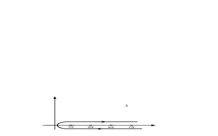
Figure 1: The Watson integration contour.

Using the CAM method, we can provide a physical picture of the scattering process in term of diffraction by surface waves and a physical explanation of the mechanism of QNM excitation valid for high frequencies. By means of a Watson transformation Watson (1918) applied to the scattering amplitude (1), we can write Andersson and Thylwe (1994)

$$f(\omega,\theta)=-\frac{1}{2\omega}\int_{\cal C}\frac{\lambda\left(S_{\lambda-1/2}(\omega)-1\right)}{\cos\pi\lambda}P_{\lambda-1/2}(-\cos\theta)~{}d\lambda.$$ (7)

Here $\mathcal{C}$ is the integration contour in the complex $\lambda$-plane Watson (1918) illustrated in Fig. 1. The Watson transformation permits us to replace the ordinary angular momentum $\ell$ by the complex angular momentum (CAM) $\lambda$. Here $S_{\lambda-1/2}(\omega)$ is now an analytic extension of $S_{\ell}(\omega)$ into the complex $\lambda$-plane which is regular in the vicinity of the positive real $\lambda$ axis. Moreover, $P_{\lambda-1/2}(z)$ is the hypergeometric function $F(-\lambda+1/2,\lambda+1/2;1;(1-z)/2)$.

We can then deform the path of integration in Eq. (7), taking into account the possible singularities. The only singularities that are encountered are the poles of the S-matrix lying in the first quadrant of the CAM plane Andersson and Thylwe (1994). They are known as Regge poles Newton (1982); Nussenzveig (1992) and we shall denote them by $\lambda_{n}(\omega)$, the index $n=1,2,\dots$ permitting us to distinguish between the different poles. By Cauchy’s Theorem we can then extract from Eq. (7) the contribution of a residue series over Regge poles given by

$$f_{P}(\omega,\theta)=\frac{-i\pi}{\omega}\sum_{n=1}^{+\infty}\frac{\lambda_{n}(\omega)r_{n}(\omega)}{\cos\left(\pi\lambda_{n}(\omega)\right)}P_{\lambda_{n}(\omega)-1/2}(-\cos\theta)$$ (8)

where $r_{n}(\omega)=\mathrm{residue}\left(S_{\lambda-1/2}(\omega)\right)_{\lambda=\lambda_{n}(\omega)}$. It should be noted that $f$ differs from $f_{P}$ by a background integral Andersson and Thylwe (1994) which does not play any role in the resonance phenomenon. By using the asymptotic expansion

$$P_{\lambda-1/2}(-\cos\theta)\sim\frac{e^{i\lambda(\pi-\theta)-i\pi/4}+e^{-i\lambda(\pi-\theta)+i\pi/4}}{({2\pi\lambda\sin\theta})^{1/2}}$$

as $|\lambda|\to\infty$, valid for $|\lambda|\sin\theta>1$, as well as

$$\frac{1}{\cos\pi\lambda}=2i\sum_{m=0}^{+\infty}e^{i\pi(2m+1)(\lambda-1/2)}$$

which is true if $\mathrm{Im}\ \lambda>0$, we can write

$$f_{P}(\omega,\theta)=\frac{2\pi}{i\omega}\sum_{n=1}^{+\infty}\frac{\lambda_{n}(\omega)r_{n}(\omega)}{\left[2\pi\lambda_{n}(\omega)\sin\theta\right]^{1/2}}$$

$$\qquad\qquad\times\sum_{m=0}^{+\infty}\left(e^{i\lambda_{n}(\omega)(\theta+2m\pi)-im\pi+i\pi/4}\right.$$

$$\qquad\qquad\qquad\qquad+\left.e^{i\lambda_{n}(\omega)(2\pi-\theta+2m\pi)-im\pi-i\pi/4}\right).\quad$$ (9)

In Eq. (II), terms like $\exp[i\lambda_{n}(\omega)(\theta)]$ and $\exp[i\lambda_{n}(\omega)(2\pi-\theta)]$ correspond to surface wave contributions. Because a given Regge pole $\lambda_{n}(\omega)$ lies in the first quadrant of the CAM plane, $\exp[i\lambda_{n}(\omega)(\theta)]$ (resp. $\exp[i\lambda_{n}(\omega)(2\pi-\theta)]$) corresponds to a surface wave propagating counterclockwise (resp. clockwise) around the black hole and $\mathrm{Re}\ \lambda_{n}(\omega)$ represents its azimuthal propagation constant while $\mathrm{Im}\ \lambda_{n}(\omega)$ is its damping constant. The exponential decay $\exp[-\mathrm{Im}\ \lambda_{n}(\omega)\theta]$ (resp. $\exp[-\mathrm{Im}\ \lambda_{n}(\omega)(2\pi-\theta)]$) is due to continual reradiation of energy. Moreover, in Eq. (II), the sum over $m$ takes into account the multiple circumnavigations of the surface waves around the black hole as well as the associated radiation damping. Finally, the presence of the factor $\exp[-im\pi]$ in Eq. (II) should be also noted: it accounts for the phase advance due to the two caustics on the scattering axis.

The resonant behavior of the black hole can now be understood in terms of surface waves. As $\omega$ varies, each Regge pole $\lambda_{n}(\omega)$ describes a Regge trajectory Newton (1982) in the CAM plane. When the quantity $\mathrm{Re}\ \lambda_{n}(\omega)$ coincides with a half-integer (a half-integer but not an integer because of the caustics), a resonance occurs. Indeed, it is produced by a constructive interference between the different components of the $n$-th surface wave, each component corresponding to a different number of circumnavigations. Resonance wave frequencies $\omega^{(o)}_{\ell n}$ are therefore obtained from the Bohr-Sommerfeld type quantization condition

$$\mathrm{Re}\ \lambda_{n}\left(\omega^{(o)}_{\ell n}\right)=\ell+\frac{1}{2}\qquad\ell=0,1,2,\dots.$$ (10)

By assuming that $\omega$ is in the neighborhood of $\omega^{(o)}_{\ell n}$ and using $\mathrm{Re}\ \lambda_{n}(\omega)\gg\mathrm{Im}\ \lambda_{n}(\omega)$ (which can be numerically verified, except for very low frequencies), we can expand $\lambda_{n}(\omega)$ in a Taylor series about $\omega^{(o)}_{\ell n}$, and obtain

$$\lambda_{n}(\omega)\approx\ell+\frac{1}{2}+\left.\frac{d\ \mathrm{Re}\lambda_{n}(\omega)}{d\omega}\right|_{\omega=\omega^{(o)}_{\ell n}}(\omega-\omega^{(o)}_{\ell n})$$

$$\qquad\qquad+i\ \mathrm{Im}\ \lambda_{n}(\omega^{(o)}_{\ell n}).$$ (11)

Then, by replacing Eq. (II) in the term ${\cos\left(\pi\lambda_{n}(\omega)\right)}$ of Eq. (8), we show that $f_{P}(\omega,\theta)$ presents a resonant behavior given by the Breit-Wigner formula (6) with

$$\frac{\Gamma_{\ell n}}{2}=\left.\frac{\mathrm{Im}\ \lambda_{n}(\omega)}{d\ \mathrm{Re}\ \lambda_{n}(\omega)/d\omega}\right|_{\omega=\omega^{(o)}_{\ell n}}.$$ (12)

Eqs. (10) and (12) are kind of semiclassical formulas which permit us to determine the location of the resonances from Regge trajectories.

We now discuss the numerical aspects of our work. In order to determine the location of the QNM frequencies from Eqs. (10) and (12), we need the Regge trajectories. For a given $\omega$ real and positive, we search for a complex value of $\ell$ such that the coefficient $1/T_{\ell}(\omega)$ is zero but $S_{\ell}(\omega)/T_{\ell}(\omega)$ is not. Such a value is then a pole of $S_{\ell}(\omega)$ and provides immediately the value of the associated pole for $S_{\lambda-1/2}(\omega)$. Leaver Leaver (1985) presents a method for finding the zeros of $1/T_{\ell}(\omega)$. Though he uses his method to find the QNM frequencies, his method is equally valid, mutatis mutandis, for finding the Regge poles $\{\lambda_{n}=\ell_{n}+1/2\}$ of $S_{\ell}(\omega)$. Leaver writes the solution to Eq. (2) as an infinite sum

$$\Phi_{\ell}(r)=(r-2M)^{\rho}\left(\frac{2M}{r}\right)^{2\rho}e^{-\rho\left(\frac{r-2M}{2M}\right)}$$

$$\qquad\qquad\qquad\times\sum_{k=0}^{\infty}a_{k}\left(\frac{r-2M}{r}\right)^{k}$$ (13)

where $\rho=-i2M\omega$. The recurrence relations between the $a_{k}$ are given by Leaver:

$$\alpha_{k}a_{k+1}+\beta_{k}a_{k}+\gamma_{k}a_{k-1}=0,$$ (14)

where

$$\alpha_{k} = k^{2}+2k(\rho+1)+2\rho+1,$$ (15)

$$\beta_{k} = -[2k^{2}+2k(4\rho+1)+8\rho^{2}+4\rho+\ell(\ell+1)+1],$$

$$\gamma_{k} = k^{2}+4k\rho+4\rho^{2}.$$ (17)

Leaver noted that the coefficient $1/T_{\ell}(\omega)$ has a zero whenever the sum $\sum a_{k}$ converges.

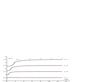
Figure 2: The Regge poles $\lambda_{n}(\omega)$ followed for $\omega=0\to 5$, $n=1,2,3,4$ for a scalar perturbation ($2M=1$).

Table 1: A sample of QNM frequencies for scalar perturbations ($2M=1$).

		Exact	Exact	Semiclassical	Semiclassical
$\ell$	$n$	$\omega^{(o)}_{\ell n}$	$\Gamma_{\ell n}/2$	$\omega^{(o)}_{\ell n}$	$\Gamma_{\ell n}/2$
0	1	0.22091	-0.20979	0.19009	-0.23120
	2	0.17223	-0.69610	0.09743	-0.33189
	3	0.15148	-1.20216	0.09695	-0.31452
1	1	0.58587	-0.19532	0.58336	-0.19653
	2	0.52890	-0.61252	0.51960	-0.59418
	3	0.45908	-1.08027	0.44000	-0.93961
2	1	0.96729	-0.19352	0.96669	-0.19371
	2	0.92716	-0.59121	0.92504	-0.58871
	3	0.86109	-1.01712	0.85890	-0.97714

He translates this requirement into an infinite-fraction equation involving the coefficients $\alpha$, $\beta$ and $\gamma$. Majumdar and Panchapakesan gave an alternative condition using the Hill determinant method Majumdar and Panchapakesan (1989): a set of parameters $\{l,\omega\}$ that give a convergent sum solve

$$D=\left|\begin{array}[]{ccccc}\beta_{0}&\alpha_{0}&\cdot&\cdot&\cdots\\ \gamma_{1}&\beta_{1}&\alpha_{1}&\cdot&\cdots\\ \cdot&\gamma_{2}&\beta_{2}&\alpha_{2}&\cdots\\ \vdots&\vdots&\ddots&\ddots&\ddots\\ \end{array}\right|=0.$$ (18)

This technique has the advantage of being more numerically tractable than Leaver’s, but it might be only valid for the Regge poles that lie close to the real axis of the CAM plane. Both Leaver’s original method and the Hill determinant method have been applied to the search for Regge poles in our study. We found excellent agreement between Leaver’s method and the Hill-determinant method for small values of Regge mode index $n$. We also agreed with Andersson’s values given in Ref. Andersson (1994). Fig. 2 exhibits the Regge trajectories numerically calculated while Table 1 presents a sample of QNM frequencies calculated from the semiclassical formulas (10) and (12). A comparison between the “exact” and the semiclassical spectra shows a good agreement, except for very low frequencies. Furthermore, the semiclassical theory permits us to classify the resonances in distinct families, each family being associated with one Regge pole and therefore to understand the meaning of the indices $n$ and $\ell$ introduced to denote the QNM frequencies $\omega_{\ell n}$.

At large $\omega$, the position of the Regge poles very closely adheres to the asymptotic form:

$$\lambda_{n}(\omega)\approx 3\sqrt{3}M\omega+i\left(n-1/2\right)\qquad n=1,2,3,\dots$$ (19)

Eq. (19) leads us to conclude that the $n$-th surface wave is localized near the unstable circular photon orbit at $R=3M$ by the following consistency argument: by reinstating dependence on Schwarzschild time $t$ into Eq. (II), we can see that the surface waves circle the black hole in time $T=2\pi\mathrm{Re}\ \lambda_{n}(\omega)/\omega\approx 2\pi 3\sqrt{3}M$ for large $\omega$. Furthermore, a photon on the circular orbit with constant radius $R$ takes the time $T^{\prime}=2\pi R/(1-2M/R)^{1/2}$ to circle the black hole (this result can be found by integrating the Schwarzschild metric $ds^{2}=0$). By equating $T$ and $T^{\prime}$, we obtain $R=3M$. Moreover, by using Eqs. (10), (12) and (19), we recover the well-known high-frequency behaviors (see Refs. Kokkotas and Schmidt, 1999 and Frolov and Novikov, 1998 and references therein)

$$\omega^{(o)}_{\ell n}\approx\frac{\ell+1/2}{3\sqrt{3}M}\quad\mathrm{and}\quad\frac{\Gamma_{\ell n}}{2}\approx\frac{n-1/2}{3\sqrt{3}M}.$$ (20)

These asymptotic behaviors have been obtained under the hypothesis $\mathrm{Re}\ \lambda_{n}(\omega)\gg\mathrm{Im}\ \lambda_{n}(\omega)$ and are therefore valid for $\ell\gg n$.

Our approach also applies to electromagnetic and gravitational scattering. In Fig. 3 and Table 2 we present some results for the latter case. A comparison between the exact and the semiclassical spectra shows a rather good agreement.

Finally, it seems to us necessary to emphasize that the CAM method we have developed here is based on two assumptions about the Regge poles $\lambda_{n}(\omega)$: They must formally satisfy $|\lambda_{n}(\omega)|\to+\infty$ as well as $\mathrm{Re}\ \lambda_{n}(\omega)\gg\mathrm{Im}\ \lambda_{n}(\omega)$ as $\omega\to\infty$. As a consequence, our method is a “high-frequency” approach which permits us to recover and to physically interpret the spectrum of the QNM frequencies lying in the region $2M\ \mathrm{Re}\ \omega>0.2$ of the complex $\omega$-plane. It should be noted that the highly damped QNM (for gravitational perturbations) as well as their associated frequencies which are connected with the area spectrum of the black hole (see Hod (1998) for the first paper on this subject and Baez (2003) and references therein for recent works in this domain) can neither be understood in the framework of our approach nor interpreted in terms of surface waves orbiting around the black hole near the unstable circular orbit at $r=3M$: Indeed, when the index $n$ is very large, the frequencies for these highly damped QNM are asymptotically given by Leaver (1985); Nollert (1993); Motl (gr-qc/0212096); Motl and Neitzke (hep-th/0301173)

$$\omega^{(o)}_{\ell n}\approx\frac{\ln 3}{8\pi M}\quad\mathrm{and}\quad\frac{\Gamma_{\ell n}}{2}\approx\frac{n+1/2}{4M}$$ (21)

and they therefore lie in the region $2M\ \mathrm{Re}\ \omega\ll 0.2$ and $2M\ |\mathrm{Im}\ \omega|\gg 1$ of the complex $\omega$-plane.

III Conclusion

To conclude, we would like first to comment on some aspects of our work and then to consider some possible extensions of the CAM approach in gravitational physics:

- We have established the connection between Andersson’s surface waves and the QNM complex frequencies of the Schwarzschild black hole in the particular context of wave scattering. This connection is more general and could be also obtained directly from the Regge-Wheeler equation, by extending the CAM method developed by Sommerfeld Sommerfeld (1949) as an alternative to the Watson approach Watson (1918).

- Because the gravitational radiation created in many black hole processes is dominated at intermediate timescales by QNMs, it can be always interpreted in terms of surface waves. Whatever the perturbation which modifies the geometry of a Schwarzschild black hole, it leads to the excitation of surface waves localized close to the unstable photon orbit. During its repeated circumnavigations, a given surface wave decays by radiating away its energy, leading to the damped ringing of the geometry. This mechanism is analogous to the damped ringing of the Earth which occurs during several days after a large earthquake and which can be explained in term of the Rayleigh surface wave.

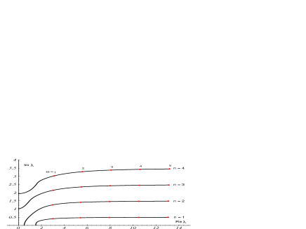
Figure 3: The Regge poles $\lambda_{n}(\omega)$ followed for $\omega=0\to 5$, $n=1,2,3,4$, for gravitational perturbations ($2M=1$).

Table 2: A sample of QNM frequencies for gravitational perturbations ($2M=1$).

		Exact	Exact	Semiclassical	Semiclassical
$\ell$	$n$	$\omega^{(o)}_{\ell n}$	$\Gamma_{\ell n}/2$	$\omega^{(o)}_{\ell n}$	$\Gamma_{\ell n}/2$
2	1	0.74734	-0.17793	0.75812	-0.17644
	2	0.69342	-0.54783	0.78134	-0.49976
	3	0.60211	-0.95655	0.77683	-0.83126
3	1	1.19889	-0.18541	1.20332	-0.18455
	2	1.16529	-0.56260	1.20089	-0.54409
	3	1.10337	-0.95819	1.18284	-0.89846
4	1	1.61836	-0.18832	1.62052	-0.18792
	2	1.59326	-0.56866	1.61119	-0.56020
	3	1.54542	-0.95982	1.58849	-0.92907

- The CAM method could be naturally introduced in many other areas of the physics of relativistic stars and black holes. Such a program could include in particular the following topics:

(i) The interpretation of the QNM of neutron stars and of the Kerr black hole in terms of surface waves. For the Kerr black hole, such an approach could easily explain the splitting of the quasinormal frequencies due to rotation.

(ii) The analysis of Hawking radiation as well as of Kerr black hole superradiance.

(iii) The study of black holes immersed in asymptotically anti-de Sitter space-times. The CAM approach could provide new tests of the AdS/CFT correspondence recently proposed in the context of superstring theory Maldacena (1998). With this aim in view, the (2+1)-dimensional BTZ black hole Banados et al. (1992) seems to us very interesting because, in that particular space-time, the wave equation can be solved exactly (see, e.g., Cardoso and Lemos (2001)) and therefore Regge poles can be analytically obtained.

(iv) The study of artificial black holes Novello et al. (2002). Here, it would be possible to benefit from the formidable CAM machinery developed in electromagnetism, optics and acoustics.