Global Monopole in General Relativity

Kirill A. Bronnikov† , Boris E. Meierovich and Evgeny R. Podolyak‡

†

Center for Gravitation and Fundamental Metrology, VNIIMS, 3-1 M. Ulyanovoy St., Moscow 117313, Russia;
Institute of Gravitation and Cosmology, PFUR, 6 Miklukho-Maklaya St., Moscow 117198, Russia

‡

P.L. Kapitza Institute of Physics Problems, 2 Kosygina St., Moscow 117334, Russia

1. Introduction

According to the Standard cosmological model [1], the Universe has been expanding and cooling from a split second after the Big Bang to the present moment and remained uniform and isotropic overall in doing so. In the process of its evolution, the Universe has experienced a chain of phase transitions with spontaneous symmetry breaking, including Grand Unification, electroweak phase transition, formation of neutrons and protons from quarks, recombination, and so forth. Regions with spontaneously broken symmetry, which are more than the correlation length apart, are statistically independent. At interfaces between these regions, so-called topological defects necessarily arise. A systematic exposition of the potential role of topological defects in our Universe is provided by Vilenkin and Shellard [2]. The particular types of defects: domain walls, strings, monopoles, or textures are determined by the topological properties of vacuum [5]. If the vacuum manifold after the breakdown is not shrinkable to a point, then the Polyakov-t’Hooft monopole-type solutions [3, 4] appear in quantum field theory.

Spontaneous symmetry breaking (SSB) plays a fundamental role in modern attempts to construct particle theories. A symmetry in this context is not necessarily associated with space-time transformations. It can be a kind of “internal” symmetry as well, such as the Grand Unification symmetry, the electroweak and the isotopic symmetry, or even supersymmetry, whose transformations mix bosons and fermions. Topological defects, caused by spontaneous breaking of internal symmetries (independent of space-time coordinates), are called global.

A fundamental property of global symmetry violation is the Goldstone degree of freedom. In the monopole case, the term related to the Goldstone boson in the energy-momentum tensor decreases rather slowly away from the center. As a result, the total energy of a global monopole grows linearly with distance, in other words, diverges. Without gravity such a divergence is a general property of spontaneously broken global symmetries. In his pioneering paper [3] Polyakov mentioned two possibilities of avoiding this difficulty. The first one was to combine a monopole with a Yang-Mills field. This idea was independently considered by t’Hooft [4]. This, among other reasons, gave rise to numerous papers on gauge (magnetic) monopoles. The second possibility was to consider a bound monopole-antimonopole system, whose total energy would be large (proportional to the distance between the components) but finite.

One more opportunity is to take into account the self-gravity of global monopoles, which can in principle remove the above self-energy problem. This is also necessary for potential astrophysical applications. Such a study was first performed by Barriola and Vilenkin [8] who found that the gravitational field outside a monopole is characterized by a solid angle deficit proportional to the SSB energy scale. Harari and Lousto showed that the gravitational mass of a global monopole, calculated using the Tolman integral, is negative [9]. Solutions with a horizon for supermassive global monopoles were found by Liebling [10], who also confirmed the estimate of Ref. [14] for the upper value of the symmetry breaking energy compatible with a static configuration. The existence of de Sitter cores inside global monopoles and other topological defects gave rise to the idea of “topological inflation” [11, 12, 13].

For global strings in flat space, the energy per unit length (without gravitation) also diverges with growing distance from the axis, but only logarithmically. However, in general relativity integration over the cross-section yields a finite result [6, 7]. The gravitational interaction thus leads to self-localization of a global string. Will a similar effect take place for a global monopole? An attempt to answer this question, which appears not to be answered in the existing papers, was one of motivations for reconsidering the gravitational properties of a global monopole.

The previous studies have used the boundary condition according to which the symmetry-breaking potential should vanish at spatial infinity. Our approach is different: we do not even assume the existence of a spatial asymptotic but require regularity at the center and try to observe the properties of the whole set of global monopole solutions. In doind so, among other quantities, we discuss the behavior of the total scalar field energy, which turns out to be finite in static regions of supermassive global monopoles.

In Sec. 2 we present the complete sets of equations for a static spherically symmetric gravitating global monopole in two most convenient coordinate systems, namely, with quasiglobal and harmonic radial coordinates. The general properties of static global monopoles are summarized in Sec. 3. In Sec. 4 we analyze analytically and numerically the specific features of a global monopole in the particular case of the “Mexican hat” potential. Sec. 5 contains a general discussion of our results, including their possible cosmological interpretation.

2. Equations and boundary conditions

2.1. General problem setting

We begin with the most general form of a static, spherically symmetric metric, without specifying the radial coordinate $x^{1}=u$:

$$ds^{2}=g_{\mu\nu}dx^{\mu}dx^{\nu}={\,\rm e}^{2F_{0}}dt^{2}-{\,\rm e}^{2F_{1}}du^{2}-{\,\rm e}^{2F_{\Omega}}d\Omega^{2}.$$ (1)

Here $d\Omega^{2}=d\theta^{2}+\sin^{2}\theta d\varphi^{2}$ is the linear element on a unit sphere and $F_{0}$, $F_{1}$, and $F_{\Omega}$ are functions of $u$.

The nonzero components of the Ricci tensor are (the prime denotes $d/du$)

$$R_{0}^{\ 0} = {\,\rm e}^{-2F_{1}}[F_{0}^{\prime\prime}+F_{0}^{\prime}(-F_{1}^{\prime}+2F^{\prime}_{\Omega}+F_{0}^{\prime})];$$

$${}R_{1}^{{\ }1} = {\,\rm e}^{-2F_{1}}[F_{0}^{\prime\prime}+2F^{\prime\prime}_{\Omega}+2F^{\prime}_{\Omega}{}^{2}+F^{\prime}_{0}{}^{2}-F_{1}^{\prime}(2F^{\prime}_{\Omega}+F^{\prime}_{0})];$$

$${}R_{2}^{\ 2} = R_{3}^{\ 3}=-{\,\rm e}^{-2F_{\Omega}}+{\,\rm e}^{-2F_{1}}[F^{\prime\prime}_{\Omega}+F^{\prime}_{\Omega}(-F_{1}^{\prime}+2F_{\Omega}^{\prime}+F_{0}^{\prime})].$$ (2)

Consider the Lagrangian describing a triplet of real scalar fields $\phi^{a}$ ($a=1,2,3$) in general relativity:

$$L=\frac{R}{16\pi G}+{{\displaystyle\frac{1}{2}}}g^{\mu\nu}\partial_{\mu}\phi^{a}\partial_{\nu}\phi^{a}-V(\phi),$$ (3)

where $R$ is the scalar curvature, $V(\phi)$ is a potential depending on $\phi=\pm\sqrt{\phi^{a}\phi^{a}}$ and $G$ is the gravitational constant. We use the natural units such that

$$\hbar=c=1,$$ (4)

so that $G=m_{\rm pl}^{-2}$, where $m_{\rm pl}=1.22\times 10^{19}$ GeV is the Planck mass.

To obtain a global monopole with unit topological charge [2], let us assume that the metric has the form (1) while $\phi^{a}$ comprise the following “hedgehog” configuration:

$$\phi^{a}=\phi(u)n^{a},\hskip 28.45274ptn^{a}=\left\{\sin\theta\cos\varphi,\quad\sin\theta\sin\varphi,\quad\cos\theta\right\}.$$ (5)

The Einstein equations can be written in the form

$$R_{\mu}^{\nu}=-8\pi G\tilde{T}_{\mu}^{\nu}=-8\pi G(T_{\mu}^{\nu}-{{\textstyle\frac{1}{2}}}\delta_{\mu}^{\nu}T^{\alpha}_{\alpha})$$ (6)

where $T_{\mu}^{\nu}$ is the energy-momentum tensor and the nonzero components of $\tilde{T}_{\mu}^{\nu}$ are

$$\tilde{T}_{0}^{0}=-V,\hskip 28.45274pt\tilde{T}_{1}^{1}=-V-{\,\rm e}^{-2F_{1}}\phi^{\prime}{}^{2},\hskip 28.45274pt\tilde{T}_{2}^{2}=\tilde{T}_{3}^{3}=-V-{\,\rm e}^{-2F_{\Omega}}\phi^{2}$$ (7)

The regular center conditions for the metric (1) are that at the corresponding value $u_{c}$ of the coordinate $x^{1}=u$

$${\,\rm e}^{F_{\Omega}}\to 0;\hskip 28.45274ptF_{0}=F_{0\,c}+O({\,\rm e}^{2F_{\Omega}}),\hskip 28.45274pt{\,\rm e}^{-F_{1}+F_{\Omega}}|F^{\prime}_{\Omega}|\to 1.$$ (8)

The last condition is necessary for local flatness and provides the correct circumference to radius ratio for coordinate circles at small $r={\,\rm e}^{F_{\Omega}}$.

The scalar field energy, defined as the partial time derivative of the scalar field action, $E=-\partial S/\partial t$, is a conserved quantity for our static system:

$$E=\int\sqrt{-g}T_{0}^{0}d^{3}x=4\pi\int{\,\rm e}^{F_{0}+F_{1}+2F_{\Omega}}\biggl{[}{{\displaystyle\frac{1}{2}}}{\,\rm e}^{-2F_{1}}\phi^{\prime}{}^{2}+{\,\rm e}^{-2F_{\Omega}}\phi^{2}+V\biggr{]}du,$$ (9)

where $g$ is the metric tensor determinant.

In what follows we will make some general inferences without specifying the potential $V(\phi)$ and then perform a more detailed study for the simplest and most frequently used symmetry-breaking potential

$$V(\phi)=\frac{1}{4}\lambda(\phi^{a}\phi^{a}-\eta^{2})^{2}=\frac{1}{4}\eta^{4}\lambda(f^{2}-1)^{2},$$ (10)

where $\eta>0$ characterizes the energy of symmetry breaking, $\lambda$ is a dimensionless constant and $f(u)=\phi(u)/\eta$ is the normalized field magnitude playing the role of an order parameter. The model has a global $SO(3)$ symmetry, which can be spontaneously broken to $SO(2)$ due to the potential wells ($V=0$) at $f=\pm 1$.

Let us now write down the Einstein equations and the boundary conditions explicitly in two coordinate frames to be used.

2.2. The quasiglobal coordinate $\rho$

The first choice is the coordinate $u=\rho$ specified by the condition $F_{0}+F_{1}=0$. Denoting ${\,\rm e}^{2F_{0}}={\,\rm e}^{-2F_{1}}=A(\rho)$ and ${\,\rm e}^{F_{\Omega}}=r(\rho)$, we obtain the metric in the form

$$ds^{2}=A(\rho)dt^{2}-\frac{d\rho^{2}}{A(\rho)}-r^{2}(\rho)d\Omega^{2}.$$ (11)

The scalar field equation

$$\mathop{\raisebox{3.5pt}{\large\framebox{}}}\nolimits\phi^{a}+\partial V/\partial\phi^{a}=0,$$ (12)

where $\mathop{\raisebox{3.5pt}{\large\framebox{}}}\nolimits=\nabla^{\alpha}\nabla_{\alpha}$ is the d’Alembert operator, and certain combinations of the Einstein equations have the form

$$(Ar^{2}\phi^{\prime})^{\prime}-2\phi = r^{2}dV/d\phi;$$ (13)

$$(A^{\prime}r^{2})^{\prime} = -16\pi Gr^{2}V;$$ (14)

$$2r^{\prime\prime}/r = -8\pi G\phi^{\prime}{}^{2};$$ (15)

$$A(r^{2})^{\prime\prime}-r^{2}A^{\prime\prime} = 2(1-8\pi G\phi^{2});$$ (16)

$$A^{\prime}rr^{\prime}+A{r^{\prime}}^{2}-1 = 8\pi G[{{\textstyle\frac{1}{2}}}Ar^{2}\phi^{\prime}{}^{2}-\phi^{2}-r^{2}V],$$ (17)

where the prime denotes $d/d\rho$. Only three of these five equations are independent: the scalar field equation (13) follows from the Einstein equations, while Eq. (17) is a first integral of the others. Given a potential $V(\varphi)$, this is a determined set of equations for the unknowns $r,\ A,\ \phi$.

This choice of the coordinates is preferable for considering Killing horizons, which correspond to zeros of the function $A(\rho)$, since such zeros are regular points of Eqs. (13)–(17); moreover, in a close neighborhood of a horizon, the coordinate $\rho$ defined in this manner varies (up to a positive constant factor) like manifestly well-behaved Kruskal-like coordinates used for analytic continuation of the metric [16, 17]. Therefore one can jointly consider regions at both sides of a horizon in terms of $\rho$, and, in general, the whole range of $\rho$ can contain several horizons. For this reason the coordinate $\rho$ can be called quasiglobal.

The regular center conditions (8) are fulfilled if, near some value $\rho_{c}$ of the coordinate $\rho$,

$$A(\rho)=A_{c}+O((\rho-\rho_{c})^{2}),\hskip 28.45274ptr(\rho)\approx(\rho-\rho_{c})/\sqrt{A_{c}}.$$ (18)

In regions where $A<0$ (sometimes called T-regions), if any, the coordinate $\rho$ is timelike and $t$ is space-like. Changing the notations, $t\to x\in{\mathbb{R}}$, and introducing the proper time of a comoving observer in a T-region,

$$\tau=\int d\rho/\sqrt{|A(\rho)|},$$ (19)

we can rewrite the metric in the form

$$ds^{2}=d\tau^{2}-|A(\tau)|dx^{2}-r^{2}(\tau)d\Omega^{2}.$$ (20)

The space-time geometry then corresponds to a homogeneous anisotropic cosmological model of Kantowski-Sachs (KS) type [23, 24], where spatial sections have the topology ${\mathbb{R}}\times{\mathbb{S}}^{2}$.

2.3. The harmonic coordinate $u$

Another convenient variable, well simplifying the form of the equations, is the harmonic coordinate $u$ specified by the condition [15]

$$F_{1}=2F_{\Omega}+F_{0},$$ (21)

so that $\mathop{\raisebox{3.5pt}{\large\framebox{}}}\nolimits u=0$. Then the field equations may be written as

$$\phi^{\prime\prime}-2{\,\rm e}^{F_{0}+F_{1}}\phi = {\,\rm e}^{2F_{1}}dV/d\phi,$$ (22)

$$F_{0}^{\prime\prime} = -8\pi G{\,\rm e}^{2F_{1}}V,$$ (23)

$$F_{1}^{\prime\prime}-2F_{\Omega}^{\prime}(F^{\prime}_{\Omega}+2F^{\prime}_{0}) = -8\pi G(\phi^{\prime}{}^{2}+{\,\rm e}^{2F_{1}}V),$$ (24)

$$F^{\prime\prime}_{\Omega}-{\,\rm e}^{2(F_{0}+F_{\Omega})} = -8\pi G(\phi^{2}{\,\rm e}^{2(F_{0}+F_{\Omega})}+{\,\rm e}^{2F_{1}}V),$$ (25)

$$-{\,\rm e}^{-2F_{\Omega}}+{\,\rm e}^{-2F_{1}}(F^{\prime}_{\Omega}{}^{2}+2F^{\prime}_{\Omega}F^{\prime}_{0}) = 8\pi G({{\textstyle\frac{1}{2}}}{\,\rm e}^{-2F_{1}}\phi^{\prime}{}^{2}-{\,\rm e}^{-2F_{\Omega}}\phi^{2}-V)$$ (26)

where the prime denotes $d/du$.

It is straightforward to obtain that a regular center can only correspond to $u\to\pm\infty$; we choose $u\to-\infty$, where one should have

$${\,\rm e}^{F_{\Omega}}\sim 1/|u|,\hskip 28.45274pt{\,\rm e}^{F_{0}}=\sqrt{A_{c}}(1+O(u^{-2})),\hskip 28.45274pt{\,\rm e}^{F_{1}}\sim 1/u^{2},$$ (27)

and $A_{c}$ is the same as in (18).

3. General properties of global monopoles

3.1. Monopoles in Minkowski space-time

The Minkowski metric in the usual spherical coordinates

$$ds^{2}=dt^{2}-dr^{2}-r^{2}d\Omega^{2}$$ (28)

is a special case of (11) with $r\equiv\rho$ and $A\equiv 1$. The only unknown in flat space-time is $\phi(r)$, and the only field equation is (13) which takes the form

$$(r^{2}\phi^{\prime})^{\prime}-2\phi=r^{2}dV/d\phi,$$ (29)

where, in particular, for the potential (10) $dV/d\phi=\lambda\phi(\phi^{2}-\eta^{2})$. In this case the scalar field equation can be written in terms of $f=\phi/\eta$ as

$$r^{-2}(r^{2}f^{\prime})^{\prime}-2fr^{-2}+\lambda\eta^{2}f(1-f^{2})=0.$$ (30)

The energy integral (9) takes the form

$$E=4\pi\int r^{2}\biggl{[}{{\displaystyle\frac{1}{2}}}\phi^{\prime}{}^{2}+\frac{\phi^{2}}{r^{2}}+V\biggr{]}dr,$$ (31)

and for its convergence, in case $V(\phi)\geq 0$, all the three terms should vanish quickly enough at infinity:

$$\phi=o(r^{-1/2}),\hskip 28.45274pt\phi^{\prime}=o(r^{-3/2}),\hskip 28.45274ptV=o(r^{-3})$$ (32)

as $r\to\infty$. This actually means that a configuration with finite energy is only possible with $V(0)=0$, contrary to the symmetry breaking assumption according to which $V$ has minima in nonsymmetric states, $\phi\neq 0$. In particular, the potential (10) does not give rise to global monopoles with finite energy. A consideration of self-gravity of the field triad $\phi^{a}$ is one of the ways to overcome this difficulty.

The harmonic coordinate $u$ in flat space-time is connected with $r$ by the relation $u-u_{0}=\pm 1/r$, where $u_{0}$ is an arbitrary constant; choosing the minus sign, we find that $u$ ranges from $-\infty$, which corresponds to the center $r=0$, to $u_{0}$ corresponding to spatial infinity.

3.2. Solutions with constant $\phi$

Under the assumption $\phi=\phi_{0}={\rm const}$, the corresponding value of the potential $V(\phi_{0})=V_{0}$ (times $8\pi G$) plays the role of a cosmological constant, and the Einstein equations can be integrated explicitly.

Indeed, in a region where $\phi={\rm const}$, Eq. (15) reduces to $r^{\prime\prime}=0$, whence $r=\alpha\rho+r_{0}$, $\alpha,\ r_{0}={\rm const}$. It remains to find $A(r)$, and this is immediately done by integrating Eq. (16):

$$A(r)=\frac{1-\Delta}{\alpha^{2}}-\frac{2GM}{r}+Cr^{2},\hskip 28.45274pt\Delta=8\pi G\phi_{0}^{2},$$ (33)

where $M$ and $C$ are integration constants. Substituting (33) into (14), we find

$$C=-8\pi GV_{0}/3.$$ (34)

Thus the solution is essentially determined by the values of $\phi_{0}$, $V_{0}$ and $M$. One more constant, $\alpha$, reflects the freedom in choosing the unit of time. It should be noted that this is not a monopole solution. Even if we put $M=0$, which is evidently necessary for regularity at $r=0$, this solution with constant $\phi\neq 0$ is singular at the center: for (33) with $M=0$ the Kretschmann scalar at small $r$ is ${\cal K}=R_{\alpha\beta\gamma\delta}R^{\alpha\beta\gamma\delta}\approx 4\Delta^{2}/r^{4}$.

With respect to a global monopole, two cases of the solution (33) are of interest. The case $\phi_{0}\equiv 0$ describes the symmetric state, while the case $V_{0}=0$ gives a possible asymptotic behavior at spatial or temporal infinity.

In case $\phi_{0}=0$ (the symmetric state), putting $M=0$ (which is necessary for a regular center), we arrive at the de Sitter metric

$$ds^{2}=\biggl{(}1-\frac{r^{2}}{r_{h}^{2}}\biggr{)}dt^{2}-\biggl{(}1-\frac{r^{2}}{r_{h}^{2}}\biggr{)}^{-1}dr^{2}-r^{2}d\Omega^{2},\hskip 28.45274ptr_{h}^{2}=\frac{8\pi GV_{0}}{3}.$$ (35)

This metric has a horizon at $r=r_{h}$. At $r>r_{h}$, outside the horizon, $r$ becomes a timelike coordinate, and $t$ is a spacelike one. Changing the notations as in (19), (20), we obtain the metric

$$ds^{2}=d\tau^{2}-\sinh^{2}(\tau/r_{h})dx^{2}-r_{h}^{2}\cosh^{2}(\tau/r_{h})d\Omega^{2}.$$ (36)

This is a KS cosmology with isotropic inflationary expansion at late times ($\tau\to\infty$).

In the other case, $\phi_{0}\neq 0$ but $V_{0}=0$ (the case of broken symmetry, such as $\phi=\eta$ in the potential (10)), the metric takes the form [8]

$$ds^{2}=\biggl{(}\frac{1-\Delta}{\alpha^{2}}-\frac{2GM}{r}\biggr{)}dt^{2}-\biggl{(}\frac{1-\Delta}{\alpha^{2}}-\frac{2GM}{r}\biggr{)}^{-1}dr^{2}-r^{2}d\Omega^{2},$$ (37)

where the constant $M$ has the meaning of mass in the sense that test particles at rest at large $r$ experience an acceleration equal to $-GM/r^{2}$ in the gravitational field (37). Furthermore, a nonzero value of $\phi_{0}$ leads to a solid angle deficit $\Delta$ defined in (33) at the asymptotic $r\to\infty$ (see [2] for more detail) and to a linear divergence of the integral (9) at large $r$.

The general case of Eq. (33) describes the large $r$ asymptotic of any solution to Eqs. (13)–(17), provided that such an asymptotic exists and $\phi$ tends quickly enough to a constant value.

For the monopoles to be studied, the metric (37) gives a large $r$ asymptotic in the case $\Delta<1$. We will also consider solutions with $\Delta>1$, for which a static asymptotic is absent. Then the metric (37) describes cosmological evolution at late times.

3.3. General properties of solutions with varying $\phi$

Consider now the general form of Eqs. (13)–(17) with varying $\phi$, without specifying the potential $V(\phi)$.

First of all, we note that, due to (15), $r^{\prime\prime}\leq 0$, which rules out any nonsingular configurations without a center such as wormholes and horns (see Theorem 1 of Ref. [17] for more detail).

Second, Eq. (16) can be rewritten in the form

$$(r^{4}B^{\prime})^{\prime}=-2(1-8\pi G\phi^{2}),\hskip 28.45274ptB\stackrel{{\scriptstyle\rm def}}{{=}}A/r^{2},$$ (38)

and at a point where $B^{\prime}=0$ we have $r^{4}B^{\prime\prime}=-2(1-8\pi G\phi^{2})$. Hence it follows that, as long as $\phi^{2}<1/(8\pi G)$ (the $\phi$ field does not reach trans-Planckian values), $B^{\prime\prime}<0$ at possible extrema of the function $B$. In other words, $B$ cannot have a regular minimum.

Our interest is in systems with a regular center satisfying the conditions (18), so that both $A(\rho)>0$ and $B(\rho)>0$ near $\rho=\rho_{c}$. At a possible horizon $\rho=h$, both $A$ and $B$ vanish, and, since it cannot be a minimum of $B$, $B<0$ at $\rho>h$ near the horizon. At greater $\rho$ the function $B(\rho)$, having no minima, can only decrease and will never return to zero; hence $A=Br^{2}<0$ at $\rho>h$. We conclude that there can be no more than one horizon, and, if it exists, it is simple (corresponds to a simple zero of $A(\rho)$). Since the global causal structure of space-time is determined (up to possible identifications of isometric hypersurfaces) by the number and disposition of Killing horizons [25, 26, 27], we have the following result:

Statement 1.  Under the assumption that $\phi^{2}<1/(8\pi G)$ in the whole space, our system with a regular center can have either no horizon, or one simple horizon, and in the latter case its global structure is the same as that of de Sitter space-time.

The above reasoning is in essence the same as in the proof of Theorem 2 of Ref. [17] on the disposition of horizons in scalar-vacuum space-times. It uses only Eq. (16) where the potential $V$ does not enter. Therefore the conclusion is valid for systems with any potentials, positive or negative.

Let us return to Eq. (15), according to which $r^{\prime\prime}\leq 0$. Since at a regular center $r^{\prime}>0$, this leaves three possibilities for the function $r(\rho)$ (see Fig. 1):

(a)

monotonic growth with a decreasing slope, but $r\to\infty$ as $\rho\to\infty$,

(b)

monotonic growth with $r\to r_{\max}<\infty$ as $\rho\to\infty$, and

(c)

growth up to $r_{\max}$ at some $\rho_{1}<\infty$ and further decrease, reaching $r=0$ at some finite $\rho_{2}>\rho_{1}$.

In each case, according to Statement 1, a horizon can occur at some $\rho=h$ within the range of $\rho$, so that at $\rho>h$ we have a T-region with the geometry of a KS cosmological model.

Figure 1: Possible behavior of $r(\rho)$ in global monopole solutions

We conclude that there are six classes of qualitative behaviors of the solutions, i.e., (a), (b), (c), each with or without a horizon, the latter circumstance to be labelled with the symbol 1 or 0, respectively. Thus, all solutions with a spatial asymptotic belong to class (a0). Class (b0) includes space-times ending with a “tube” consisting of two-dimensional spheres of equal radius. Class (c0) solutions contain a second center at $\rho=\rho_{2}$, and this center can a priori be regular or singular. We thus obtain a static analogue of closed cosmologies. Classes (a1), (b1), (c1) describe different late-time cosmological behaviors in the two directions corresponding to ${\mathbb{S}}^{2}$, whereas the fate of the third spatial direction (${\mathbb{R}}$) is determined by the function $A(\rho)$. In particular, the possible de Sitter asymptotic (36) belongs to class (a1) solutions, and in this case the expansion is isotropic at late times. On the other hand, class (c1) contains models which behave at late times like the Schwarzschild space-time inside the horizon, contracting to $r=0$.

This classification is obtained without any assumptions about $V(\phi)$. Solutions with given $V(\phi)$ will contain some of these classes, not necessarily all of them.

In case $V\geq 0$, Eq. (14) leads to one more important observation: since at a regular center $A^{\prime}r^{2}=0$, we can write (14) in the integral form

$$A^{\prime}r^{2}=-16\pi G\int_{0}^{\rho}V({\bar{\rho}})\,r^{2}({\bar{\rho}})\,d{\bar{\rho}}.$$ (39)

Thus, unless $V\equiv 0$, $A(\rho)$ is a decreasing function. Eq. (39) leads to the following conclusions.

Statement 1a.  If $V(\phi)\geq 0$, our system with a regular center can have either no horizon, or one simple horizon, and in the latter case its global structure is the same as that of de Sitter space-time.

Statement 2.  If $V(\phi)\geq 0$, the second center in class (c0) solutions is singular.

Statement 3.  If $V(\phi)\geq 0$ and the solution is asymptotically flat, the mass $M$ of the global monopole is negative.

Statement 1a shows that, for nonnegative potentials, the assumption $\phi^{2}<1/(8\pi G)$ in Statement 1 is unnecessary, and the causal structure types are known for any magnitudes of $\phi$.

Statement 2 follows from $A^{\prime}(\rho_{2})<0$, whereas at a regular center it should be $A^{\prime}=0$, see (18). $A^{\prime}(\rho_{2})=0$ could only be possible with $V\equiv 0$, but in this case the only solution with a regular center is trivial (flat space, $\phi=0$).

In Statement 3, asymptotic flatness is understood up to the solid angle deficit, i.e., $r=\rho$ and $A$ is given by (33) with $C=0$ at large $\rho$. Then, (39) for $\rho\to\infty$ gives $2GM$ on the left-hand side and a negative quantity on the right.

To our knowledge, this simple conclusion, valid for all nonnegative potentials, has been so far obtained only numerically for the particular potential (10) [9]. Note that Statement 3 is an extension to global monopoles of the so-called generalized Rosen theorem [22, 17], previously known for scalar-vacuum configurations.

Thus, even before studying particular solutions with the potential (10), we have a more or less complete knowledge of what can be expected from such global monopole systems.

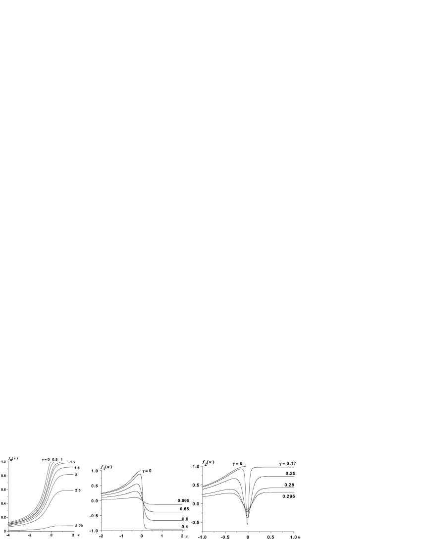
Figure 2: The field magnitude $f$ as a function of the harmonic coordinate $u$ for different values of $\gamma$. Solutions with monotonically growing $f=f_{0}(u)$ (a) exist for $0<\gamma<\gamma_{0}=3.$ In the region $\gamma<\gamma_{1}=2/3$ there are solutions with $f=f_{1}(u)$, changing their sign once (b), in the region $\gamma<\gamma_{2}=0.3$ there are solutions with $f=f_{2}(u)$ changing their sign twice (c). As $\gamma\to\gamma_{n}-0$, the function $f_{n}(u)$ vanishes in the whole range $-\infty<u<\infty$ from the center to the horizon.

4. Mexican hat potential

4.1. Equations and boundary conditions

Further analysis is performed for the particular “Mexican hat” potential (10). For numerical integration we prefer to use the harmonic coordinate $u$ and to work with Eqs. (22)–(25). This variable enters into the equations only via derivatives and is thus invariant under translations $u\to u+{\rm const}$.

Introducing the dimensionless quantities

$$\tilde{u}=u/(\sqrt{\lambda}\eta),\hskip 28.45274pt{\,\rm e}^{\tilde{F}_{\Omega}}=\sqrt{\lambda}\eta{\,\rm e}^{F_{\Omega}},\hskip 28.45274pt{\,\rm e}^{\tilde{F}_{1}}=\lambda\eta^{2}{\,\rm e}^{F_{1}}$$ (40)

we exclude the parameter $\lambda$ from the equations. Indeed, omitting the tildes, we obtain

$$f^{\prime\prime} = {\,\rm e}^{2(F_{0}+F_{\Omega})}[2-{\,\rm e}^{2F_{\Omega}}(1-f^{2})]f,$$ (41)

$$F^{\prime\prime}_{0} = -\frac{\gamma}{4}{\,\rm e}^{2(F_{0}+2F_{\Omega})}(f^{2}-1)^{2},$$ (42)

$$F^{\prime\prime}_{\Omega} = {\,\rm e}^{2(F_{0}+F_{\Omega})}[1-\gamma f^{2}-\frac{\gamma}{4}{\,\rm e}^{2F_{\Omega}}(1-f^{2})^{2}]$$ (43)

The condition (21) is preserved for the newly defined quantities, but the metric now reads

$$ds^{2}={\,\rm e}^{2F_{0}}dt^{2}-\frac{{\,\rm e}^{2F_{1}}du^{2}+{\,\rm e}^{2F_{\Omega}}d\Omega^{2}}{\lambda\eta^{2}}.$$ (44)

The boundary conditions at $u\to-\infty$ are

$$f=0,\qquad F_{0}=0,\qquad F^{\prime}_{0}=0,\qquad F_{\Omega}=-\ln(-u)+o(1/|u|),\qquad{\rm as}\quad u\to-\infty,$$ (45)

They follow from the requirement of regularity at the center and a particular choice of the time unit ($F_{0}=0$) and the origin of the $u$ coordinate (the fourth condition).

There remains only one dimensionless parameter in Eqs. (41)–(43),

$$\gamma=8\pi G\eta^{2},$$ (46)

it is the squared energy of symmetry breaking in Planck units.

It is easy to obtain that $\gamma=1$ is a critical value of this parameter. Indeed, if we suppose the existence of a large $r$ asymptotic at which $f\to 1$, i.e., the field tends to the minimum of the potential (10), then the asymptotic form of the metric at large $r$ is (37) with $\Delta=\gamma$. Consequently, the asymptotic can be static only if $\gamma\leq 1$, whereas for $\gamma>1$ the large $r$ asymptotic can be only cosmological (KS type), and there is a horizon separating such an outer region from the static monopole core.

On the other hand, if a configuration with $\gamma<1$ possesses a horizon, there is again a KS cosmology outside it, but there cannot be a large $r$ asymptotic and, according to Sec. 3, the solutions belong to classes (b1) or (c1).

Now, leaving aside the rather well studied case of solutions with a static asymptotic [2, 8, 9], belonging to class (a0) according to Sec. 3, let us suppose that there is a horizon and return to Eqs. (41)–(43). The horizon corresponds to $u\to+\infty$. For such cases, in addition to (45), we impose the boundary condition

$$f(u)\to f_{h},\hskip 28.45274pt|f_{h}|<\infty\hskip 28.45274pt{\rm as}\quad u\to+\infty.$$ (47)

This condition is necessary for regularity of a solution on the horizon and is applicable to classes (a1), (b1), (c1).

For class (a0) solutions, having a spatial asymptotic and no horizon, the condition (47) is meaningless. Moreover, the coordinate $u$ then ranges from $-\infty$ to some $u_{0}<\infty$ such that $r(u_{0})=\infty$.

For configurations of classes (a0) and (a1), the commonly used boundary condition at large $r$ is

$$f\to 1\hskip 28.45274pt{\rm as}\quad r\to\infty.$$ (48)

It is of interest that in the case (a1), to which both condition are applicable, the condition (47), being less restrictive, still leads to solutions satisfying (48) due to the properties of the physical system itself.

The set of equations (41)–(43) with the boundary conditions (45) and (47) comprise a well-posed nonlinear eigenvalue problem. Its trivial solution, with $f=0$ and the de Sitter metric (35), describes the symmetric state (with unbroken symmetry). Nontrivial solutions, describing hedgehog configurations with spontaneously broken symmetry, can be found numerically and yield a sequence of eigenvalues $\gamma_{n}$, $n=0,\ 1,\ \ldots$ and the corresponding values of the horizon radius $r_{h,n}$ for each given value of $f_{h}$. Conversely, for given (admissible) value of $\gamma$ one obtains a sequence of values of $f_{h}$ and $r_{h}$.

4.2. Linear eigenvalue problem

Liebling has found empirically the upper critical value $\gamma_{0}\approx 3$ for the existence of static solutions [10]. In this section we find a theoretical ground for this limit. Actually, we find analytically a sequence of critical values $\gamma_{n},$ $n=0,1,...$, such that for $\gamma<\gamma_{n}$ there exist static configurations with the field magnitude $f(u)$ changing its sign $n$ times.

Figure 3: $\gamma$ dependence of the values of $f(u)$ on the horizon, $f_{h,n}=f_{n}(u)\biggl{|}_{u\to\infty}$.

In the literature one can find only an analysis for $f(u)>0$. Our numerical integration of Eqs. (41)–(43) shows that, in addition to solutions with monotonically growing $f(u)$ (which exist for $\gamma<\gamma_{0}=3$, see Fig. 2a), for $\gamma<\gamma_{1}=2/3$  there are also regular solutions with $f(u)$ changing sign once, see Fig. 2b. For $\gamma<\gamma_{2}=0.3$ there are solutions with two zeros of $f(u)$ (Fig. 2c), etc. All these solutions have a horizon, and the absolute value of $f$ on the horizon $|f_{h,n}|=|f_{n}(\infty)|$ is a decreasing function of $\gamma$, vanishing as $\gamma\to\gamma_{n}-0$, see Fig. 3.

As $\gamma\to\gamma_{n}$, the function $f(u)$ vanishes in the whole range of $u$, and it is this circumstance that allows us to find the critical values $\gamma_{n}$ analytically. In a close neighborhood of $\gamma_{n}$ the field $f(u)$ within the horizon is small, $f^{2}\ll 1$, so that Eq. (41) reduces to a linear equation with given background functions $F_{0}$ and $F_{\Omega}$, corresponding to the de Sitter metric (35). In terms of the dimensionless spherical radius $r$, Eq. (41) takes the form

$$\frac{d}{dr}\biggl{[}r^{2}\biggl{(}1-\frac{r^{2}}{r_{h}^{2}}\biggr{)}\frac{df}{dr}\biggr{]}-(2-r^{2})f=0,$$ (49)

where $r_{h}=\sqrt{12/\gamma}$ is the value of $r$ on the horizon. The boundary conditions are

$$f\Big{|}_{r=0}=0,\hskip 28.45274pt|f(r_{h})|<\infty.$$ (50)

Nontrivial solutions of (49) with these boundary conditions exist for a sequence of eigenvalues $\gamma=\gamma_{n}$, $n=0,1,2,...,$ and the corresponding eigenfunctions $f_{n}(r)$, regular in the interval $0\leq r\leq r_{h}$, are simple polynomials:

$$f_{n}(r)=\sum_{k=0}^{n}a_{k}\biggl{(}\frac{r}{r_{h}}\biggr{)}^{2k+1}.$$ (51)

Substituting (51) into (49), we find the eigenvalues

$$r_{h,n}^{2}=2(2n+1)(n+2),\qquad\gamma_{n}=\frac{3}{(n+1/2)(n+2)},$$ (52)

and the recurrent relation

$$a_{k}=a_{k-1}\frac{(2k-1)(2k+2)-r_{h,n}^{2}}{(2k+1)(2k+2)-2},\qquad k=1,2,...,$$ (53)

allowing one to express all $a_{k},$ $k=1,2,...,n,$  in terms of $a_{0}$. Eq. (49) is linear and homogeneous, so $a_{0}$ is an arbitrary constant. For fixed $n$ the coefficients $a_{k}$ in (51) are

$$a_{k}=a_{0}\prod_{i=1}^{k}\frac{(2i-1)(2i+2)-r_{h,n}^{2}}{(2i+1)(2i+2)-2},\qquad n>0,\qquad 1\leq k\leq n.$$ (54)

The case

$$n=0,\qquad r_{h,0}=2,\qquad f_{0}(r)=a_{0}r/r_{h,0}$$

gives a monotonically growing function $f(u)$ in a close vicinity of $\gamma=\gamma_{0}=3$, see Fig. 2a. Thus the upper limit $\gamma_{0}=3$ for the existence of static monopole solutions, previously found numerically by Liebling [10], is now obtained analytically.

The case

$$n=1,\hskip 28.45274ptr_{h,1}=3\sqrt{2},\hskip 28.45274ptf_{1}(r)=a_{0}\frac{r}{r_{h,{1}}}\biggl{[}1-\frac{7}{5}\biggr{(}\frac{r}{r_{h,1}}\biggr{)}^{2}\biggr{]}$$

describes the function $f(u)$, changing its sign once, at $\gamma$ close to $\gamma_{1}=2/3$, see Fig. 2b. The case $n=2,$ $\gamma_{2}=3/10$, $r_{h,2}=2\sqrt{10}$,

$$f_{2}(r)=a_{0}\frac{r}{r_{h,{2}}}\biggl{[}1-\frac{18}{5}\biggl{(}\frac{r}{r_{h,{2}}}\biggr{)}^{2}+\frac{99}{35}\biggl{(}\frac{r}{r_{h,{2}}}\biggr{)}^{4}\biggr{]}$$

gives the field function $f(u)$ changing its sign twice (Fig. 2c).

For $n\gg 1$ the function $f_{n}(r)$ rapidly oscillates:

$$f_{n}(r)=a_{0}\frac{\cos\biggl{[}r_{h,n}\arcsin\sqrt{{\displaystyle\frac{r^{2}-2}{r_{h,n}^{2}-2}}}-\sqrt{2}\arcsin\biggl{(}{\displaystyle\frac{\sqrt{2}}{r}}\sqrt{{\displaystyle\frac{1-(r/r_{h,n})^{2}}{1-2/r_{h,n}^{2}}}}\biggl{)}\biggl{]}}{\sqrt[4]{r^{2}(r^{2}-2)\bigl{[}1-(r/r_{h,n})^{2}\bigr{]}}}.$$

However, this semiclassical formula is not valid near the left turning point $r=\sqrt{2}$, see dashed curve on Fig. 4. Its applicability range is $1\ll r<$ $r_{h,n}\approx 2n$, $n\gg 1$.

We have not met so far regular monopole configurations with the field function $f(u)$ changing its sign. It seems that this is their first presentation.

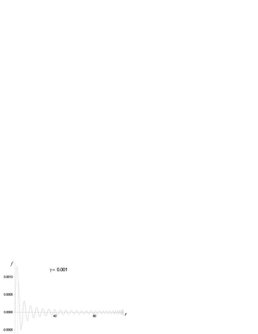
Figure 4: The field magnitude $f$ as a function of the spherical radius $r$ for $\gamma=0.001.$

4.3. Solutions with monotonically growing $f(u)$

As is clear from the aforesaid, the interval $0<\gamma<3$ of existence of nontrivial solutions with monotonically growing $f(u)$ splits into two qualitatively different regions, separated by $\gamma=1$.

In the interval $0<\gamma<1$ the solutions have the spatial asymptotic (37) and, according to our general classification, belong to class (a0). The spherical radius $r(u)={\,\rm e}^{F_{\Omega}(u)}$ varies from zero to infinity, $f(u)$ grows from zero to unity, $A(u)$ decreases from unity to its limiting positive value (compare with (37))

$$A\biggl{|}_{r\to\infty}=\frac{1-\gamma}{\alpha^{2}},\hskip 28.45274pt\alpha=\frac{dr}{d\rho}\biggl{|}_{\rho\to\infty}=1-\frac{\gamma}{2}\int_{0}^{\infty}f^{\prime}{}^{2}(\rho)r(\rho)d\rho,$$ (55)

and the energy integral (9) diverges.

In the interval $1<\gamma<3$, the solutions with monotonically growing $f(u)$ belong to class (a1). Instead of a spatial asymptotic, there is a horizon and a KS cosmology outside it. The functions $A$ and $r$ inside and outside the horizon are presented in Fig. 5 for $\gamma=2$.

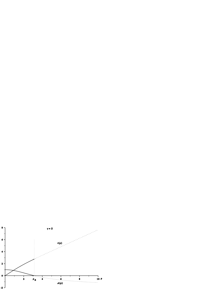
Figure 5: The functions $A(\rho)$ and $r(\rho)$ form unified smooth curves in the regions inside (solid curves) and outside (dotted) the horizon; $\gamma=2.$

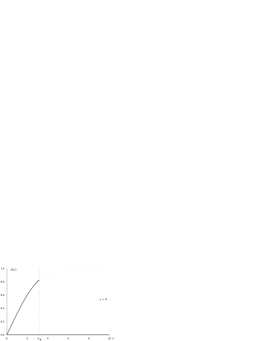
Figure 6: $f(\rho)$ inside (solid) and outside (dotted) the horizon; $\gamma=2$.

In the presence of a global monopole the cosmological expansion is slower than the de Sitter one (36). As $\tau\to\infty$, the radius $r(\tau)$ grows linearly, while $A$ tends to the negative constant value $-(\gamma-1)/\alpha^{2}$.

Within the horizon $f(u)$ monotonically grows from zero at $u=-\infty$ to a value $f_{h}=f_{h,0}(\gamma)$ on the horizon, $u\to\infty$, see Fig. 2a. The $f$ value on the horizon $f_{h,0}$ as a function of $\gamma$ decreases from unity at $\gamma=1$ to zero at $\gamma=\gamma_{0}=3$, see Fig. 3. The integral (9) taken over the static region converges, and we can conclude that at $1<\gamma<3$ the gravitational field is strong enough to suppress the Goldstone divergence and to localize the monopole. At $\gamma>3$ gravity is probably so strong that it restores the high symmetry of the system.

Outside the horizon the field $f$ as a function of the proper time $\tau$ grows from $f_{h,0}$ on the horizon to unity at $\tau\to\infty$. Introducing the proper radial length $l$ inside the horizon by the relation $dl=d\rho/\sqrt{A}$, one can ascertain that the functions $f(l(\rho))$ at $\rho<h$ and $f(\tau(\rho))$ at $\rho>h$ are two parts of a single smooth curve, see Fig. 6.

When the parameter $\gamma$ is close to its critical value ($\gamma=1$), separating the (a0) and (a1) branches of the solution, i.e., for

$$0<\gamma-1\ll 1.$$ (56)

one can find analytically the horizon radius $r_{h,0}$ and the scalar field value on the horizon $f_{h,0}$ under certain additional assumptions on the system behavior which follow from the results of numerical analysis. In particular, there is an “intermediate” region of the $u$ range, $1\ll u\ll u_{0}={\rm const}$, where the first term $f^{\prime\prime}$ in the scalar field equation (41) is very small whereas the function ${\,\rm e}^{2(F_{0}+F_{\Omega})}$ is quite large (despite the fact that this function eventually vanishes as $u\to\infty$). Therefore in this region the expression in square brackets should be small, i.e.,

$${\,\rm e}^{2F_{\Omega}}(1-f^{2})\approx 2,$$

and this relation can be used for further estimates.

The results are

$${}\ln r_{h,0}\approx\ln[1/(\gamma-1)]\gg 1,\hskip 28.45274ptf_{h,0}\approx 1-C(\gamma-1)^{2},$$ (57)

where the constant $C$ can be found by comparison with the numerical results; our estimate is $C\approx 0.3$

The solution behavior in the critical regime, $\gamma=1$, can be characterized as a globally static model with a “horizon at infinity” [10] since $A\to 0$ as $r\to\infty$.

The fact that monotonic solutions with horizons are absent for $\gamma<1$ becomes clear from an analysis of the inflection point $u=u_{\rm inf}$ of the function $F_{\Omega}(u)$. A horizon, if any, corresponds to $u\to\infty$ where $F_{\Omega}$ remains finite. Since it behaves logarithmically as $u\to-\infty$, there is (at least one) inflection point, where the second-order derivative is zero, and from Eq. (43) we have

$$1-\gamma f^{2}-\frac{\gamma}{4}{\,\rm e}^{2F_{\Omega}}(f^{2}-1)^{2}=0,\hskip 28.45274ptu=u_{\rm inf}.$$

This is a quadratic equation with respect to $1-f^{2}$, whence

$$1-f^{2}=2{\,\rm e}^{-2F_{\Omega}}\biggl{(}1\pm\sqrt{1-\frac{\gamma-1}{\gamma}{\,\rm e}^{2F_{\Omega}}}\biggr{)}.$$ (58)

A monotonically growing function $f(u)$ corresponds to greater values of $f$, i.e., to the “minus” branch of (58) (as is confirmed by numerical results). But then the r.h.s. of (58) is negative for $\gamma<1$, leading to $f^{2}>1$, which cannot happen since $f^{2}=1$ is the maximum attainable value for the solutions under study. Thus, for $\gamma<1$, all solutions with monotonically growing $f(u)$ belong to class (a0), possess a spatial asymptotic with a solid angle deficit and a divergent field energy.

Numerical integration confirms these conclusions. The different behavior of $F_{\Omega}(u)$ for $\gamma<1$ and $\gamma>1$ is shown in Fig. 7.

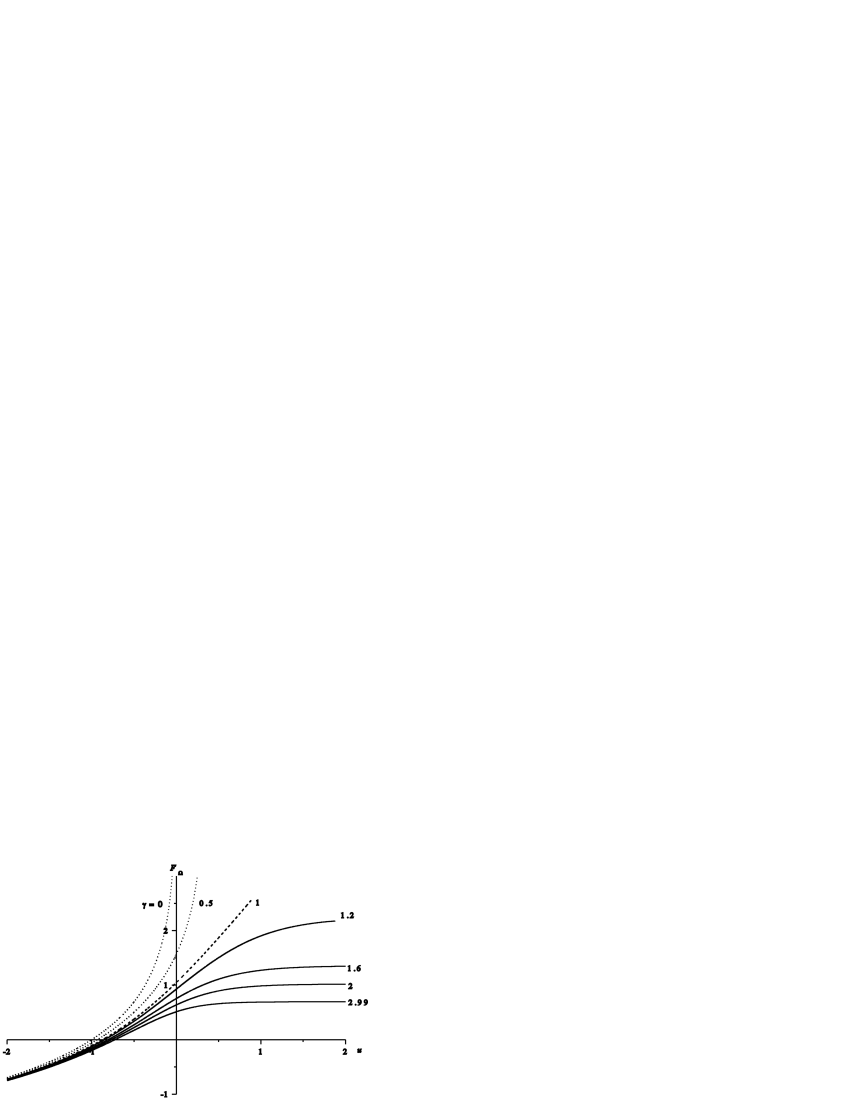
Figure 7: The function $F_{\Omega}(u)$ for different values of $\gamma$. At $\gamma<1$ there is a limiting value $u_{\max}$ of $u$, such that $F_{\Omega}\to\infty$ as $u\to u_{\max}(\gamma)$ (dotted curves). As $\gamma\to 1$, the value $u_{\max}(\gamma)\to\infty$ (dashed curve), and, for $\gamma>1$, $F_{\Omega}(u)$ tends to a finite constant value as $u\to\infty$ (solid curves).

4.4. Solutions with $f(u)$ changing its sign

For $\gamma<\gamma_{1}=2/3$ there are solutions with the function $f(\phi)$ changing its sign once, see Fig. 2b. For $\gamma<\gamma_{2}=0.3$ there are solutions where $f(\phi)$ changes its sign twice, see Fig. 2c, etc. Unlike the monotonic solutions discussed in Sec. 4.3, all of them possess a horizon, and, in agreement with the general inferences of Sec. 4.1, they belong to class (c1). This means that, beginning with a regular center, the spherical radius $r(\rho)$ first grows, then passes its maximum $r_{\max}$ at some $\rho_{1}$ and then decreases to zero at finite $\rho=\rho_{2}$ which is a singularity. The horizon occurs at some $\rho=h<\rho_{2}$, which can be greater or smaller than $\rho_{1}$, but in any case the singularity takes place in a T-region and is of cosmological nature. The dependence $r(\rho)$ before and after the horizon is a single smooth curve, see Fig. 8a.

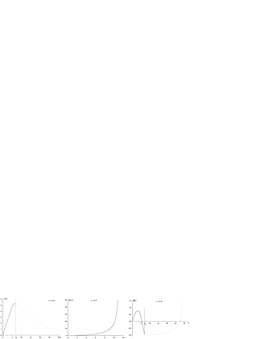
Figure 8: Solutions with $f$ of alternating sign: the functions (a) $r(\rho),$ (b) $|A(\rho)|,$ and (c) $f(\rho)$ for $\gamma=0.5$ before (solid) and after (dotted) the horizon.

Beyond the horizon, $|A(\tau)|$ as a function of the proper time $\tau$ of a comoving observer grows from zero at $\tau=0$ (the horizon) to infinity at $\tau\to\tau_{s}=\tau(\rho_{2})$ (the singularity), see Fig. 8b. The scalar field magnitude $|f(\tau)|$ beyond the horizon first grows, then slightly varies around unity. Approaching the singularity, $f(\tau)$ changes its sign and finally $|f(\tau)|\to\infty$ as $\tau\to\tau_{s}$, see Fig. 8c.

5. Conclusion and discussion

We have performed a general study of the properties of static global monopoles in general relativity. We have shown that, independently of the shape of the symmetry breaking potential, the metric can contain either no horizon, or one simple horizon, and in the latter case the space-time global structure is the same as that of de Sitter space-time. Outside the horizon the geometry corresponds to homogeneous anisotropic cosmological models of KS type, where spatial sections have the topology ${\mathbb{R}}\times{\mathbb{S}}^{2}$. In general, all possible solutions can be divided into six classes with different qualitative behavior. This classification is obtained without any assumptions about $V(\phi)$. Solutions with given $V(\phi)$ contain some of these classes, not necessarily all of them. This qualitative analysis gives a complete picture of what can be expected for global monopole systems with particular symmetry breaking potentials.

Our analytical and numerical analysis for the particular case of “Mexican hat” potential confirmed the previous results of other authors concerning the configurations with monotonically growing order parameter. Among other things, we have obtained analytically the upper limit $\gamma_{0}=3$ for the existence of static monopole solutions, previously found numerically by Liebling [10]. We have also found and analyzed a new family of solutions with the field function $f$ changing its sign, which we have not met in the existing literature.

Of particular interest can be the class (a1) solutions with a static nonsingular monopole core and a KS cosmological model outside the horizon. Its anisotropic evolution is determined by the functions of the proper time $|A(\tau)|$ (the squared scale factor in the ${\mathbb{R}}$ direction, $r(\tau)$ (the scale factor in the two ${\mathbb{S}}^{2}$ directions) and the field magnitude $f(\tau)$. For a comoving observer in the T-region, the expansion starts with a rapid growth of $|A(\tau)|$ from zero to finite values, resembling inflation, and ending with $A\to{\rm const}$ as $\tau\to\infty$. The expansion in the ${\mathbb{S}}^{2}$ directions, described by $r(\tau)$, is comparatively uniform and linear at late times, i.e., much slower than the de Sitter’s $\cosh^{2}(\tau/r_{h})$, see (35). It should be stressed that all such models with de Sitter-like causal structure, i.e., a static core and expansion beyond a horizon, drastically differ from standard Big Bang models in that the expansion starts from a nonsingular surface, and cosmological comoving observers can receive information in the form of particles and light quanta from the static region, situated in the absolute past with respect to them. Moreover, in our case the static core is nonsingular, and it is thus an example of an entirely nonsingular cosmology in the spirit of papers by Gliner and Dymnikova [28, 29].

The nonzero symmetry-breaking potential plays the role of a time-dependent cosmological constant, a kind of hidden vacuum matter. Since the field function $f$ tends to unity as $\tau\to\infty$, the potential vanishes, and the “hidden vacuum matter” disappears.

The lack of isotropization at late times does not seem to be a fatal shortcoming of the model for two reasons. First, if the model is applied for describing the near-Planck epoch of the Universe evolution, then, on the next stage, the anisotropy can probably be damped by diverse particle creation, and the further stages with lower energy densities may conform to the standard picture (with possible further phase transitions). Second, if we add a comparatively small positive quantity $\Lambda$ to the potential (10) (“slightly raise the Mexican hat”), this must change nothing but the late-time asymptotic which will become de Sitter, corresponding to the cosmological constant $\Lambda$. In our view, these ideas deserve a further study.

Evidently, the present simple model cannot be directly applied to our Universe. It would be too naive to expect that a macroscopic description based on a simple toy model of a global monopole with only one dimensionless parameter $\gamma$ can explain the whole variety of early-Universe phenomena. Nevertheless, it may be considered as an argument in favor of the idea that the standard Big Bang might be replaced with a nonsingular static core and a horizon appearing as a result of some symmetry-breaking phase transition on the Planck energy scale.

6. Acknowledgement

The authors are grateful to Acad. A.F. Andreev for a useful discussion at the seminar at P.L. Kapitza Institute of Physical Problems.

References

- [1] Ya.B. Zel’dovich and I.D. Novikov, “Relativistic Astrophysics”, Moscow, Nauka, 1967.
- [2] A. Vilenkin and E.P.S. Shellard, “Cosmic Strings and other Topological Defects”, Cambridge University Press, Cambridge, 1994.
- [3] A.M. Polyakov, Zh. Eksp. Teor. Fiz. 20, 430 (1974) [JETP Lett. 20, 194 (1974) ].
- [4] G. ’t Hooft, Nucl. Phys. B79, 276 (1974).
- [5] T.W.B. Kibble. J. Phys. A9, 1387 (1976).
- [6] B.E. Meierovich, Gen. Rel. Grav. 33, 405 (2001).
- [7] B.E. Meierovich and E.R. Podolyak, Grav. & Cosmol. 7, 117 (2001).
- [8] M. Barriola and A. Vilenkin, Phys. Rev. Lett. 63, 341 (1989).
- [9] D. Harari and C. Lousto, Phys. Rev. D 42, 2626 (1990).
- [10] S.L. Liebling, Phys. Rev. D 61, 024030 (1999).
- [11] A. Vilenkin, Phys. Rev. Lett. 72, 3137 (1994).
- [12] A. Linde, Phys. Lett. 327B, 208 (1994).
- [13] R. Basu and A. Vilenkin, Phys. Rev. D 50, 7150 (1994).
- [14] N. Sakai, H. Shinkai, T. Tachizawa, K. Maeda, Phys. Rev. D 53, 655 (1996).
- [15] K.A. Bronnikov, Acta Phys. Polon. B 4, 251 (1973).
- [16] K.A. Bronnikov, G. Clément, C.P. Constantinidis and J.C. Fabris, Phys. Lett. 243A, 121 (1998), gr-qc/9801050; Grav. & Cosmol. 4, 128 (1998), gr-qc/9804064.
- [17] K.A. Bronnikov, Phys. Rev. D 64, 064013 (2001).
-
[18]
B. E. Meierovich,
Zh. Eksp. Teor. Fiz. 112, 385 (1997)
[Sov. Phys. JETP 85, 209 (1997)];
Grav. & Cosmol. 3, 29 (1997); Phys. Rev. D61, 024004, (2000). - [19] B. E. Meierovich and E. R. Podolyak, Phys. Rev. D 61, 125007 (2000).
- [20] B. E. Meierovich, Physics — Uspekhi 44, 981 (2001).
- [21] L. D. Landau and E. M. Lifshitz, “Quantum mechanics”, Nauka, Moscow, 1974.
- [22] K.A. Bronnikov and G.N. Shikin, “Self-gravitating particle models with classical fields and their stability”. Series “Itogi Nauki i Tekhniki” (“Results of Science and Engineering”), Subseries “Classical Field Theory and Gravitation Theory”, v. 2, p. 4, VINITI, Moscow 1991 (in Russian).
- [23] A.S. Kompaneets and A.S. Chernov, Zh. Eksp. Teor. Fiz. 47, 1939 (1964); Sov. Phys. JETP 20, 1303 (1965).
- [24] R. Kantowski and R.K. Sachs, J. Math. Phys. 7 443, (1966).
- [25] K.A. Bronnikov, Izv. Vuzov, Fizika, 1979, No. 6, 32-38.
- [26] M.O. Katanaev, Nucl. Phys. Proc. Suppl. 88, 233–236 (2000), gr-qc/9912039; Proc. Steklov Inst. Math. 228, 158–183, gr-qc/9907088.
- [27] T. Klosch and T. Strobl, Clas. Qu. Grav. 13, 1395–2422 (1996); 14, 1689–1723 (1997).
- [28] E.B. Gliner, Uspekhi Fiz. Nauk 172, No.2, 221 (2002).
- [29] E.B. Gliner and I.G. Dymnikova, Pis’ma v Astron. Zh. 1 (5), 7 (1975); reprinted in Uspekhi Fiz. Nauk 172, No.2, 227 (2002).