Late-time asymptotic dynamics of Bianchi VIII cosmologies

Abstract

In this paper we give, for the first time, a complete description of the late-time evolution of non-tilted spatially homogeneous cosmologies of Bianchi type VIII. The source is assumed to be a perfect fluid with equation of state $p=(\gamma-1)\mu$, where $\gamma$ is a constant which satisfies $1\leqslant\gamma\leqslant 2$. Using the orthonormal frame formalism and Hubble-normalized variables, we rigorously establish the limiting behaviour of the models at late times, and give asymptotic expansions for the key physical variables.

The main result is that asymptotic self-similarity breaking occurs, and is accompanied by the phenomenon of Weyl curvature dominance, characterized by the divergence of the Hubble-normalized Weyl curvature at late times.

1 Introduction

A long term goal in theoretical cosmology is to understand the structure and properties of the space of all cosmological solutions of the Einstein field equations (EFEs), with a view to shedding light on the evolution of the physical universe from the Planck time onward. In particular one wants to study deviations from the familiar Friedmann-Lemaître (FL) models, which describe a universe that is exactly homogeneous and isotropic on a suitably large scale. In working towards this goal one makes use of a symmetry-based hierarchy of cosmological models of increasing complexity, starting with the familiar FL models:

1. FL cosmologies

2. non-tilted spatially homogeneous (SH) cosmologies

3. tilted SH cosmologies

4. $G_{2}$ cosmologies

5. $G_{1}$ cosmologies

6. generic cosmologies

The terminology used in this hierarchy has the following meaning. A SH cosmology is said to be tilted if the fluid velocity vector is not orthogonal to the group orbits, otherwise the model is said to be non-tilted. A $G_{2}$ cosmology admits a local two-parameter Abelian group of isometries with spacelike orbits, permitting one degree of freedom as regards spatial inhomogeneity, while a $G_{1}$ cosmology admits one spacelike Killing vector field.

An important mathematical link between the various classes in the hierarchy is provided by the idea of representing the physical state of a cosmological model at an instant of time by a point in a state space, which is finite dimensional for classes i)–iii) and infinite dimensional otherwise. The EFEs are formulated as first order evolution equations, and the evolution of a cosmological model is represented by an orbit (i.e. a solution curve) of the evolution equations in the state space. The state space of a particular class in the hierarchy is a subset of the state spaces of the more general classes, which implies that the particular models are represented as special cases of the more general models. This structure opens the possibility that the evolution of a model in one class may be approximated, over some time interval, by a model in a more special class.

Detailed information about the evolution of cosmological models more general than FL models can only be obtained using numerical simulations or perturbation theory. On the other hand, by introducing suitably normalized variables, one can hope to use methods from the theory of dynamical systems to obtain qualitative information about the asymptotic regimes of cosmological models, namely

1. the approach to the initial singularity, characterized by $\ell\rightarrow 0^{+}$, and

2. the late-time evolution, characterized by $\ell\rightarrow+\infty$,

where $\ell$ is the overall length scale. From a dynamical systems point of view, the evolution in the asymptotic regimes is governed by the dynamics on the past attractor and the future attractor, respectively. From a physical point of view the asymptotic regime $\ell\rightarrow 0^{+}$ corresponds to the approach to the Planck time, while the asymptotic regime $\ell\rightarrow+\infty$ could describe the later stages of a particular epoch in the evolution of the universe, for example the radiation-dominated epoch in the early universe.

The above comments provide the background for the present paper, which deals with one of the unsolved problems concerning non-tilted SH cosmologies. There are two generic classes of non-tilted ever-expanding SH cosmologies, namely Bianchi type VIII and exceptional Bianchi type VI${}_{-1/9}^{\ast}$, neither of which have been fully analyzed. In this paper our interest lies in the late-time asymptotic regime of Bianchi VIII models. Two important results concerning this regime have been proved. Firstly, a theorem of Wald (1983) shows that Bianchi VIII models with a cosmological constant are asymptotic at late times to the de Sitter model, subject to rather weak restrictions on the stress-energy tensor. Secondly, Ringström (2001) has recently determined rigorously the late-time behaviour of vacuum Bianchi VIII models. We will comment on his results later. On the other hand, little is known about non-vacuum models with zero cosmological constant, apart from a brief heuristic discussion of models containing dust or radiation by Doroshkevich et al(1973) and by Lukash (1974). We likewise comment on these results later. In the present paper we give a rigorous analysis of the asymptotic dynamics at late times of Bianchi VIII cosmologies whose matter content is a perfect fluid with equation of state $p=(\gamma-1)\mu$, where $\gamma$ is a constant. This equation of state includes the physically important cases of dust ($\gamma=1$) and radiation ($\gamma=\frac{4}{3}$).

To achieve our goal we formulate the EFEs for the Bianchi VIII cosmologies as an asymptotically autonomous system of ordinary differential equations, using the Hubble-normalized variables first introduced by Wainwright and Hsu (1989) and modified by Wainwright et al(1999) and Nilsson et al(2000) in their study of the more special Bianchi VII₀ models. We are then able to apply a theorem of Strauss and Yorke (1967) concerning the solutions of asymptotically autonomous systems of differential equations.

The paper is organized as follows. In section 2 we present the evolution equations for SH cosmologies of Bianchi type VIII using the orthonormal frame formalism and Hubble-normalized variables. The equations are derived in detail in Wainwright and Ellis (1997) (see chapters 5 and 6). A change of variable then leads to a new form of the evolution equations that is adapted to the oscillatory nature of the Bianchi VIII models. In section 3 we present the main results, namely theorem 3.5 and corollary 3.1, which give the limits in the late-time regime of the expansion-normalized variables and of certain physical dimensionless scalars, thereby describing the asymptotic dynamics. In section 4 we strengthen the results of the theorem and corollary by giving the asymptotic form of the expansion-normalized variables and physical scalars at late times. The notions of asymptotic self-similarity breaking and Weyl curvature dominance are discussed in section 5. Finally, in section 6 we conclude by giving an overview of the asymptotic dynamics of non-tilted SH perfect fluid cosmologies, noting that the present paper and the accompanying paper Hewitt et al(2002) fill the gaps that exist in the literature.

There are four appendices. Appendix A contains the proof of the fact that Bianchi VIII universes are not asymptotically self-similar at late times. Appendix B contains the proof of theorem 3.5 while in appendix C we provide an outline of the derivation of the asymptotic forms at late times. Finally, in appendix D we give expressions for the components of the Weyl curvature tensor in terms of the expansion-normalized variables.

2 Evolution equations

In this section we give the evolution equations for non-tilted SH cosmologies of Bianchi type VIII. As described in WE (see pp 124–5), we use expansion-normalized variables

$$(\Sigma_{+},\Sigma_{-},N_{1},N_{2},N_{3}),$$ (2.1)

defined relative to a group-invariant orthonormal frame $\{\boldsymbol{e}_{a}\}$, with $\boldsymbol{e}_{0}=\boldsymbol{u}$, the fluid 4-velocity, which is normal to the group orbits.

The variables $\Sigma_{\pm}$ describe the shear of the fluid congruence, and the $N_{\alpha}$, $\alpha=1,2,3$ describe the intrinsic curvature of the group orbits. The models of Bianchi type VIII are described by the inequality $N_{1}N_{2}N_{3}<0$. Without loss of generality, we assume

$$N_{1}<0,\qquad N_{2}>0,\qquad N_{3}>0.$$ (2.2)

It is convenient to define

$$N_{+}={\textstyle\frac{1}{2}}(N_{2}+N_{3}),\qquad N_{-}={\textstyle\frac{1}{2\sqrt{3}}}(N_{2}-N_{3}),$$ (2.3)

and replace (2.1) by the state vector

$$(\Sigma_{+},\Sigma_{-},N_{1},N_{+},N_{-}).$$ (2.4)

The restrictions (2.2) become

$$N_{1}<0,\qquad N_{+}^{2}-3N_{-}^{2}>0,\qquad N_{+}>0.$$ (2.5)

The state variables (2.1) and (2.4) are dimensionless, having been normalized with the Hubble scalar $H$, which is related to the overall length scale $\ell$ by

$$H=\frac{\dot{\ell}}{\ell},$$ (2.6)

where the overdot denotes differentiation with respect to clock time along the fluid congruence. The state variables depend on a dimensionless time variable $\tau$ that is related to the length scale $\ell$ by

$$\ell=\ell_{0}\rme^{\tau},$$ (2.7)

where $\ell_{0}$ is a constant. The dimensionless time $\tau$ is related to the clock time $t$ by

$$\frac{\rmd t}{\rmd\tau}=\frac{1}{H},$$ (2.8)

as follows from equations (2.6) and (2.7). In formulating the evolution equations we require the deceleration parameter $q$, defined by

$$q=-\frac{\ell\ddot{\ell}}{\dot{\ell}^{2}},$$ (2.9)

and the density parameter $\Omega$, defined by

$$\Omega=\frac{\mu}{3H^{2}}.$$ (2.10)

In terms of the variables (2.4), the evolution equations (6.9) and (6.10) in WE become

$$\eqalign{\Sigma^{\prime}_{+}&=-(2-q)\Sigma_{+}-2N_{-}^{2}+{\textstyle\frac{1}{3}}N_{1}(N_{1}-N_{+}),\\ \Sigma^{\prime}_{-}&=-(2-q)\Sigma_{-}-N_{-}(2N_{+}-N_{1}),\\ N^{\prime}_{1}&=(q-4\Sigma_{+})N_{1},\\ N^{\prime}_{+}&=(q+2\Sigma_{+})N_{+}+6\Sigma_{-}N_{-},\\ N^{\prime}_{-}&=(q+2\Sigma_{+})N_{-}+2\Sigma_{-}N_{+},}$$ (2.16)

where

$$q =2(\Sigma_{+}^{2}+\Sigma_{-}^{2})+{\textstyle\frac{1}{2}}(3\gamma-2)\Omega,$$ (2.17)

$$\Omega =1-\Sigma_{+}^{2}-\Sigma_{-}^{2}-N_{-}^{2}-{\textstyle\frac{1}{12}}N_{1}^{2}-\left(-{\textstyle\frac{1}{3}}N_{1}N_{+}\right),$$ (2.18)

and ^′ denotes differentiation with respect to $\tau$. For future reference we also note the evolution equation for $\Omega$:

$$\Omega^{\prime}=[2q-(3\gamma-2)]\Omega.$$ (2.19)

The physical requirement $\Omega\geqslant 0$, in conjunction with (2.5), implies that the variables $\Sigma_{+}$, $\Sigma_{-}$, $N_{-}$, $N_{1}$ and $N_{1}N_{+}$ are bounded, but places no restriction on $N_{+}$ itself. In fact, it will be shown in appendix A (see proposition 1.1) that if $\Omega\geqslant 0$ and $\frac{2}{3}\leqslant\gamma\leqslant 2$, then for any initial conditions

$$\lim_{\tau\rightarrow+\infty}N_{+}=+\infty.$$ (2.20)

Inspection of the equations for $\Sigma^{\prime}_{+}$ and $N^{\prime}_{-}$ shows that this unboundedness of $N_{+}$ will induce rapid oscillations in $\Sigma_{-}$ and $N_{-}$ at late times, which further complicates the dynamics. A similar situation occurs in the Bianchi VII₀ models analyzed in WHU (see p 2583). The first step in analyzing the dynamics at late times ($\tau\rightarrow+\infty$) is to introduce new variables which are bounded at late times and which enable us to isolate the oscillatory behaviour associated with $\Sigma_{-}$ and $N_{-}$. We define

$$\eqalign{\Sigma_{-}=R\cos\psi,&\qquad N_{-}=R\sin\psi,\\ M=\frac{1}{N_{+}},&\qquad Z^{2}=-\frac{1}{3}N_{1}N_{+},}$$ (2.23)

where $R\geqslant 0$.

In terms of the new variables $(\Sigma_{+},R,Z,M,\psi)$, the evolution equations (2.16) can be shown to have the following form

$$\eqalign{\Sigma^{\prime}_{+}&=-(2-Q)\Sigma_{+}-R^{2}+Z^{2}+3M^{2}Z^{4}+(1+\Sigma_{+})R^{2}\cos 2\psi,\\ R^{\prime}&=\left[(Q+\Sigma_{+}-1)+(R^{2}-1-\Sigma_{+})\cos 2\psi-{\textstyle\frac{3}{2}}MZ^{2}\sin 2\psi\right]R,\\ Z^{\prime}&=\left[Q-\Sigma_{+}+R^{2}\left(\cos 2\psi+{\textstyle\frac{3}{2}}M\sin 2\psi\right)\right]Z,\\ M^{\prime}&=-\left[Q+2\Sigma_{+}+R^{2}\left(\cos 2\psi+3M\sin 2\psi\right)\right]M,\\ \psi^{\prime}&=\frac{1}{M}\left[2+(1+\Sigma_{+})M\sin 2\psi+{\textstyle\frac{3}{2}}M^{2}Z^{2}(1-\cos 2\psi)\right],}$$ (2.29)

where

$$Q=2\Sigma_{+}^{2}+R^{2}+{\textstyle\frac{1}{2}}(3\gamma-2)\Omega,$$ (2.30)

and

$$\Omega=1-\Sigma_{+}^{2}-R^{2}-Z^{2}-{\textstyle\frac{3}{4}}M^{2}Z^{4}.$$ (2.31)

The evolution equation for $\Omega$ becomes

$$\Omega^{\prime}=\left[2Q-(3\gamma-2)+2R^{2}\cos 2\psi\right]\Omega.$$ (2.32)

The restrictions (2.5) are equivalent to

$$3M^{2}R^{2}\sin^{2}\psi<1,\qquad M>0,\qquad R\geqslant 0,\qquad Z>0.$$ (2.33)

3 Limits at late times

In this section we present a theorem which gives the limiting behaviour as $\tau\rightarrow+\infty$ of non-tilted Bianchi VIII cosmologies when the equation of state parameter $\gamma$ satisfies $1\leqslant\gamma\leqslant 2$. As a corollary of the theorem, we obtain the limiting behaviour of certain dimensionless scalars that describe physical properties of the models, namely the density parameter $\Omega$, defined by (2.10), the shear parameter $\Sigma$, defined by

$$\Sigma^{2}=\frac{\sigma_{ab}\sigma^{ab}}{6H^{2}},$$ (3.1)

where $\sigma_{ab}$ is the rate-of-shear tensor of the fluid congruence, and the Weyl curvature parameter $\mathcal{W}$, defined by

$$\mathcal{W}^{2}=\frac{E_{ab}E^{ab}+H_{ab}H^{ab}}{6H^{4}},$$ (3.2)

where $E_{ab}$ and $H_{ab}$ are the electric and magnetic parts of the Weyl tensor, respectively (see WE, p 19), relative to the fluid congruence.

In terms of the Hubble-normalized variables, the shear parameter is given by

$$\Sigma^{2}=\Sigma_{+}^{2}+R^{2}\cos^{2}\psi,$$ (3.3)

which follows from (2.23) in conjunction with equation (6.13) in WE. The formula for the Weyl curvature parameter is more complicated and is provided in appendix D.

The main result concerning the limits of $\Sigma_{+}$, $R$, $Z$ and $M$ is contained in the following theorem. One of the limits depends on requiring that the model is not locally rotationally symmetric (LRS).

Theorem 3.1.

For all non-tilted SH cosmologies of Bianchi type VIII, with equation of state parameter $\gamma$ subject to $1\leqslant\gamma\leqslant 2$, the Hubble-normalized state variables $(\Sigma_{+},R,Z,M)$ satisfy

$$\lim_{\tau\rightarrow+\infty}(\Sigma_{+},R,Z,M)=\left({\textstyle\frac{1}{2}},0,{\textstyle\frac{\sqrt{3}}{2}},0\right).$$ (3.4)

If the model is not LRS, then

$$\lim_{\tau\rightarrow+\infty}\frac{M}{R}=0.$$ (3.5)

Proof. We first consider models which are not LRS. It follows immediately from (2.20) and (2.23) that

$$\lim_{\tau\rightarrow+\infty}M=0.$$ (3.6)

Furthermore, since $\Sigma_{+}$ and $Z$ are bounded, it follows from the $\psi$ evolution equation in (2.29) that

$$\lim_{\tau\rightarrow+\infty}\psi=+\infty.$$ (3.7)

The trigonometric functions in the DE (2.29) thus oscillate increasingly rapidly as $\tau\rightarrow+\infty$. In order to control these oscillations, we define new gravitational variables $\bar{\Sigma}_{+}$, $\bar{R}$ and $\bar{Z}$ according to

$$\eqalign{\bar{\Sigma}_{+}&=\Sigma_{+}-{\textstyle\frac{1}{4}}(1+\Sigma_{+})R^{2}M\sin 2\psi,\\ \bar{R}&=R\left[1-{\textstyle\frac{1}{4}}(R^{2}-1-\Sigma_{+})M\sin 2\psi\right],\\ \bar{Z}&=Z\left[1-{\textstyle\frac{1}{4}}R^{2}M\sin 2\psi\right],}$$ (3.11)

motivated by the analysis of WHU. The evolution equations for these “barred” variables, which can be derived from (2.29) and (3.11), have the following form

$$\eqalign{\bar{\Sigma}^{\prime}_{+}&=-(2-\bar{Q})\bar{\Sigma}_{+}-\bar{R}^{2}+\bar{Z}^{2}+MB_{\bar{\Sigma}_{+}},\\ \bar{R}^{\prime}&=(\bar{Q}+\bar{\Sigma}_{+}-1+MB_{\bar{R}})\bar{R},\\ \bar{Z}^{\prime}&=(\bar{Q}-\bar{\Sigma}_{+}+MB_{\bar{Z}})\bar{Z},}$$ (3.15)

where

$$\bar{Q}=2\bar{\Sigma}_{+}^{2}+\bar{R}^{2}+{\textstyle\frac{1}{2}}(3\gamma-2)(1-\bar{\Sigma}_{+}^{2}-\bar{R}^{2}-\bar{Z}^{2}),$$ (3.16)

and the $B$ terms are bounded functions in $\bar{\Sigma}_{+}$, $\bar{R}$, $\bar{Z}$ and in $M$ and $\psi$ for $\tau$ sufficiently large. The essential idea is to regard $M$ and $\psi$ as arbitrary functions of $\tau$ subject only to (3.6). Thus, (3.15) is a non-autonomous DE for

$$\bar{\boldsymbol{x}}=(\bar{\Sigma}_{+},\bar{R},\bar{Z}),$$ (3.17)

of the form

$$\bar{\boldsymbol{x}}^{\prime}=\boldsymbol{f}(\bar{\boldsymbol{x}})+\boldsymbol{g}(\bar{\boldsymbol{x}},\tau),$$ (3.18)

where

$$\boldsymbol{g}(\bar{\boldsymbol{x}},\tau)=M(\tau)\left(B_{\bar{\Sigma}_{+}},\bar{R}B_{\bar{R}},\bar{Z}B_{\bar{Z}}\right),$$ (3.19)

and the form of $\boldsymbol{f}(\bar{\boldsymbol{x}})$ can be read off from the right-hand side of (3.15). Since

$$\lim_{\tau\rightarrow+\infty}\boldsymbol{g}(\bar{\boldsymbol{x}},\tau)=\mathbf{0},$$

as follows from (3.6), the DE (3.15) is asymptotically autonomous (see for example, Strauss and Yorke 1967). The corresponding autonomous DE is

$$\hat{\boldsymbol{x}}^{\prime}=\boldsymbol{f}(\hat{\boldsymbol{x}}),$$ (3.20)

where

$$\hat{\boldsymbol{x}}=(\hat{\Sigma}_{+},\hat{R},\hat{Z}).$$ (3.21)

Using standard methods from the theory of dynamical systems, we first show that

$$\lim_{\tau\rightarrow+\infty}(\hat{\Sigma}_{+},\hat{R},\hat{Z})=\left({\textstyle\frac{1}{2}},0,{\textstyle\frac{\sqrt{3}}{2}}\right).$$ (3.22)

Details are provided in appendix B.1. We then use a theorem from Strauss and Yorke (1967) (see theorem B.1 in appendix B) to infer that the solutions of (3.18) have the same limits as the solutions of (3.20), namely

$$\lim_{\tau\rightarrow+\infty}(\bar{\Sigma}_{+},\bar{R},\bar{Z})=\left({\textstyle\frac{1}{2}},0,{\textstyle\frac{\sqrt{3}}{2}}\right).$$ (3.23)

Details are provided in appendix B.2. The limit of $\boldsymbol{x}=(\Sigma_{+},R,Z)$ follows immediately from this result in conjunction with the definitions (3.11). Finally, (3.5) is derived in appendix B.3, using (3.4).

The proof of theorem 3.5 for the case of LRS models is straightforward. Since $R=0$, the oscillatory terms in the evolution equations (2.29) drop out, and the variable $\psi$ becomes irrelevant. Since (3.6) still holds, the resulting system of equations is a special case of the autonomous DE (3.20), with the result that $\Sigma_{+}$ and $Z$ have the same limits as in the non-LRS case. $\qquad\Box$
Comment. Our proof of theorem 3.5 can be adapted to the case of vacuum models, in which case we recover the results of Ringström (2001) (see theorem 1, p 3793).

Corollary 3.1.

For all non-tilted SH cosmologies of Bianchi type VIII, with equation of state parameter $\gamma$ subject to $1\leqslant\gamma\leqslant 2$, the shear parameter $\Sigma$ and the density parameter $\Omega$ satisfy

$$\lim_{\tau\rightarrow+\infty}\Sigma={\textstyle\frac{1}{2}},\qquad\lim_{\tau\rightarrow+\infty}\Omega=0.$$

The Weyl curvature parameter $\mathcal{W}$ satisfies

$$\lim_{\tau\rightarrow+\infty}\mathcal{W}=+\infty,\quad\text{ifthemodelisnotLRS,}$$

and

$$\lim_{\tau\rightarrow+\infty}\mathcal{W}=0,\quad\text{ifthemodelisLRS.}$$

Proof. These results follow directly from theorem 3.5 and equations (2.31), (3.3), (4.5) and (4.10). In particular, if the model is not LRS, it follows from (4.5) and (4.10) that since $\Sigma_{+}$, $R$ and $Z$ are bounded, and $\lim_{\tau\rightarrow+\infty}M/R=0$, that

$$\mathcal{W}=\frac{2R}{M}\left[1+\mathcal{O}(M)\right],$$ (3.24)

as $\tau\rightarrow+\infty$. $\qquad\Box$

We have focussed our attention on models for which the source is a classical fluid, i.e. $\gamma$ lies in the range $1\leqslant\gamma\leqslant 2$. To conclude this section we state the limiting behaviour of the scalars $\Omega$, $\Sigma$ and $\mathcal{W}$ for values of $\gamma$ in the range $0<\gamma<1$:

$$\lim_{\tau\rightarrow+\infty}\Omega=\cases{1,&if$\quad 0<\gamma\leqslant\frac{2}{3}$\\ 3(1-\gamma),&if$\quad\frac{2}{3}<\gamma<1$}$$ (3.25)

$$\lim_{\tau\rightarrow+\infty}\Sigma=\cases{0,&if$\quad 0<\gamma\leqslant\frac{2}{3}$\\ {\textstyle\frac{1}{2}}(3\gamma-2),&if$\quad\frac{2}{3}<\gamma<1$}$$ (3.26)

$$\lim_{\tau\rightarrow+\infty}\mathcal{W}=\cases{0,&if$\quad 0<\gamma\leqslant\frac{2}{3}$\\ {\textstyle\frac{3}{2}}(3\gamma-2)(1-\gamma),&if$\quad\frac{2}{3}<\gamma<\frac{4}{5}$\\ L\not=0,&if$\quad\gamma=\frac{4}{5}$\\ +\infty,&if$\quad\frac{4}{5}<\gamma<1$}$$ (3.27)

For the LRS models, we note that (3.25) and (3.26) also hold, while (3.27) becomes

$$\lim_{\tau\rightarrow+\infty}\mathcal{W}=\cases{0,&if$\quad 0<\gamma\leqslant\frac{2}{3}$,\\ {\textstyle\frac{3}{2}}(3\gamma-2)(1-\gamma),&if$\quad\frac{2}{3}<\gamma\leqslant 1$.}$$ (3.28)

In the case $0<\gamma<\frac{2}{3}$, these results follow from the fact that for this range of $\gamma$, all Bianchi models are asymptotic at late times to the flat FL model (see WE, theorem 8.2, p 174). The case $\frac{2}{3}<\gamma<1$ can be treated by the methods described in this paper. Note that the models with $\frac{2}{3}<\gamma<1$ provide a bridge between the inflationary models with $0<\gamma\leqslant\frac{2}{3}$ which isotropize, and the models with a classical fluid which do not, showing that $\gamma=\frac{2}{3}$ is a bifurcation value. A second bifurcation occurs at $\gamma=\frac{4}{5}$, at which value $\mathcal{W}$ makes the transition to unbounded growth.

4 The asymptotic solution at late times

In this section we give asymptotic expansions as $\tau\rightarrow+\infty$ for the state variables $\Sigma_{+}$, $R$, $Z$, and $M$ that describe the class of Bianchi VIII cosmologies, and for the key dimensionless physical scalars $\Omega$, $\Sigma$ and $\mathcal{W}$. We also give the asymptotic expansion for the Hubble scalar $H$, and the asymptotic relationships between clock time $t$ and the dimensionless time $\tau$. The angular variable $\psi$ does not play a major role in the asymptotic expansions. For brevity, we note its decay rate is governed by

$$\psi^{\prime}=\frac{2}{M}\left[1+\mathcal{O}(M)\right],$$

as $\tau\rightarrow+\infty$, as follows from its evolution equation in (2.29).

Although the limiting values of the state variables as $\tau\rightarrow+\infty$, given in theorem 3.5, are valid for all values of the equation of state parameter $\gamma$ in the range $1\leqslant\gamma\leqslant 2$, it turns out that the asymptotic expansions depend in a significant way on $\gamma$. In particular, the case $\gamma=1$ has to be treated separately. We now give the asymptotic expansions in the two cases, $\gamma=1$ and $1<\gamma\leqslant 2$, assuming that the model is not LRS. In the equations below, $C_{R}$, $C_{M}$, $C_{\Omega}$ and $C_{H}$ are positive constants and $T=\frac{\ln\tau}{\tau}$.

State variables:

$$\eqalign{\gamma=1&\qquad 1<\gamma\leqslant 2\\ \>\Sigma_{+}={\textstyle\frac{1}{2}}-{\textstyle\frac{1}{2}}\tau^{-1}\left[1+\mathcal{O}(T)\right]&\qquad\Sigma_{+}={\textstyle\frac{1}{2}}-{\textstyle\frac{1}{4}}\tau^{-1}\left[1+\mathcal{O}(T)\right]\\ R=C_{R}\tau^{-1}\left[1+\mathcal{O}(T)\right]&\qquad R={\textstyle\frac{1}{2}}\tau^{-1/2}\left[1+\mathcal{O}(T)\right]\\ Z={\textstyle\frac{\sqrt{3}}{2}}-{\textstyle\frac{1}{2\sqrt{3}}}\tau^{-1}\left[1+\mathcal{O}(T)\right]&\qquad Z={\textstyle\frac{\sqrt{3}}{2}}+{\textstyle\frac{1}{16\sqrt{3}}}\tau^{-2}\left[1+\mathcal{O}(T)\right]\\ M=C_{M}\tau^{3/2}\rme^{-3/2\,\tau}\left[1+\mathcal{O}(T)\right]&\qquad M=C_{M}\tau^{3/4}\rme^{-3/2\,\tau}\left[1+\mathcal{O}(T)\right]}$$ (4.6)

Density parameter:

$$\Omega=\cases{\tau^{-1}\left[1+\mathcal{O}(T)\right],&if$\quad\gamma=1$\\ C_{\Omega}\tau^{-1/2}\rme^{-3(\gamma-1)\tau}\left[1+\mathcal{O}(T)\right],&if$\quad 1<\gamma\leqslant 2$}$$ (4.7)

Anisotropy parameters:

$$\Sigma=\cases{{\textstyle\frac{1}{2}}-{\textstyle\frac{1}{2}}\tau^{-1}\left[1+\mathcal{O}(T)\right],&if$\quad\gamma=1$\\ {\textstyle\frac{1}{2}}-{\textstyle\frac{1}{4}}\tau^{-1}\sin^{2}\psi\left[1+\mathcal{O}(T)\right],&if$\quad 1<\gamma\leqslant 2$}$$ (4.8)

$$\mathcal{W}=\cases{\frac{2C_{R}}{C_{M}}\tau^{-5/2}\rme^{3/2\,\tau}\left[1+\mathcal{O}(T)\right],&if$\quad\gamma=1$\\ \frac{1}{C_{M}}\,\tau^{-5/4}\rme^{3/2\,\tau}\left[1+\mathcal{O}(T)\right],&if$\quad 1<\gamma\leqslant 2$}$$ (4.9)

Hubble scalar:

$$H=\cases{C_{H}\tau^{1/2}\rme^{-3/2\,\tau}\left[1+\mathcal{O}(T)\right],&if$\quad\gamma=1$\\ C_{H}\tau^{1/4}\rme^{-3/2\,\tau}\left[1+\mathcal{O}(T)\right],&if$\quad 1<\gamma\leqslant 2$}$$ (4.10)

Clock time:

$$t=\cases{\frac{2}{3C_{H}}\tau^{-1/2}\rme^{3/2\,\tau}\left[1+\mathcal{O}(T)\right],&if$\quad\gamma=1$\\ \frac{2}{3C_{H}}\tau^{-1/4}\rme^{3/2\,\tau}\left[1+\mathcal{O}(T)\right],&if$\quad 1<\gamma\leqslant 2.$}$$ (4.11)

Our derivation of the above asymptotic expansions is given in appendix C. While not fully rigorous, it is nevertheless quite convincing. We first derive the expansions for the solutions $\hat{\boldsymbol{x}}(\tau)=(\hat{\Sigma}_{+},\hat{R},\hat{Z})$ of the autonomous DE (3.20), using centre manifold theory. Secondly, it follows from the proof of theorem 3.5 that $M$ decays to zero exponentially. This fact enables us to verify that the expansions are compatible with the exact evolution equations (3.15), in the sense that terms cancel at the appropriate orders.

The derivation of the expansion for $\Omega$ depends on $\gamma$. In the case $\gamma=1$, the expansion follows immediately from (2.31). The case $1<\gamma\leqslant 2$ is more complicated and is treated in appendix C.1. Once $\Omega$ is known, the expansion for $H$ can be obtained directly from equation (2.10), since it follows from the contracted Bianchi identities that the matter density $\mu$ is given by $\mu=\mu_{0}\,\rme^{-3\gamma\tau}$ (see for example, WE, equation (1.99)). Finally, knowing $H$, the expansion for the clock time $t$ can be obtained from equation (2.8).

LRS models

We note that the asymptotic expansions (4.6)–(4.11) were derived subject to the assumption that the model is not LRS, i.e. that the variable $R$ is not identically zero. A detailed analysis shows that results for LRS models with $\gamma=1$ can be obtained by setting $C_{R}=0$ in equations (4.6)–(4.8) and (4.10)–(4.11). The expansion for the Weyl curvature parameter $\mathcal{W}$ becomes

$$\mathcal{W}={\textstyle\frac{1}{2}}\tau^{-1}[1+\mathcal{O}(T)],$$ (4.12)

For $1<\gamma\leqslant 2$, the asymptotic expansions do not specialize to the LRS case $R=0$. A detailed analysis shows that the variables approach their limiting values at an exponential rate. Specifically,

$$\eqalign{\Sigma_{+}&={\textstyle\frac{1}{2}}+\mathcal{O}(\rme^{-\lambda_{1}\tau}),\\ Z&={\textstyle\frac{\sqrt{3}}{2}}+\mathcal{O}(\rme^{-\lambda_{2}\tau}),\\ M&=C_{M}\,\rme^{-3/2\,\tau}[1+\mathcal{O}(\rme^{-\lambda_{3}\tau})],\\ \Omega&=C_{\Omega}\,\rme^{-3(\gamma-1)\tau}[1+\mathcal{O}(\rme^{-\lambda_{3}\tau})],}$$ (4.17)

where $\lambda_{1}$, $\lambda_{2}$ and $\lambda_{3}$ are positive constants. It follows that $\mathcal{W}$ tends to zero exponentially. In conclusion, the main difference is that the LRS models do not exhibit Weyl curvature dominance.

5 Discussion

The most significant feature of the late-time asymptotic regime of non-tilted SH perfect fluid cosmologies of Bianchi type VIII is that the models are not asymptotically self-similar, or in other words, the evolution of the models at late times is not approximated by a self-similar model. We can draw this conclusion because the orbits that describe the models in the Hubble-normalized state space escape to infinity, and hence do not approach an equilibrium point (see Wainwright 2000, p 1044; note that equilibrium points in the Hubble-normalized state space correspond to self-similar Bianchi cosmologies). The Bianchi VIII models share this feature with the Bianchi VII₀ models (see WHU). However, the Bianchi VIII models differ from the Bianchi VII₀ models in two important ways. Firstly, the Bianchi VIII models with $1\leqslant\gamma\leqslant 2$ are vacuum-dominated at late times, that is, the density parameter $\Omega$ satisfies

$$\lim_{\tau\rightarrow+\infty}\Omega=0$$

(see corollary 3.1). Secondly, the expansion is anisotropic at late times in the sense that the shear parameter $\Sigma$ satisfies

$$\lim_{\tau\rightarrow+\infty}\Sigma={\textstyle\frac{1}{2}}$$

(see corollary 3.1). On the other hand, for the Bianchi VII₀ models, the shear parameter $\Sigma$ tends to zero at late times whenever the equation of state parameter satisfies $\gamma\leqslant\frac{4}{3}$ (see WHU, theorem 2.3).

The breaking of asymptotic self-similarity in Bianchi VIII and Bianchi VII₀ cosmologies manifests itself in the behaviour of the Weyl curvature tensor, which describes the intrinsic anisotropy in the gravitational field. Both classes of models exhibit what has been referred to as Weyl curvature dominance (see WHU, p 2588) which refers to the fact that Hubble-normalized scalars constructed from the Weyl tensor are unbounded. For Bianchi VIII models with $1\leqslant\gamma\leqslant 2$, Weyl curvature dominance manifests itself through the unbounded growth of the Weyl parameter $\mathcal{W}$ as $\tau\rightarrow+\infty$ (see corollary 3.1), as is also the case for the Bianchi VII₀ models with $1<\gamma<2$ (see WHU, theorem 2.4 and equation (3.40) noting that $\beta=\frac{1}{2}(4-3\gamma)$). On the other hand, for Bianchi VII₀ models with $\gamma=1$ the Weyl parameter $\mathcal{W}$ approaches a finite limit and the unboundedness occurs in the Hubble-normalized derivatives of the Weyl tensor.

We summarize the rate of growth of $\mathcal{W}$ below, expressed in clock time $t$, as $t\rightarrow+\infty$. The results for Bianchi VII₀ models follows from equations (3.26), (3.34) and (3.40) in WHU. For Bianchi VII₀ models,

$$\mathcal{W}\sim\cases{L\not=0,&if$\quad\gamma=1$,\\ t^{2(\gamma-1)/\gamma},&if$\quad 1<\gamma<\frac{4}{3}$,\\ \frac{\sqrt{t}}{(\ln t)^{3/2}},&if$\quad\gamma=\frac{4}{3}$,\\ t^{(2-\gamma)/\gamma},&if$\quad\frac{4}{3}<\gamma<2$,}$$ (5.1)

while for Bianchi VIII models,

$$\mathcal{W}\sim\cases{\frac{t}{(\ln t)^{2}},&if$\quad\gamma=1$\\ \frac{t}{\ln t},&if$\quad 1<\gamma\leqslant 2$.}$$ (5.2)

We note that rate of growth is largest for Bianchi VIII models with $\gamma$ in the range $1<\gamma\leqslant 2$, and is independent of $\gamma$ in this range. For Bianchi VII₀ models, the maximum rate of growth occurs for the radiation equation of state, but is less than that for the Bianchi VIII models.

We now comment on the relation between the late-time regime of perfect fluid Bianchi VIII models and the corresponding vacuum models, as studied by Ringström (2001). It follows from corollary 3.1 and equation (3.25) that the value $\gamma=1$ is a bifurcation value governing the transition to a vacuum-dominated late-time regime for values $\gamma>1$. This bifurcation manifests itself in the rate at which the density parameter $\Omega$ tends to zero. If $\gamma=1$, $\Omega$ decays to zero at a power law rate while if $1<\gamma\leqslant 2$, $\Omega$ decays exponentially (in terms of $\tau$; see equation (4.7)). In other words, if $1<\gamma\leqslant 2$, orbits approach the vacuum boundary $\Omega=0$ in state space exponentially fast, so that the leading asymptotic behaviour of the perfect fluid models, as given in equations (4.6)–(4.11), coincides with that of the vacuum models.

We conclude this section by providing a link between our results and the earlier analysis of Doroshkevich et al(1973) (see p 742) and Lukash (1974) (see p 168), referred to in the introduction. In these papers the authors give an approximate form of the line-element at late times for Bianchi VIII models containing dust or radiation and of the energy density of the source. In particular, the energy density is

$$\mu\sim\cases{\frac{1}{t^{2}\ln t},&if$\quad\gamma=1$\\ \frac{1}{t^{8/3}(\ln t)^{2/3}},&if$\quad\gamma=\frac{4}{3}.$}$$ (5.3)

where $t$ is clock time. Our asymptotic expansions for $\Omega$, $H$ and $t$ in equations (4.7), (4.10) and (4.11), in conjunction with (2.10), lead to the asymptotic form for $\mu$ which agrees with (5.3).

6 Overview

In this concluding section we use the results of this paper and of the accompanying paper Hewitt et al(2002) to give an overview of the dynamics in the asymptotic regimes of non-tilted SH perfect fluid cosmologies. These cosmological models can be grouped into three main subclasses, following Ellis and MacCallum (1969):

1. class A models (Bianchi type I, II, VI₀, VII₀, VIII and IX),

2. non-exceptional class B models (Bianchi type IV, V, VI_h, and VII_h),

3. exceptional class B models (Bianchi type VI_h with $h=-\frac{1}{9}$, denoted VI${}_{-1/9}^{\ast}$),

We refer to WE (pp 36–7, 41–2) for a summary of this classification.

The dimensions of the Hubble-normalized state space for each Bianchi type are shown in figure 1. We note that the dimension gives the number of arbitrary parameters in the corresponding family of solutions (see Wainwright and Hsu (1989), p 1419).

Table 1: References for the asymptotic dynamics of non-tilted SH cosmologies with perfect fluid source and equation of state $p=(\gamma-1)\mu$.

• 	singular regime	late-time regime
  class A, type I, II, VI0	WE, ch 5	WE, ch 5
  class A, type VII0	Ringström (2000)	WHU and Nilsson et al(2000)
  class A, type VIII	WE, ch 5	present paper
  class A, type IX	Ringström (2000)	not applicable
  non-exceptional class B	WE, ch 6	WE, ch 6
  exceptional class B	Hewitt et al(2002)	Hewitt et al(2002)

Table 1 gives the references which contain the most comprehensive descriptions of the various classes. All of these papers make use of the so-called Hubble-normalized variables within the framework of the orthonormal frame formalism, and apply techniques from the theory of dynamical systems. This approach highlights the role played by self-similar solutions. These works in turn refer to related papers, describe other methods, specifically the Hamiltonian approach and the metric approach (see WE, pp 5–6), and give information about the historical development.

The table shows that with the appearance of the present paper and the paper Hewitt et al(2002), there is now available a complete description of the dynamics of non-tilted SH cosmologies with perfect fluid source, in the two asymptotic regimes. It should be noted, however, that some of the results are based on heuristic arguments and numerical experiments. We shall mention below what remains to be proved.

• 

Figure 1: Non-tilted perfect fluid spatially homogeneous cosmologies. The parameter $k$ is related to the group parameter $h$ through $k=\tanh\frac{1}{h}$.

The principal features of the asymptotic dynamics are as follows. Firstly, as regards the singular asymptotic regime, the three generic classes, namely Bianchi type VIII, IX and VI${}_{-1/9}^{\ast}$ (see figure 1) have an oscillatory singularity, and the asymptotic behaviour is described by a two-dimensional attractor containing the Kasner equilibrium points in the Hubble-normalized state space. We note that the existence of this attractor has only been proved for the Bianchi IX models (see Ringström (2000)). For non-generic models the dynamics near the singularity is remarkably simple in the sense that the models are asymptotically self-similar, being approximated by a Kasner solution.

Secondly, as regards the late-time regime, the dynamics depends crucially on whether or not the Hubble-normalized state space is bounded. For the classes VII₀ and VIII the state space is unbounded, and the solutions exhibit Weyl curvature dominance (see section 5). For the remaining classes, the state space is bounded and the models are asymptotically self-similar. In particular, all class B models, including the generic class VI${}_{-1/9}^{\ast}$, are asymptotically self-similar, although a complete proof of this fact, except in the vacuum subcase, has not been given, due to a lack of success in finding a monotone function for the evolution equations.

Referring to the hierarchy in the introduction, we conclude by giving some suggestions for future research. Firstly, much work remains to be done before the asymptotic dynamics of tilted SH models are fully understood. While various formulations of the EFEs have been given (see WE, p 175) the only tilted models that have been analyzed in detail is the full class of Bianchi II models (see Hewitt et al2001) and a special class of Bianchi V models (see Hewitt and Wainwright 1992). The difficultly in analyzing the general class of tilted SH models is highlighted by the fact that at this time not all of the self-similar solutions have been found. Secondly, it is a long-standing conjecture that the occurrence of oscillatory singularities in SH models of Bianchi types VIII and IX implies that oscillatory singularities will occur in generic spatially inhomogeneous models. Over the past five years, considerable numerical and analytical evidence has been provided to support this conjecture (see Weaver et al1998, Berger and Moncrief 1998 and Berger et al2001). Likewise, the occurence of Weyl curvature dominance in SH models of Bianchi types VII₀ and VIII leads us to conjecture that this behaviour will also occur in spatially inhomogeneous models, perhaps as generic behaviour. The simplest class in which this behaviour could occur is the class of $G_{2}$ cosmologies, since the Bianchi VII₀ models are contained as a subclass. It would thus be of interest to investigate the $G_{2}$ cosmologies from this point of view.

Appendix A. The limit of $\boldsymbol{N_{+}}$ at late times

In this appendix we prove (2.20), concerning the limit of the Hubble-normalized variable $N_{+}$ in the late-time regime. This result is restated as proposition 1.1 below.

Proposition A.1.

For all non-tilted SH cosmologies of Bianchi type VIII, with equation of state parameter $\gamma$ subject to $\frac{2}{3}\leqslant\gamma\leqslant 2$ and density parameter $\Omega$ satisfying $\Omega\geqslant 0$, the Hubble-normalized variable $N_{+}$ satisfies

$$\lim_{\tau\rightarrow+\infty}N_{+}=+\infty.$$ (1.1)

Proof. The proof relies on concepts from dynamical systems theory, in particular, the notion of $\omega$-limit sets (see for example, WE, p 99) and the monotonicity principle (WE, theorem 4.12, p 103).

The Bianchi VIII state space $S$ is defined by the inequalities (2.2) and $\Omega\geqslant 0$. The function

$$\chi=(N_{1}N_{2}N_{3})^{2},$$ (1.2)

is positive on $S$ and satisfies

$$\chi^{\prime}=6q\chi,$$ (1.3)

as follows from (2.3) and (2.16), where $q$ is given by (2.17). If $\frac{2}{3}<\gamma\leqslant 2$ and $\Omega>0$, $q$ is positive and hence $\chi$ is increasing along orbits in $S$. On the other hand, if $\Omega=0$ or $\gamma=\frac{2}{3}$, then $q$ may equal zero if $\Sigma_{+}=\Sigma_{-}=0$. Since $\Sigma_{+}=\Sigma_{-}=0$ is not an invariant set of the evolution equations (2.16), $q$ cannot remain zero and hence $\chi$ is again increasing along orbits in $S$.

In order to apply the monotonicity principle, we consider the set $\bar{S}\setminus S$, where $\bar{S}$ is the closure of $S$. From the definition of $S$, it follows that $\bar{S}\setminus S$ is defined by the following restrictions:

$$N_{1}N_{2}N_{3}=0,\qquad N_{1}\leqslant 0,\qquad N_{2}\geqslant 0,\qquad N_{3}\geqslant 0.$$ (1.4)

By (1.2), $\chi$ is defined and equal to zero on $\bar{S}\setminus S$. The monotonicity principle implies that for any point $\boldsymbol{x}\in S$, the $\omega$-limit set $\omega(\boldsymbol{x})$ is contained in the subset of $\bar{S}\setminus S$ that satisfies the condition $\lim_{\boldsymbol{y}\rightarrow\boldsymbol{s}}\chi(\boldsymbol{y})\not=0$, where $\boldsymbol{s}\in\bar{S}\setminus S$ and $\boldsymbol{y}\in S$. This subset is the empty set, since $\chi=0$ on $\bar{S}\setminus S$. Therefore we conclude that $\omega(\boldsymbol{x})=\phi$ for all $\boldsymbol{x}\in S$.

Finally, suppose that (1.1) does not hold for each orbit in $S$. Then there exists a number $b>0$ such that for all $\tau_{0}$, there exists a $\tau>\tau_{0}$ such that $N_{+}(\tau)<b$. Since the other variables are bounded, then the orbit $\boldsymbol{x}(\tau)$ lies in a compact set $S\subset\mathbb{R}^{5}$ and hence has a limit point in $S$, contradicting $\omega(\boldsymbol{x})=\phi$. Therefore (1.1) holds. $\qquad\Box$

Appendix B. Details of the proof of theorem 3.5

The proof of theorem 3.5 is based on a result of Strauss and Yorke (1967) (see corollary 3.3, p 180) concerning asymptotically autonomous DEs, stated as theorem B.1 below.

Consider a non-autonomous DE

$$\bar{\boldsymbol{x}}^{\prime}=\boldsymbol{f}(\bar{\boldsymbol{x}})+\boldsymbol{g}(\bar{\boldsymbol{x}},\tau),$$ (2.1)

and the associated autonomous DE

$$\hat{\boldsymbol{x}}^{\prime}=\boldsymbol{f}(\hat{\boldsymbol{x}}),$$ (2.2)

where $\boldsymbol{f}:D\rightarrow\mathbb{R}^{n}$, $\boldsymbol{g}:D\times\mathbb{R}\rightarrow\mathbb{R}^{n}$ and $D$ is an open subset of $\mathbb{R}^{n}$. It is assumed that
$H_{1}:$ ${\displaystyle\lim_{\tau\rightarrow+\infty}\boldsymbol{g}(\boldsymbol{w}(\tau),\tau)=\mathbf{0}}\text{foreverycontinuousfunction$\boldsymbol{w}:[\tau_{0},+\infty)\rightarrow D$}$ and $H_{2}:$ any solution of (2.1) with initial condition in $D$ is bounded for $\tau\!\geqslant\!\tau_{0}$, for some $\tau_{0}$ sufficiently large.

Theorem B.1.

If $H_{1}$ and $H_{2}$ are satisfied and any solution of (2.2) with initial condition in $D$ satisfies

$$\lim_{\tau\rightarrow+\infty}\hat{\boldsymbol{x}}(\tau)=\boldsymbol{a},$$

then any solution of (2.1) with initial condition in $D$ satisfies

$$\lim_{\tau\rightarrow+\infty}\bar{\boldsymbol{x}}(\tau)=\boldsymbol{a}.$$

We make use of this theorem in appendix B.2.

Appendix B.1. Limits at late times of $(\hat{\Sigma}_{+},\hat{R},\hat{Z})$

The components of the DE (3.20), $\hat{\boldsymbol{x}}^{\prime}=\boldsymbol{f}(\hat{\boldsymbol{x}})$, are given by

$$\eqalign{\hat{\Sigma}^{\prime}_{+}&=-(2-\hat{Q})\hat{\Sigma}_{+}-\hat{R}^{2}+\hat{Z}^{2},\\ \hat{R}^{\prime}&=(\hat{Q}+\hat{\Sigma}_{+}-1)\hat{R},\\ \hat{Z}^{\prime}&=(\hat{Q}-\hat{\Sigma}_{+})\hat{Z},}$$ (2.6)

where

$$\hat{Q} =2\hat{\Sigma}_{+}^{2}+\hat{R}^{2}+{\textstyle\frac{1}{2}}(3\gamma-2)\hat{\Omega},$$ (2.7)

$$\hat{\Omega} =1-\hat{\Sigma}_{+}^{2}-\hat{R}^{2}-\hat{Z}^{2}.$$ (2.8)

One can also form an auxiliary DE for $\hat{\Omega}$ using (2.6) and (2.8) to find that

$$\hat{\Omega}^{\prime}=[2\hat{Q}-(3\gamma-2)]\hat{\Omega}.$$ (2.9)

We consider the state space $S$ of the DE (2.6) defined by the inequalities

$$\hat{R}>0,\quad\hat{Z}>0,\quad\hat{\Omega}>0.$$ (2.10)

These inequalities in conjunction with (2.8) imply that the state space $S$ is the interior of one quarter of a sphere. We also consider the dynamics on the invariant set $S_{\hat{\Omega}}$ defined by the following restrictions:

$$S_{\hat{\Omega}}:\quad\hat{\Omega}=0,\quad\hat{R}>0,\quad\hat{Z}>0.$$

The DE (2.6) admits a positive monotone function

$$\chi=\frac{\hat{\Omega}}{\hat{R}\hat{Z}},$$ (2.11)

which satisfies

$$\chi^{\prime}=3(1-\gamma)\chi,$$ (2.12)

on the set $S$. Thus, if $\gamma\not=1$ there are no equilibrium points, periodic orbits and homoclinic orbits in $S$ (see WE, proposition 4.2). It is immediate upon integrating (2.12) and using the boundedness of $\hat{R}$ and $\hat{Z}$ that for any $\hat{\boldsymbol{x}}\in S$

$$\omega(\hat{\boldsymbol{x}})\subseteq\bar{S}_{\hat{\Omega}},\qquad\text{if}\quad 1<\gamma\leqslant 2.$$ (2.13)

• 

Figure 2: Orbits in the invariant set $S_{\hat{\Omega}}$.

The flow on the invariant set $S_{\hat{\Omega}}$ is depicted in figure 2, which shows the projection of the surface $\hat{\Omega}=0$ onto the $\hat{\Sigma}_{+}\hat{R}$-plane. The essential features are the existence of three equilibrium points

$$\eqalign{\mathsf{K}^{\pm}:&\quad(\hat{\Sigma}_{+},\hat{R},\hat{Z})=(\pm 1,0,0),\\ \mathsf{V}:&\quad(\hat{\Sigma}_{+},\hat{R},\hat{Z})=\left({\textstyle\frac{1}{2}},0,{\textstyle\frac{\sqrt{3}}{2}}\right),}$$

which lie on the boundary of $S_{\hat{\Omega}}$, and the fact that there are no periodic orbits or flow-connected heteroclinic cycles on $S_{\hat{\Omega}}$. Thus the only potential $\omega$-limit sets in $S_{\hat{\Omega}}$ are the equilibrium points $\mathsf{K}^{\pm}$ and $\mathsf{V}$ and hence for any $\hat{\boldsymbol{x}}\in S$, the $\omega$-limit set is one of $\mathsf{K}^{\pm}$ or $\mathsf{V}$. The point $\mathsf{K}^{+}$ can be excluded since it is a local source in $S$. The point $\mathsf{K}^{-}$ can be excluded by considering the evolution equation for $\hat{Z}$, which is of the form

$$\hat{Z}^{\prime}=z(\hat{\Sigma}_{+},\hat{R},\hat{Z})\hat{Z}.$$

Since $z(\mathsf{K}^{-})=z(-1,0,0)=3$ and $\hat{Z}=0$ at $\mathsf{K}^{-}$, it follows that $\lim_{\tau\rightarrow+\infty}\hat{Z}\not=0$ and hence that an orbit in $S$ cannot be future asymptotic to $\mathsf{K}^{-}$. We thus conclude that $\omega(\hat{\boldsymbol{x}})=\mathsf{V}$ for any $\hat{\boldsymbol{x}}\in S$. Equivalently,

$$\lim_{\tau\rightarrow+\infty}(\hat{\Sigma}_{+},\hat{R},\hat{Z})=\left({\textstyle\frac{1}{2}},0,{\textstyle\frac{\sqrt{3}}{2}}\right).$$ (2.14)

• 

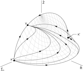
Figure 3: Orbits in the invariant set $\displaystyle\frac{\hat{\Omega}}{\hat{R}\hat{Z}}=2k$, $\gamma=1$.

Finally, we consider the case $\gamma=1$. By (2.12) the function $\chi$ defined in (2.11) describes a conserved quantity

$$\frac{\hat{\Omega}}{\hat{R}\hat{Z}}=2k,$$ (2.15)

where $k>0$ is a constant that depends on the initial conditions. We see that for all $k>0$ the surfaces described by (2.15) foliate the state space $S$ and intersect the vacuum boundary $\hat{\Omega}=0$ at $\hat{R}=0$ and $\hat{Z}=0$ (see figure 3).

We can use similar techniques from before to conclude that the equilibrium points $\mathsf{K}^{\pm}$ are asymptotically unstable. Since the orbits are constrained to lie on the two-dimensional family of invariant sets defined by (2.15), it follows that $\omega(\hat{\boldsymbol{x}})=\mathsf{V}$ for any $\hat{\boldsymbol{x}}\in S$. Thus any solution of the DE (2.6) in the set $S$ also satisfies (2.14) if $\gamma=1$.

Appendix B.2. Limits at late times of $(\bar{\Sigma}_{+},\bar{R},\bar{Z})$

We now apply theorem B.1 to prove (3.23), namely

$$\lim_{\tau\rightarrow+\infty}\bar{\boldsymbol{x}}=\boldsymbol{a},$$

where $\bar{\boldsymbol{x}}=(\bar{\Sigma}_{+},\bar{R},\bar{Z})$ and $\boldsymbol{a}=\left(\frac{1}{2},0,\frac{\sqrt{3}}{2}\right)$, considering the cases $1<\gamma\leqslant 2$ and $\gamma=1$ simultaneously.

We begin by defining the subset $D$ in theorem B.1 by

$$\Sigma_{+}^{2}+R^{2}+Z^{2}<1.$$

We now verify the hypotheses $H_{1}$ and $H_{2}$. Firstly, let $\boldsymbol{w}:[\tau_{0},+\infty)\rightarrow D$ be any $C^{0}[\tau_{0},\infty)$ function. Since $\lim_{\tau\rightarrow+\infty}M(\tau)=0$ it follows immediately that

$$\lim_{\tau\rightarrow+\infty}\boldsymbol{g}(\boldsymbol{w}(\tau),\tau)=\lim_{\tau\rightarrow+\infty}M(\tau)\left(B_{\bar{\Sigma}_{+}},\bar{R}B_{\bar{R}},\bar{Z}B_{\bar{Z}}\right)\Big{|}_{\bar{\boldsymbol{x}}=\boldsymbol{w}(\tau)}=\mathbf{0},$$

showing that $H_{1}$ is satisfied. Secondly, $H_{2}$ is satisfied since the variables $\bar{\Sigma}_{+}$, $\bar{R}$ and $\bar{Z}$ are bounded for all $\tau\geqslant\tau_{0}$ with $\tau_{0}$ sufficiently large. Therefore, since

$$\lim_{\tau\rightarrow+\infty}\hat{\boldsymbol{x}}(\tau)=\boldsymbol{a}$$

for all initial conditions $\hat{\boldsymbol{x}}(\tau_{0})$ in $D$ (see (2.14)), theorem B.1 implies that

$$\lim_{\tau\rightarrow+\infty}\bar{\boldsymbol{x}}(\tau)=\boldsymbol{a}$$ (2.16)

for all initial conditions $\bar{\boldsymbol{x}}(\tau_{0})$ in $D$.

Finally, we need to show that any initial condition $\boldsymbol{x}(\tau_{0})=(\Sigma_{+},R,Z)\big{|}_{\tau=\tau_{0}}$, $M(\tau_{0})$, $\psi(\tau_{0})$ for the DE (2.29), subject to $\Omega>0$ and (2.33), determines an initial condition $\bar{\boldsymbol{x}}(\tau_{0})$ in $D$ for the DE (3.18), so that (2.16) is satisfied.

Indeed, since $\lim_{\tau\rightarrow+\infty}\psi=+\infty$, we can without loss of generality restrict the initial condition $\psi(\tau_{0})$ to be a multiple of $\pi$. This requirement can be achieved by simply following the solution determined by the original initial condition until this condition is satisfied. It follows from this condition, in conjunction with (3.11) and the restriction $\Omega>0$ applied to (2.31), that

$$\left.\left(\bar{\Sigma}_{+}^{2}+\bar{R}^{2}+\bar{Z}^{2}\right)\right|_{\tau=\tau_{0}}=\left.\left(\Sigma_{+}^{2}+R^{2}+Z^{2}\right)\right|_{\tau=\tau_{0}}<1,$$

so that $\bar{\boldsymbol{x}}(\tau_{0})\in D$.

Appendix B.3. The limit of $M/R$ at late times

In analogy to (3.11), we define a variable $\bar{M}$ by

$$\bar{M}=M\left(1+{\textstyle\frac{1}{4}}R^{2}M\sin 2\psi\right).$$ (2.17)

It follows from (2.29) that the evolution equation for $\bar{M}$ is of the form

$$\bar{M}^{\prime}=-(\bar{Q}+2\bar{\Sigma}_{+}+MB_{\bar{M}})\bar{M},$$ (2.18)

where $B_{\bar{M}}$ is a bounded function for $\tau$ sufficiently large. By using (3.15) we obtain

$$\left(\frac{\bar{M}}{\bar{R}}\right)^{\prime}=\left(-{\textstyle\frac{3}{2}}+h(\bar{\boldsymbol{x}},M,\psi)\right)\left(\frac{\bar{M}}{\bar{R}}\right),$$ (2.19)

where

$$h(\bar{\boldsymbol{x}},M,\psi)={\textstyle\frac{5}{2}}-2\bar{Q}-3\bar{\Sigma}_{+}+MB_{*}$$

and $B_{*}$ is a bounded function for $\tau$ sufficiently large. It follows from (3.6), (3.11), (3.16) and theorem 3.5 that $\lim_{\tau\rightarrow+\infty}h(\bar{\boldsymbol{x}},M,\psi)=0$. Consequently, (2.19) implies that

$$\frac{\bar{M}}{\bar{R}}=\mathcal{O}\left(\rme^{(-3/2+\delta)\tau}\right),\qquad\text{if}\quad 1\leqslant\gamma\leqslant 2,$$ (2.20)

as $\tau\rightarrow+\infty$ for any $\delta>0$. Therefore, $\lim_{\tau\rightarrow+\infty}\bar{M}/\bar{R}=0$, which implies that $\lim_{\tau\rightarrow+\infty}M/R=0$, on account of (2.17) and (3.11).

Appendix C. Derivation of the asymptotic expansions (4.6) and (4.7)

In this appendix we give details of the derivation of the asymptotic expansions (4.6) and (4.7) for $\Sigma_{+}$, $R$, $Z$, $M$ and $\Omega$ as $\tau\rightarrow+\infty$. As was shown in appendix B.2, all solutions $\hat{\boldsymbol{x}}(\tau)$ of the DE (3.20) in the set $S$ (defined by (2.10)) are future asymptotic to the equilibrium point $(\hat{\Sigma}_{+},\hat{R},\hat{Z})=\left(\frac{1}{2},0,\frac{\sqrt{3}}{2}\right)$. Since this equilibrium point is non-hyperbolic, centre manifold theory is required in order to compute the decay rates of $\hat{\boldsymbol{x}}(\tau)$. In addition, the analysis has to be split into two cases, $1<\gamma\leqslant 2$ and $\gamma=1$, as described in appendices C.1 and C.2. We refer the reader to Carr (1981, pp 1–13) for an introductory discussion of centre manifold theory.

The next step is to show that the asymptotic expansions for $\hat{\boldsymbol{x}}(\tau)$ are compatible with the non-autonomous DE (3.18). In order to show this we need an asymptotic decay rate for $M$, which we obtain as follows. Equation (2.20) and the boundedness of $\bar{R}$ imply that $\bar{M}=\mathcal{O}(\rme^{(-3/2+\delta)\tau})$, as $\tau\rightarrow+\infty$, for any $\delta>0$. Using (2.17) we can conclude that

$$M=\mathcal{O}\left(\rme^{(-3/2+\delta)\tau}\right),$$ (3.1)

as $\tau\rightarrow+\infty$, for any $\delta>0$. We then write the non-autonomous DE (3.18) in integral form

$$\bar{\boldsymbol{x}}(\tau)=\bar{\boldsymbol{x}}(\tau_{0})+\int_{\tau_{0}}^{\tau}\left[\boldsymbol{f}(\bar{\boldsymbol{x}}(s))+\boldsymbol{g}(\bar{\boldsymbol{x}}(s),s)\right]\,\rmd s,$$ (3.2)

and can verify that the expansions for $\hat{\boldsymbol{x}}(\tau)$ are compatible with (3.2) using (3.19) and (3.1).

Appendix C.1. $1<\gamma\leqslant 2$

In order to put the DE (3.20) in the canonical form required for application of centre manifold theory, we begin by making the translation

$$(\hat{\Sigma}_{+},\hat{R},\hat{Z})=\left(y+{\textstyle\frac{1}{2}},x,z+{\textstyle\frac{\sqrt{3}}{2}}\right).$$ (3.3)

We can now apply theorem 3 in Carr (1981) to obtain an approximation to the local centre manifold through the point $(x,y,z)=(0,0,0)$ given by

$$\eqalign{y&=-x^{2}-2x^{4}-{\textstyle\frac{40}{3}}x^{6}+\mathcal{O}(x^{8}),\\ z&={\textstyle\frac{1}{\sqrt{3}}}x^{4}+{\textstyle\frac{28}{3\sqrt{3}}}x^{6}+\mathcal{O}(x^{8}).}$$ (3.6)

Upon applying theorem 1 in Carr (1981), we find that the governing DE for the flow on the centre manifold is given by

$$x^{\prime}=-2x^{3}-4x^{5}-32x^{7}+\mathcal{O}(x^{9}).$$ (3.7)

To obtain the asymptotic form of $x(\tau)$ from (3.7), we follow a procedure analogous to the one outlined in section 3.1 of Carr (1981) who considers a related problem. It follows that

$$x(\tau)=\frac{1}{2\tau}\left[1-\frac{1}{4\tau}(\ln\tau+C_{*})+\mathcal{O}(\tau^{-2}\ln^{2}\tau)\right],$$ (3.8)

as $\tau\rightarrow+\infty$, where $C_{*}$ is a constant that depends on the initial conditions (which can be set to zero upon appropriate translation of $\tau$). We have also included the second-order term in $x(\tau)$ so that the reader can compute the decay rates in section 4 to higher order if desired. The decay rates for $\hat{\Sigma}_{+}$, $\hat{R}$ and $\hat{Z}$ then follow from (3.3), (3.6) and (3.8) in conjunction with theorem 2 in Carr (1981). The compatibility check based on (3.1) and (3.2), in conjunction with the transformation (3.11), then lead to the given decay rates for $\Sigma_{+}$, $R$ and $Z$ in (4.6).

To obtain the asymptotic form of $M$ in (4.6), we substitute the known asymptotic expansions for $\bar{\boldsymbol{x}}(\tau)$ into the evolution equation (2.18) for $\bar{M}$, obtaining

$$\bar{M}^{\prime}=\left[-{\textstyle\frac{3}{2}}+{\textstyle\frac{3}{4}}\tau^{-1}\left(1+\mathcal{O}\left({\textstyle\frac{\ln\tau}{\tau}}\right)\right)\right]\bar{M},$$

on account of (3.1). We can now solve this DE and use (2.17) to obtain the decay rate for $M$.

Finally, to obtain the asymptotic expansion for $\Omega$, we define a variable $\bar{\Omega}$ according to

$$\bar{\Omega}=\Omega\left(1-{\textstyle\frac{1}{2}}R^{2}M\sin 2\psi\right).$$ (3.9)

It follows from (2.29) that the evolution equation for $\bar{\Omega}$ is of the form

$$\bar{\Omega}^{\prime}=[2\bar{Q}-(3\gamma-2)+MB_{\bar{\Omega}}]\bar{\Omega},$$

where $B_{\bar{\Omega}}$ is a bounded function for $\tau$ sufficiently large. Furthermore, using (3.15) we obtain

$$\left(\frac{\bar{\Omega}}{\bar{R}\bar{Z}}\right)^{\prime}=[-3(\gamma-1)+MB_{\ast}]\frac{\bar{\Omega}}{\bar{R}\bar{Z}}.$$

We can now solve this DE and then use the decay rates for $\bar{R}$ and $\bar{Z}$ and (3.9) to obtain the asymptotic expansion for $\Omega$ as stated in (4.7).

Appendix C.2. $\gamma=1$

Unlike the case $1<\gamma\leqslant 2$ where the centre manifold is one-dimensional, when $\gamma=1$ the centre manifold of the equilibrium point $(\hat{\Sigma}_{+},\hat{R},\hat{Z})=\left(\frac{1}{2},0,\frac{\sqrt{3}}{2}\right)$ is two-dimensional. Although the analysis is potentially more complicated, it can be reduced to a one-dimensional centre manifold problem by considering the DE (2.6) on the invariant surfaces $\hat{\Omega}/(\hat{R}\hat{Z})=2k$ (see (2.15)), where $k>0$ is a constant. Since, the analysis parallels that in appendix C.1 we only provide a brief outline of the proof. To begin, we use this first integral along with (2.8) to solve for $\hat{\Sigma}_{+}$ in terms of $\hat{R}$ and $\hat{Z}$ in a neighbourhood around $\hat{\Sigma}_{+}=\frac{1}{2}$ to obtain

$$\hat{\Sigma}_{+}=(1-2k\hat{R}\hat{Z}-\hat{R}^{2}-\hat{Z}^{2})^{1/2}.$$ (3.10)

Substituting (3.10) into the $\hat{R}$ and $\hat{Z}$ evolution equations in (2.6) and then making the transformation

$$\eqalign{\hat{R}&=x,\\ \hat{Z}&=-{\textstyle\frac{k}{2}}x+{\textstyle\frac{k}{2}}y+{\textstyle\frac{\sqrt{3}}{2}},}$$ (3.13)

puts the system into canonical form. We find that the centre manifold through the point $(x,y)=(0,0)$ is approximated by

$$y={\textstyle\frac{2}{3}}x^{3}+{\textstyle\frac{2\sqrt{3}}{9k}}(3+10k^{2})x^{4}+{\textstyle\frac{22}{3}}(2+k^{2})x^{5}+\mathcal{O}(x^{6}),$$ (3.14)

the corresponding DE on the centre manifold is

$$x^{\prime}=-\sqrt{3}\,kx^{2}+(k^{2}-2)\,x^{3}-2\sqrt{3}\,kx^{4}+\mathcal{O}(x^{5}),$$ (3.15)

and the asymptotic expansion for $x(\tau)$ is given by

$$x(\tau)=\frac{C_{R}}{\tau}\left[1+\frac{1}{3\tau}\left((1-6C_{R}^{2})\ln\tau+C_{*}\right)+\mathcal{O}(\tau^{-2}\ln^{2}\tau)\right],$$ (3.16)

as $\tau\rightarrow+\infty$, where $C_{*}$ is a constant that depends on the initial conditions. We note that the constant $C_{R}$ is related to the constant $k$ through $C_{R}=1/(\sqrt{3}\,k)$.

The asymptotic decay rates for $\hat{R}$ and $\hat{Z}$ follow from (3.13), (3.14) and (3.16), in conjunction with theorem 2 in Carr (1981). The expansion for $\hat{\Sigma}_{+}$ is obtained from (3.10). Dropping the hats as in appendix C.1 yields the decay rates for $\Sigma_{+}$, $R$ and $Z$ as stated in equation (4.6). The asymptotic form of $M$ is obtained in an analogous fashion to that outlined in appendix C.1. Finally, the asymptotic expansion for $\Omega$ as stated in (4.7) is obtained directly from (2.31).

Appendix D. The Weyl curvature tensor

In this appendix we give an expression for the Weyl curvature parameter $\mathcal{W}$ in terms of the Hubble-normalized variables $\Sigma_{+}$, $R$, $Z$, $M$ and $\psi$. Let $E_{\alpha\beta}$ and $H_{\alpha\beta}$ be the components of the electric and magnetic parts of the Weyl tensor relative to the group invariant frame with $\boldsymbol{e}_{0}=\boldsymbol{u}$. Since $E_{\alpha\beta}$ and $H_{\alpha\beta}$ are diagonal and trace-free (see WE, chapter 6, appendix), they each have two independent components. In analogy with (2.3) we define

$$\eqalign{\mathcal{E}_{+}={\textstyle\frac{1}{2}}(\mathcal{E}_{22}+\mathcal{E}_{33}),&\qquad\mathcal{E}_{-}={\textstyle\frac{1}{2\sqrt{3}}}(\mathcal{E}_{22}-\mathcal{E}_{33}),\\ \mathcal{H}_{+}={\textstyle\frac{1}{2}}(\mathcal{H}_{22}+\mathcal{H}_{33}),&\qquad\mathcal{H}_{-}={\textstyle\frac{1}{2\sqrt{3}}}(\mathcal{H}_{22}-\mathcal{H}_{33}),}$$ (4.3)

where $\mathcal{E}_{\alpha\beta}$ and $\mathcal{H}_{\alpha\beta}$ are the dimensionless counterparts of $E_{\alpha\beta}$ and $H_{\alpha\beta}$, defined by

$$\mathcal{E}_{\alpha\beta}=\frac{E_{\alpha\beta}}{H^{2}},\qquad\mathcal{H}_{\alpha\beta}=\frac{H_{\alpha\beta}}{H^{2}}.$$ (4.4)

It follows from (3.2), (4.3) and (4.4) that

$$\mathcal{W}^{2}=\mathcal{E}_{+}^{2}+\mathcal{E}_{-}^{2}+\mathcal{H}_{+}^{2}+\mathcal{H}_{-}^{2}.$$ (4.5)

The desired expressions for $\mathcal{E}_{\pm}$ and $\mathcal{H}_{\pm}$ can be obtained directly from equations (6.36) and (6.37) in WE, using (2.23) in the present paper:

$$\eqalign{\mathcal{E}_{+}&=\Sigma_{+}(1+\Sigma_{+})+{\textstyle\frac{1}{2}}R^{2}(1-3\cos 2\psi)-Z^{2}-3M^{2}Z^{4},\\ \mathcal{H}_{+}&=-{\textstyle\frac{3}{2}}R^{2}\sin 2\psi+{\textstyle\frac{9}{2}}M\Sigma_{+}Z^{2},\\ \mathcal{E}_{-}&=\frac{2R}{M}\left[\sin\psi+{\textstyle\frac{1}{2}}M(1-2\Sigma_{+})\cos\psi+{\textstyle\frac{3}{2}}M^{2}Z^{2}\sin\psi\right],\\ \mathcal{H}_{-}&=\frac{2R}{M}\left[-\cos\psi-{\textstyle\frac{3}{2}}M\Sigma_{+}\sin\psi-{\textstyle\frac{3}{4}}M^{2}Z^{2}\cos\psi\right].}$$ (4.10)

References