Abstract

In this paper the effect of the post-Newtonian gravitomagnetic force on the mean longitudes $l$ of a pair of counter-rotating Earth artificial satellites following almost identical circular equatorial orbits is investigated and the possibility of measuring it is examined. The observable is the difference of the times required for $l$ to pass from 0 to 2$\pi$ for both senses of motion. Such a gravitomagnetic time shift, which is independent of the orbital parameters of the satellites, amounts to 5$\times 10^{-7}$ s for the Earth; it is cumulative and should be measurable after a sufficiently high number of revolutions. The major limiting factors are the unavoidable imperfect cancellation of the Keplerian periods, which yields a constraint of 10^-2 cm in knowing the difference between the semimajor axes $a$ of the satellites, and the difference $I$ of the inclinations $i$ of the orbital planes which, for $i\sim 0.01^{\circ}$, should be less than $0.006^{\circ}$. A pair of spacecraft endowed with a sophisticated intersatellite tracking apparatus and drag-free control down to 10^-9 cm s^-2 Hz${}^{-\frac{1}{2}}$ level might allow to meet the stringent requirements posed by such a mission.

1 Introduction

The orbital path of a test particle freely falling in the gravitational field of a central body of mass $M$ and angular momentum $J$ is affected by various post-Newtonian general relativistic effects of order $\mathcal{O}(c^{-2})$[1, 2] like the Einstein gravitoelectric secular precession of the argument of pericentre $\omega$ [5] and the Lense-Thirring gravitomagnetic secular precessions of the longitude of the ascending node $\Omega$ and the argument of the pericentre $\omega$ [6].

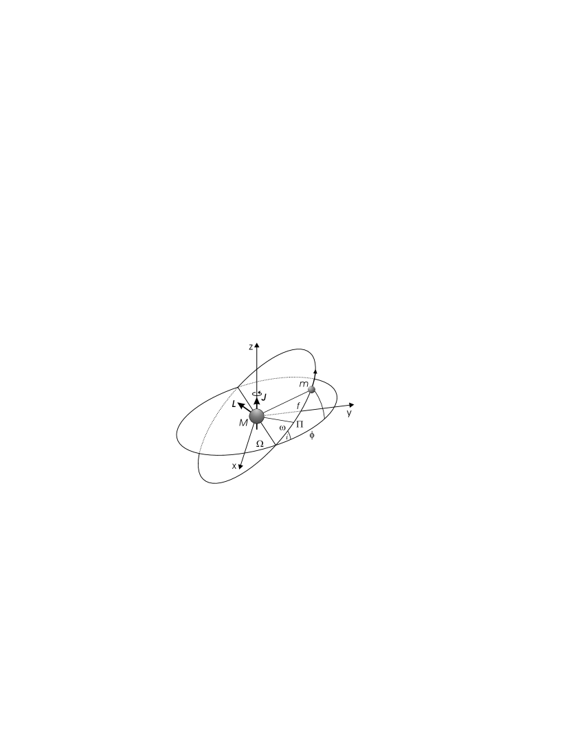
Figure 1: Orbital geometry for a motion around a central mass. Here $L$ denotes the orbital angular momentum of the particle of mass $m$, $J$ is the proper angular momentum of the central mass $M$, $\Pi$ denotes the pericentre position, $f$ is the true anomaly of $m$, which is counted from $\Pi$, $\Omega$, $\omega$ and $i$ are the longitude of the ascending node, the argument of pericentre and the inclination of the orbit with respect to the inertial frame $\{x,y,z\}$ and the azimuthal angle $\phi$ is the right ascension counted from the $x$ axis.

The Einstein precession is now known at a $10^{-4}$ level of relative accuracy, e.g., from Solar System planetary motions by analyzing more than 280,000 position observations (1913-2003) of different types including radiometric observations of planets and spacecrafts, CCD astrometric observations of the outer planets and their satellites, meridian transits and photographic observations [7]. On the contrary, to date there are not yet clear and undisputable direct tests of the various effects induced by the gravitomagnetic field. In April 2004 the Gravity Probe B (GP-B) mission [8] has been launched. Its goal is to measure, among other things, the gravitomagnetic precessions of the spins of four superconducting gyroscopes [9] carried onboard with a claimed accuracy of 1$\%$ or better. The Lense-Thirring effect on the orbits of the LAGEOS and LAGEOS II Earth’s artificial satellites has been experimentally checked for the first time some years ago with a claimed accuracy of the order of 20$\%$ [10], but, at present, there is not yet a full consensus on the real accuracy obtained in that test [11].

Recently, it has been shown that also the orbital period of a test particle is affected by the post-Newtonian gravitoelectromagnetic forces. The gravitomagnetic correction to the period of the (equatorial) right ascension $\alpha$, for $e=0$, $i=0^{\circ}$, where $e$ and $i$ are the eccentricity and the inclination, respectively, of the test particle’s orbit, has been worked out in [13]. The case of more general orbits has been treated in [14] ($e=0$, $i\neq 0^{\circ}$) and [15] ($e\neq 0$, $i\neq 0^{\circ}$). The gravitoelectric correction has been treated in [15]. Let us consider a pair of counter-orbiting satellites, conventionally denoted as $(+)$ and $(-)$, following identical circular and equatorial orbits along opposite directions around a central spinning body of mass $M$ and proper angular momentum $J$; while the gravitoelectric correction to the Keplerian period has the same sign for both the directions of motion, similar to the classical perturbing corrections of gravitational origin (oblateness of the central mass, tides, N-body interactions), the gravitomagnetic one changes its sign if the motion is reversed. This allows, at least in principle, to single out the latter one by measuring the difference of the periods of the counter-orbiting satellites. Some preliminary error analyses can be found in [16].

As we will show here, it turns out that also the mean longitudes $l=\mathcal{M}+\Omega+\omega$ are affected, among other perturbations, by the post-Newtonian general relativistic gravitoelectromagnetic forces. Also in this case the gravitomagnetic correction is sensitive to the direction of motion, contrary to the gravitoelectric one.

In this paper we will investigate the possibility of singling out the gravitomagnetic effect on the mean longitudes by means of a suitable space-based mission in the Earth space environment. We will mainly deal with a number of competing classical effects which could represent a source of systematic errors and bias. No measurements error budget is carried out.

2 The Gravitomagnetic Effect on the Mean Longitude

From the Gauss perturbative equations [17] it turns out that the rate equation for $l$, for small but finite values of $e$ and $i$, is

$$\frac{dl}{dt}\sim n-\frac{2}{na}A_{R}\left(\frac{r}{a}\right)+\left(\frac{i^{2}}{2}\right)\frac{d\Omega}{dt}+\left(\frac{e^{2}}{2}\right)\frac{d\omega}{dt},$$ (1)

where $a$ is the satellite’s semimajor axis and $n=(GMa^{-3})^{\frac{1}{2}}$ is the Keplerian mean motion; $A_{R}$ is the radial component of the perturbing acceleration ${\bf a}_{\rm pert}$. The currently available technologies allows to insert Earth artificial satellites in orbits with $e\lesssim 10^{-3}$ and $i\sim 0.01^{\circ}$; then, the third and fourth terms in eq.(1), which are proportional to $i$ and $e$ because $d\Omega/dt\propto 1/\sin i$ and $d\omega/dt\propto 1/e$, can be neglected and the equation

$$\frac{dl}{dt}\sim n-\frac{2}{na}A_{R}$$ (2)

can be used instead of eq.(1) to a good level of approximation.

According to [18], the radial components of the post-Newtonian general relativistic gravitoelectromagnetic accelerations, for generic orbits around a central spinning body, are

$$A_{R}^{\rm(GE)} = \frac{(GM)^{2}(1+e\cos f)^{2}}{c^{2}a^{3}(1-e^{2})^{3}}(3+2e\cos f-e^{2}+4e^{2}\sin^{2}f),$$ (3)

$$A_{R}^{\rm(GM)} = {2nGJ\cos i\over c^{2}a^{2}(1-e^{2})^{{7\over 2}}}(1+e\cos f)^{4},$$ (4)

where $f$ is the true anomaly. They are induced by the post-Newtonian general relativistic gravitoelectromagnetic fields

$${\bf E}^{\rm(GE)} = -\frac{GM}{c^{2}r^{3}}\left(\frac{4GM}{r}-{\bf v}^{2}\right)\mathbb{r}-\frac{4GM}{c^{2}r^{2}}(\mathbb{r}\cdot{\bf v}){\bf v},$$ (6)

$${\bf B}^{\rm(GM)} = -\frac{GJ}{cr^{3}}[{\bf\hat{J}}-3({\bf\hat{J}}\cdot{\bf\hat{r}}){\bf\hat{r}}].$$ (7)

From eq.(3)-eq.(4) it can be noted that, while the gravitoelectric acceleration is insensitive to the sense of motion of the test particle along its orbit, it is not so for the gravitomagnetic acceleration due to its dependence on $\cos i$. Indeed, according to [19]

$$\sin i = {(h_{x}^{2}+h_{y}^{2})^{{1\over 2}}\over\left|\ \bf h\right|},$$ (8)

$$\cos i = {h_{z}\over\left|\ \bf h\right|},$$ (9)

where ${\bf h}$ is the orbital angular momentum per unit mass whose components change sign when ${\bf v}\rightarrow-{\bf v}$. By reversing the sign of the velocity vector one obtains ($+$ and $-$ denote the pro- and retrograde orbits, respectively)

$$\sin i^{(-)} = \sin i^{(+)},$$ (10)

$$\cos i^{(-)} = -\cos i^{(+)},$$ (11)

from which it follows

$$i^{(-)}=180^{\circ}-i^{(+)}.$$ (12)

By inserting eq.(3)-eq.(4) in eq.(2), it can be obtained for the time $P_{l}$ required to $l$ for passing from 0 to 2$\pi$

$$P_{l}^{(\pm)}:=P_{l}^{(0)}+P_{l}^{(\rm GE)}+P_{l}^{(\rm GM)}=\frac{2\pi}{n}+\frac{12\pi(GMr_{0})^{\frac{1}{2}}}{c^{2}}\pm\frac{8\pi J}{c^{2}M}.$$ (13)

Eq.(13) yields for identical orbits followed in opposite directions,

$$\Delta P_{l}:=P_{l}^{(+)}-P_{l}^{(-)}={16\pi J\over c^{2}M},$$ (14)

which amounts to $5\times 10^{-7}$ s for Earth and is four times larger than the corresponding effect for the right ascension.

3 Sources of Systematic Errors

Eq.(14) would be valid only if the Keplerian periods (and the various classical and post-Newtonian gravitoelectric perturbative corrections to them) of the two satellites were exactly equal; this condition, however, cannot be achieved due to the unavoidable orbital injection errors. Then, eq.(14) has also to account for the difference induced in the Keplerian periods and the various classical and post-Newtonian gravitoelectric corrections to them, e.g., by the difference $d$ in the semimajor axes of the two satellites. The differences in $i$, which do not affect the Keplerian periods and the post-Newtonian gravitoelectric correction, would have, instead, an impact on the classical perturbative terms which cannot be neglected.

In general, the difference between the mean longitude periods of the two counter-rotating satellites can be written as

$$\Delta P_{l}=\Delta P^{(0)}+\Delta P_{l}^{\rm class}+\Delta P_{l}^{(\rm GE)}+\Delta P_{l}^{(\rm GM)}.$$ (15)

Over many orbital revolutions, say $N$, the accuracy in determining the gravitomagnetic time shift becomes

$$\delta[\Delta P^{(\rm GM)}]\leq{\delta(\Delta P)^{\rm exp}\over N}+\delta[\Delta P^{(0)}]+\delta[\Delta P_{l}^{\rm class}]+\delta[\Delta P_{l}^{\rm GE}],$$ (16)

where $\delta(\Delta P_{l})^{\rm exp}$ is the experimental error in the difference of the obtained $P_{l}^{(\pm)}$ over $N$ revolutions. After a sufficiently high number of orbital revolutions it should be possible to make the term ${\delta(\Delta P_{l})^{\rm exp}}/{N}$ smaller than $\Delta P_{l}^{(\rm GM)}$. In order to get an estimate, let us calculate the angular shift corresponding to $\Delta P_{l}^{(\rm GM)}$ over an orbital revolution by using

$$\frac{\Delta l}{\overline{l}}\sim\frac{\Delta P_{l}^{(\rm GM)}}{P_{l}^{(0)}}.$$ (17)

For $r_{0}=25498$ km and $P_{l}^{(0)}=4.05200895378\times 10^{4}$ s, $\overline{l}=2\pi$ the gravitomagnetic shift amounts to $\Delta l=1\times 10^{-2}$ milliarcseconds (mas in the following; 1 mas = 4.8$\times 10^{-9}$ rad), over an angular span. Since the accuracy with which the orientation of the axes of the International Terrestrial Reference System (ITRS) is of the order of 3 mas, after 300 orbital revolutions or 140 days, the gravitomagnetic time shift would reach this sensitivity cutoff.

3.1 The Impact of the Imperfect Cancellation of the Keplerian Periods

As we will see, the major limiting factor in measuring the gravitomagnetic time shift of interest is the difference of the Keplerian orbital periods

$$\Delta P^{(0)}={2\pi[r_{0}^{{3\over 2}}-(r_{0}+d)^{{3\over 2}}]\over(GM)^{{1\over 2}}}\sim{3\pi dr_{0}^{{1\over 2}}\over(GM)^{{1\over 2}}},$$ (18)

where $r_{0}$ represents the nominal value of the semimajor axis of the two satellites. The shift of eq.(18) cannot be made smaller than eq.(14), in practice, by choosing suitably the orbital geometry of the satellites. Indeed, from eq.(18) follows that the relation $d{r_{0}}^{{1\over 2}}\leq 1.059\times 10^{3}$ cm${}^{\frac{3}{2}}$ should be fulfilled; for $r_{0}\sim 10^{9}$ cm it would imply $d\sim 3\times 10^{-2}$ cm. Then, in order to be able to measure the relativistic effect of interest, which accumulates during the orbital revolution, the difference should be subtracted from the data provided that its error $\delta[\Delta P^{(0)}]$, which is present at every orbital revolution and is due to the uncertainties in the Earth $GM$, $r_{0}$ and $d$, is smaller than the gravitomagnetic time shift. This error is given by

$$\delta[\Delta P^{(0)}]\leq\left|{3\pi dr_{0}^{{1\over 2}}\over 2(GM)^{{3\over 2}}}\right|\times\delta(GM)+\left|{3\pi d\over 2(GMr_{0})^{{1\over 2}}}\right|\times(\delta r_{0})+\left|{3\pi r_{0}^{{1\over 2}}\over(GM)^{{1\over 2}}}\right|\times(\delta d)$$ (19)

and by assuming $r_{0}=25498$ km, $(\delta{r_{0}})^{\rm exp}=1$ cm and $\delta(GM)=8\times 10^{11}$ cm³ s^-2 [20], eq.(19) yields

$$\delta[\Delta P^{(0)}]\leq(2.8\times 10^{-14}\ {\rm cm^{-1}\ s})\times d+(2.3\times 10^{-5}\ {\rm cm^{-1}\ s})\times(\delta d).$$ (20)

Eq.(20) tells us that the error due to the uncertainty in $GM$ and, especially, $r_{0}$ is less than the gravitomagnetic effect, while $\delta d$ should be at the level of $2\times 10^{-2}$ cm. It seems to be impossible to meet this very stringent requirement with the current SLR technology due to many measurement errors (station errors, random errors in precession, nutation and Earth rotation, observation errors). However, an intersatellite tracking approach could yield better results. A level of $(\delta d)^{\rm exp}$ of the order of $10^{-3}$ cm is currently available with the K-band Ranging (KBR) intersatellite tracking technology used for the GRACE mission [21]. On the other hand, it must be noted that it would not be easy to use this approach for satellites following opposite directions. The GRACE twins revolve in the same sense.

In regard to $(\delta d)^{\rm systematic}$, thinking about a pair of completely passive, spherical LAGEOS–like satellites, it should be pointed out that for orbits with $e\sim i\sim 0$, for which eq.(14) holds, many non–gravitational perturbations affecting the semimajor axis vanish [22]; the remaining ones could be strongly constrained by constructing the two satellites very carefully with regard to their geometrical and physical properties. Some figures will be helpful. We will adopt the physical properties of the existing LAGEOS satellites. The atmospheric drag induces a decrease in the semimajor axis of $\Delta a=-a^{2}\varrho C_{D}S/m$ over one orbital revolution, where $C_{D}$ is the satellite drag coefficient, $S/m$ is the satellite area-to-mass ratio and $\varrho$ is the atmospheric density at the satellite altitude. For $C_{D}\sim 4.9$, $S/m=7\times 10^{-3}$ cm² g^-1 and $\varrho=8.4\times 10^{-21}$ g cm^-3 (estimate of the atmospheric neutral density at LAGEOS altitude; for $r_{0}=25498$ km it should be smaller, of course) the decrease in the semimajor axis amounts to 4$\times 10^{-4}$ cm over one orbital revolution. The impact of direct solar radiation pressure on the semimajor axis of a circular orbit vanishes, also when eclipses effects are accounted for. The nominal Poynting-Robertson effect on the semimajor axis of a circular, equatorial orbit ($r_{0}=25498$ km) is of the order of $10^{-3}$ cm over one orbital revolution. However, it is linearly proportional to the satellite reflectivity coefficient $C_{R}$ for which a 0.5–1$\%$ mismodelling can be assumed. The semimajor axis of a circular orbit is neither affected neither the albedo over one orbital revolution. The same holds also for the IR Earth radiation pressure and the solar Yarkovsky-Schach effect (by neglecting the eclipses effects). The Earth Yarkovsky-Rubincam effect would affect the semimajor axis of an orbit with $i\sim 0^{\circ}$ by means of a nominal secular trend less than $1\times 10^{-1}$ cm ($r_{0}=25498$ km) over one orbital revolution. However, a 20-25$\%$ mismodelling can be assumed on it. The direct effect of the terrestrial magnetic field on the semimajor axis of a circular orbit vanishes over one orbital revolution.

Another possibility could be the use of more complex (and more expensive) spacecraft endowed with a drag–free apparatus; it would be helpful in suitably constraining $(\delta{r_{0}})^{\rm systematic}$ and, especially, $(\delta d)^{\rm systematic}$. Indeed, for orbits with semimajor axis of the order of 10⁹ cm the unperturbed Keplerian period is of the order of $P^{(0)}\sim 4\times 10^{4}$ s. If the maximum admissible error in knowing the position of the satellites is of the order of $2\times 10^{-2}$ cm then the maximum disturbing acceleration that would not mask the gravitomagnetic clock effect, over one orbital revolution, is $\delta d/[P^{(0)}]^{2}\sim 1\times 10^{-11}$ cm s^-2. But the drag–free technologies currently under development for LISA [23] and OPTIS [24] missions should allow to cancel out the accelerations of non–gravitational origin down to $3\times 10^{-13}$ cm s^-2 Hz${}^{-{\frac{1}{2}}}$ and 10^-12 cm s^-2 Hz${}^{-{\frac{1}{2}}}$, respectively. In our case, for $r_{0}=25498$ km and an orbital frequency of $2.4\times 10^{-5}$ Hz, a $1\times 10^{-9}$ cm s^-2 Hz${}^{-\frac{1}{2}}$ drag-free level would be sufficient. More precisely, from the Gauss perturbative rate equation of the semimajor axis it turns out that, for circular orbits, the effects induced on $r_{0}$ by periodically time-varying non–gravitational along-track accelerations with frequencies multiple of the orbital frequency vanish over one orbital revolution. For constant along-track accelerations $A_{T}$ the situation is different: over one orbital revolution (corresponding to a frequency of the order of 10^-5 Hz) their effect on $r_{0}$ would amount to

$$\delta r_{0}^{(\rm NG)}=4\pi\left(\frac{r_{0}^{3}}{GM}\right)A_{T}.$$ (21)

In order to make $\delta r_{0}^{(\rm NG)}=2\times 10^{-2}$ cm the maximum value for $A_{T}$ would be $3.8\times 10^{-11}$ cm s^-2 in a frequency range with $10^{-5}$ Hz as upper limit. It is a difficult but not impossible limit to be obtained with the drag-free technologies which are currently under development.

3.2 The Impact of the Imperfect Cancellation of the Post-Newtonian Gravitoelectric Periods

The perturbative correction to $P_{l}$ induced by the post-Newtonian gravitoelectric acceleration, given in eq.(14), amounts to

$$P_{l}^{(\rm GE)}=\frac{12\pi(GMr_{0})^{\frac{1}{2}}}{c^{2}}.$$ (22)

For an Earth high-orbit satellite it is of the order of 10^-5 s. The orbital injection errors in $r_{0}$ would yield

$$\Delta P_{l}^{(\rm GE)}\sim\frac{6\pi}{c^{2}}\left(\frac{GM}{r_{0}}\right)^{\frac{1}{2}}d,$$ (23)

which amounts to 10^-9 s for $r_{0}=25498$ km and $d=5$ km. This result justifies, a posteriori, our choice of neglecting the small corrections to eq.(22) induced by the small, but finite, eccentricity of the orbit.

3.3 The Impact of the Classical Gravitational Perturbations

In this section the perturbations of gravitational origin on the mean longitude $l$ and their impact on the measurement of $\Delta P^{(\rm GM)}_{l}$ are investigated.

3.3.1 The Geopotential

Since we are interested in effects which are averaged over many orbital revolutions, only the zonal harmonics of geopotential, which induces secular perturbations on $\Omega,\ \omega$ and $\mathcal{M}$, will be considered. In the following the Gaussian approach together with eq.(2) will be used.

Let us write the zonal part of geopotential as

$$\Phi^{\rm zon}:=\Phi^{(0)}+\Delta\Phi^{\rm zon}={GM\over r}-GM\sum^{\infty}_{\ell=2}\frac{R^{\ell}_{\oplus}}{r^{\ell+1}}\ J_{\ell}\ P_{\ell}(\cos\theta).$$ (24)

According to (6.98b) of [25], the radial component of the perturbing acceleration, in spherical coordinates, for an even zonal harmonic of degree $\ell$, is

$$A_{R}^{(J_{\ell})}={\partial{\Delta\Phi^{\rm zon}}\over\partial{r}}=(\ell+1){GMR_{\oplus}^{\ell}\over r^{\ell+2}}\ J_{\ell}\ P_{\ell}(\cos\theta).$$ (25)

It is easy to see that the odd zonal harmonics of geopotential do not affect the mean longitude of a satellite in an equatorial orbit. Indeed, it is well known that the odd-degree Legendre polynomials vanish for $\theta=90^{\circ}$ [26]. The perturbing radial accelerations due to the even zonal harmonics are

$$A_{R}^{(J_{2})} = -{3GMR^{2}_{\oplus}J_{2}\over 2r^{4}},$$ (26)

$$A_{R}^{(J_{4})} = {15GMR^{4}_{\oplus}J_{4}\over 8r^{6}},$$ (27)

$$A_{R}^{(J_{6})} = -{35GMR^{6}_{\oplus}J_{6}\over 16r^{8}},$$ (28)

$$A_{R}^{(J_{8})} = {315GMR^{8}_{\oplus}J_{8}\over 128r^{10}}.$$ (29)

Inserting eq.(26)-eq.(29) in eq.(2) yields

$$P_{l}^{\rm obl}=-{6\pi R^{2}_{\oplus}J_{2}\over(GMr_{0})^{\frac{1}{2}}}+{15\pi R^{4}_{\oplus}J_{4}\over(GMr^{5}_{0})^{\frac{1}{2}}}-{35\pi R^{6}_{\oplus}J_{6}\over 4(GMr^{9}_{0})^{\frac{1}{2}}}+{315\pi R_{\oplus}^{8}J_{8}\over 32(GMr_{0}^{13})^{{1\over 2}}}-...=$$

$$=-8.2341063\ {\rm s}-1.9266\times 10^{-3}\ {\rm s}-2.34\times 10^{-5}\ {\rm s}+5\times 10^{-7}\ {\rm s}+...$$ (30)

for an orbit radius $r_{0}=25498$ km. This shows that, for such a radius, just the first four even zonal harmonics are of the same order of magnitude of $P_{l}^{(\rm GM)}\sim 10^{-7}$ s.

Let us now evaluate the impact of the even zonal harmonics the geopotential on the measurement of $\Delta P_{l}^{(\rm GM)}$ for a pair of counter-orbiting satellites whose orbits differ by a small amount $d\ll r_{0}$ in radius. With

$$\frac{1}{(r_{0})^{\frac{n}{2}}}-\frac{1}{(r_{0}+d)^{\frac{n}{2}}}\sim\frac{nd}{2(r_{0})^{\frac{n+2}{2}}},$$ (31)

the difference in the perturbing terms due to the even zonal harmonics are, for $d=5$ km and $r_{0}=25498$ km

$$\Delta P_{l}^{(J_{2})} = -{3\pi R^{2}_{\oplus}J_{2}d\over(GMr_{0}^{3})^{\frac{1}{2}}}=-8.068\times 10^{-4}\ {\rm s},$$ (32)

$$\Delta P_{l}^{(J_{4})} = {75\pi R^{4}_{\oplus}J_{4}d\over 2(GMr_{0}^{7})^{\frac{1}{2}}}=-9\times 10^{-7}\ {\rm s},$$ (33)

$$\Delta P_{l}^{(J_{6})} = -{315\pi R^{6}_{\oplus}J_{6}d\over 8(GMr_{0}^{11})^{\frac{1}{2}}}=-2\times 10^{-8}\ {\rm s},$$ (34)

$$\Delta P_{l}^{(J_{8})} = {4095\pi R^{8}_{\oplus}J_{8}d\over 64(GMr_{0}^{15})^{\frac{1}{2}}}=6\times 10^{-10}\ {\rm s}.$$ (35)

This means that only $\Delta P_{l}^{(J_{2})}$ and $\Delta P_{l}^{(J_{4})}$ are relevant. The uncertainty in the knowledge of the Earth $GM$ and of the even zonal harmonics yield

$$\delta[\Delta P_{l}^{(J_{2})}]_{GM} = {3\pi R^{2}_{\oplus}J_{2}d\over 2(GMr_{0})^{\frac{3}{2}}}\times\delta(GM)\sim 8\times 10^{-13}\ {\rm s},$$ (36)

$$\delta[\Delta P_{l}^{(J_{2})}]_{J_{2}} = {3\pi R^{2}_{\oplus}d\over(GMr_{0}^{3})^{\frac{1}{2}}}\times(\delta J_{2})\sim 3\times 10^{-11}\ {\rm s},$$ (37)

$$\delta[\Delta P_{l}^{(J_{4})}]_{GM} = {75\pi R^{4}_{\oplus}J_{4}d\over 4(GM)^{\frac{3}{2}}(r_{0})^{\frac{7}{2}}}\times\delta(GM)\sim 9\times 10^{-16}\ {\rm s},$$ (38)

$$\delta[\Delta P_{l}^{(J_{4})}]_{J_{4}} = {75\pi R^{4}_{\oplus}d\over 2(GMr_{0}^{7})^{\frac{1}{2}}}\times(\delta J_{4})\sim 3\times 10^{-11}\ {\rm s},$$ (39)

For $\delta(GM)$ and $\delta J_{\ell}$ the values of the IERS convention [20] and of the EIGEN-2 Earth gravity model [27], respectively, have been used.

Another source of error is represented by the uncertainty in the knowledge of the separation $d$ between the two orbits and of their radius $r_{0}$. Their impact is, by assuming $\delta d\sim\delta r_{0}\sim 1$ cm

$$\delta[\Delta P_{l}^{(J_{2})}]_{r_{0}} = {9\pi R^{2}_{\oplus}J_{2}d\over 2(GM)^{\frac{1}{2}}(r_{0})^{\frac{5}{2}}}\times(\delta r_{0})\sim 4\times 10^{-13}\ {\rm s},$$ (40)

$$\delta[\Delta P_{l}^{(J_{2})}]_{d} = {3\pi R^{2}_{\oplus}J_{2}\over(GMr_{0}^{3})^{\frac{1}{2}}}\times(\delta d)\sim 1\times 10^{-9}\ {\rm s},$$ (41)

$$\delta[\Delta P_{l}^{(J_{4})}]_{r_{0}} = {525\pi R^{4}_{\oplus}J_{4}d\over 4(GM)^{\frac{1}{2}}(r_{0})^{\frac{9}{2}}}\times(\delta r_{0})\sim 1\times 10^{-15}\ {\rm s},$$ (42)

$$\delta[\Delta P_{l}^{(J_{4})}]_{d} = {75\pi R^{4}_{\oplus}J_{4}\over 2(GMr_{0}^{7})^{\frac{1}{2}}}\times(\delta d)\sim 2\times 10^{-12}\ {\rm s},$$ (43)

These results clearly show that, for the same semimajor axis of, say, the ETALON SLR satellites and for not too stringent requirements on the orbital injection errors for the separation between the two orbits, the impact of the geopotential on the measurement of $\Delta P_{l}^{(\rm GM)}$ is negligible.

Finally, let us consider what could be the impact of the secular variations of the even zonal harmonics $\dot{J}_{\ell}$. For the first even zonal harmonic the effective $\dot{J}_{2}^{\rm eff}\sim\dot{J}_{2}+0.371\dot{J}_{4}+0.079\dot{J}_{6}+0.006\dot{J}_{8}-0.003\dot{J}_{10}...$, whose magnitude is of the order of $(-2.6\pm 0.3)\times 10^{-11}$ yr^-1, can be considered. The insertion of such value in eq.(32) yields $\Delta P_{l}^{(\dot{J}_{2}^{\rm eff})}=1\times 10^{-11}$ s over one year, so that it can be concluded that its effect can be safely neglected.

3.3.2 The Tides

Another source of potential systematic error is represented by the solid Earth and ocean tides [29].

For a constituent of given frequency ${\rm f}$ of the solid Earth tidal spectrum, which is the more effective in perturbing the Earth satellites’orbits, the perturbation of degree $\ell$ and order $m$ induced on $l$ is

$$\frac{dl}{dt}=n+A_{\ell m}(GM)^{\frac{1}{2}}R^{\ell-1}_{\oplus}r_{0}^{-(\frac{2\ell+3}{2})}2(\ell+1)\sum_{p=0}^{\ell}\sum_{q=-\infty}^{+\infty}F_{\ell mp}G_{\ell pq}k_{\ell m}^{(0)}H_{\ell}^{m}\cos\gamma_{{\rm f}\ell mpq},$$ (44)

where $A_{\ell m}=[(2\ell+1)(\ell-m)!/(4\pi)(\ell+m)!]^{\frac{1}{2}}$, $F_{\ell mp}(i)$ and $G_{\ell pq}(e)$ are the inclination and eccentricity functions, respectively [4], $k_{\ell m}^{(0)}$ are the Love numbers, $H_{\ell}^{m}$ are the tidal heights and $\gamma_{{\rm f}\ell mpq}$ is built up with the satellite’s orbital elements $\Omega$, $\omega$ and $\mathcal{M}$, the lunisolar variables and the lag angle $\delta_{{\rm f}\ell m}$ [29]. Note that the dependence on $F_{\ell mp}$ and $G_{\ell pq}$ is the same also for the ocean tidal perturbations.

From an inspection of the explicit expressions of the inclination and eccentricity functions [4] and from the condition $\ell-2p+q=0$, which must be fulfilled for the perturbations averaged over an orbital revolution, it turns out that the $\ell=3$ part of the entire tidal spectrum does not affect the mean longitude of a satellite with $i=e=0$. With regard to the $\ell=2$ constituents, only the long-period zonal ($m=0$) tides induce non vanishing perturbations on $P_{l}$ for circular and equatorial orbits. Among them, the most powerful is by far the 18.6-year lunar tide. Its effect on $P_{l}$ is given by

$$P_{l}^{(\rm 18.6-yr)}=\frac{3(5\pi)^{\frac{1}{2}}\ R_{\oplus}\ k^{(0)}_{20}(\bar{\rm f})\ H_{2}^{0}(\bar{\rm f})}{(GMr_{0})^{\frac{1}{2}}}\cos\gamma_{{\bar{\rm f}}2010}.$$ (45)

For $r_{0}=25498$ km it amounts to 3$\times 10^{-6}$ s. The difference in the orbits of the two satellites would yield

$$\Delta P_{l}^{(\rm 18.6-yr)}=\frac{3(5\pi)^{\frac{1}{2}}\ R_{\oplus}\ k^{(0)}_{20}(\bar{\rm f})\ H_{2}^{0}(\bar{\rm f})\ d}{2(GMr_{0}^{3})^{\frac{1}{2}}}\cos\gamma_{{\bar{\rm f}}2010}\sim 6\times 10^{-10}\ {\rm s}$$ (46)

for $d=5$ km and $r_{0}=25498$ km. As can be seen, $\Delta P_{l}^{(\rm GM)}\gg\Delta P_{l}^{(\rm 18.6-yr)}$, so that the impact of the direct tidal perturbations on the measurement of the gravitomagnetic clock effect on $l$ can be neglected.

The cross-coupling between the static Earth oblateness and the Earth tides [33] would induce the following perturbations on the mean longitude

$$\frac{dl}{dt}=n-\frac{21J_{2}GMR_{\oplus}^{\ell+1}A_{\ell m}\sum_{p=0}^{\ell}\sum_{q=-\infty}^{+\infty}F_{\ell mp}G_{\ell pq}[(\ell-2p)-m]k^{(0)}_{\ell m}H_{\ell}^{m}}{2r_{0}^{\ell+5}{\rm f}}\cos\gamma_{{\rm f}\ell mpq}.$$ (47)

From an inspection of the explicit expressions of the inclination functions (see Appendix A) and from the condition $\ell-2p=0$, which holds for even $\ell$, it turns out that the $\ell=2$ part of the indirect tidal spectrum, which is the most powerful, has no effect on $l$ for an equatorial orbit. More precisely, $F_{201}$ does not vanish for $i=0^{\circ}$, but in this case, $\ell-2p=m=0$. The other $\ell=2$ inclination functions vanish for equatorial orbits. The same holds also for the $\ell=3$ constituents for which $\ell-2p\neq 0$. It turns out that $F_{311}\neq 0$ for equatorial orbits; in this case $\ell-2p=m=1$. The other $\ell=3$ inclination functions vanish for $i=0^{\circ}$.

3.3.3 The Impact of the Errors in the Inclinations

Until now we have propagated the uncertainties in the orbit radius by assuming for the inclination and the eccentricity their nominal values $i=e=0$. Now we wish to fix $r_{0}$ and propagate the errors in the inclination [34]. As pointed out before, the uncertainties in $i$ affect the classical perturbative corrections to the Keplerian periods. The effects of the Earth oblateness are the most prominent; thus, we will investigate them in order to establish upper bounds in the admissible separation $I$ between the two orbital planes.

The radial component of the perturbing acceleration due to $J_{2}$ for a generic orbit reads

$$A_{R}^{(J_{2})}=-\frac{3GMR_{\oplus}^{2}J_{2}}{4r^{4}}\left[3\cos 2(\omega+f)+3\cos^{2}i-3\cos^{2}i\cos 2(\omega+f)-1\right].$$ (48)

Neglecting all terms of order $\mathcal{O}(e^{2})$, eq.(48) in eq.(2) yields

$$P_{l}^{(J_{2})}=\frac{3\pi R^{2}_{\oplus}J_{2}}{(GMr_{0})^{\frac{1}{2}}}(1-3\cos^{2}i).$$ (49)

Then, for the counter-orbiting satellites along identical (almost) circular orbits with inclinations $i^{(+)}\equiv i$ and $i^{(-)}=(180^{\circ}-i)+I$, with $I/i\ll 1$, from $\cos^{2}i\sim 1+i^{2}$,

$$\Delta P_{l}^{(J_{2})}\sim\frac{18\pi R^{2}_{\oplus}J_{2}}{(GMr_{0})^{\frac{1}{2}}}(iI).$$ (50)

For $r_{0}=25498$ km and $i=0.01^{\circ}$, $\Delta P_{l}^{(J_{2})}\leq\Delta P_{l}^{(\rm GM)}$ if $I\leq 0.006^{\circ}=1\times 10^{-4}$ rad. It is worth noting that the current technology does allow to obtain equatorial orbits tilted by $0.01^{\circ}$ to the equator, e.g., for many geostationary satellites. Many orbital perturbations affect the inclination with shifts $\Delta i$ which must be kept smaller than $I$. The static part of geopotential does not induce long-term perturbations on the inclinations. The tesseral and sectorial solid Earth and ocean tides induces long-period perturbations on $i$ of the order of a few tens of mas. The general relativistic gravitoelectric de Sitter, or geodetic, precession [35] induces a secular variation of the inclination of 84 mas yr^-1. The inclination is sensitive to the non-gravitational perturbations, but the drag-free apparatus could resolve this problem. Suffices it to say that the uncancelled non-conservative perturbations on $i$ for the LAGEOS satellites amount to a few tens of mas yr^-1 [36]. It is also important to note that departures of $i$ from their nominal values of the order of $I\sim 0.0001^{\circ}$ are feasible with the current technologies for, e.g., the planned GP-B mission [37, 38] and the current GRACE mission. It turns out that the requirements on the semimajor axis and the eccentricity are far less demanding than those on the inclination [34].

3.3.4 The N-Body Gravitational Perturbations

Another source of perturbations on an Earth satellite’s mean longitude is represented by the gravitational effect induced by the major bodies of the Solar System (Sun, Moon, Jupiter, other planets, the asteroids). Let us calculate the effects induced by some of them.

The perturbative effect of the planet of mass $m^{{}^{\prime}}$ on the satellite of mass $m$ is given by [25]

$$\mathcal{R}_{\rm planets}=Gm^{{}^{\prime}}\left({1\over|\bf r-\bf r^{{}^{\prime}}|}-{{\bf r}\cdot{\bf r}^{{}^{\prime}}\over r^{{}^{\prime}3}}\right).$$ (52)

It turns out that the second term in eq.(52) does not induces secular perturbations.

After expressing the first term of eq.(52) in terms of the orbital elements of the satellite and the planet and averaging it over one period of the mean longitudes $l$ and $l^{{}^{\prime}}$ one finds for the largest contribution which does not contain the terms of second order in the eccentricities and the inclinations

$$P_{l}^{(\rm planets)}=-{4\pi Gm^{{}^{\prime}}\over n^{3}a^{{}^{\prime}3}}.$$ (53)

It is important to notice that eq.(53) does not depend on the sense of motion along the orbits, so that it cancels, in principle, in $\Delta P_{l}$. Instead, the difference $d$ in the semimajor axes of the two satellites would induce an aliasing effect

$$\Delta P_{l}^{\rm(planets)}\sim\frac{18\pi m^{{}^{\prime}}da^{\frac{7}{2}}}{G^{\frac{1}{2}}a^{{}^{\prime}3}M_{\oplus}^{\frac{3}{2}}}.$$ (54)

The nominal values of eq.(54) for the Sun and the Moon amount to 1.178$\times 10^{-4}$ s and $2.565\times 10^{-4}$ s, respectively. However, the uncertainties in $Gm^{{}^{\prime}}$ yield

$$\delta[\Delta P_{l}^{\rm(Sun)}]_{GM_{\odot}} = 7\times 10^{-15}\ {\rm s},$$ (55)

$$\delta[\Delta P_{l}^{\rm(Moon)}]_{Gm_{\rm Moon}} = 6\times 10^{-11}\ {\rm s},$$ (56)

where we have used $\delta(GM)_{\odot}=8\times 10^{-9}$ m³ s^-2 [30] and $\delta(Gm)_{\rm Moon}=1.2\times 10^{-6}$ m³ s^-2 [31]. The errors induced by the uncertainties in $d$, $a$ and $GM_{\oplus}$ turn out to be negligible. The corrections $\Delta P_{l}^{\rm(planets)}$ for Venus, Mars, Jupiter and Ceres, whose mass amounts to approximately one third of the total mass of asteroids $m^{\rm asteroids}=2.3\times 10^{24}$ g, are negligible because their nominal values are $\leq 10^{-9}$ s. This is particularly important for Jupiter, whose contribution would amount to $\Delta P_{l}^{\rm(Jup)}=1\times 10^{-9}$ s, because its sidereal orbital period, with respect to the Sun, amount to almost 11 years.

It can be shown that the indirect effect induced on $P^{(0)}$ by the perturbations on $a$ can be neglected. Indeed, there are no N-body secular perturbations on $a$ and, most importantly, their amplitudes are proportional to factors like $e^{|h_{1}|}e^{{}^{\prime}|h_{2}|}\sin^{|h_{3}|}i\sin^{|h_{4}|}i^{{}^{\prime}}$, where $h_{1},\ h_{2},\ h_{3}$ and $h_{4}$ are integer numbers [32] constrained by the conditions $|h_{1}|+|h_{2}|+|h_{3}|+|h_{4}|\leq 2$ and, for the short–period perturbations, $h_{1}+h_{2}+h_{3}+h_{4}\neq 0$.

3.4 The Impact of the Non-Gravitational Perturbations

From eq.(2) it turns out that, in general, periodically time-varying radial accelerations with frequencies multiple of the orbital frequency do not affect the mean longitude over an orbital revolution, at least at order $\mathcal{O}(e)$.

The situation is different for radial accelerations which can be considered constant in time over an orbital revolution. Let us consider an acceleration of non–gravitational origin whose radial component $A_{R}$ is constant over the timescale of one orbital revolution. From eq.(2) it turns out that

$$P_{l}^{(\rm NG)}=4\pi\left(\frac{r_{0}^{7}}{GM^{3}}\right)^{\frac{1}{2}}A_{R},$$ (57)

from which it follows

$$\Delta P_{l}^{(\rm NG)}=14\pi d\left(\frac{r_{0}^{5}}{GM^{3}}\right)^{\frac{1}{2}}A_{R}.$$ (58)

The maximum value of $A_{R}$ which makes $\Delta P_{l}^{(\rm NG)}\leq\Delta P_{l}^{(\rm GM)}$ is $A_{R}^{\rm max}=6\times 10^{-7}$ cm s^-2 for $d=5$ km and $r_{0}=25498$ km. It is not a too stringent constraint. For LAGEOS, which is completely passive, the largest non–gravitational acceleration, i.e. the direct solar radiation pressure, amounts to almost $4\times 10^{-7}$ cm s^-2; a drag-free apparatus with not too stringent performances–well far from the $10^{-13}$ cm s^-2 Hz${}^{-\frac{1}{2}}$ level of LISA–could meet in a relatively easy way such requirement. For $\delta d\sim\delta r_{0}\sim 1$ cm, $\delta(GM)=8\times 10^{11}$ cm³ s^-2 and $A_{R}=6\times 10^{-7}$ cm s^-2 it turns out

$$\delta[\Delta P_{l}^{(\rm NG)}]_{d} = 14\pi\left(\frac{r_{0}^{5}}{GM^{3}}\right)^{\frac{1}{2}}A_{R}\times(\delta d)=1\times 10^{-12}\ {\rm s},$$ (59)

$$\delta[\Delta P_{l}^{(\rm NG)}]_{r_{0}} = 35\pi d\left(\frac{r_{0}}{GM}\right)^{\frac{3}{2}}A_{R}\times(\delta r_{0})=5\times 10^{-16}\ {\rm s},$$ (60)

$$\delta[\Delta P_{l}^{(\rm NG)}]_{GM} = 21\pi d\left(\frac{r_{0}}{GM}\right)^{\frac{5}{2}}A_{R}\times\delta(GM)=1\times 10^{-15}\ {\rm s}.$$ (61)

These results show that the direct impact of the non-gravitational accelerations on the measurement of the gravitomagnetic time shift on $l$ could be made negligible with a drag-free apparatus of relatively modest performances, contrary to the indirect effects on the difference of the Keplerian periods which, as seen before, would require a much more effective drag–free cancellation in the frequency range $[0,\ 10^{-5}\ {\rm Hz}]$.

4 Conclusions

In this paper we have examined the possibility of measuring the gravitomagnetic clock effect on the mean longitudes of a pair of counter-rotating satellites following almost identical circular equatorial orbits in the gravitational field of Earth. While the gravitomagnetic signature depends only on the Earth parameters, the aliasing classical effects depend also on the orbital geometry of the satellites, so that it is possible to choose it suitably in order to reduce their impact on the measurement of the post-Newtonian effect. In this respect, our choice of a nominal value of 25498 km for the semimajor axis yields good results.

From the point of view of the observational accuracy, one source of error would be the uncertainty with which the axes of the ITRS are known. However, it turns out that the level of the gravitomagnetic effect can be reached over a sufficiently high number of orbital revolutions.

In regard to the systematic errors, the major limiting factors are

• The unavoidable imperfect cancellation of the Keplerian periods, which yields a 10^-2 cm constraint in knowing the difference $d$ between the semimajor axes of the satellites

• The required accuracy in the knowledge of the inclinations $i$ of the satellites in presence of not exactly equatorial orbits. For $i=0.01^{\circ}$ the difference between the inclinations of the two orbital planes $I\equiv i^{(+)}-i^{(-)}$ should be less than 0.006^∘.

A pair of drag-free ($10^{-9}$ cm s^-2 Hz${}^{-\frac{1}{2}}$) spacecraft endowed with an intersatellite tracking apparatus might allow to meet the stringent requirements of such a mission whose realization seems to be very difficult although, perhaps, not completely impossible with the present-day or forthcoming space technologies.

References

- [1] I. Ciufolini and J.A. Wheeler, Gravitation and Inertia (Princeton University Press, Princeton, 1995).
- [2] B. Mashhoon, F. Gronwald and H.I.M. Lichtenegger, in: Gyros, Clocks, Interferometers…:Testing Relativistic Gravity in Space, edited by C. Lämmerzahl, C.W.F. Everitt and F.W. Hehl (Springer, Berlin, 2001), pp. 83-108.
- [3] W.M. Kaula, Theory of Satellite Geodesy (Blaisdell, Waltham, 1966).
- [4] W.M. Kaula, Theory of Satellite Geodesy (Blaisdell, Waltham, 1966).
- [5] A. Einstein, Sitzber. Kön. Preuss. Akad. Berlin 47, 831 (1915).
- [6] J. Lense and H. Thirring, Phys. Z. 19, 156 (1918); see also English translation by B. Mashhoon, F.W. Hehl, D.S. Theiss, Gen. Rel. Grav. 16, 711 (1984), reprinted in: Nonlinear Gravitodynamics, edited by R.J. Ruffini and C. Sigismondi, (World Scientific, Singapore, 2003), p. 365.
- [7] E.V., Pitjeva, invited paper presented at Journes 2003 Astrometry, Geodynamics and Solar System Dynamics: from milliarcseconds to microarcseconds, September 22-25, 2003, Saint-Petersburg, Russia, (2003).
- [8] C.F.W. Everitt, S. Buchman, D.B. DeBra, and other members of the Gravity Probe B Team, in: Gyros, Clocks, and Interferometers: Testing Relativistic Gravity in Space, edited by C. Lämmerzahl, C. W. F. Everitt and F.W. Hehl, (Springer–Verlag, Berlin, 2001), p. 52.
- [9] Schiff, L.I., Am. J. Phys. 28, 340 (1960).
- [10] I., Ciufolini, E.C. Pavlis, F. Chieppa, E. Fernandes-Vieira, and J., Pérez-Mercader, Science 279, 2100 (1998).
- [11] J.C. Ries, J.R. Eanes, and B.D. Tapley, in: Nonlinear Gravitodynamics, edited by R.J. Ruffini and C. Sigismondi, (World Scientific, Singapore, 2003), p. 201.
- [12] G. Beutler, T. Schildknecht, U. Hugentobler, and W. Gurtner, Adv. Space Res. 31, 1853 (2003).
- [13] Yu. Vladimirov, N. Mitskivic, and J. Horsk, Space Time Gravitation, (Mir, Moscow, 1987); J.M. Cohen and B. Mashhoon, Phys. Lett. A 181, 353 (1993); R.J. You, Bollettino di Geodesia e Scienze Affini 57, 453 (1998); B. Mashhoon, F. Gronwald and D.S. Theiss, Ann. Physik 8, 135 (1999); A. Tartaglia, Gen. Rel. Grav. 32, 1745 (2000).
- [14] L. Iorio, H.I.M. Lichtenegger and B. Mashhoon, Class. Quantum Grav. 19, 39 (2002).
- [15] B. Mashhoon, L. Iorio and H.I.M. Lichtenegger, Phys. Lett. A 292, 49 (2001).
- [16] F. Gronwald, E. Gruber, H.I.M. Lichtenegger, and R.A. Puntigam, ESA SP-420, 29 (1997); H.I.M. Lichtenegger, F. Gronwald, and B. Mashhoon, Adv. Space Res. 25, 1255 (2000); L. Iorio, Int. J. of Mod. Phys. D 10, 465 (2001); L. Iorio, Class. Quantum Grav. 18, 4303 (2001); H.I.M. Lichtenegger, L. Iorio and B. Mashhoon, Adv. Space Res., in press. Preprint gr-qc/0211108 (2002).
- [17] A. Milani, P. Farinella and A.M. Nobili, Non-Gravitational Perturbations and Satellite Geodesy, (Adam Hilger, Bristol, 1987).
- [18] G. Joos and E. Grafarend, in: High Precision Navigation 91, edited by K. Linkwitz and U. Hangleitner, (Ferd. Dmmler, Bonn, 1991), pp. 19-27.
- [19] J.P. Vinti, Orbital and Celestial Mechanics, edited by G.J. Der and N.L. Bonavito (Progress in Astronautics and Aeronautics, 1998).
- [20] D.D. McCarthy, and G. Petit, IERS conventions (2003) IERS Technical Note 23 (Verlag des Bundesamtes für Kartographie und Geodäsie, Frankfurt am Main), (2004).
- [21] Z. Kang, P. Nagel, and R. Pastor, Adv. Space Res. 31, 1875 (2003).
- [22] L. Iorio, Class. Quantum Grav. 18, 4303 (2001).
- [23] D. Bortoluzzi, P. Bosetti, L. Carbone, A. Cavalleri, A. Ciccolella, M. Da Lio, K. Danzmann, R. Dolesi, A. Gianolio, G. Heinzel, D. Hoyland, C.D. Hoyle, M. Hueller, F. Nappo, M. Sallusti, P. Sarra, M. Te Plate, C. Tirabassi, S. Vitale, and W.J. Weber, Class. Quantum Grav. 20, S89 (2003).
- [24] H. Dittus, C. Lämmerzahl, A. Peters, and S. Schiller, paper H0.1-1-0017-02 presented at 34th COSPAR Scientific Assmbly, Houston, TX, October 10-19, 2002.
- [25] D. Boccaletti, and G. Pucacco, Theory of Orbits, Volume 2: Perturbative and Geometrical Methods, (Springer, Berlin, 1999).
- [26] A.E. Roy, Orbital Motion, Third Edition, (Adam Hilger, Bristol, 1988).
- [27] Ch. Reigber, P. Schwintzer, K.-H. Neumayer, F. Barthelmes, R. Knig, Ch. Frste, G. Balmino, R. Biancale, J.-M. Lemoine, S. Loyer, S. Bruinsma, F. Perosanz, and T. Fayard, Adv. Space Res. 31, 1883 (2003).
- [28] R.J. Eanes, and S.V. Bettadpur, in: Global Gravity Field and its Temporal Variations (IAG Symp. Ser. 116), edited by R.H. Rapp, A. Cazenave, and R.S. Nerem (Springer, New York, 1996), pp. 30-41.
- [29] L. Iorio, Celest. Mech Dyn. Astron 79, 201 (2001).
- [30] E.M. Standish, in: Highlights of Astronomy, vol. 10 edited by I. Appenzeller (Kluwer Academic Publishers, Dorderecht, 1995) pp. 204.
- [31] A.S. Konopoliv, A.B. Binder, L.L. Hood, A.B. Kucinskas, W.L. Sjogren, and J.G. Williams, Science 281, 1476 (1998).
- [32] D. Brouwer adn G.M. Clemence, Methods of Celestial Mechanics, (Academic Press, new York, 1961).
- [33] D. Christodoulidis, D.E. Smith, R.G. Williamson, and S.M. Klosko, J. Geophys. Res. 93, 6216 (1988).
- [34] H.I.M. Lichtenegger, L. Iorio and B. Mashhoon, Adv. Space Res., in press. Preprint gr-qc/0211108 (2002).
- [35] W. de Sitter, Mon. Not. Roy. Astron. Soc. 77, 155 and 481 (1916).
- [36] D. M. Lucchesi, Plan. and Space Sci. 49, 447 (2001); Plan. and Space Sci. 50, 1067 (2002).
- [37] P. Axelrad, R. Vassar, and B. Parkinson, AAS 91-164 (1991).
- [38] G.E. Peterson, CSR-TM-97-03, Austin, Texas (1997).