Detection methods for non-Gaussian gravitational wave stochastic backgrounds

Abstract

A gravitational wave stochastic background can be produced by a collection of independent gravitational wave events. There are two classes of such backgrounds, one for which the ratio of the average time between events to the average duration of an event is small (i.e., many events are on at once), and one for which the ratio is large. In the first case the signal is continuous, sounds something like a constant hiss, and has a Gaussian probability distribution. In the second case, the discontinuous or intermittent signal sounds something like popcorn popping, and is described by a non-Gaussian probability distribution. In this paper we address the issue of finding an optimal detection method for such a non-Gaussian background. As a first step, we examine the idealized situation in which the event durations are short compared to the detector sampling time, so that the time structure of the events cannot be resolved, and we assume white, Gaussian noise in two collocated, aligned detectors. For this situation we derive an appropriate version of the maximum likelihood detection statistic. We compare the performance of this statistic to that of the standard cross-correlation statistic both analytically and with Monte Carlo simulations. In general the maximum likelihood statistic performs better than the cross-correlation statistic when the stochastic background is sufficiently non-Gaussian, resulting in a gain factor in the minimum gravitational-wave energy density necessary for detection. This gain factor ranges roughly between 1 and 3, depending on the duty cycle of the background, for realistic observing times and signal strengths for both ground and space based detectors. The computational cost of the statistic, although significantly greater than that of the cross-correlation statistic, is not unreasonable. Before the statistic can be used in practice with real detector data, further work is required to generalize our analysis to accommodate separated, misaligned detectors with realistic, colored, non-Gaussian noise.

I Introduction and summary

Along with a new generation of gravitational wave detectors around the world ligo ; virgo ; geo ; tama , detection algorithms for a variety of sources are nearing completion. If the signals from these sources are detected, physicists stand to harvest unprecedented quantities of observational information concerning the nature of gravitation and the cosmos as a whole. The fruit of this harvest will be the outputs of detection algorithms. In this paper we introduce an algorithm designed for nearly optimal detection of a class of gravitational wave stochastic backgrounds. The non-Gaussian nature of this class of backgrounds causes the algorithm presented here to differ from the well studied cross-correlation based algorithms which are nearly optimal for Gaussian backgrounds.

I.1 Gravitational wave stochastic backgrounds

Consider a large collection of similar gravitational wave sources. If we cannot resolve the individual signals produced by these sources and know only their statistical properties, the signals form a stochastic background. A wide variety of candidate sources of gravitational wave stochastic backgrounds have been studied (for an excellent general review see Ref. Allen Review ). These include high redshift supernovae gaussian supernovae ; non gaussian supernovae , the first stars or so-called population III objects first stars , rapidly rotating young neutron stars gaussian neutron stars 1 ; gaussian neutron stars 2 , early universe phase transitions and cosmic strings cosmic strings ; bubbles , inflation inflation , and high redshift compact binaries binaries .

Detecting a gravitational wave stochastic background produced by any one of these candidate sources could provide information on a variety of topics ranging from the evolution of the star formation rate Coward to the numbers and sizes of posited extra dimensions Hogan . Because of this, stochastic backgrounds have long been thought to be among the most interesting possible types of gravitational radiation.

I.2 Gaussian stochastic backgrounds

In order to develop detection methods, it is traditionally assumed that the individual events making up a background are uncorrelated and sufficiently frequent for the background to be Gaussian. That is, it is assumed that the conditions for applicability of the central limit theorem are satisfied.

Unlike electromagnetic waves, gravitational waves cannot be screened from a detector. Using a single gravitational wave detector, there is no practical way to distinguish between detector noise and a stochastic background of gravitational waves. As a consequence the sensitivity of a single detector to gravitational backgrounds is severely limited. By comparing the outputs of multiple detectors, sensitivity levels can be enhanced. Michelson Michelson was the first to give a detailed description of such a detection method for a Gaussian stochastic background of gravitational waves in the presence of Gaussian detector noise. His detection strategy and its later refinements Christensen ; Flanagan ; Allen Romano are often referred to as the cross-correlation method. Recently the cross-correlation method has been modified to treat more realistic detectors which themselves have sources of non-Gaussian noise robust gaussian ; robust gaussian II ; Klimenko and Mitselmakher .

We now briefly review the cross-correlation method. Consider two gravitational wave detectors. The output of each detector is a collection of dimensionless strain measurements. Suppose that $N$ such measurements are made with each detector at regular time intervals. Denote these measurements by a $N\times 2$ matrix $h$ with components $h_{i}^{k}$, where $i=1,2$ labels the detector, and $k=1,2,\ldots,N$ is a time index. To determine whether or not the data $h$ contains some desired signal, one usually compares the value of some detection statistic $\Gamma(h)$ to a threshold value $\Gamma_{*}$. That is, if $\Gamma(h)>\Gamma_{*}$ one concludes that a signal is present and otherwise one concludes that no signal is present. A detection statistic is said to be optimal if it yields the smallest probability of mistakenly concluding a signal is present (false alarm probability) after choosing a threshold which fixes the probability for mistakenly concluding a signal is absent (false dismissal probability).

Assume that the two detectors are collocated and aligned, and that each detector has white Gaussian noise with vanishing mean with no correlations between the two detectors. Then the standard cross-correlation detection statistic $\Lambda_{\text{CC}}$ for a Gaussian signal is

$$\Lambda_{\text{CC}}(h)=\frac{\hat{\alpha}^{2}}{\bar{\sigma}_{1}\bar{\sigma}_{2}},$$ (1)

where

$$\hat{\alpha}^{2} = {\bar{\alpha}}^{2}\theta({\bar{\alpha}}^{2}),$$ (2)

$$\bar{\alpha}^{2} = \frac{1}{N}\sum_{k=1}^{N}h_{1}^{k}h_{2}^{k},$$ (3)

$$\bar{\sigma}_{i}^{2} = \frac{1}{N}\sum_{k=1}^{N}\left(h_{i}^{k}\right)^{2},$$ (4)

for $i=1,2$, and $\theta(x)$ is the Heaviside step function defined by

$$\theta(x)=\left\{\begin{array}[]{ll}1&\text{ if }x\geq 0\\ 0&\text{ if }x<0\end{array}\right..$$ (5)

This statistic is nearly optimal and can be derived from a maximum likelihood framework (see Sec. III.2). The subscript CC in $\Lambda_{\text{CC}}$ denotes “cross correlation”. The generalization of this statistic to allow for colored noise and non-collocated, non-aligned detectors is discussed in Refs. Michelson ; Christensen ; Flanagan ; Allen Romano .

I.3 Non-Gaussian stochastic backgrounds

A particular class of events will produce a Gaussian background if, on average, at any given moment, many individual events are arriving at the detector. However, if the ratio of average time between events to the average duration of events is large, then there are long stretches of “silence” or time during which no events arrive at the detector. The resulting stochastic background is non-Gaussian as the conditions for the applicability of the central limit theorem are not satisfied. Recent work has suggested that some candidate gravitational wave stochastic backgrounds, of both cosmological and astrophysical origin, may be non-Gaussian non gaussian supernovae ; cosmic strings ; first stars . However, predictions concerning the properties of most gravitational wave background sources rely heavily on theoretical arguments which extrapolate well beyond observational support. Such extrapolations are always in some sense speculative. It is conceivable that backgrounds predicted to be Gaussian may in fact turn out to be non-Gaussian, or vice versa.

In Sec. III.3 below, we apply a maximum likelihood framework to derive a detection statistic for a particular model of non-Gaussian stochastic background, which we now describe. Let $h_{i}^{k}$ be the outputs of two collocated aligned gravitational wave detectors with white, zero-mean, Gaussian noise with no correlations between the two detectors. The detector outputs $h_{i}^{k}$ consist of noise $n_{i}^{k}$ together with a common signal $s^{k}$:

$$h_{1}^{k} = n_{1}^{k}+s^{k}$$ (6)

$$h_{2}^{k} = n_{2}^{k}+s^{k}.$$

We wish to detect a non-Gaussian signal $s^{k}$ composed of long stretches of silence which separate short bursts whose amplitudes are Gaussianly distributed, and whose durations are smaller than the detector resolution time (see Fig. 4). We therefore assume that each signal sample $s^{k}$ is statistically independent with probability distribution [cf. Eq. (49) below]

$$p(s)=\xi{1\over\sqrt{2\pi}\alpha}\exp\left[-{s^{2}\over 2\alpha^{2}}\right]+(1-\xi)\delta(s).$$ (7)

The parameter $\xi$ is what we call the Gaussianity parameter of the stochastic background; it is the probability that, at any randomly chosen time, a burst is present in the detector. Thus $\xi$ takes values in the interval $0\leq\xi\leq 1$, and if $\xi=1$ then the background is Gaussian. The parameter $\xi$ can also be thought of as the duty cycle of the background. The parameter $\alpha$ in Eq. (7) is the rms amplitude of the bursts.

Our nearly-optimal detection statistic $\Lambda_{\text{ML}}^{\text{NG}}$ for the signal model (7) is given by [cf. Eq. (52) below]

$$\Lambda_{\text{ML}}^{\text{NG}}(h) = \max_{0<\xi\leq 1}~{}\max_{\alpha>0}~{}\max_{\sigma_{1}\geq 0}~{}\max_{\sigma_{2}\geq 0}~{}\prod_{k=1}^{N}\left\{\frac{\bar{\sigma}_{1}\bar{\sigma}_{2}\xi}{\sqrt{\sigma^{2}_{1}\sigma^{2}_{2}+\sigma^{2}_{1}\alpha^{2}+\sigma^{2}_{2}\alpha^{2}}}\exp\left[\frac{\left(\frac{h_{1}^{k}}{\sigma^{2}_{1}}+\frac{h_{2}^{k}}{\sigma^{2}_{2}}\right)^{2}}{2\left(\frac{1}{\sigma^{2}_{1}}+\frac{1}{\sigma^{2}_{2}}+\frac{1}{\alpha^{2}}\right)}-\frac{\left(h_{1}^{k}\right)^{2}}{2\sigma^{2}_{1}}-\frac{\left(h_{2}^{k}\right)^{2}}{2\sigma^{2}_{2}}+1\right]\right.$$ (8)

$$+ \left.\frac{\bar{\sigma}_{1}\bar{\sigma}_{2}}{\sigma_{1}\sigma_{2}}(1-\xi)\exp\left[-\frac{\left(h_{1}^{k}\right)^{2}}{2\sigma^{2}_{1}}-\frac{\left(h_{2}^{k}\right)^{2}}{2\sigma^{2}_{2}}+1\right]\right\}.$$

Here the quantities $\bar{\sigma}_{1}$ and $\bar{\sigma}_{2}$ are defined by Eq. (4). The values of $\xi$, $\alpha^{2}$, $\sigma^{2}_{1}$ and $\sigma^{2}_{2}$ which achieve the maximum in Eq. (8) are, respectively, estimators of the signal’s Gaussianity parameter, the variance of the signal events, and the variances of the noise in the two detectors. If we calculate the quantity (8) at $\xi=1$, instead of maximizing over $\xi$, the result is a statistic which is equivalent to the standard cross-correlation statistic $\Lambda_{\text{CC}}$.

The subscript ML on $\Lambda_{\text{ML}}^{\text{NG}}$ stands for “maximum likelihood”, while the superscript NG stands for “non-Gaussian statistic”. The superscript NG does not necessarily mean that one is considering a non-Gaussian signal; both of the statistics $\Lambda_{\rm CC}$ and $\Lambda_{\text{ML}}^{\text{NG}}$ can be applied to data containing either a Gaussian signal or a non-Gaussian signal.

If the burst-amplitude parameter $\alpha$ is sufficiently large and the bursts are well separated in time, then the individual bursts can be seen in the detector output. In this case one could use, for example, the simple burst statistic

$$\Lambda_{\text{B}}\equiv\max_{1\leq k\leq N}\ \left|h_{1}^{k}\right|.$$ (9)

on the data from detector 1 to detect the signal. The burst statistic (9) and the cross-correlation statistic $\Lambda_{\text{CC}}$ are used as references for comparison for the maximum likelihood statistic below.

I.4 Main results

There are two main results in this paper. The first result is the detection statistic $\Lambda_{\text{ML}}^{\text{NG}}$ given by Eq. (8), which is derived in Sec. III.3. This statistic is nearly optimal for the detection of a class of non-Gaussian gravitational wave stochastic backgrounds incident on a pair of idealized detectors.

The second main result, summarized in Figs. 1 and 2, is a comparison of the performances of the maximum likelihood statistic $\Lambda_{\text{ML}}^{\text{NG}}$, the cross-correlation statistic $\Lambda_{\text{CC}}$, and the burst statistic $\Lambda_{\text{B}}$.

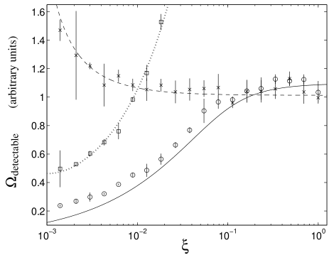
Figure 1: This plot shows the minimum gravitational-wave energy density $\Omega_{\rm detectable}$ necessary for detection, for several different detection statistics, as a function of the background’s Gaussianity parameter $\xi$. The Gaussianity parameter $\xi$ is the probability that, at any randomly chosen time, the waves from an event are incident on the detectors, and thus takes values in the interval $0\leq\xi\leq 1$. For a Gaussian background $\xi=1$. The circles are the results of our Monte Carlo simulations for the maximum likelihood statistic $\Lambda_{\text{ML}}^{\text{NG}}$, and the solid curve shows the approximate theoretical prediction (168) and (177) for this statistic (expected to be accurate only to within a few tens of percent). The crosses are the Monte Carlo results for the cross-correlation statistic $\Lambda_{\text{CC}}$, and the dashed curve shows the theoretical prediction (LABEL:analytic_detectable) for this statistic. Finally the squares are the Monte Carlo results for the burst statistic (9), and the dotted curve shows the corresponding theoretical prediction given by Eqs. (66) and (67). For each statistic, the vertical error bars on the Monte Carlo simulation results give the fluctuations computed from 4 different runs, each with 2000 trials. The number of data points is $N=10^{4}$, and the false alarm and false dismissal probabilities are both $0.1$. A detailed description of the simulations and the analytical predictions can be found in Sec. IV.

That comparison is quantified in terms of the the minimum gravitational-wave energy density $\Omega_{\text{detectable}}$ necessary for detection. The values of this quantity for the three different statistics $\Lambda_{\text{ML}}^{\text{NG}}$, $\Lambda_{\text{CC}}$ and $\Lambda_{\text{B}}$ we will denote by $\Omega_{\text{detectable}}^{\text{ML}}$, $\Omega_{\rm detectable}^{\text{CC}}$, and $\Omega_{\text{detectable}}^{\text{B}}$, respectively. Results for these three quantities obtained from Monte Carlo simulations are shown in Fig. 1, which gives $\Omega_{\text{detectable}}$ as a function of $\xi$ for $N=10^{4}$ data points. The Monte Carlo simulations are described in Sec. IV.2 below. The figure shows that in the limit $\xi\to 1$ of Gaussian signals, the statistics $\Lambda_{\text{ML}}^{\text{NG}}$ and $\Lambda_{\text{CC}}$ perform approximately equivalently (the cross-correlation statistic is slightly better). As the Gaussianity parameter $\xi$ is decreased, the performance of $\Lambda_{\text{ML}}^{\text{NG}}$ improves, until at $\xi\sim 10^{-2.5}$ it is better than that of $\Lambda_{\text{CC}}$ by about a factor of $3$ in energy density. Finally, in the limit $\xi\to 0$, the individual bursts become visible and the burst statistic $\Lambda_{\text{B}}$ becomes the best statistic.

Figure 1 also shows theoretical curves for the three quantities $\Omega_{\text{detectable}}^{\text{ML}}$, $\Omega_{\rm detectable}^{\text{CC}}$, and $\Omega_{\text{detectable}}^{\text{B}}$. These curves are derived and discussed in Sec. IV below. For the burst and cross-correlation statistics, the theoretical curves should have a fractional accuracy $\sim 1/\sqrt{N}$. For the maximum likelihood statistic, the theoretical prediction is expected to be accurate to a few tens of percent. These expected accuracies are confirmed by the Monte Carlo simulations, as seen in Fig. 1.

The value $N=10^{4}$ of the number of data points is roughly appropriate for a space based detector like LISA, for which the duration of a measurement might be $\sim 1$ year and the effective bandwidth $\sim 10^{-3}$ Hz. However, for year-long observations with ground based detectors, the effective bandwidth will be $\sim 100$ Hz and consequently the appropriate value of $N$ is $\sim 10^{9}$. We were unable to perform Monte Carlo simulations for this large value of $N$ due to limitations in available computing power. However, we show in Fig. 2 the theoretical curves for the three different statistics as functions of $\xi$ for $N=10^{9}$. In this case, the maximum likelihood statistic starts to outperform the cross-correlation statistic at $\xi\sim 10^{-3}$, and the maximum gain factor in energy density is of order $\sim 2$.

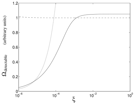
Figure 2: The minimum gravitational-wave energy density $\Omega_{\rm detectable}$ necessary for detection as a function of the background’s Gaussianity parameter $\xi$ for $N=10^{9}$ data points, which is a realistic number of data points for ground based detectors. The false alarm and false dismissal probabilities are both 0.01. The solid line is the theoretical prediction (168) and (177) for the maximum likelihood statistic, which is expected to be accurate to a few tens of percent. The dashed line is the theoretical prediction (63) for the cross correlation statistic, and the dotted line is the theoretical prediction (66)–(67) for the burst statistic; see caption to Fig. 1. This plot indicates a maximum gain factor of $\sim 2$ in energy density for duty cycles in a narrow band near $\xi\sim 10^{-4}$.

We next discuss the computational cost of the maximum likelihood statistic $\Lambda_{\rm ML}^{\rm NG}$. As is well known, the computational cost of trying to detect a stochastic background using the cross-correlation statistic $\Lambda_{\text{CC}}$ is negligible when compared to, say, matched-filter-based inspiral waveform searches. However, because of the non-trivial maximization in Eq. (8), the maximum likelihood statistic $\Lambda_{\text{ML}}^{\text{NG}}$ is computationally intensive. In fact, every evaluation of the function to be maximized over the four parameters $\xi$, $\alpha$, $\sigma_{1}$, and $\sigma_{2}$ requires computing a length-$N$ sum or product, where $N$ is the number of data points, and takes longer than the entire cross-correlation detection method. Depending on the method of calculation, the computational cost of computing $\Lambda_{\text{ML}}^{\text{NG}}$ is larger than that of computing $\Lambda_{\text{CC}}$ by a factor anywhere from $10^{2}$ to $10^{4}$.

To summarize, under the idealized assumptions of this paper, if one searches for a stochastic background using the standard cross-correlation statistic, then one might not detect a signal that would have been detectable using our maximum likelihood statistic. This conclusion probably generalizes to realistic detector noise models and detector orientations.

I.5 Outline of this paper

In Sec. II we introduce notation, review the general theory of signal detection and parameter measurement, and derive a general form of the maximum likelihood detection statistic. Then, in Sec. III, we derive the maximum likelihood statistics for both a Gaussian background (Sec. III.2) and for the model (7) of a non-Gaussian background (Sec. III.3), assuming two idealized detectors. In Sec. IV we discuss analytical calculations and Monte Carlo simulations comparing the performance of the maximum likelihood and cross-correlation detection statistics. Also in Sec. IV we show how the signal parameters $\xi$ and $\alpha$ can be estimated, with reasonable accuracy, for a strong non-Gaussian background. We conclude in Sec. V with a discussion of the results.

II General theory of detection statistics and parameter estimation

In this section we review various formal aspects of the theory of signal detection and measurement. We derive a form of the maximum likelihood detection statistic that is more general than has been considered before in the context of gravitational wave data analysis Allen Romano ; general method ; excess power ; sam joe ; sam unpublished . The material in this section can be found in a variety of texts maximum likelihood ; we include this section for completeness and to introduce notation.

II.1 Notational conventions

We use calligraphic letters $\mathcal{A,B,C,\ldots}$ to denote random variables. As described in Sec. I.2, given $D$ detectors we can assemble an $N\times D$ detector output matrix $\mathcal{H}$ with components $\mathcal{H}_{i}^{k}$ where $k=1,2,\ldots,N$ is a time index, and $i=1,2,\dots,D$ labels the detector. We assume that the detector outputs are made up of noise $\mathcal{N}$ and signal $\mathcal{S}$ with components $\mathcal{N}_{i}^{k}$ and $\mathcal{S}_{i}^{k}$ respectively, such that

$$\mathcal{H=N+S}.$$ (10)

Specific realizations of random variables will be denoted by lower case Roman symbols. For example, $h=n+s$ is a specific realization of Eq. (10), where the components of $h$ are $h_{i}^{k}$.

Probability densities for random variables will always be denoted by a lowercase $p$ and will carry a subscript to indicate which random variable is being described. For example, $p_{\mathcal{N}}(n)d^{ND}n$ is the probability that $n<\mathcal{N}<n+dn$, where $d^{ND}n$ is the product

$$d^{ND}n=\prod_{k=1}^{N}\prod_{i=1}^{D}dn_{i}^{k}.$$ (11)

We write the normalization requirement for $p_{\mathcal{N}}(n)$ as

$$1=\int d^{ND}n~{}p_{\mathcal{N}}(n).$$ (12)

Unless otherwise specified, integrals are over $\mathbb{R}^{ND}$ where $\mathbb{R}$ is the set of real numbers.

We assume a detector noise model with $Q_{n}$ parameters. Let $\mathcal{V}_{n}$ be a vector of length $Q_{n}$ whose components are the parameters characterizing the noise in the detectors. We denote by $\Theta_{n}$ the space of all possible values of $\mathcal{V}_{n}$. Here the subscript $n$ is not an index; it is merely short for “noise”. We denote joint probabilities in the usual way. For example, $p_{{\mathcal{N}},{\mathcal{V}}_{n}}(n,{\bf v}_{n})d^{ND}n~{}d^{Q_{n}}v_{n}$ is the probability that $n<\mathcal{N}<n+dn$ and ${\bf v}_{n}<\mathcal{V}_{n}<{\bf v}_{n}+d{\bf v}_{n}$, where $d^{Q_{n}}v_{n}$ is defined by

$$d^{Q_{n}}v_{n}=\prod_{l=1}^{Q_{n}}dv_{n}^{l},$$ (13)

and $dv_{n}^{l}$ is the $l$th component of $d{\bf v}_{n}$. We also use vertical bars to denote conditional probabilities. For example

$$p_{\mathcal{N|V}_{n}}(n|{\bf v}_{n})d^{ND}n=\frac{p_{\mathcal{N,V}_{n}}(n,{\bf v}_{n})d^{Q_{n}}v_{n}}{p_{\mathcal{V}_{n}}({\bf v}_{n})d^{Q_{n}}v_{n}}d^{ND}n$$ (14)

is the probability that $n<\mathcal{N}<n+dn$ given that ${\bf v}_{n}<\mathcal{V}_{n}<{\bf v}_{n}+d{\bf v}_{n}$.

We will often use the so-called total probability theorem Papoulis to write probability densities for a specific random variable as an integral over the functional dependencies of that random variable. An example is

$$p_{\mathcal{N}}(n)=\int_{\Theta_{n}}d^{Q_{n}}v_{n}~{}p_{\mathcal{N|V}_{n}}(n|{\bf v}_{n})p_{\mathcal{V}_{n}}({\bf v}_{n}).$$ (15)

Expanding probability densities in this way allows us to treat parameters, such as the noise parameters $\mathcal{V}_{n}$ in Eq. (15), as unknowns. In fact, such a treatment of the noise parameters is the crucial difference between the derivations of this work and those in previous studies of gravitational wave data analysis techniques Allen Romano ; general method ; excess power ; sam joe ; sam unpublished .

We assume that the signal model contains $Q_{s}$ parameters, which we will treat as random variables like the noise parameters. We will denote by ${\mathcal{V}}_{s}$ the random vector of length $Q_{s}$ containing the signal parameters, and by $\Theta_{s}$ the space of all possible values of ${\mathcal{V}}_{s}$.

We define the notions of “signal present” and “signal absent” in terms of a partition of the space $\Theta_{s}$ of signal parameters into a disjoint union

$$\Theta_{s}=\Theta_{s0}\cup\Theta_{s1},$$ (16)

where $\Theta_{s0}$ corresponds to the signal being absent, and $\Theta_{s1}$ the signal being present. We define the random variable $\mathcal{T}$, taking values $\mathcal{T}=0$ or $\mathcal{T}=1$, according to

$$\mathcal{T}=\left\{\begin{array}[]{ll}1&\text{ if }\mathcal{V}_{s}\in\Theta_{s1}\\ 0&\text{ if }\mathcal{V}_{s}\in\Theta_{s0}\end{array}\right..$$ (17)

Thus $\mathcal{T}=1$ corresponds to a signal being present, and $\mathcal{T}=0$ to no signal being present. We define

$$p_{\mathcal{S|V}_{s},\mathcal{T}}(s|{\bf v}_{s},0)=\left\{\begin{array}[]{ll}0&\text{ if }{\bf v}_{s}\in\Theta_{s1}\\ \delta^{ND}(s)&\text{ if }{\bf v}_{s}\in\Theta_{s0}\end{array}\right.,$$ (18)

where $\delta^{ND}(s)$ is the $N\times D$ dimensional Dirac delta function. We denote by $p_{\mathcal{T,H}}(t,h)d^{ND}h$ the probability that $\mathcal{T}=t$ and that $h<\mathcal{H}<h+dh$, where $t=0$ or $1$. Similarly

$$p_{\mathcal{H|T}}(h|t)d^{ND}h=\frac{p_{\mathcal{H,T}}(h,t)}{P_{\mathcal{T}}(t)}d^{ND}h$$ (19)

is the probability that $h<\mathcal{H}<h+dh$ given that $\mathcal{T}=t$.

We denote probabilities (as opposed to probability densities) with an uppercase $P$. For example $P_{\mathcal{T}}(1)$ is the probability that a signal is present, and $P_{\mathcal{T}}(0)$ is the probability that a signal is absent.

Before examining the detector outputs, we may have some idea, say from previous experiments, of the probability that a signal will be present. We denote this prior probability by $P^{(0)}$. We denote by $P^{(1)}$ the posterior probability that the signal is present after examining $\mathcal{H}$ in the context of all prior experiments etc. All posterior quantities have an implicit dependence on the detector outputs. To simplify the notation we will not explicitly show this dependence. For example, we write $P^{(1)}$ rather than the more cumbersome $P^{(1)}(\mathcal{H})$ for the posterior probability that a signal is present.

There are prior and posterior versions of all probability densities. When necessary we will append superscripts of $(0)$ and $(1)$ to distinguish priors and posteriors respectively. For example $p^{(1)}_{\mathcal{V}_{n}}({\bf v}_{n})=p_{\mathcal{V}_{n}|\mathcal{H}}({\bf v}_{n}|h)$ is the posterior probability density for $\mathcal{V}_{n}$. The posterior distribution for the noise can be expanded in terms of $p^{(1)}_{\mathcal{V}_{n}}({\bf v}_{n})$ as

$$p^{(1)}_{\mathcal{N}}(n)=\int_{\Theta_{n}}d^{Q_{n}}v_{n}~{}p_{\mathcal{N|V}_{n}}(n|{\bf v}_{n})p^{(1)}_{\mathcal{V}_{n}}({\bf v}_{n}).$$ (20)

The conventions and symbols which have been introduced above are summarized in tables 1 and 2 respectively.

Table 1: A summary of conventions introduced in Sec. II.1.

Convention	Example
Random variables are denoted by upper case calligraphic letters.	The detector output matrix is denoted by $\mathcal{H}$.
Specific realizations of random variables are denoted by lower case Roman letters. (see next convention)	A specific observation run may result in a specific detector output matrix $h$ or say $x$. These results would be denoted $\mathcal{H}=h$ and $\mathcal{H}=x$ respectively.
A lower case $p$ denotes a probability density function (PDF). It’s subscript determines the quantities with which it is associated.	The PDF for the detector output $\mathcal{H}$ as a function of $h$, or say $x$, is denoted by $p_{\mathcal{H}}(h)$ and $p_{\mathcal{H}}(x)$ respectively.
A comma in a PDF subscript and argument indicates a joint PDF.	The joint PDF for $\mathcal{N}$ and $\mathcal{V}_{n}$ as a function of $n$ and ${\bf v}_{n}$ respectively is denoted by $p_{\mathcal{N},\mathcal{V}_{n}}(n,{\bf v}_{n})$.
A vertical bar in a PDF subscript and argument indicates a conditional PDF.	The conditional PDF for $\mathcal{N}$ and $\mathcal{V}_{n}$ as a function of $n$ and ${\bf v}_{n}$ respectively is denoted by $p_{\mathcal{N}|\mathcal{V}_{n}}(n|{\bf v}_{n})$.
An upper case $P$ denotes a probability.	The probability that $\mathcal{T}=1$ is denoted by $P_{\mathcal{T}}(1)$.
Prior and posterior quantities are denoted by superscripts of $(0)$ and $(1)$ respectively.	The prior probability that a signal is present is denoted by $P^{(0)}$, while the posterior probability that a signal is present, after an observation $\mathcal{H}=h$, is denoted by $P^{(1)}=P_{\mathcal{T}|\mathcal{H}}(1|h)$.

Table 2: A summary of symbols introduced in Sec. II.1.

Symbol	Meaning
$\mathcal{H},h$	detector output matrix
$\mathcal{N},n$	noise contribution to detector output matrix
$\mathcal{S},s$	signal contribution to detector output matrix
$N$	number of strain samples taken from one detector
$D$	number of detectors
$Q_{n}$	number of parameters in the model noise PDF
$Q_{s}$	number of parameters in the model signal PDF
$\mathcal{V}_{n},{\bf v}_{n}$	the parameters of the model noise PDF
$\mathcal{V}_{s},{\bf v}_{s}$	the parameters of the model signal PDF
$\Theta_{n}$	the space of all possible values of $\mathcal{V}_{n}$
$\Theta_{s}$	the space of all possible values of $\mathcal{V}_{s}$
$\Theta_{s0}$	the subspace of $\Theta_{s}$ for which a signal is absent
$\Theta_{s1}$	the subspace of $\Theta_{s}$ for which a signal is present
$\mathcal{T},t$	1 if a signal is present ($\mathcal{V}_{s}\in\Theta_{s1}$), otherwise 0
$P^{(0)}$	prior probability that a signal is present
$P^{(1)}$	posterior probability that a signal is present

II.2 Detection statistics

To detect a signal one uses a detection statistic, say $\Gamma=\Gamma(\mathcal{H})$, that is some function of the detector outputs ${\cal H}$. A signal is said to have been detected when $\Gamma$ exceeds some threshold value $\Gamma_{*}$.

Denote by $P_{\text{FD}}(\Gamma_{*})$ the probability of false dismissal, that is, the probability that we fail to detect a signal which is actually present. Similarly, let $P_{\text{FA}}(\Gamma_{*})$ be the probability that we claim to have detected a signal which in fact is absent—the probability of false alarm. For given signal and noise models and for a given statistic $\Gamma$, the false alarm and false dismissal probabilities generate a curve in the $P_{\text{FA}}$-$P_{\text{FD}}$ plane parametrized by the threshold $\Gamma_{*}$. Such curves depend on the number of detectors $D$, the number of data points $N$, the signal parameters $\mathcal{V}_{s}$, and the noise parameters $\mathcal{V}_{n}$.

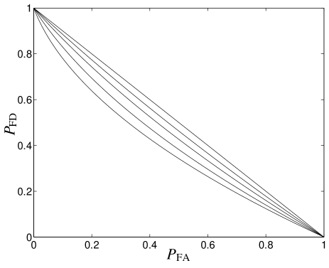
Figure 3: False dismissal versus false alarm curves for typical detection statistics.

Suppose that the statistic $\Gamma$ is bounded in the sense that there exist numbers $\Gamma_{\min}$ and $\Gamma_{\max}$ such that $\Gamma_{\min}<\Gamma<\Gamma_{\max}$ for all ${\cal H}$. Then it is clear that $P_{\text{FD}}(\Gamma_{\min})=0$ and that $P_{\text{FA}}(\Gamma_{\min})=1$. As the threshold $\Gamma_{*}$ increases toward $\Gamma_{\max}$, $P_{\text{FD}}(\Gamma_{*})$ will increase while $P_{\text{FA}}(\Gamma_{*})$ decreases, until finally at $\Gamma_{*}=\Gamma_{\rm max}$, $P_{\text{FD}}=1$, and $P_{\text{FA}}=0$. Thus, false dismissal-false alarm curves generally look something like those sketched in Fig. 3.

Note that if one uses a different statistic $f(\Gamma)$, where $f$ is any function, then the shape of the $P_{\text{FA}}$-$P_{\text{FD}}$ curve does not change as long as $f$ is monotonic in the sense that

$$\Gamma>\Gamma_{*}~{}\Rightarrow~{}f(\Gamma)>f(\Gamma_{*}).$$ (21)

Only the parametrization of the curve changes under such a transformation. Statistics related by transformations $f$ satisfying the monotonicity property (21) have identical false dismissal versus false alarm curves.

In 1933 Neyman and Pearson considered a simple signal detection scenario where the sets $\Theta_{n}$, $\Theta_{s1}$, and $\Theta_{s0}$ each contain a single element Neyman and Pearson . They showed that for this scenario the detection statistic which minimizes $P_{\text{FD}}$ for any $P_{\text{FA}}$ is the so-called likelihood ratio $\Lambda$, defined by

$$\Lambda=\frac{p_{\mathcal{H|T}}(h|1)}{p_{\mathcal{H|T}}(h|0)}.$$ (22)

One notion of optimality for detection statistics is that the statistic should minimize the false dismissal probability at a fixed value of the false alarm probability. For the simple scenario above, this criteria, known as the Neyman-Pearson criteria, uniquely determines the likelihood ratio as the optimal statistic Ferguson . However in general, when any of $\Theta_{n}$, $\Theta_{s1}$, or $\Theta_{s0}$ contains more than one element, the statistic selected by this criteria is a function of the unknown parameters $\mathcal{V}_{s}$ and $\mathcal{V}_{n}$. Thus, as is well known, the Neyman-Pearson criteria does not single out a unique statistic in such cases.

In this paper we will obtain our detection statistics from Bayesian considerations, but we will quantify their effectiveness using the Neyman and Pearson criteria of comparing false dismissal probabilities at fixed false alarm probabilities.

II.3 Likelihood ratio and likelihood function

From a Bayesian point of view, a natural criterion for deciding that a signal is present is for the posterior probability $P^{(1)}$ to exceed some threshold Bayes . The posterior probability $P^{(1)}$ is related to the prior probability $P^{(0)}$ and to the likelihood ratio $\Lambda$ defined by Eq. (22) by

$$\frac{P^{(1)}}{1-P^{(1)}}=\Lambda\frac{P^{(0)}}{1-P^{(0)}}.$$ (23)

See appendix A for a derivation of Eq. (23) in the most general context where the sets $\Theta_{n}$, $\Theta_{s1}$, and $\Theta_{s0}$ are all non-trivial. It follows from Eq. (23) that $P^{(1)}$ is a monotonic function of $\Lambda$, so thresholding on $P^{(1)}$ is equivalent to thresholding on $\Lambda$. This makes $\Lambda$, or approximate versions of it, the natural choice for a detection statistic.

We derive in Appendix A the following general formula for the likelihood ratio as a function of the data ${\cal H}=h$:

$$\Lambda=\frac{\displaystyle\int_{\Theta_{s1}}d^{Q_{s}}v_{s}~{}\int d^{ND}s~{}\int_{\Theta_{n}}d^{Q_{n}}v_{n}~{}p_{\mathcal{N|V}_{n}}(h-s|{\bf v}_{n})p_{\mathcal{V}_{n}}({\bf v}_{n})p_{\mathcal{S|V}_{s},\mathcal{T}}(s|{\bf v}_{s},1)p_{\mathcal{V}_{s}|\mathcal{T}}({\bf v}_{s}|1)}{\displaystyle\int_{\Theta_{n}}d^{Q_{n}}v_{n}^{\prime}~{}p_{\mathcal{N|V}_{n}}(h|{\bf v}_{n}^{\prime})p_{\mathcal{V}_{n}}({\bf v}_{n}^{\prime})}.$$ (24)

The various probability distributions that appear in Eq. (24) are (i) the prior distribution $p_{\mathcal{V}_{s}|\mathcal{T}}({\bf v}_{s}|1)$ for the signal parameters ${\bf v}_{s}$; (ii) the distribution $p_{\mathcal{S|V}_{s},\mathcal{T}}(s|{\bf v}_{s},1)$ for the signal $s$ given the signal parameters ${\bf v}_{s}$; (iii) the prior distribution $p_{\mathcal{V}_{n}}({\bf v}_{n})$ for the noise parameters ${\bf v}_{n}$; and (iv) the distribution $p_{\mathcal{N|V}_{n}}(h|{\bf v}_{n})$ for the noise $n$ given the noise parameters ${\bf v}_{n}$.

We can interpret Eq. (24) as follows. In the simple signal detection scenario, we choose between a pair of simple claims: (i) $\mathcal{V}_{s}={\bf v}_{s0}$ or (ii) $\mathcal{V}_{s}={\bf v}_{s1}$. In general we choose between a pair of complicated, or composite, claims: (i) $\mathcal{V}_{s}\in\Theta_{s0}$ or (ii) $\mathcal{V}_{s}\in\Theta_{s1}$, where both $\Theta_{s0}$ and $\Theta_{s1}$ contain many elements. Equation (24) says that the best way to chose between a pair of complicated claims is to first break the complicated pair of claims into pairs of simple claims, then compute the likelihood ratio for each pair of simple claims, and sum the results of each choice. That is, the likelihood ratio can be written as an integral over the parameters of the composite claims

$$\Lambda=\int_{\Theta_{s1}}d^{Q_{s}}v_{s}~{}\int_{\Theta_{n}}d^{Q_{n}}v_{n}~{}\Lambda({\bf v}_{s},{\bf v}_{n}),$$ (25)

where the integrand $\Lambda({\bf v}_{s},{\bf v}_{n})$, which we refer to as the likelihood function, can be read off from Eq. (24):

$$\Lambda({\bf v}_{s},{\bf v}_{n})=\frac{\displaystyle\int d^{ND}s~{}p_{\mathcal{N|V}_{n}}(h-s|{\bf v}_{n})p_{\mathcal{S|V}_{s},\mathcal{T}}(s|{\bf v}_{s},1)p_{\mathcal{V}_{n}}({\bf v}_{n})p_{\mathcal{V}_{s}|\mathcal{T}}({\bf v}_{s},1)}{\displaystyle\int_{\Theta_{n}}d^{Q_{n}}v_{n}^{\prime}~{}p_{\mathcal{N|V}_{n}}(h|{\bf v}_{n}^{\prime})p_{\mathcal{V}_{n}}({\bf v}_{n}^{\prime})}.$$ (26)

The likelihood function $\Lambda({\bf v}_{s},{\bf v}_{n})$ can be used to compute the posterior probability density $p^{(1)}_{\mathcal{V}_{s},\mathcal{V}_{n}|\mathcal{T}}({\bf v}_{s},{\bf v}_{n}|1)$ for the signal and noise parameters given that a signal is present, via the formula

$$\frac{P^{(1)}}{1-P^{(1)}}p^{(1)}_{\mathcal{V}_{s},\mathcal{V}_{n}|\mathcal{T}}({\bf v}_{s},{\bf v}_{n}|1)=\Lambda({\bf v}_{s},{\bf v}_{n})\frac{P^{(0)}}{1-P^{(0)}}.$$ (27)

A derivation of Eq. (27) can be found in appendix A.

II.4 Maximum likelihood detection statistics and parameter estimators

In many applications, it is impractical to compute the detection statistic (24) because of the multi-dimensional integrals involved Loredo . However, approximate versions of the statistic are often easier to compute and useful. If a signal is present with sufficiently large amplitude, then the integrand in the numerator of Eq. (24) will be sharply peaked. The integrand in the denominator of Eq. (24) will also be sharply peaked when there is sufficient data that the noise is well characterized. Under these circumstances, the integrals can be written as the values of the corresponding integrands at the peaks multiplied by “width factors”, where the width factors depend only weakly on the data $h$ and can be neglected without affecting much the performance of the statistic. [The width factors from the integrals over the noise parameters will tend to cancel between the numerator and denominator]. Also, frequently the prior distributions for $\mathcal{V}_{s}$ and $\mathcal{V}_{n}$ are slowly varying, and neglecting those distributions has a negligible effect on the performance of the statistic. Under these conditions the maximum likelihood detection statistic $\Lambda_{\text{ML}}$ defined by

$$\Lambda_{\text{ML}}=\frac{\displaystyle\max_{{\bf v}_{s}\in\Theta_{s1}}~{}\max_{{\bf v}_{n}\in\Theta_{n}}~{}\int d^{ND}s~{}p_{\mathcal{N|V}_{n}}(h-s|{\bf v}_{n})p_{\mathcal{S|V}_{s},\mathcal{T}}(s|{\bf v}_{s},1)}{\displaystyle\max_{{\bf v^{\prime}}\in\Theta_{n}}~{}p_{\mathcal{N|V}_{n}}(h|{\bf v}_{n}^{\prime})}$$ (28)

is a natural approximate version of $\Lambda$ . The subscript ML denotes that (28) is the maximum likelihood approximate version of $\Lambda$. See Ref. maximum likelihood for further discussion of $\Lambda_{\text{ML}}$ as an approximate version of $\Lambda$ .

A particular special case of the detection statistic (28), which is widely used, is the following. Assume that the noise parameters have some known values $\mathcal{V}_{n}={\bf v}_{n}$. Then the noise priors and the $\Theta_{n}$ integrals in Eq. (24) are trivial, and one obtains the detection statistic

$$\tilde{\Lambda}_{\text{ML}}=\frac{\displaystyle\max_{{\bf v}_{s}\in\Theta_{s1}}~{}\int d^{ND}s~{}p_{\mathcal{N|V}_{n}}(h-s|{\bf v}_{n})p_{\mathcal{S|V}_{s},\mathcal{T}}(s|{\bf v}_{s},1)}{\displaystyle p_{\mathcal{N|V}_{n}}(h|{\bf v}_{n})}.$$ (29)

See Ref. sam joe for an exploration of the statistic (29) in the context of stochastic backgrounds. We will show below that for a Gaussian stochastic background, $\Lambda_{\text{ML}}$ reduces to the standard cross-correlation statistic while the more specialized statistic $\tilde{\Lambda}_{\text{ML}}$ does not. Thus for stochastic backgrounds, treating the noise parameters as unknowns is crucial robust gaussian II .

When the noise and signal parameters $\mathcal{V}_{n}$ and $\mathcal{V}_{s}$ can take on many values, one naturally would like to know which values are realized. Equation (27) suggests using the values $\hat{\bf v}_{n}$ and $\hat{\bf v}_{s}$ defined by

$$\Lambda(\hat{\bf v}_{s},\hat{\bf v}_{n})=\max_{{\bf v}_{s}\in\Theta_{s1}}~{}\max_{{\bf v}_{n}\in\Theta_{n}}~{}\Lambda({\bf v}_{s},{\bf v}_{n}).$$ (30)

The estimators $\hat{\bf v}_{n}$ and $\hat{\bf v}_{s}$ are known as maximum likelihood estimators. Note that ${\bf v}_{s}=\hat{\bf v}_{s}$ and ${\bf v}_{n}=\hat{\bf v}_{n}$ also maximize the numerator in Eq. (28). For the remainder of this paper we will use $\Lambda_{\text{ML}}$, defined by Eq. (28), as our detection statistic, and $\hat{\bf v}_{s}$ and $\hat{\bf v}_{n}$, defined by Eq. (30), as parameter estimators.

III Application to stochastic background searches

In this section we derive the maximum likelihood detection statistic (28) for a simplified model of the detection problem for stochastic gravitational waves, and for a specific simple model of a non-Gaussian stochastic background.

III.1 Assumptions

We assume two detectors with outputs $\mathcal{H}_{i}^{k}$, where $i=1,2$ labels the detector and $k=1,2,\ldots,N$ is a time index. We assume that the noise in detector one is uncorrelated with the noise in detector two. We will require the noise in both detectors to have vanishing mean and to be both Gaussian and white, so that

$$p_{\mathcal{N|V}_{n}}\left[n|(\sigma_{1},\sigma_{2})\right]=\prod_{k=1}^{N}\frac{1}{2\pi\sigma_{1}\sigma_{2}}\exp\left[-\frac{(n_{1}^{k})^{2}}{2\sigma^{2}_{1}}-\frac{(n_{2}^{k})^{2}}{2\sigma^{2}_{2}}\right].$$ (31)

The parameters $\sigma_{1}$ and $\sigma_{2}$ in Eq. (31) are the square roots of the variances of the noise in the two detectors. For this model ${\bf v}_{n}=(\sigma_{1},\sigma_{2})$ and $\Theta_{n}=\left\{(\sigma_{1},\sigma_{2})~{}|~{}\sigma_{1}\geq 0\text{ and }\sigma_{2}\geq 0\right\}$.

We assume that the detectors are collocated and aligned, so that the same signal is present in both detectors

$$\mathcal{S}_{1}^{k}=\mathcal{S}_{2}^{k}=\mathcal{S}^{k}.$$ (32)

Lastly we assume that the individual signal samples are uncorrelated and identically distributed, i.e., the signal is white, so that

$$p_{\mathcal{S}}(s)=\prod_{k=1}^{N}p_{\mathcal{S}^{k}}(s^{k}).$$ (33)

Our assumptions (31)-(33) are unrealistic for both ground-based and space-based detectors: we expect the noise to be colored with significant non-Guasssian components, and in general detectors will not be co-located and aligned. Our analysis is therefore just a first step, and will need to be generalized. However, we expect that our central conclusion — the existence of statistics which outperform the standard cross-correlation statistic for nonGaussian signals — is robust, and will not be altered when these complications are taken into account.

We now derive a general formula for the maximum likelihood statistic (28), which we apply in both the Gaussian and non-Gaussian cases in the following two subsections. The denominator in Eq. (28) can be written, from Eq. (31), as

$$\max_{\sigma_{1}\geq 0}~{}\max_{\sigma_{2}\geq 0}~{}\left\{\left(2\pi\sigma_{1}\sigma_{2}\right)^{-N}\exp\left[-\frac{N}{2}\left(\frac{\bar{\sigma}^{2}_{1}}{\sigma^{2}_{1}}+\frac{\bar{\sigma}^{2}_{2}}{\sigma^{2}_{2}}\right)\right]\right\},$$ (34)

where $\bar{\sigma}_{1}^{2}$ and $\bar{\sigma}_{2}^{2}$ are defined by

$$\bar{\sigma}^{2}_{i}=\frac{1}{N}\sum_{k=1}^{N}\left(h_{i}^{k}\right)^{2}$$ (35)

for $i=1,2$. It is easily shown that the maximum in Eq. (34) is achieved at $\sigma_{i}=\bar{\sigma}_{i}$. From Eq. (28) this yields

$$\Lambda_{\text{ML}}=\frac{\displaystyle\max_{{\bf v}_{s}\in\Theta_{s1}}~{}\max_{{\bf v}_{n}\in\Theta_{n}}~{}\int d^{ND}s~{}p_{\mathcal{N|V}_{n}}(h-s|{\bf v}_{n})p_{\mathcal{S|V}_{s},\mathcal{T}}(s|{\bf v}_{s},1)}{\displaystyle\left(2\pi\bar{\sigma}_{1}\bar{\sigma}_{2}\right)^{-N}\exp\left(-N\right)}.$$ (36)

Combining this with Eq. (33) yields the following final general expression for the maximum likelihood statistic:

$$\Lambda_{\text{ML}}=\max_{{\bf v}_{s}\in\Theta_{s1}}~{}\max_{\sigma_{1}\geq 0}~{}\max_{\sigma_{2}\geq 0}~{}\prod_{k=1}^{N}\frac{\bar{\sigma}_{1}\bar{\sigma}_{2}}{\sigma_{1}\sigma_{2}}\int_{-\infty}^{\infty}ds^{k}~{}p_{\mathcal{S}^{k}|\mathcal{V}_{s},\mathcal{T}}(s^{k}|{\bf v}_{s},1)\exp\left[-\frac{\left(h_{1}^{k}-s^{k}\right)^{2}}{2\sigma^{2}_{1}}-\frac{\left(h_{2}^{k}-s^{k}\right)^{2}}{2\sigma^{2}_{2}}+1\right].$$ (37)

III.2 Gaussian signal

We now consider the case where the signal is Gaussian and has a vanishing mean. We denote by $\alpha^{2}$ the variance of the signal, so the prior for $\mathcal{S}$ is given by

$$p_{\mathcal{S}^{k}|\mathcal{V}_{s},\mathcal{T}}(s^{k}|\alpha,1)=\frac{1}{\sqrt{2\pi}\alpha}\exp\left[-\frac{\left(s^{k}\right)^{2}}{2\alpha^{2}}\right].$$ (38)

For this model ${\bf v}_{s}=(\alpha)$ has only one component, and $\Theta_{s1}=\{\alpha~{}|~{}\alpha>0\}$.

Substituting the signal probability distribution (38) into the general expression (37) for $\Lambda_{\text{ML}}$ yields a Gaussian integral which is straightforward to evaluate. The result is

$$\Lambda^{\text{G}}_{\text{ML}} = \max_{\alpha>0}~{}\max_{\sigma_{1}\geq 0}~{}\max_{\sigma_{2}\geq 0}\left\{\frac{\bar{\sigma}_{1}\bar{\sigma}_{2}}{\sqrt{\sigma_{1}^{2}\sigma_{2}^{2}+\sigma_{1}^{2}\alpha^{2}+\sigma_{2}^{2}\alpha^{2}}}\right.$$

$$\times \left.\exp\left[\frac{\frac{\bar{\sigma}_{1}^{2}}{\sigma_{1}^{4}}+\frac{\bar{\sigma}_{2}^{2}}{\sigma_{2}^{4}}+\frac{2\bar{\alpha}^{2}}{\sigma_{1}^{2}\sigma_{2}^{2}}}{2\left(\frac{1}{\sigma_{1}^{2}}+\frac{1}{\sigma_{2}^{2}}+\frac{1}{\alpha^{2}}\right)}-\frac{\bar{\sigma}_{1}^{2}}{2\sigma_{1}^{2}}-\frac{\bar{\sigma}_{2}^{2}}{2\sigma_{2}^{2}}+1\right]\right\}^{N},$$

where

$$\bar{\alpha}^{2}=\frac{1}{N}\sum_{k=1}^{N}h_{1}^{k}h_{2}^{k},$$ (40)

and we have appended a superscript G on $\Lambda^{\text{G}}_{\text{ML}}$ to indicate the maximum likelihood detection statistic for a Gaussian signal.

One can show that the maximum in Eq. (III.2) is achieved at $\alpha=\hat{\alpha}$, $\sigma_{1}=\hat{\sigma}_{1}$, and $\sigma_{2}=\hat{\sigma}_{2}$, where

$$\hat{\alpha}^{2} = \bar{\alpha}^{2}~{}\theta(\bar{\alpha}^{2}),$$ (41)

$$\hat{\sigma}^{2}_{i} = (\bar{\sigma}^{2}_{i}-\hat{\alpha}^{2})~{}\theta\left(\bar{\sigma}^{2}_{i}-\hat{\alpha}^{2}\right),$$ (42)

for $i=1,2$, and $\bar{\sigma}_{1}$ and $\bar{\sigma}_{2}$ are given by Eq. (35). Here $\theta(x)$ is the step function (5). The quantities (41) and (42) are the maximum likelihood estimators for the variance $\alpha^{2}$ of the signal and the variances $\sigma_{1}^{2}$ and $\sigma_{2}^{2}$ of the noise in the two detectors. The step functions in Eqs. (41) and (42) arise as a result of the bounds of the maximization in Eq. (37).

The corresponding detection statistic is, from Eq. (III.2) ,

$$\Lambda^{\text{G}}_{\text{ML}}=\left[1-\frac{\hat{\alpha}^{4}}{\bar{\sigma}_{1}^{2}\bar{\sigma}_{2}^{2}}\right]^{-N/2}.$$ (43)

The cross-correlation statistic $\Lambda_{\text{CC}}$ can be obtained from $\Lambda_{\text{ML}}^{\text{G}}$ via a monotonic transformation which preserves false dismissal versus false alarm curves [cf. Eq. (21) above]:

$$\Lambda_{\text{CC}} = \sqrt{1-(\Lambda^{\text{G}}_{\text{ML}})^{-2/N}}$$ (44)

$$= \frac{\hat{\alpha}^{2}}{\bar{\sigma}_{1}\bar{\sigma}_{2}}.$$

Note that if we had assumed the noise parameters ${\bf v}_{n}=(\sigma_{1},\sigma_{2})$ were known, and derived a statistic from Eq. (29) rather than Eq. (28), we would have found instead the detection statistic $\tilde{\Lambda}_{\text{ML}}^{\text{G}}=\bar{\Lambda}_{\text{ML}}^{\text{G}}~{}\theta(\bar{\Lambda}_{\text{ML}}^{\text{G}})$, where

$$\bar{\Lambda}_{\text{ML}}^{\text{G}}=\bar{\alpha}^{2}+\frac{1}{2}\left[\frac{\sigma_{2}^{2}}{\sigma_{1}^{2}}(\bar{\sigma}_{1}^{2}-\sigma_{1}^{2})+\frac{\sigma_{1}^{2}}{\sigma_{2}^{2}}(\bar{\sigma}_{2}^{2}-\sigma_{2}^{2})\right],$$ (45)

which is different from the standard cross-correlation statistic. This non-standard result is obtained because of the unrealistic assumption that the noise parameters ${\bf v}_{n}=(\sigma_{1},\sigma_{2})$ are known. Different derivations of the result (45) can be found in Refs. sam joe ; robust gaussian II .

It is often useful to characterize the “strength” of a stochastic background in terms of the signal-to-noise ratio of the cross-correlation statistic (44), which we now define. First note that for large $N$, the fractional fluctuations in $\hat{\alpha}^{2}$ will be much larger than those in $\bar{\sigma}_{1}\bar{\sigma}_{2}$ . For the purpose of defining the signal-to-noise ratio, we assume that $N$ is large enough that $\bar{\sigma}_{1}$ and $\bar{\sigma}_{2}$ in Eq. (44) can be taken to be independent of $h$, so that $\Lambda_{\text{CC}}$ and $\hat{\alpha}^{2}$ are equivalent detection statistics. We also use ${\bar{\alpha}}^{2}$ instead of ${\hat{\alpha}}^{2}$ in the computations that follow, as is conventional when defining signal-to-noise ratios. If a signal is present, then the expected value of $\bar{\alpha}^{2}$ is, from Eqs. (10), (31)–(33), (38) and (40),

$$\left<\bar{\alpha}^{2}\right>=\alpha^{2}.$$ (46)

If no signal is present, so that $\alpha^{2}=0$, then the fluctuations in $\bar{\alpha}^{2}$ are given by

$$\Delta\left(\bar{\alpha}^{2}\right)=\frac{\sigma_{1}\sigma_{2}}{\sqrt{N}}.$$ (47)

The signal-to-noise ratio $\rho$ is defined to be the ratio of these two quantities:

$$\rho=\frac{\alpha^{2}\sqrt{N}}{\sigma_{1}\sigma_{2}}.$$ (48)

III.3 Non-Gaussian signal

As mentioned in the introduction, the traditional assumption that a gravitational wave stochastic background will be Gaussian requires the individual events to be sufficiently frequent and uncorrelated. Our model for a non-Gaussian signal assumes instead that the events are infrequent.

Consider a collection of similar events generating a stochastic background $\mathcal{S}$. Let $\xi$ be the probability that, at any randomly chosen time, the waves from an event are arriving at the detectors. We assume that the time structure of individual events cannot be resolved by the detectors. That is, we assume that the events occur over timescales smaller than the detectors’ resolution time, as illustrated in Fig. 4.

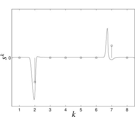
Figure 4: Sketched segment of the signal produced by a model non-Gaussian stochastic background of events unresolved by the detectors. Here we show two events. The solid curve is the exact signal. This exact signal’s contributions to the detector outputs, shown as stemmed o’s, are averages of the exact signal over the detector resolution timescale.

We assume that the distribution of the amplitudes of the events is Gaussian with variance $\alpha^{2}$. The probability distribution for the signal given the signal parameters $(\xi,\alpha)$ is therefore given by

$$p_{\mathcal{S}^{k}|\mathcal{V}_{s},\mathcal{T}}[s^{k}|(\xi,\alpha),1] = \frac{\xi}{\sqrt{2\pi}\alpha}\exp\left[-\frac{\left(s^{k}\right)^{2}}{2\alpha^{2}}\right]$$ (49)

$$+ (1-\xi)\delta\left(s^{k}\right),$$

together with Eq. (33). Thus the signal model parameters are ${\bf v}_{s}=(\xi,\alpha)$, which give respectively the “event probability” and “event variance” characterizing the stochastic background. The parameter space $\Theta_{s}$ for this model is

$$\Theta_{s}=\left\{(\xi,\alpha)~{}|~{}0\leq\xi\leq 1\text{ and }\alpha\geq 0\right\},$$ (50)

and the subset corresponding to a signal being present is

$$\Theta_{s1}=\left\{(\xi,\alpha)~{}|~{}0<\xi\leq 1\text{ and }\alpha>0\right\}.$$ (51)

Note that our assumption that the time structure of events is not resolved by the detector is unrealistic. Detector resolution times can be as small as 0.1 ms in the case of ground-based detectors like LIGO , and even supernova bursts are expected to have time scales $\gtrsim 10$ ms waveform catalog ; new waveform catalog . It will be important for future studies to relax this assumption.

We now compute the maximum likelihood detection statistic $\Lambda^{\text{NG}}_{\text{ML}}$ for our simple non-Gaussian signal model by substituting Eq. (49) into Eq. (37). This yields

$$\Lambda_{\text{ML}}^{\text{NG}} = \max_{0<\xi\leq 1}~{}\max_{\alpha>0}~{}\max_{\sigma_{1}\geq 0}~{}\max_{\sigma_{2}\geq 0}~{}\prod_{k=1}^{N}\left\{\frac{\bar{\sigma}_{1}\bar{\sigma}_{2}\xi}{\sqrt{\sigma^{2}_{1}\sigma^{2}_{2}+\sigma^{2}_{1}\alpha^{2}+\sigma^{2}_{2}\alpha^{2}}}\exp\left[\frac{\left(\frac{h_{1}^{k}}{\sigma^{2}_{1}}+\frac{h_{2}^{k}}{\sigma^{2}_{2}}\right)^{2}}{2\left(\frac{1}{\sigma^{2}_{1}}+\frac{1}{\sigma^{2}_{2}}+\frac{1}{\alpha^{2}}\right)}-\frac{\left(h_{1}^{k}\right)^{2}}{2\sigma^{2}_{1}}-\frac{\left(h_{2}^{k}\right)^{2}}{2\sigma^{2}_{2}}+1\right]\right.$$ (52)

$$+ \left.\frac{\bar{\sigma}_{1}\bar{\sigma}_{2}}{\sigma_{1}\sigma_{2}}(1-\xi)\exp\left[-\frac{\left(h_{1}^{k}\right)^{2}}{2\sigma^{2}_{1}}-\frac{\left(h_{2}^{k}\right)^{2}}{2\sigma^{2}_{2}}+1\right]\right\}.$$

The values of $\xi$, $\alpha^{2}$, $\sigma_{1}^{2}$, and $\sigma_{2}^{2}$ which achieve the maximum in Eq. (52) are, respectively, estimators of the signal’s Gaussianity parameter, the variance of the signal events, and the noise variances in the two detectors. Note that if we evaluate Eq. (52) at $\xi=1$, rather than maximizing over $\xi$, we recover Eq. (III.2) and the statistic $\Lambda_{\text{ML}}^{\text{G}}$.

We mention in passing an approximate version of the statistic (52) which is significantly easier to compute. Expanding the logarithm of the quantity to be maximized in Eq. (52) as a power series in $\alpha^{2}$ to fourth order about $\alpha^{2}=0$ yields the approximate statistic $\hat{\Lambda}_{\text{ML}}^{\text{NG}}$ given by

$$\ln\hat{\Lambda}_{\text{ML}}^{\text{NG}} = \max_{0<\xi\leq 1}~{}\max_{\alpha>0}~{}\max_{\sigma_{1}\geq 0}~{}\max_{\sigma_{2}\geq 0}~{}\sum_{n=0}^{4}\sum_{l=0}^{8}\sum_{m=0}^{8}\left(\frac{\alpha^{2}}{\sigma_{1}\sigma_{2}}\right)^{n}$$ (53)

$$\times C_{nlm}\left(\xi,\sigma_{1},\sigma_{2}\right)\sum_{k=1}^{N}(h_{1}^{k})^{l}(h_{2}^{k})^{m},$$

where the coefficients $C_{nlm}(\xi,\sigma_{1}^{2},\sigma_{2}^{2})$ vanish unless $l+m$ is even and $l+m\leq 8$. In evaluating the statistic (53), one can first evaluate the 24 sums

$$\sum_{k=1}^{N}(h_{1}^{k})^{l}(h_{2}^{k})^{m}$$ (54)

for the required values of $l$ and $m$, and subsequently numerically maximize over the parameters $\xi$, $\alpha$, $\sigma_{1}$, and $\sigma_{2}$. Thus the length-$N$ sums need only be performed once, rather than each time one tries a new set of values for $\xi$, $\alpha$, $\sigma_{1}$, and $\sigma_{2}$. Therefore the computational cost of $\hat{\Lambda}_{\text{ML}}^{\text{NG}}$ is only about an order of magnitude greater than that of the cross correlation statistic $\Lambda_{\text{CC}}$, and this statistic may be useful to explore.

We now derive the signal-to-noise ratio $\rho$ for the cross-correlation statistic and for the non-Gaussian signal (49). If the signal is present, then from Eqs. (10), (33), (40), (41) and (49) the expected value of $\bar{\alpha}^{2}$ is

$$\left<\bar{\alpha}^{2}\right>=\xi\alpha^{2}.$$ (55)

If no signal is present then the fluctuations in $\bar{\alpha}^{2}$ are given by

$$\Delta\left(\bar{\alpha}^{2}\right)=\frac{\sigma_{1}\sigma_{2}}{\sqrt{N}}.$$ (56)

Therefore, taking the ratio of Eqs. (55) and (56), the signal-to-noise ratio $\rho$ is

$$\rho=\frac{\xi\alpha^{2}\sqrt{N}}{\sigma_{1}\sigma_{2}}.$$ (57)

IV Performance comparison

In this section we compare the performances of the cross-correlation statistic (44), the burst statistic (9), and the maximum likelihood statistic (52) for our model non-Gaussian signal described in Sec. III.3. The comparison is quantified in terms of the false alarm versus false dismissal curves, as discussed in Sec. II above. In Sec. IV.1 we discuss analytic predictions for these curves for the three different statistics. Section IV.2 describes our Monte Carlo simulation algorithm, and Secs. IV.3 and IV.4 describe the results.

IV.1 Analytic computation of asymptotic behavior of statistics

We start by discussing the set of parameters on which the false dismissal versus false alarm curves can depend. As before, we assume two detectors with noise characterized by Eq. (31) with $\mathcal{V}_{n}=(\sigma_{1},\sigma_{2})$, and a non-Gaussian signal characterized by Eqs. (33) and (49) with $\mathcal{V}_{s}=(\xi,\alpha)$. The curves for each statistic are given by some function

$$P_{\text{FD}}=P_{\text{FD}}(P_{\text{FA}},\xi,\alpha,\sigma_{1},\sigma_{2},N)$$ (58)

of the false alarm probability $P_{\rm FA}$, the Gaussianity parameter $\xi$, the rms amplitude $\alpha$ of events, the noise variances $\sigma_{1}^{2}$ and $\sigma_{2}^{2}$, and the number of data points $N$. We can simplify Eq. (58) by replacing $\alpha$ with the signal-to-noise ratio $\rho$ using the definition (57), and noting from dimensional analysis that $P_{\text{FA}}$ depends on $\sigma_{1}$ and $\sigma_{2}$ at fixed $\rho$ only through the ratio $\sigma_{1}/\sigma_{2}$. This gives

$$P_{\text{FD}}=P_{\text{FD}}(P_{\text{FA}},\xi,\rho,\sigma_{1}/\sigma_{2},N).$$ (59)

For simplicity, we specialize to $\sigma_{1}=\sigma_{2}$ for the remainder of this paper. This implies that

$$P_{\text{FD}}=P_{\text{FD}}(P_{\text{FA}},\xi,\rho,N).$$ (60)

IV.1.1 Cross correlation statistic

The false dismissal versus false alarm curves for the cross-correlation statistic can be computed analytically in the large $N$ limit, as we now describe. Our derivation generalizes the analysis of Ref. Allen Romano from Gaussian to non-Gaussian signals. For any detection statistic $\Gamma$, we can express $P_{\text{FA}}$ and $P_{\text{FD}}$ in terms of the detection threshold $\Gamma_{*}$ as

$$P_{\text{FA}}(\Gamma_{*},\sigma_{1},\sigma_{2},N) = \int_{\Gamma_{*}}^{\infty}dx~{}p_{\Gamma|\mathcal{T}}(x|0),$$ (61)

$$P_{\text{FD}}(\Gamma_{*},\xi,\rho,\sigma_{1},\sigma_{2},N) = 1-\int_{\Gamma_{*}}^{\infty}dx~{}p_{\Gamma|\mathcal{T}}(x|1).$$

Here the definition of the random variable $\mathcal{T}$ is such that if $\mathcal{T}=0$ then no signal is present ($\xi=\rho=0$), and if $\mathcal{T}=1$ then a signal is present ($\xi\neq 0$ and $\rho\neq 0$); cf. Sec. II.1 above. Note that by eliminating $\Gamma_{*}$ between Eqs. (61) and (IV.1.1), we recover Eq. (58).

In the large $N$ limit, the distribution $p_{\Lambda_{\text{CC}}|\mathcal{T}}(x|t)$ is a Gaussian by the central limit theorem, and the integrals (61) and (IV.1.1) can be evaluated analytically (see Appendix B) to give

$$P_{\text{FD}}\left(P_{\text{FA}},\xi,\rho,N\right)=1$$ (63)

$$-\frac{1}{2}\operatorname{erfc}\left[\frac{\displaystyle\operatorname{erfc}^{-1}\left(2P_{\text{FA}}\right)-\frac{\rho}{\sqrt{2}}}{\sqrt{\displaystyle\frac{\rho^{2}}{N}\left(\frac{3}{\xi}-1\right)+\frac{2\rho}{\sqrt{N}}+1}}\right]+O\left({1\over\sqrt{N}}\right).$$

Here the function $\operatorname{erfc}(x)$ (known as the compliment of the error function) is defined by

$$\operatorname{erfc}(x)=\frac{2}{\sqrt{\pi}}\int_{x}^{\infty}dy~{}e^{-y^{2}},$$ (64)

and $\operatorname{erfc}^{-1}(x)$ is the inverse of $\operatorname{erfc}(x)$. The formula (63) is valid only for $P_{\rm FA}<1/2$; $P_{\text{FD}}$ is undefined for $1/2\leq P_{\text{FA}}<1$. In deriving Eq. (63), we assumed that the statistics $\Lambda_{\text{CC}}$ and $\hat{\alpha}^{2}$ are equivalent, and that the distribution for $\bar{\alpha}^{2}$ is Gaussian. Those assumptions are only valid up to fractional correction terms of order $1/\sqrt{N}$; hence the indicated correction term in Eq. (63).

In the regime where $\rho^{2}\ll N\xi$ in addition to $N\gg 1$, the result (63) simplifies to

$$P_{\text{FD}}\left(P_{\text{FA}},\xi,\rho,N\right) = 1-\frac{1}{2}\operatorname{erfc}\left[\operatorname{erfc}^{-1}\left(2P_{\text{FA}}\right)-\frac{\rho}{\sqrt{2}}\right]$$

$$+ O\left(\frac{1}{\sqrt{N}}\right)+O\left({\rho\over\sqrt{N}}\right)+O\left({\rho^{2}\over N\xi}\right).$$

Note that the false dismissal versus false alarm relation (LABEL:specialized_analytic) is independent of both $N$ and $\xi$. Sample curves from Eq. (LABEL:specialized_analytic) are shown in Fig. 5.

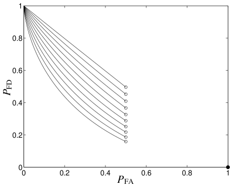
Figure 5: Sample false dismissal versus false alarm curves for the cross correlation statistic $\Lambda_{\text{CC}}$ in the large $N$ limit, as prescribed by Eq. (LABEL:specialized_analytic). For these curves the signal-to-noise ratio $\rho$ has equally spaced values from 0.01 to 1. Note that here $P_{\text{FD}}$ is undefined for $1/2\leq P_{\text{FA}}<1$.

The discontinuities at $P_{\text{FA}}=1/2$ are a result of the step functions in the definition (41) of $\hat{\alpha}^{2}$.

IV.1.2 Burst statistic

By combining the definition (9) of the burst statistic together with the decomposition (6), the noise and signal distributions (31) and (49), and the change of variables (57) it is straightforward to derive the exact false alarm versus false dismissal relation. The result is given by

$$(1-P_{\rm FA})^{1/N}={\rm erf}\left({\Lambda_{*}\over\sqrt{2}}\right)$$ (66)

and

$$P_{\rm FD}^{1/N}=\xi\,{\rm erf}\left[{\Lambda_{*}\over\sqrt{2+{2\rho\over\xi\sqrt{N}}}}\right]+(1-\xi)\,{\rm erf}\left({\Lambda_{*}\over\sqrt{2}}\right),$$ (67)

where $\Lambda_{*}$ is the value of the threshold.

IV.1.3 Maximum likelihood statistic

We start by discussing the different regimes present in the space of signal parameters $\xi$, $\rho$ and $N$, treating the false alarm probability $P_{\text{FA}}$ as fixed. There are several different constraints on the three parameters $\xi$, $\rho$, and $N$ that define the regime in parameter space where we expect our maximum likelihood statistic to work well. First, it is clear that the total number of events $\sim\xi N$ in the data set must be large compared to one:

$$\xi\gg\frac{1}{N}.$$ (68)

Second, if the signal-to-noise ratio $\alpha^{2}/(\sigma_{1}\sigma_{2})$ of individual burst events is large compared to one, then one can detect the individual events using the burst statistic (9) and the method of this paper is not needed. From Eq. (48) we can write the constraint $\alpha^{2}/(\sigma_{1}\sigma_{2})\lesssim 1$ as

$$\xi\gtrsim\frac{\rho}{\sqrt{N}}.$$ (69)

A more precise version of this requirement can be obtained by noting that the detection threshold for the signal-to-noise ratio $\alpha^{2}/(\sigma_{1}\sigma_{2})$ is $\sim\sqrt{2\ln N}$, since there are $N$ independent trials. This yields the constraint

$$\xi\gtrsim\frac{\rho}{\sqrt{2N\ln N}}.$$ (70)

The regime $\xi\sim\rho/\sqrt{2N\ln N}$ is where the burst statistic $\Lambda_{\text{B}}$ starts becoming as sensitive as the cross correlation statistic, as can be seen by combining Eqs. (LABEL:specialized_analytic), (66) and (67) above. This behavior can also be seen in Figs. 1 and 2 above.

A third constraint on the space of signal parameters is derived as follows. Consider the statistic

$$\eta=\frac{1}{N}\sum_{k=1}^{N}(h_{1}^{k})^{2}(h_{2}^{k})^{2}.$$ (71)

We can use this statistic to estimate the Gaussianity parameter $\xi$ in the following way. The mean value of $\eta$ when a signal is present is given by

$$\left<\eta\right>=3\xi\alpha^{4}+\xi\alpha^{2}(\sigma_{1}^{2}+\sigma_{2}^{2})+\sigma_{1}^{2}\sigma_{2}^{2},$$ (72)

and the variance when a signal is absent is

$$(\Delta\eta)^{2}=\sigma^{4}_{1}\sigma^{4}_{2}\frac{8}{N}.$$ (73)

It follows from Eqs. (72), (73), and the relation $\left<\hat{\alpha}^{2}\right>=\xi\alpha^{2}$ that the estimator ${\hat{\xi}}$ of $\xi$ defined by

$$\hat{\xi}=\frac{3\hat{\alpha}^{4}}{\eta-\hat{\alpha}^{2}(\hat{\sigma}_{1}^{2}+\hat{\sigma}_{2}^{2})-\hat{\sigma}_{1}^{2}\hat{\sigma}_{2}^{2}}$$ (74)

has a fractional accuracy of order

$$\frac{\Delta\xi}{\xi}\sim\frac{\xi\sqrt{N}}{\rho^{2}}.$$ (75)

Now in the regime $\Delta\xi/\xi\ll 1$, we expect our maximum likelihood detection statistic to work well, since one’s first guess for a nonlinear statistic (71) can be used to detect the non-Gaussianity of the signal to high accuracy. In the regime $\Delta\xi/\xi\gg 1$, it is not obvious how the maximum likelihood detection statistic will perform, since it could have a performance much better than that of the statistic $\eta$. However, our Monte Carlo simulations [Sec. IV.2 below] and analytic computations [Appendix C] indicate that the maximum likelihood statistic does indeed perform poorly in the regime $\Delta\xi/\xi\gg 1$. Thus, our third constraint is $\Delta\xi/\xi\lesssim 1$, which from Eq. (75) can be written as

$$\xi\lesssim\frac{\rho^{2}}{\sqrt{N}}.$$ (76)

Our Monte Carlo simulations show that for $\rho^{2}/\sqrt{N}\lesssim\xi\lesssim 1$, the maximum likelihood and cross-correlation statistics perform roughly equivalently, and that once $\xi$ becomes smaller than $\rho^{2}/\sqrt{N}$, the maximum likelihood statistic starts to perform significantly better than the cross-correlation statistic; see Figs. 1 and 2 above.

In Appendix C we derive analytically the approximate expression (168) for the false dismissal probability for the maximum likelihood statistic, which we expect to be accurate up to corrections of order $1/\rho^{4}$ or a few tens of percent. We also derive the expression (177) for the false alarm probability using a combination of analytical and numerical techniques. Combining these results gives the curves which are associated with the maximum likelihood statistic $\Lambda_{\text{ML}}^{\text{NG}}$ and labeled “analytic” in Figs. 1, 2, 9, and 10.

IV.2 Description of the Monte Carlo simulation algorithm

Next we describe our Monte Carlo simulations of the performances of the various statistics. We numerically estimate the false dismissal and false alarm probabilities $P_{\text{FD}}$ and $P_{\text{FA}}$ by conducting an ensemble of $N_{E}$ simulated experiments. For each experiment we simulate a detector output matrix, half of which have a signal present, and half of which do not. Since we know in advance whether or not a signal is present, we can easily estimate $P_{\text{FA}}$ and $P_{\text{FD}}$. More specifically, our algorithm for simulating false dismissal versus false alarm curves, for an arbitrary statistic $\Gamma$, is as follows:

1. Choose values for $\xi$, $\alpha$, $\sigma_{1}$, $\sigma_{2}$, and $N$.

2. Choose the total number of trials $N_{E}$.

3. For $r=1,2,\ldots,N_{E}/2$:

   1. Generate a data train $h(\sigma_{1},\sigma_{2},N)$ of noise only.

   2. Compute $\Gamma$ and store result as $\Gamma_{r0}$.

   3. Generate a data train $h(\xi,\alpha,\sigma_{1},\sigma_{2},N)$ which has a signal present.

   4. Compute $\Gamma$ and store result as $\Gamma_{r1}$.

4. Choose a discretization $\Gamma_{*j}$ of the set of thresholds, where $j=1,2,\ldots,M$.

5. Set $P_{\text{FA}}(\Gamma_{*j})=P_{\text{FD}}(\Gamma_{*j})=0$, for each $j$.

6. For $r=1,2,\ldots,N_{E}/2$:

   1. for each $j$, if $\Gamma_{r0}>\Gamma_{*j}$, increment $P_{\text{FA}}(\Gamma_{*j})$ by $2/N_{E}$.

   2. for each $j$, if $\Gamma_{r1}\leq\Gamma_{*j}$, increment $P_{\text{FD}}(\Gamma_{*j})$ by $2/N_{E}$.

7. Repeat steps 3-6 above several times to estimate the fluctuations in $P_{\text{FA}}(\Gamma_{*j})$ and $P_{\text{FD}}(\Gamma_{*j})$.

We use the above algorithm to simulate false dismissal versus false alarm curves for the three statistics $\Lambda_{\text{CC}}$, $\Lambda_{\rm B}$ and $\Lambda_{\text{ML}}^{\text{NG}}$. The analytical expressions (63) and (66) – (67) for the cross-correlation and burst statistics are used as a check of the numerical method.

IV.3 Simulation results

A family of simulated false dismissal versus false alarm curves for the cross correlation statistic $\Lambda_{\text{CC}}$ and the maximum likelihood statistic $\Lambda_{\text{ML}}^{\text{NG}}$ is shown in Fig. 6.

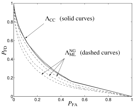
Figure 6: Plots of false dismissal probability ($P_{\text{FD}}$) versus false alarm probability ($P_{\text{FA}}$) for the standard cross-correlation statistic $\Lambda_{\text{CC}}$ and our maximum likelihood statistic $\Lambda_{\text{ML}}^{\text{NG}}$. Each of these curves is characterized by a total number of trials $N_{E}=2\times 10^{4}$, number of data points $N=5\times 10^{4}$, noise variances $\sigma_{1}=\sigma_{2}=1$, and by the signal-to-noise ratio $\rho=1$. The values of the Gaussianity parameter $\xi$ are 0.02, 0.012, and 0.01. The solid curves are the results for $\Lambda_{\rm ML}^{\rm G}$; these curves are bunched together because $\rho$ is fixed. The dashed curves are the results for $\Lambda_{\rm ML}^{\rm NG}$. For the dashed curves, the lowest curve is for $\xi=0.01$, while the highest curve is for $\xi=0.02$. We estimate error bars for each of these curves by separating the $2\times 10^{4}$ runs into 10 bins of $2\times 10^{3}$, and generating 10 separate plots; the resulting fluctuations are $\lesssim 10^{-3}$. The curves for the cross correlation statistic $\Lambda_{\rm ML}^{\rm G}$ agree with the analytic prediction (63) to within $\sim 10^{-3}$. This plot shows that $\Lambda_{\text{ML}}^{\text{NG}}$ can perform significantly better than $\Lambda_{\text{CC}}$.

We see that at fixed $\rho$, as the Gaussianity $\xi$ of the signal decreases, $\Lambda_{\text{ML}}^{\text{NG}}$ performs increasingly better than $\Lambda_{\text{CC}}$. The curves for $\Lambda_{\text{CC}}$ are almost indistinguishable from each other because $\rho$ is fixed, and the curves depend only on $\rho$ and not on $\xi$ for this detection statistic in the large $N$ limit [cf. Eq. (LABEL:specialized_analytic) above].

If we maintain the same value for $\rho$ as in Fig. 6, but take $\xi\gtrsim 0.03$, the curves for $\Lambda_{\text{CC}}$ and $\Lambda_{\text{ML}}^{\text{NG}}$ cannot be distinguished from each other. We find in general that for any values of $N$, $\sigma_{1}$, $\sigma_{2}$, and $\rho$, as $\xi\rightarrow 1$, the false dismissal versus false alarm curves for $\Lambda_{\text{CC}}$ and $\Lambda_{\text{ML}}^{\text{NG}}$ cannot be distinguished from each other. Thus, the two statistics are nearly equivalent for Gaussian signals, as expected. However, for $\xi\ll 1$, Fig. 6 demonstrates that $\Lambda_{\text{ML}}^{\text{NG}}$ performs noticeably better than $\Lambda_{\text{CC}}$.

We now discuss a comparison of the two statistics in terms of the minimum gravitational wave energy density necessary for detection, instead of in terms of the false dismissal versus false alarm curves. For a stochastic background with rms strain amplitude $h_{\text{rms}}$, we have $\Omega\propto h^{2}_{\text{rms}}$ Allen Review , where $\Omega$ is the gravitational wave energy density. For our model signal (49) we have $h_{\rm rms}^{2}\propto\xi\alpha^{2}$, and comparing this with the formula $\rho\propto\xi\alpha^{2}$ from Eq. (57) shows that we can interpret the signal to noise ratio $\rho$ as the energy density in the stochastic background, even for non-Gaussian signals.

We compute the minimum detectable energy density or signal-to-noise ratio $\rho_{\rm detectable}$ as follows. First, we choose thresholds $P_{\text{FA}*}$ and $P_{\text{FD}*}$ for the false alarm and false dismissal probabilities. We refer to the pair $(P_{\text{FA}*},P_{\text{FD}*})$ as the detection point. For any statistic $\Gamma$, the choice of detection point determines the detection threshold $\Gamma_{*}$, and inverting Eq. (60) gives the minimum detectable signal-to-noise ratio

$$\rho=\rho_{\text{detectable}}(P_{\text{FA}*},P_{\text{FD}*},\xi,N),$$ (77)

as illustrated in Fig. 7.

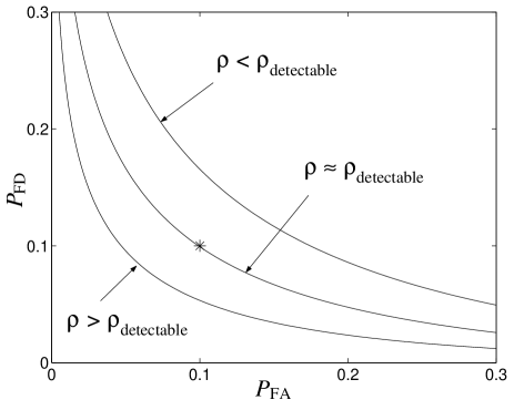
Figure 7: A family of false dismissal versus false alarm curves for fixed $\xi$. Here the detection point, at $P_{\text{FD}*}=P_{\text{FA}*}=0.1$, is marked with $*$.

For the cross-correlation statistic $\Lambda_{\text{CC}}$ the result is, from Eq. (63),

$$\rho_{\text{detectable}}^{\text{CC}} = \frac{2\sqrt{2}\gamma\left[1+\gamma\sqrt{2/N}\right]}{1+2\gamma^{2}\left(1-\frac{3}{\xi}\right)/N}\left[1+O\left({1\over\sqrt{N}}\right)\right]$$

$$= 2\sqrt{2}\gamma+O\left(\frac{1}{\sqrt{N}}\right)+O\left({\gamma\over\sqrt{N}}\right),$$

where $\gamma=\operatorname{erfc}^{-1}(2P_{\text{FA}*})$ and we have assumed that $P_{\text{FA}*}=P_{\text{FD}*}$. This relation is plotted in Fig. 8.

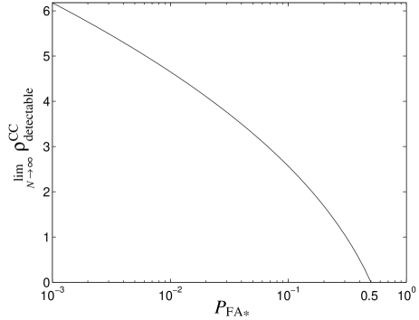
Figure 8: The minimum detectable signal-to-noise ratio $\rho_{\text{detectable}}^{\text{CC}}$ for the cross-correlation statistic $\Lambda_{\text{CC}}$ as a function of the false alarm probability threshold $P_{\text{FA}*}$. Note that we assume the false dismissal probability threshold $P_{\text{FD}*}=P_{\text{FA}*}$.

From the results of our simulations, we determine $\rho_{\text{detectable}}(P_{\text{FA}*},P_{\text{FD}*},\xi,N)$ by numerically solving the equation

$$P_{\text{FD}}(P_{\text{FA}*},\xi,\rho,N)-P_{\text{FD}*}=0$$ (80)

for $\rho$. Unfortunately, evaluating the function on the left hand side of Eq. (80) is computationally expensive. Each evaluation involves simulating the false dismissal versus false alarm curve which is itself a computationally intensive task. Moreover, it is only feasible for us to solve Eq. (80) for values of $N$ $\lesssim 10^{4}$ while a realistic detection scenario for ground based detectors would involve a year’s worth of data sampled at $\sim 100$ Hz for which $N\sim 10^{9}$. Therefore our conclusions about the applicability of the method to ground based detectors are based on our analytic results, as discussed in the Introduction.

Figure 9 shows the results obtained from numerically solving Eq. (80) for $\rho_{\rm detectable}$ for the parameter values $\xi=0.02$, $P_{\text{FA}*}=P_{\text{FD}*}=0.1$, and Fig. 10 shows the corresponding results for $\xi=4.3\times 10^{-3}$. For the cross-correlation statistic, the results are in good agreement with the analytic prediction (LABEL:analytic_detectable).

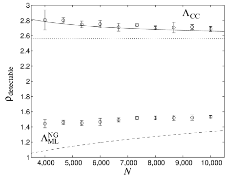
Figure 9: The minimum detectable signal strength $\rho_{\text{detectable}}$ as a function of the number of data points $N$, for the false alarm probability threshold $P_{\text{FA}*}=0.1$, false dismissal probability threshold $P_{\text{FD}*}=0.1$, and Gaussianity parameter $\xi=0.02$. The circles are the simulation results, and the error bars are estimated from ten different runs. The solid curve is the analytical prediction (LABEL:analytic_detectable) for $\Lambda_{\text{CC}}$, and the dotted line is the $N\to\infty$ limit (LABEL:specialized_detectable). The dashed line is the analytic prediction for $\Lambda_{\rm ML}^{\rm NG}$ given by Eqs. (168) and (177).

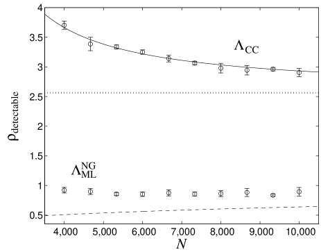
Figure 10: Same as Fig. 9 but with $\xi=4.3\times 10^{-3}$.

Figure 1 shows the minimum detectable energy density as a function of the Gaussianity parameter $\xi$ for $N=10^{4}$ (corresponding to space based detectors), for the cross-correlation and maximum likelihood statistics and also for the burst statistic (9). We again use the values $P_{\text{FA}*}=P_{\text{FD}*}=0.1$. The figure shows that the maximum likelihood statistic performs better than the other statistics by a factor which is roughly 3 for $\xi$ of order 1%. For smaller values of $\xi$, the maximum likelihood performs increasingly better than the cross-correlation statistic, but is eventually comparable to the burst statistic. Thus the maximum likelihood statistic gives an improvement in sensitivity to backgrounds composed of roughly $10$ to $10^{3}$ events per year.

Figure 2 is a similar plot, without the Monte Carlo simulation results, for $N=10^{9}$ (corresponding to ground based detectors). Here we use $P_{\text{FA}*}=P_{\text{FD}*}=0.01$. The results are similar to those in Fig. 1, except that here the gain in sensitivity occurs in the band $10^{-5}<\xi<10^{-3}$. This band corresponds to $10^{4}$-$10^{6}$ events per year.

IV.4 Parameter estimation

The computation of the maximum likelihood statistic also serves to measure the parameters of the signal. The statistic $\Lambda_{\text{ML}}^{\text{NG}}$, from Eq. (52), can be written as

$$\Lambda_{\text{ML}}^{\text{NG}}=\max_{0<\xi\leq 1}~{}\max_{\alpha^{2}>0}~{}\max_{\sigma^{2}_{1}\geq 0}~{}\max_{\sigma^{2}_{2}\geq 0}~{}\lambda(\xi,\alpha^{2},\sigma^{2}_{1},\sigma^{2}_{2}).$$ (81)

The point $(\hat{\xi},\hat{\alpha}^{2},\hat{\sigma}_{1}^{2},\hat{\sigma}^{2}_{2})$ where this maximum is achieved is the maximum likelihood estimator for $(\xi,\alpha^{2},\sigma_{1}^{2},\sigma^{2}_{2})$. In Fig. 11 we show contours of the function $\ln\lambda$ for a strong ($\rho=20$) signal.

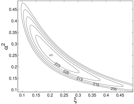
Figure 11: Representative contours of $\ln\lambda(\xi,\alpha^{2},\hat{\sigma}_{1}^{2},\hat{\sigma}_{2}^{2})$. Here $\rho=20$ and $N=1.6\times 10^{5}$. The simulated signal is characterized by $\xi=0.2$ and $\alpha^{2}=0.25$, marked with an $\times$. The noise is characterized by $\sigma_{1}^{2}=\sigma_{2}^{2}=1$. The maximum, marked with a $+$, is found at $\ln\lambda(0.207,0.251,0.993,0.993)=229$, while $\ln\lambda(0.2,0.25,1,1)=227$.

This figure shows that both $\xi$ and $\alpha^{2}$ can be measured with good accuracy.

Note that the main benefit of using $\Lambda_{\rm ML}^{\rm NG}$ is that it allows us to detect signals that are too weak to be seen using $\Lambda_{\text{CC}}$. Using $\Lambda_{\text{ML}}^{\text{NG}}$ also allows one to test if a detected signal is Gaussian, as obtained above, but this is not the main benefit of the method, as there are other, simpler, methods to test for non-Gaussianity.

V Conclusions

The use of our maximum likelihood statistic in searches for a non-Gaussian background gives a gain in sensitivity over the standard cross-correlation statistic. Figures 1 and 2 show that the gain factor can be significant for sufficiently non-Gaussian signals. However, computing the maximum likelihood statistic requires significantly more computational power than the cross-correlation statistic.

The analysis presented here must be generalized in several ways before being usable in gravitational wave detectors. These generalizations, listed in order of importance, are:

• Our signal model (49) assumes a Gaussian distribution of amplitudes of the burst events. This assumption simplified our analysis and resulted in a statistic with the useful property of being nearly equivalent to the cross-correlation statistic in the Gaussian signal limit. In practice however, the distribution of the events should instead be based on the candidate sources. For example, a popcorn-like stochastic background produced by a spatially uniform distribution of standard-candle sources out to some maximum redshift would have a signal distribution of the form (49) with the Gaussian term replaced by a term proportional to $s^{-4}\theta(s-s_{\min})$, where $\theta$ is the step function and $s_{\rm min}$ is a cutoff signal strength.

• One should allow the burst durations to be longer than the detector resolution time. For this situation one possibility would be to preprocess the data with a lowpass filter, and then apply the techniques developed here. Another possibility would be to try to combine the analysis of this paper with the excess power detection method of Ref. excess power .

• Real detector noise always contains non-Gaussian components, so one needs to generalize the analysis to allow for this. Such a generalization for a Gaussian stochastic background can be found in Refs. robust gaussian ; robust gaussian II .

• It would be useful to consider a more general signal model which consists of a superposition of a Gaussian background and a non-Gaussian background, since the true gravitational wave background might consist of such a superposition.

• The analysis needs to be generalized to allow for colored detector noise, and separated, misaligned detectors. This generalization should be fairly straightforward.

Appendix A General form of the likelihood ratio

In this appendix we give two derivations of the general formula (24) for the likelihood ratio. The first derivation is based on Eq. (22) while the second is based on Eq. (23). We also derive the formula (27) for the posterior probability density $p^{(1)}_{\mathcal{V}_{s},\mathcal{V}_{n}|\mathcal{T}}({\bf v}_{s},{\bf v}_{n}|1)$.

A.1 First derivation

We can derive Eq. (24) by using the total probability theorem to expand the distributions in the numerator and denominator of Eq. (22). Note that all distributions in this derivation are priors.

First expand $p_{\mathcal{H}}(h)$ just in terms of the random variable $\mathcal{T}$

$$p_{\mathcal{H}}(h)=P_{\mathcal{T}}(1)p_{\mathcal{H|T}}(h|1)+P_{\mathcal{T}}(0)p_{\mathcal{H|T}}(h|0).$$ (82)

Expanding $p_{\mathcal{H}}(h)$ in terms of all the degrees of freedom yields

$$p_{\mathcal{H}}(h)=\sum_{t=0}^{1}~{}\int_{\Theta_{s}}d^{Q_{s}}v_{s}~{}\int d^{ND}s~{}\int_{\Theta_{n}}d^{Q_{n}}v_{n}$$ (83)

$$~{}\times~{}p_{\mathcal{H|T,V}_{s},\mathcal{S,V}_{n}}(h|t,{\bf v}_{s},s,{\bf v}_{n})p_{\mathcal{T,V}_{s},\mathcal{S,V}_{n}}(t,{\bf v}_{s},s,{\bf v}_{n}),.$$

The ratio of the coefficients of $P_{\mathcal{T}}(1)$ and $P_{\mathcal{T}}(0)$ in Eq. (83) will give the general expression for the likelihood ratio by Eq. (22).

The conditional distribution for $\mathcal{H}$ in Eq. (83) can be translated into a conditional distribution for $\mathcal{N}$. From Eq. (10) it follows that

$$p_{\mathcal{H|S}}(h|s)=p_{\mathcal{N+S|S}}(h|s)=p_{\mathcal{N|S}}(h-s|s),$$ (84)

and since $\mathcal{S}$ and $\mathcal{N}$ are statistically independent we obtain

$$P_{\mathcal{H|S}}(h|s)=P_{\mathcal{N}}(h-s).$$ (85)

Generalizing this argument gives

$$p_{\mathcal{H|T,V}_{s},\mathcal{S,V}_{n}}(h|t,{\bf v}_{s},s,{\bf v}_{n})=p_{\mathcal{N|V}_{n}}(h-s|{\bf v}_{n}),$$ (86)

since a priori $\mathcal{T}$, $\mathcal{V}_{s}$, and $\mathcal{S}$ are statistically independent of $\mathcal{N}$ and $\mathcal{V}_{n}$. For the same reason we can write the joint distribution that appears in Eq. (83) as

$$p_{\mathcal{T,V}_{s},\mathcal{S,V}_{n}}(t,{\bf v}_{s},s,{\bf v}_{n})=p_{\mathcal{T,V}_{s},\mathcal{S}}(t,{\bf v}_{s},s)p_{\mathcal{V}_{n}}({\bf v}_{n}).$$ (87)

Substituting Eqs. (86) and (87) into Eq. (83) yields

$$p_{\mathcal{H}}(h) = \sum_{t=0}^{1}~{}\int_{\Theta_{s}}d^{Q_{s}}v_{s}~{}\int d^{ND}s~{}\int_{\Theta_{n}}d^{Q_{n}}v_{n}$$

$$\times p_{\mathcal{N|V}_{n}}(h-s|{\bf v}_{n})p_{\mathcal{T,V}_{s},\mathcal{S}}(t,{\bf v}_{s},s)p_{\mathcal{V}_{n}}({\bf v}_{n}).$$

We can also rewrite the distribution $p_{\mathcal{T,V}_{s},\mathcal{S}}(t,{\bf v}_{s},s)$ as

$$p_{\mathcal{T,V}_{s},\mathcal{S}}(t,{\bf v}_{s},s)=p_{\mathcal{S|V}_{s},\mathcal{T}}(s|{\bf v}_{s},t)p_{\mathcal{V}_{s}|T}({\bf v}_{s},t)P_{\mathcal{T}}(t),$$ (89)

by Eq. (14). Substituting Eq. (89) into Eq. (A.1) and explicitly evaluating the sum over $t$ yields

$$p_{\mathcal{H}}(h) = P_{\mathcal{T}}(1)\int_{\Theta_{s1}}d^{Q_{s}}v_{s}~{}\int d^{ND}s~{}\int_{\Theta_{n}}d^{Q_{n}}v_{n}~{}p_{\mathcal{N|V}_{n}}(h-s|{\bf v}_{n})p_{\mathcal{V}_{n}}({\bf v}_{n})p_{\mathcal{S|V}_{s},\mathcal{T}}(s|{\bf v}_{s},1)p_{\mathcal{V}_{s}|\mathcal{T}}({\bf v_{s}}|1)$$ (90)

$$+ P_{\mathcal{T}}(0)\int_{\Theta_{n}}d^{Q_{n}}v_{n}~{}p_{\mathcal{N|V}_{s}}(h|{\bf v}_{n}).$$

Here we have used the following relations:

$$p_{\mathcal{S|V}_{s},\mathcal{T}}(s|{\bf v}_{s}\in\Theta_{s1},0) = \delta^{ND}(s)$$ (91)

$$p_{\mathcal{V}_{s}|\mathcal{T}}({\bf v_{s}}\in\Theta_{s0}|1) = 0$$ (92)

$$p_{\mathcal{V}_{s}|\mathcal{T}}({\bf v_{s}}\in\Theta_{s1}|0) = 0$$ (93)

$$\int_{\Theta_{s0}}d^{Q_{s}}v_{s}~{}p_{\mathcal{V}_{s}|\mathcal{T}}({\bf v}_{s}|0) = 1.$$ (94)

By comparing Eqs. (82) and (90) we can read off the distributions $p_{\mathcal{H|T}}(h|t)$ and construct Eq. (24) from Eq. (22). Note that the expression (22) is independent of the space $\Theta_{s0}$ of signal parameters corresponding to “no signal present”.

A.2 Second derivation

Here we derive Eq. (24), and also Eq. (27), from Eq. (23). Consider the distribution

$$p_{\mathcal{T,V}_{s},\mathcal{V}_{n}|\mathcal{H}}(1,{\bf v}_{s},{\bf v}_{n}|h)=\frac{p_{\mathcal{T,V}_{s},\mathcal{V}_{n},\mathcal{H}}(1,{\bf v}_{s},{\bf v}_{n},h)}{p_{\mathcal{H}}(h)}.$$ (95)

We will justify Eq. (24) by the defining relation Eq. (23), which explicitly refers to priors and posteriors. Therefore we now append the appropriate superscripts as bookkeeping devices. Eq. (95) then reads

$$p^{(1)}_{\mathcal{T,V}_{s},\mathcal{V}_{n}}(1,{\bf v}_{s},{\bf v}_{n})=\frac{p^{(0)}_{\mathcal{T,V}_{s},\mathcal{V}_{n},\mathcal{H}}(1,{\bf v}_{s},{\bf v}_{n},h)}{p^{(0)}_{\mathcal{H}}(h)}.$$ (96)

Using the expansion of $p_{\mathcal{H}}(h)$ given by Eq. (90), and what we will justify is the likelihood ratio $\Lambda$ given by Eq. (24), we have

$$p^{(1)}_{\mathcal{T,V}_{s},\mathcal{V}_{n}}(1,{\bf v}_{s},{\bf v}_{n})=\frac{\left[\frac{p^{(0)}_{\mathcal{T,V}_{s},\mathcal{V}_{n},\mathcal{H}}(1,{\bf v}_{s},{\bf v}_{n},h)}{\int_{\Theta_{n}}d^{Q_{n}}v_{n}^{\prime}~{}p^{(0)}_{\mathcal{H|V}_{n}}(h|{\bf v}_{n})p^{(0)}_{\mathcal{V}_{n}}({\bf v}_{n})}\right]}{\Lambda P^{(0)}+1-P^{(0)}}.$$ (97)

Expanding the uppermost numerator in Eq. (97) over $\mathcal{S}$ by the total probability theorem gives

$$p^{(0)}_{\mathcal{T,V}_{s},\mathcal{V}_{n},\mathcal{H}}(1,{\bf v}_{s},{\bf v}_{n},h) = \int d^{ND}s$$

$$\times p^{(0)}_{\mathcal{T,V}_{s},\mathcal{V}_{n},\mathcal{H,S}}(1,{\bf v}_{s},{\bf v_{n}},h,s),$$

and rewriting this gives

$$p^{(0)}_{\mathcal{T,V}_{s},\mathcal{V}_{n},\mathcal{H,S}}(1,{\bf v}_{s},{\bf v_{n}},h,s)=p^{(0)}_{\mathcal{N|V}_{s}}(h-s|{\bf v}_{s})$$

$$\times p^{(0)}_{\mathcal{V}_{n}}({\bf v}_{n})p^{(0)}_{\mathcal{S|V}_{s},\mathcal{T}}(s|{\bf v}_{s},1)p^{(0)}_{\mathcal{V}_{s}|\mathcal{T}}({\bf v}_{s},1)P^{(0)}.$$ (99)

After putting Eq. (A.2) into Eq. (A.2), substitute the result into Eq. (97). Using $\Lambda({\bf v}_{s},{\bf v}_{n})$ given by Eq. (26) then yields

$$P^{(1)}p^{(1)}_{\mathcal{V}_{s},\mathcal{V}_{n}|\mathcal{T}}({\bf v}_{s},{\bf v}_{n}|1)=\frac{\Lambda({\bf v}_{s},{\bf v}_{n})P^{(0)}}{\Lambda P^{(0)}+1-P^{(0)}}.$$ (100)

On the left hand side of Eq. (100) we have used

$$p^{(1)}_{\mathcal{T,V}_{s},\mathcal{V}_{n}}(1,{\bf v}_{s},{\bf v}_{n})=P^{(1)}p^{(1)}_{\mathcal{V}_{s},\mathcal{V}_{n}|\mathcal{T}}({\bf v}_{s},{\bf v}_{n}|1).$$ (101)

Integrate Eq. (100) over $\Theta_{n}$ and $\Theta_{s1}$ using Eq. (25) and the normalization requirement

$$\int_{\Theta_{s1}}d^{Q_{s}}v_{s}\int_{\Theta_{n}}d^{Q_{n}}v_{n}~{}p^{(1)}_{\mathcal{V}_{s},\mathcal{V}_{n}|\mathcal{T}}({\bf v}_{s},{\bf v}_{n}|1)=1$$ (102)

to get

$$P^{(1)}=\frac{\Lambda P^{(0)}}{\Lambda P^{(0)}+1-P^{(0)}}.$$ (103)

Use Eq. (103) and Eq. (100) to form the ratio on the left hand side of Eq. (27) . This justifies Eq. (27).

Integrate Eq. (27) over $\Theta_{n}$ and $\Theta_{s1}$ using Eq. (25) and Eq.( 102) to see that the defining relation Eq. (23) is satisfied and thus Eq. (24) is justified.

Appendix B Analytical expressions for false dismissal versus false alarm curves for cross-correlation statistic

This appendix derives the analytical form (63) of the false dismissal versus false alarm curves for the cross-correlation statistic $\Lambda_{\text{CC}}$ in the large $N$ limit, for both Gaussian and non-Gaussian signals. A derivation for Gaussian signals can be found in Sec. IV of Ref. Allen Romano .

As noted in Sec. III.2, the statistics $\Lambda_{\text{CC}}$ and $\hat{\alpha}^{2}$ are equivalent in the large $N$ limit. Thus, in this limit, the false dismissal versus false alarm curves can be found by evaluating Eqs. (61) and (IV.1.1) with $\Gamma$ replaced by $\hat{\alpha}^{2}$. The relation (41) between the statistics ${\bar{\alpha}}^{2}$ and ${\hat{\alpha}}^{2}$ implies the following relation between their probability distributions $p_{\hat{\alpha}^{2}|\mathcal{T}}(x|t)$ and $p_{\bar{\alpha}^{2}|\mathcal{T}}(x|t)$:

$$p_{\hat{\alpha}^{2}|\mathcal{T}}(x|t)=\theta(x)p_{\bar{\alpha}^{2}|\mathcal{T}}(x|t)+\delta(x)\,\int_{-\infty}^{0}dy\,p_{\bar{\alpha}^{2}|\mathcal{T}}(y|t).$$ (104)

Inserting this formula into Eqs. (61) and (IV.1.1) gives

$$P_{\text{FA}}(\hat{\alpha}^{2}_{*}) = \left\{\begin{array}[]{ll}\displaystyle\int_{\hat{\alpha}^{2}_{*}}^{\infty}dx~{}p_{\bar{\alpha}^{2}|\mathcal{T}}(x|0)&\text{ if }\hat{\alpha}^{2}_{*}>0\\ \displaystyle 1&\text{ if }\hat{\alpha}^{2}_{*}\leq 0\\ \end{array}\right.,$$ (107)

$$P_{\text{FD}}(\hat{\alpha}^{2}_{*}) = \left\{\begin{array}[]{ll}\displaystyle 1-\int_{\hat{\alpha}^{2}_{*}}^{\infty}dx~{}p_{\bar{\alpha}^{2}|\mathcal{T}}(x|1)&\text{ if }\hat{\alpha}^{2}_{*}>0\\ \displaystyle 0&\text{ if }\hat{\alpha}^{2}_{*}\leq 0\\ \end{array}\right..$$ (110)

In the large $N$ limit, the distribution $p_{\bar{\alpha}^{2}_{s}|\mathcal{T}}(x|t)$ must be Gaussian by the central limit theorem, and therefore this distribution is characterized entirely by its mean $\left<\bar{\alpha}^{2}_{t}\right>$ and variance $[\Delta(\bar{\alpha}^{2}_{t})]^{2}$. From Eqs. (10), (33), (40), (41) and (49), these are given by

$$\left<\bar{\alpha}^{2}_{0}\right> = 0$$ (112)

$$\Delta(\bar{\alpha}^{2}_{0}) = \frac{\sigma_{1}\sigma_{2}}{\sqrt{N}}$$ (113)

$$\left<\bar{\alpha}^{2}_{1}\right> = \xi\alpha^{2}$$ (114)

$$\Delta(\bar{\alpha}^{2}_{1}) = \sqrt{\frac{\xi\alpha^{4}(3-\xi)+\xi\alpha^{2}(\sigma_{1}^{2}+\sigma_{2}^{2})+\sigma_{1}^{2}\sigma_{2}^{2}}{N}}.$$

Substituting Gaussian distributions, with means and variances determined by Eqs. (112)-(LABEL:var1), into Eqs. (107) and (LABEL:Pfd) yields

$$P_{\text{FA}}(\hat{\alpha}^{2}_{*},\sigma_{1},\sigma_{2},N) = \left\{\begin{array}[]{ll}\displaystyle\frac{1}{2}\operatorname{erfc}\left(\frac{\hat{\alpha}^{2}_{*}}{\sigma_{1}\sigma_{2}}\sqrt{\frac{N}{2}}\right)&\text{ if }\hat{\alpha}^{2}_{*}>0\\ \displaystyle 1&\text{ if }\hat{\alpha}^{2}_{*}\leq 0\\ \end{array},\right.$$ (118)

$$P_{\text{FD}}(\hat{\alpha}^{2}_{*},\xi,\alpha,\sigma_{1},\sigma_{2},N) = \left\{\begin{array}[]{ll}\displaystyle 1-\frac{1}{2}\operatorname{erfc}\left[\left(\hat{\alpha}^{2}_{*}-\xi\alpha^{2}\right)\sqrt{\frac{N}{2\left[\xi\alpha^{4}(3-\xi)+\xi\alpha^{2}(\sigma_{1}^{2}+\sigma_{2}^{2})+\sigma_{1}^{2}\sigma_{2}^{2}\right]}}\right]&\text{ if }\hat{\alpha}^{2}_{*}>0\\ \displaystyle 0&\text{ if }\hat{\alpha}^{2}_{*}\leq 0\\ \end{array}\right..$$ (121)

If we now eliminate $\hat{\alpha}^{2}_{*}$ between Eqs. (118) and (LABEL:analytic2), change variables from $\alpha$ to $\rho$ using Eq. (57), and set $\sigma_{1}=\sigma_{2}$, we obtain Eq. (63).

Appendix C Asymptotic behavior of maximum likelihood statistic

In this appendix we derive the large-$N$ behavior of the maximum likelihood statistic $\Lambda^{\rm NG}_{\rm ML}$. From Eq. (52), we can write the statistic in the form

$$\Lambda_{\rm ML}^{\rm NG}(h)=\exp\left[N{\cal L}(h)\right]$$ (123)

with

$${\cal L}(h)=\max_{\sigma_{1},\sigma_{2},\xi,\alpha}\,g(\sigma_{1},\sigma_{2},\xi,\alpha,h)$$ (124)

where

$$g=\frac{1}{N}\sum_{k=1}^{N}\,g_{k}(\sigma_{1},\sigma_{2},\xi,\alpha),$$ (125)

and the function $g_{k}=g_{k}(\sigma_{1},\sigma_{2},\xi,\alpha)$ is given by

$$e^{g_{k}}=\xi A_{k}(\alpha)+(1-\xi)A_{k}(0)$$ (126)

with

$$A_{k}(\alpha) = {\exp\left[\frac{\left(\frac{h_{1}^{k}}{\sigma^{2}_{1}}+\frac{h_{2}^{k}}{\sigma^{2}_{2}}\right)^{2}}{2\left(\frac{1}{\sigma^{2}_{1}}+\frac{1}{\sigma^{2}_{2}}+\frac{1}{\alpha^{2}}\right)}-\frac{\left(h_{1}^{k}\right)^{2}}{2\sigma^{2}_{1}}-\frac{\left(h_{2}^{k}\right)^{2}}{2\sigma^{2}_{2}}+1\right]}$$ (127)

$$\times{{\bar{\sigma}}_{1}{\bar{\sigma}}_{2}\over\sqrt{\sigma^{2}_{1}\sigma^{2}_{2}+\sigma^{2}_{1}\alpha^{2}+\sigma^{2}_{2}\alpha^{2}}}.$$

We denote by ${\tilde{\sigma}}_{1}$, ${\tilde{\sigma}}_{2}$, ${\tilde{\xi}}$ and ${\tilde{\alpha}}$ the “true” parameters governing the distribution of the quantities $h_{1}^{k}$ and $h_{2}^{k}$ according to Eqs. (10), (31), (33), and (49), with untilded quantities replaced by the corresponding tilded quantities. [These “true parameters” were denoted by $\sigma_{1}$, $\sigma_{2}$, $\xi$ and $\alpha$ in the body of the paper.] We define ${\tilde{\rho}}$ to be the signal-to-noise ratio (57) with untilded quantities replaced by tilded quantities:

$${\tilde{\rho}}\equiv\frac{{\tilde{\xi}}{\tilde{\alpha}}^{2}\sqrt{N}}{{\tilde{\sigma}}_{1}{\tilde{\sigma}}_{2}}.$$ (128)

For simplicity, in this appendix we restrict attention to the case ${\tilde{\sigma}}_{1}={\tilde{\sigma}}_{2}$. Then, without loss of generality, we can take ${\tilde{\sigma}}_{1}={\tilde{\sigma}}_{2}=1$ by rescaling our units of strain amplitude.

We discuss separately the computation of the false alarm and false dismissal probabilities, as different techniques are required to compute each.

C.1 False dismissal probability

The false dismissal probability for the statistic (124) will be some function

$$P_{\rm FD}=P_{\rm FD}({\cal L}_{*},N,{\tilde{\xi}},{\tilde{\rho}})$$ (129)

of the threshold ${\cal L}_{*}$ on ${\cal L}$, the number of data points $N$, the Gaussianity parameter ${\tilde{\xi}}$ and signal-to-noise ratio ${\tilde{\rho}}$ of the signal. For applications to ground based detectors, we will have ${\tilde{\rho}}\sim$ (a few), in order that the signal be detectable, $N\sim 10^{9}$, and $10^{-3}\lesssim{\tilde{\xi}}\leq 1$. Therefore it would be useful to find approximate analytic expressions for the false alarm probability in the limit of large $N$. There are actually several different, large $N$ regimes in the three dimensional parameter space $(N,{\tilde{\xi}},{\tilde{\rho}})$ that one might explore:

• The limit $N\to\infty$ with ${\tilde{\alpha}}$ and ${\tilde{\xi}}$ held fixed. This corresponds to fixing the stochastic background signal and going to a limit of long observation times. In this limit we have ${\tilde{\rho}}\propto\sqrt{N}$ which diverges. This is not a very realistic limit to explore.

• The limit $N\to\infty$ with ${\tilde{\rho}}$ and ${\tilde{\xi}}$ held fixed. In this limit, the signal-to-noise ratio is held fixed, and correspondingly the amplitude ${\tilde{\alpha}}$ of the stochastic background signal goes to zero, from Eq. (128). This would be the most natural limit to explore. However, in this limit the statistical error $\Delta{\tilde{\xi}}$ in our measurement of the Gaussianity parameter would diverge, from Eq. (75), and therefore in this limit we do not expect to be able to compute analytically the value of the parameter $\xi$ which achieves the maximum in Eq. (124). The analytic approximation methods which we discuss below do not work in this regime. [In addition our Monte Carlo simulations show that the maximum likelihood statistic itself does not perform any better than the cross-correlation statistic in this regime, as discussed in the Introduction.]

• The limit we actually explore is the limit $N\to\infty$ with ${\tilde{\xi}}$ fixed and ${\tilde{\rho}}$ scaling $\propto N^{1/4}$, corresponding to ${\tilde{\alpha}}\propto N^{-1/8}$. The reason for our choosing to explore this particular limit is simply that it is amenable to analytic computations. Fractional corrections to our analytic results should scale like $1/N$ or as $1/{\tilde{\rho}}^{4}$. Since ${\tilde{\rho}}\sim$ (a few) at the threshold for detection, the approximation should be good to $10\%-20\%$ or so.

We now turn to a discussion of the computational technique. We write

$${\tilde{\alpha}}={\tilde{\alpha}}_{0}N^{-1/8},$$ (130)

where ${\tilde{\alpha}}_{0}$ is independent of $N$. Correspondingly, from Eq. (49) we can write

$$s^{k}=N^{-1/8}{\hat{s}}^{k},$$ (131)

where the distribution of ${\hat{s}}^{k}$ is given by Eq. (49) with $\xi$ replaced by ${\tilde{\xi}}$ and $\alpha$ replaced by ${\tilde{\alpha}}_{0}$. In particular, the distribution of ${\hat{s}}^{k}$ is independent of $N$. In computing the maximum over $(\xi,\alpha,\sigma_{1},\sigma_{2})$ in Eq. (124), it is useful change variables from $\alpha$ to $\kappa$ defined by

$$\kappa=\rho N^{-1/4}={\xi\alpha^{2}N^{1/4}\over\sigma_{1}\sigma_{2}},$$ (132)

which we expect to be independent of $N$ to leading order in the large $N$ limit. The value of the variable $\kappa$ that characterizes the signal is

$${\tilde{\kappa}}={\tilde{\rho}}N^{-1/4}={{\tilde{\xi}}{\tilde{\alpha}}_{0}^{2}\over{\tilde{\sigma}}_{1}{\tilde{\sigma}}_{2}};$$ (133)

cf. Eqs. (130) and (132).

We now consider fixed realizations of the infinite sequences of random variables $n_{1}^{k}$, $n_{2}^{k}$ and ${\hat{s}}^{k}$, and $1\leq k<\infty$, and examine the limiting behavior of ${\cal L}(h)$ as $N\to\infty$. We compute this limiting behavior by substituting into the right hand side of Eq. (123) the relations

$$h_{1}^{k}=n_{1}^{k}+N^{-1/8}{\hat{s}}^{k}\ \ \ \ \ h_{2}^{k}=n_{2}^{k}+N^{-1/8}{\hat{s}}^{k},$$ (134)

writing $\alpha$ in terms of $\kappa$ using Eq. (132), and expanding in powers of $N^{-1/8}$. The result is an expression which can be written in terms of the sums $Q_{abc}$ defined by

$$Q_{abc}=\frac{1}{N}\sum_{k=1}^{N}\left(\hat{s}^{k}\right)^{a}\left(n_{1}^{k}\right)^{b}\left(n_{2}^{k}\right)^{c},$$ (135)

where $a$, $b$, and $c$ are non-negative integers. From the central limit theorem we can write

$$Q_{abc}=\mu_{abc}+\frac{1}{\sqrt{N}}\Delta_{abc},$$ (136)

where $\mu_{abc}=\left<Q_{abc}\right>$ are computable functions of ${\tilde{\xi}}$ and ${\tilde{\alpha}}$, and where the random variables $(\Delta_{100},\Delta_{010},\ldots)$ converge in distribution as $N\rightarrow\infty$ to a multivariate Gaussian of zero mean whose variance-covariance matrix is independent of $N$. Thus, in particular the joint distribution of all $\Delta_{abc}$’s is $N$-independent in limit that $N\rightarrow\infty$.

We define the vector

$${\bf v}=(v^{1},v^{2},v^{3},v^{4})=(\xi,\kappa,\sigma_{1}^{2},\sigma_{2}^{2}),$$ (137)

We denote the value of ${\bf v}$ that achieves the maximum in Eq. (124) by $\hat{{\bf v}}$:

$$g(\hat{{\bf v}})=\max_{{\bf v}}~{}g({\bf v}),$$ (138)

where $\hat{{\bf v}}=(\hat{\xi},\hat{\kappa},\widehat{\sigma_{1}^{2}},\widehat{\sigma_{2}^{2}})$. These estimators satisfy a system of four equations

$$\left.\frac{\partial g}{\partial v^{l}}\right|_{{\bf v}=\hat{{\bf v}}}=0.$$ (139)

We solve Eq. (139) perturbatively. First assume that the estimators can be expanded in the form

$$\widehat{v^{l}}=\sum_{j=0}^{\infty}\widehat{v^{l}}^{[j]}\epsilon^{j},$$ (140)

where for ease of notation we have defined $\epsilon=N^{-1/8}$. We define the expansion coefficients $v^{l[j]}$ analogously by an expansion of the form (140) but without the hats. Now using Eq. (136) the function $g$ can be expanded as a power series in $\epsilon$ whose coefficients are functions of $v^{l[k]}$, $\mu_{abc}$, and $\Delta_{abc}$:

$$g({\bf v})=\sum_{j=0}^{\infty}g^{[j]}\left[v^{l[k]},\mu_{abc},\Delta_{abc}\right]\epsilon^{j}.$$ (141)

Substituting the expansions (140) and (141) into the condition (139) for a local extremum gives an infinite set of equations which must collectively be satisfied by the coefficients $\widehat{v^{l}}^{[j]}$

$$\left.\frac{\partial g^{[j]}}{\partial v^{l[k]}}\right|_{v^{m[n]}=\widehat{v^{m}}^{[n]}}=0.$$ (142)

We solve these equations order by order to determine the coefficients $\widehat{{v^{l}}}^{[j]}$, and thereby justify a posteriori the ansatz (140).

We find that in order to compute the leading order expression for ${\cal L}$, we must obtain the expansion for ${\hat{\xi}}$ to zeroth order in $\epsilon$, the expansion for ${\hat{\kappa}}$ to fourth order in $\epsilon$, and the expansions of ${\hat{\sigma_{1}^{2}}}$ and ${\hat{\sigma_{2}^{2}}}$ to sixth order in $\epsilon$. The leading order results are

$${\hat{\kappa}} = {\tilde{\kappa}}+\epsilon^{2}X+O(\epsilon^{3}),$$ (143)

$${1\over{\hat{\xi}}} = {1\over{\tilde{\xi}}}+{Y\over\sqrt{6}{\tilde{\kappa}}^{2}}+O(\epsilon),$$ (144)

$$\widehat{\sigma_{1}^{2}} = 1+O(\epsilon^{2}),$$ (145)

$$\widehat{\sigma_{2}^{2}} = 1+O(\epsilon^{2}),$$ (146)

where

$$X=\Delta_{011}$$ (147)

and

$$Y = {1\over 8\sqrt{6}}\bigg{[}4(\Delta_{031}+\Delta_{013})-12(\Delta_{002}+\Delta_{020})$$ (148)

$$-24\Delta_{011}+\Delta_{040}+\Delta_{004}+6\Delta_{022}\bigg{]}.$$

Using Eqs. (31), (49), (135) and (136) one can show that the random variables $X$ and $Y$ are independent Gaussian random variables of zero mean and unit variance.

In deriving Eqs. (143) – (146) we assumed that the value of ${\bf v}$ which achieves the maximum in Eq. (124) corresponds a local maximum. However, if the right hand side of Eq. (143) is negative, the maximum will instead be achieved on the boundary of the parameter space at ${\hat{\kappa}}=0$, since the variable $\kappa$ must be non-negative. Similarly, if the right hand side of Eq. (144) is less than 1, the maximum will be achieved at ${\hat{\xi}}=1$, since $1/\xi$ must lie in the interval $[1,\infty)$.

Substituting the results (143) – (146) [together with the higher order corrections to those results which we have not shown] into the expansion for the statistic ${\cal L}$, and taking into account the various special cases discussed in the last paragraph, gives

$${\cal L} = \bigg{[}{1\over 2}\left(Y+\sqrt{6}q{\tilde{\kappa}}^{2}\right)^{2}\epsilon^{8}\,\theta\left(Y+\sqrt{6}q{\tilde{\kappa}}^{2}\right)$$ (149)

$$+{1\over 2}({\tilde{\kappa}}+\epsilon^{2}X)^{2}\epsilon^{4}-{\tilde{\kappa}}^{3}\epsilon^{6}+{7\over 4}{\tilde{\kappa}}^{4}\epsilon^{8}$$

$$+{\tilde{\kappa}}U\epsilon^{7}+{\tilde{\kappa}}V\epsilon^{8}\bigg{]}\theta({\tilde{\kappa}}+\epsilon^{2}X)+O(\epsilon^{9}).$$

Here $\theta(x)$ is the step function and

$$q = {1\over{\tilde{\xi}}}-1,$$ (150)

$$U = \Delta_{101}+\Delta_{110},$$ (151)

$$V = \Delta_{200}-{1\over 2}{\tilde{\kappa}}(\Delta_{002}+\Delta_{020})-2{\tilde{\kappa}}\Delta_{011}.$$ (152)

We note that the corresponding expression for the statistic $(\ln\Lambda_{\rm ML}^{\rm G})/N$ [which is equivalent to the cross-correlation statistic by Eq. (43)] is given by Eq. (149) with the first term in the square brackets dropped.

Next we drop all the terms in the square bracket in Eq. (149) other than the first two terms. The reason is that these terms will give corrections that are smaller than the terms retained (both in expected value and in fluctuations) by a factor of

$${\tilde{\kappa}}\epsilon^{2}={{\tilde{\rho}}\over\sqrt{N}},$$

which will be small compared to unity for all cases we are interested in. This gives for the false dismissal probability the expression

$$P_{\text{FD}} = P({\cal L}<{\cal L}_{*})$$

$$= \int_{\cal R}{dxdy\over 2\pi}\exp\left[-{(x-x_{0})^{2}\over 2}-{(y-y_{0})^{2}\over 2}\right],$$

where

$$x_{0} = {\tilde{\kappa}}/\epsilon^{2}$$ (154)

$$y_{0} = \sqrt{6}q{\tilde{\kappa}}^{2}$$ (155)

$$r_{0} = \sqrt{2N{\cal L}_{*}}.$$ (156)

Here the region ${\cal R}$ in the $x,y$ plane is the union of the two regions

$$x \geq 0$$

$$y \geq 0$$

$$x^{2}+y^{2} \leq r_{0}^{2}$$ (157)

and

$$y \leq 0$$

$$0\leq x \leq r_{0}.$$ (158)

The integral over the region (158) is

$$P_{\rm FD}^{(1)}={\cal P}(-y_{0})[{\cal P}(r_{0}-x_{0})-{\cal P}(-x_{0})],$$ (159)

where

$${\cal P}(x)\equiv 1-{1\over 2}\operatorname{erfc}(x/\sqrt{2})=\int_{-\infty}^{x}dt{1\over\sqrt{2\pi}}\exp[-t^{2}/2].$$ (160)

The integral over the region (157) can be written as

$$P_{\rm FD}^{(2)} = {1\over 2\pi}\int_{0}^{\pi/2}d\theta\,\int_{0}^{r_{0}}dr\,r$$

$$\times \exp\left[-{1\over 2}(r\cos\theta-x_{0})^{2}-{1\over 2}(r\sin\theta-y_{0})^{2}\right].$$

The integrand in (LABEL:eq:pFD1) peaks at $r\cos\theta=x_{0}$, $r\sin\theta=y_{0}$. In order for $P_{\rm FD}$ to be small, its necessary that this peak occurs outside the domain of integration, at $r>r_{0}$. So we must have

$$x_{0}^{2}+y_{0}^{2}\geq r_{0}^{2}.$$ (162)

The criterion $x_{0}\geq r_{0}$ is, in order of magnitude, just the usual criterion for detectability with the cross-correlation statistic. The criterion $y_{0}\gtrsim r_{0}$ reduces to, in order of magnitude,

$$\xi\lesssim{\rho^{2}\over\sqrt{N}}$$ (163)

which is what we claimed earlier to be the regime where the maximum likelihood statistic starts to work well, cf. Sec. IV.1.3 above.

Evaluating the integral (LABEL:eq:pFD1) using the Laplace approximation gives

$$P_{\rm FD}^{(2)} = {1\over r_{0}(\lambda-1)\sqrt{2\pi\lambda}}\exp\left[-{1\over 2}r_{0}^{2}(\lambda-1)^{2}\right]$$ (164)

$$\times\left[1+O\left({1\over r_{0}}\right)\right],$$

where we define the variables $\lambda$ and $\gamma$ by

$$(x_{0},y_{0})=r_{0}\lambda(\cos\gamma,\sin\gamma).$$ (165)

However, the result (164) is not very accurate for small $r_{0}$. Alternatively we can integrate over $r$ in Eq. (LABEL:eq:pFD1) to obtain

$$P_{\rm FD}^{(2)}=\int_{0}^{\pi/2}d\theta\left\{\frac{1}{2\pi}e^{\frac{{{r_{0}}}^{2}\,\left(1+{\lambda}^{2}\right)}{2}}\left[e^{\frac{{{r_{0}}}^{2}}{2}}-e^{{{r_{0}}}^{2}\,\lambda\,\cos(\gamma-\theta)}\right]\right.$$

$$+\left.\frac{r_{0}\lambda}{2\sqrt{2\pi}}e^{\frac{{{r_{0}}}^{2}\lambda^{2}}{4}\left[\cos(2\,\left\{\gamma-\theta\right\})-1\right]}\cos\left(\gamma-\theta\right)\left[\operatorname{erf}\left(\frac{{r_{0}}\,\lambda\cos\{\gamma-\theta\}}{{\sqrt{2}}}\right)+\operatorname{erf}\left(\frac{{r_{0}}\,\left\{1-\lambda\,\cos[\gamma-\theta]\right\}}{{\sqrt{2}}}\right)\right]\right\},$$ (166)

where

$$\operatorname{erf}(x)=\frac{2}{\sqrt{\pi}}\int_{0}^{x}dy~{}e^{-y^{2}}.$$ (167)

The integral (166) can be evaluated numerically. The false dismissal probability is then given by

$$P_{\rm FD}=P_{\rm FD}^{(1)}+P_{\rm FD}^{(2)},$$ (168)

with $P_{\rm FD}^{(1)}$ given by Eq. (159) and $P_{\rm FD}^{(2)}$ given by Eq. (166).

C.2 False alarm probability

The false alarm probability is some function

$$P_{\rm FA}=P_{\rm FA}({\cal L}_{*},N)$$ (169)

of the threshold ${\cal L}_{*}$ value of the detection statistic (124) and of the number of data points $N$. It does not depend on the signal parameters ${\tilde{\rho}}$ and ${\tilde{\xi}}$ because no signal is present. We would like to evaluate this quantity in the large $N$ limit.

We start by rewriting the statistic (124) in the form

$${\cal L}=\max_{\bf v}\left\{{1\over N}\sum_{k=1}^{N}\ln A_{k}(0)+{1\over N}\sum_{k=1}^{N}\ln\left[1+\xi{\cal D}_{k}(\alpha)\right]\right\},$$ (170)

where

$${\cal D}_{k}(\alpha)={A_{k}(\alpha)\over A_{k}(0)}-1.$$ (171)

Consider first the first term in Eq. (170). Using the definition (127) of $A_{k}(\alpha)$ and the definition (4) of ${\bar{\sigma}}_{1}$ and ${\bar{\sigma}}_{2}$ we can write this term as

$${1\over N}\sum_{k=1}^{N}\ln A_{k}(0)=-{\Delta\sigma_{1}^{2}\over{\bar{\sigma}}_{1}^{2}}-{\Delta\sigma_{2}^{2}\over{\bar{\sigma}}_{2}^{2}}+O(\Delta\sigma_{1}^{3},\Delta\sigma_{2}^{3}),$$ (172)

where $\Delta\sigma_{1}=\sigma_{1}-{\bar{\sigma}}_{1}$, $\Delta\sigma_{2}=\sigma_{2}-{\bar{\sigma}}_{2}$. Therefore the first term is maximized at $\sigma_{1}={\bar{\sigma}}_{1}$, $\sigma_{2}={\bar{\sigma}}_{2}$. Below we shall show that the second term in Eq. (170) is of order $O(\epsilon^{2})$, where in this subsection we define $\epsilon=1/\sqrt{N}$. Therefore the values of $\sigma_{1}$ and $\sigma_{2}$ that achieve the maximum are

$${\hat{\sigma}}_{1} = {\bar{\sigma}}_{1}\left[1+O(\epsilon^{2})\right]$$

$${\hat{\sigma}}_{2} = {\bar{\sigma}}_{2}\left[1+O(\epsilon^{2})\right].$$ (173)

Moreover, in analyzing the second term it suffices to take $\sigma_{1}={\bar{\sigma}}_{1}$, $\sigma_{2}={\bar{\sigma}}_{2}$ in order to obtain the statistic to the leading $O(\epsilon^{2})$ order. Lastly, since we have assumed that ${\tilde{\sigma}}_{1}={\tilde{\sigma}}_{2}=1$ and no signal is present, we have ${\bar{\sigma}}_{1,2}=1+O(\epsilon)$. Hence, in analyzing the second term, it is sufficient to take $\sigma_{1}=\sigma_{2}=1$.

The statistic (170) therefore reduces to

$${\cal L}=\max_{\alpha,\xi}{1\over N}\sum_{k=1}^{N}\,\ln\left[1+\xi{\cal D}_{k}(\alpha)\right]+O(\epsilon),$$ (174)

where from Eqs. (127) and (171)

$${\cal D}_{k}(\alpha)={1\over\sqrt{1+2\alpha}}\exp\left[{w_{k}^{2}\over 2+{1\over\alpha}}\right]-1.$$ (175)

Here $w_{k}=(n_{1}^{k}+n_{2}^{k})/\sqrt{2}$, $1\leq k\leq N$, are independent Gaussian random variables of zero mean and unit variance.

It is straightforward to numerically compute the distribution of the statistic (174), by generating the Gaussian variables $w_{k}$ and numerically maximizing over $\xi$ and $\alpha$. The result is shown in Fig. 12. We find that at large $N$, the distribution of $N{\cal L}$ becomes independent of $N$, and is approximately given by

$$P(N{\cal L}>\xi)=\alpha_{0}e^{-\beta_{0}\xi}$$ (176)

for $\xi>0$, where $\alpha_{0}\approx 0.42$ and $\beta_{0}\approx 1.08$. Therefore the false alarm probability is approximately given by

$$P_{\rm FA}=\alpha_{0}\exp\left[-\beta_{0}N{\cal L}_{*}\right].$$ (177)

Figure 12: The cumulative distribution function for the leading order expression (174) for the statistic when no signal is present, obtained numerically. The solid line is for $N=1000$, and the dashed line for $N=5000$.

Finally, we remark why it is plausible to expect the distribution of $N{\cal L}$ to be independent of $N$ in the large $N$ limit. The numerical maximizations over $\xi$ and $\alpha$ in Eq. (174) show that the maximum is nearly always achieved at $\alpha\ll 1$ or $\xi\ll 1$. In both these regimes, one can obtain some information about the $N$-dependence of the statistic.

Consider first the regime $\xi\ll 1$. In this regime we can expand the expression (174) as a power series in $\xi$ to obtain

$${\cal L}=\max_{\alpha,\xi}{1\over N}\sum_{k=1}^{N}\,\left[\xi{\cal D}_{k}(\alpha)-{1\over 2}\xi^{2}{\cal D}_{k}(\alpha)^{2}+O(\xi^{3})\right]+O(\epsilon).$$ (178)

The generalized central limit theorem (reviewed in Appendix D) implies that

$${1\over N}\sum_{k=1}^{N}\,{\cal D}_{k}(\alpha)=N^{1-\gamma_{1}\over\gamma_{1}}\left(\ln N\right)^{\delta_{1}}{\cal F}_{N}(\alpha),$$ (179)

where for each fixed $\alpha$, the distribution of the random variable ${\cal F}_{N}(\alpha)$ becomes independent of $N$ in the large $N$ limit. Here

$$\gamma_{1}=\left\{\begin{array}[]{ll}2&0<\alpha\leq 1/2\\ 1+{1\over 2\alpha}&1/2\leq\alpha\\ \end{array}\right.$$ (180)

and

$$\delta_{1}=\left\{\begin{array}[]{ll}0&0<\alpha\leq 1/2\\ {-\alpha\over 1+2\alpha}&1/2\leq\alpha.\\ \end{array}\right.$$ (181)

The limiting distribution is a Levy distribution with parameters $p=1$ and $\gamma=\gamma_{1}$. Similarly we have

$${1\over N}\sum_{k=1}^{N}\,{\cal D}_{k}(\alpha)^{2}=N^{1-\gamma_{2}\over\gamma_{2}}\left(\ln N\right)^{\delta_{2}}{\cal G}_{N}(\alpha),$$ (182)

where as $N\to\infty$ at each fixed $\alpha$ the distribution of the random variable ${\cal G}_{N}(\alpha)$ tends to a Levy distribution with parameters $p=1$ and $\gamma=\gamma_{2}$, with

$$\gamma_{2}=\left\{\begin{array}[]{ll}2&0<\alpha\leq 1/6\\ {1+2\alpha\over 4\alpha}&1/6\leq\alpha.\\ \end{array}\right.$$ (183)

and

$$\delta_{2}=\left\{\begin{array}[]{ll}0&0<\alpha\leq 1/6\\ {-2\alpha\over 1+2\alpha}&1/6\leq\alpha.\\ \end{array}\right.$$ (184)

We now substitute the results (179) and (182) into the expression (178) for the statistic, and maximize analytically over the quadratic dependence on $\xi$. For $\alpha\geq 1/2$, the value of $\xi$ which achieves the maximum goes to zero as $N\to\infty$, consistent with the assumption $\xi\ll 1$, and the result is

$$N{\cal L}={1\over 2}\max_{\alpha}{{\cal F}_{N}(\alpha)^{2}\over{\cal G}_{N}(\alpha)}+O(\epsilon).$$ (185)

In the regime $\alpha\ll 1$, if we expand the expression (174) to quadratic order in $\alpha$, the result is an expression which is a linear function of $1/\xi$ at fixed $\alpha\xi$. Hence, when one maximizes over values of $\xi$ in the range $0\leq\xi\leq 1$, the maximum is always achieved either at $\xi=0$ or $\xi=1$. One can show that the maximum to this order is always achieved at $\xi=1$, and the resulting expression is

$$N{\cal L}={1\over 4}{\cal G}^{2}+O(\epsilon),$$ (186)

where

$${\cal G}=\sqrt{N}\left[{1\over N}\sum_{k=1}^{N}w_{k}^{2}\ -1\right]$$ (187)

has a distribution that is independent of $N$ in the large $N$ limit.

Appendix D Generalized central limit theorem

In this appendix we review the generalized central limit theorem that can be found on p. 574 of Ref. Feller . First we define a particular distribution function called the Levy distribution. It depends on 3 real parameters, a positive constant $C$, a parameter $\gamma$ in the range $0<\gamma\leq 2$, and constant $p$ in the range $0\leq p\leq 1$ . We say a random variable $X$ has a Levy distribution with parameters $C$, $\gamma$ and $p$ if the characteristic function of $X$ is given by

$$\left<e^{i\zeta X}\right> = \exp\bigg{\{}|\zeta|^{\gamma}{C\Gamma(3-\gamma)\over\gamma(\gamma-1)}\bigg{[}\cos(\pi\gamma/2)$$ (188)

$$+i\,{\rm sgn}(\zeta)(p-q)\sin(\pi\gamma/2)\bigg{]}\bigg{\}},$$

where $q=1-p$. The corresponding probability distribution function is obtained by taking a Fourier transform and decays like $x^{-(1+\gamma)}$ at large $x$ for $\gamma<2$ ($\gamma=2$ is the Gaussian case).

Consider now a random variable $X$ with probability distribution function $f(x)$ whose variance is infinite. Let

$$F(x)=\int_{-\infty}^{x}dy\,f(y)$$ (189)

be the cumulative distribution function and define

$$\mu(x)=\int_{-x}^{x}dyy^{2}f(y).$$ (190)

Suppose that the distribution satisfies the following conditions: (i) As $x\to\infty$ we have $\mu(x)\sim x^{2-\gamma}L(x)$, where $0<\gamma\leq 2$, and $L(x)$ varies slowly in the sense that $L(tx)/L(t)\to 1$ as $t\to\infty$ for all $x>0$. (ii) We have

$${1-F(x)\over F(-x)+1-F(x)}\to p\ \ \ \ \ {F(-x)\over F(-x)+1-F(x)}\to q$$ (191)

as $x\to\infty$, where $0\leq p\leq 1$, $0\leq q\leq 1$ and $p+q=1$. (iii) For $1<\gamma\leq 2$, we assume that the expected value $\int dx\,xf(x)$ vanishes; this can be enforced by making a transformation of the form $X\to X+{\rm constant}$.

We define the sequence of random variables

$$S_{N}={1\over a_{N}}\sum_{i=1}^{N}\,X_{i},$$ (192)

where the $X_{i}$ are independent, identically distributed random variables with distribution function $f$, and the constants $a_{N}$ are chosen to satisfy

$${N\mu(a_{N})\over a_{N}^{2}}\to C$$ (193)

as $N\to\infty$, where $C$ is a positive constant. Then, the distribution functions of the random variables $S_{N}$ converge to a Levy distribution with parameters $C$, $\gamma$ and $p$ as $N\to\infty$.

References

- (1) A. Abramovici et al., Science 256, 325 (1992).
- (2) C. Bradaschia et al., Nuc. Instrum. Methods 289, 518 (1990).
- (3) R. Schilling, AIP Conf. Proc. 456, 217 (1998).
- (4) M. K. Fujimoto, Journal of the Communications Research Laboratory 46, 437 (1999).
- (5) B. Allen, in Relativistic Gravitation and Gravitational Radiation, Proceedings of the Les Houches School of Physics, Les Houches, 1995, edited by J. A. Marck and J. P. Lasota (CNRS, Observatorie de Paris, Meudon, 1997), p. 373.
- (6) D. Blair and L. Ju, Mon. Not. R. Astron. Soc. 283, 648 (1996).
- (7) V. Ferrari, S. Matarrese, and R. Schneider, Mon. Not. R. Astron. Soc. 303, 247 (1999).
- (8) R. Schneider et al., Mon. Not. R. Astron. Soc. 317, 385 (2000).
- (9) V. Ferrari, S. Matarrese, and R. Schneider, Mon. Not. R. Astron. Soc. 303, 258 (1999).
- (10) T. Regimbau and J. A. de Freitas Pacheco, astro-ph/0105260.
- (11) T. Damour, A. Vilenkin, Phys. Rev D 64, 064008 (2002) (also gr-qc/0104026).
- (12) M. Kamionkowski, A. Kosowsky, and M. S. Turner, Phys. Rev. D 49, 2837 (1994).
- (13) L.P. Grishchuk, Zh. Eksp. Teor. Fiz. 67, 825 (1974) [Sov. Phys. JETP 40, 409 (1975)]; E.W. Kolb and M.S. Turner, The Early Universe (Addison-Wesley, Redwood, CA, 1990), and references therein.
- (14) R. Schneider Ferrari, S. Matarrese, and S. F. Portegies Zwart, Mon. Not. R. Astron. Soc. 342, 797 (2001) (also astro-ph/0002055).
- (15) D. M. Coward, R. R. Burman, and D. G. Blair, Mon. Not. R. Astron. Soc. 324, 1015 (2001).
- (16) C. J. Hogan, Phys. Rev. D 62, 121302 (2000).
- (17) P. F. Michelson, Mon. Not. R. Astron. Soc. 227, 933 (1987).
- (18) N. Christensen, Phys. Rev. D 46, 5250 (1992).
- (19) É. É. Flanagan, Phys. Rev. D 48, 2389 (1993).
- (20) B. Allen and J. D. Romano, Phys. Rev. D 59, 102001 (1999) (also gr-qc/9710117). Note that the criticism in this paper of the upper limit formula given in Eq. (6.5) of Ref. Flanagan is incorrect as it misinterprets that formula as a frequentist upper limit rather than a Bayesian upper limit.
- (21) B. Allen , J. D. E. Creighton, É. É. Flanagan, and J. D. Romano, Phys. Rev. D 65, 122002 (2002) (also gr-qc/0105100).
- (22) B. Allen , J. D. E. Creighton, É. É. Flanagan, and J. D. Romano, gr-qc/0205015.
- (23) S. Klimenko and G. Mitselmakher, LIGO Technical Report LIGO-T010125-00-D, 2001, (unpublished); ibid., gr-qc/0208007.
- (24) L. S. Finn, Phys. Rev. D 46, 5236 (1992).
- (25) W. G. Anderson, P. R. Brady, J. D. E. Creighton, and É. É. Flanagan, Phys. Rev. D 63, 042003 (2001)
- (26) L. S. Finn and J. D. Romano, in preparation.
- (27) L. S. Finn, in preparation.
- (28) P. J. Bickel and K. A. Doksum, Mathematical statistics: basic ideas and selected topics (Holden-Day, Inc., California, 1977), Sec. 6.4.
- (29) A. Papoulis, edited by S. W. Director, Probability, random variables, and stochastic processes (McGraw Hill, New York, 1984), second edition.
- (30) J. Neyman and K. Pearson, Philos. Trans. R. Soc. London Ser. A 231, 289 (1933).
- (31) T. S. Ferguson, edited by Z. W. Birnbaum and E. Kukacs, Mathematical statistics a decision theoretic approach (Academic Press, New York, 1967).
- (32) T. Bayes and R. Price, Philos. Trans. 53, 370 (1763).
- (33) T. J. Loredo, Astronomical Society of the Pacific Conference Series, San Francisco, 1999, edited by R. (Dick) Crutcher and D. Mehringer, vol 172, p. 297.
- (34) T. Zwerger and E. Müller, Astron. Astrophys. 320, 209 (1997).
- (35) H. Dimmelmeier, J. A. Font, and E. Müller, Astron. Astrophys., 393, 523 (2002).
- (36) S. Drasco and É. É. Flanagan, Detecting a non-Gaussian stochastic background of gravitational radiation, Proceedings of the Ninth Marcel Grossmann Meeting on General Relativity, eds. V. Gurzadyan, R. T. Jantzen, and R. Ruffini (World Scientific, Singapore, 2001) (also gr-qc/0101051).
- (37) L. A. Wainstein and V. D. Zubakov, translated from Russian by R. A. Silverman, Extraction of signals from noise (Prentice-Hall, Inc., New Jersey, 1962).
- (38) W. Feller, An Introduction to Probability Theory and Its Applications, Volume II, Wiley, New York, 1971.