Canonical quantization of constrained theories on discrete space-time lattices

Abstract

We discuss the canonical quantization of systems formulated on discrete space-times. We start by analyzing the quantization of simple mechanical systems with discrete time. The quantization becomes challenging when the systems have anholonomic constraints. We propose a new canonical formulation and quantization for such systems in terms of discrete canonical transformations. This allows to construct, for the first time, a canonical formulation for general constrained mechanical systems with discrete time. We extend the analysis to gauge field theories on the lattice. We consider a complete canonical formulation, starting from a discrete action, for lattice Yang–Mills theory discretized in space and Maxwell theory discretized in space and time. After completing the treatment, the results can be shown to coincide with the results of the traditional transfer matrix method. We then apply the method to BF theory, yielding the first lattice treatment for such a theory ever. The framework presented deals directly with the Lorentzian signature without requiring an Euclidean rotation. The whole discussion is framed in such a way as to provide a formalism that would allow a consistent, well defined, canonical formulation and quantization of discrete general relativity, which we will discuss in a forthcoming paper.

I Introduction

Discretizations are used in general relativity mainly in three contexts: a) numerical relativity, b) canonical quantum gravity, c) path integral quantum gravity. In the first context the aim of discretizing the equations is to solve them on a computer numerically. In the second and third contexts the primary goal is to make finite the infinite dimensional computations implied by the field theory nature of general relativity (and eventually to solve the theory numerically on a computer). It has long been known in numerical relativity that the set of algebraic equations that results of discretizing the Einstein equations (for instance, with externally prescribed lapse and shift) is inconsistent in the following sense. The discretized evolution equations produce solutions in the future that do not satisfy the discretized constraints, even if one started from initial data that satisfied them. The general attitude towards this problem in numerical relativity has been that the aim is to provide an approximate description of the continuum theory and therefore the inconsistency is accepted as part of the errors of the approximation scheme. This was clearly discussed by Choptuik [1], who showed that the constraints were preserved at the same order of discretization as the evolution equations.

In canonical and path integral quantum gravity, the potential inconsistency of the discretized theories has not received a lot of emphasis. It was noted by Bander [2] in general and later by Friedman and Jack [3] in the context of Regge Calculus that it was not straightforward to find consistent Hamiltonian formulations of general relativity discretized in space and with continuum time. It has generally been recognized that a problem has to arise in lattice treatments of general relativity since, unlike the case of Yang–Mills theory, the introduction of a lattice breaks the “gauge symmetry” of the theory (invariance under diffeomorphisms). In spite of these observations, the remarkable formulation of a well defined Hamiltonian constraint for quantum general relativity due to Thiemann [4] starts with a discretization of the theory. Thiemann promotes the Hamiltonian constraint to a quantum operator acting on the space of solutions of the diffeomorphism constraint. This somewhat obscures the issue of the implementation of the constraint algebra, since on such space the algebra of constraints is Abelian. It has been noted, however, that it is likely that problems are implicit in the quantization with respect to the closure of the constraint algebra [5] “off-shell” (on non-diffeomorphism invariant states). Proposals to construct quantizations of the Hamiltonian that produce non-Abelian operators have failed to yield quantities that reproduce the proper constraint algebra [6, 7].

In canonical formulations, the role of the constraints is to generate infinitesimal symmetries. In a discrete theory, the best we could hope for is that the constraints generate some finite version of the symmetry in question. Obviously, such an action cannot be achieved with a discretization of the continuum constraints, since the latter generate infinitesimal symmetries. The continuum constraints therefore naturally structure themselves into algebras. The discrete generators of symmetries that one could have in a discrete theory will not structure themselves in an algebra. Therefore there is no sense in which one will have in the discrete theory an algebra of constraints that “in the limit” reproduces the continuum algebra.

An additional element is that discrete symmetries are not characterized by free parameters, as infinitesimal symmetries are. A discrete transformation can only admit a set of fixed values for the parameters of the transformation. Therefore in dealing with finite symmetries the finite quantities that are remnants of the Lagrange multipliers of the continuum theory become fixed. This inevitably leads us to systems of constraints of second class in the canonical treatment.

Finally, one has a choice as to the role of time. One could try to discretize “space” and leave “time” continuous. This is highly unnatural in general relativity and might further complicate the issues of the constraint algebra since the latter mixes symmetries in space and time. In this paper we will choose to pick a discrete time in the theories we consider. This is more symmetric and allows for a better connection with “spin-foam” approaches in which time is discrete.

Having a discrete canonical formulation for general relativity is, in our opinion, fundamental at the time of understanding current “spin-foam” approaches to the path integral of quantum general relativity. It is well known that path integrals for gauge field theories should be evaluated with care in order to avoid integrating over the orbits of the gauge groups. This is at the core of the Fadeev–Popov technique and can only be fully understood if one understands the degrees of freedom of the theory at a Hamiltonian level [8]. To achieve this for discrete gravity is one of the goals we are pursuing.

An additional point to consider is that most lattice treatments of gauge theories require an Euclidean rotation in order to be well defined. This is expected to be problematic in the case of general relativity. The formalism we will present in this paper does not require an Euclidean rotation and operates directly in terms of the Lorentzian signature theory. The lack of a Lorentzian formulation on the lattice has been recognized as one of the major unsolved issues in lattice formulations of gravity [9]

The inconsistencies that arise in discretizations are present in spin foam approaches directly. When one discretizes the action in order to compute the path integral one is left with a discrete action whose equations of motion are seldom analyzed and in general yield an inconsistent theory. If one therefore computes the integral for the discrete theory, one is attempting a functional integration for a theory that does not exist. One will get a result, but there will generically be no way of making a connection with the underlying classical theory.

A point to consider is if one could not simply adopt in the quantum context the same attitude as was adopted in numerical relativity. Could one deal with inconsistent discrete theories that are just approximations of a consistent theory that exists in the limit? This would be a point of view that is tenable if one had a well defined way of taking the limit in which discretizations are infinitely refined. This is not currently available for general relativity and it is generally thought that such limit will be highly non-trivial given the non-renormalizability of the theory. Current thinking favors viewing the discrete theory as existing at a fundamental level and never taking the limit (see for instance [10]. In such a case one needs to take the issue of consistency of such a theory seriously. Even if one wished to consider some sort of “continuum limit” (for instance summing over all possible discretizations), it is our belief that one has a better chance of defining such a limit if one is obtaining it in a process where one considers a sequence of well defined, consistent, theories.

In this paper we would like to discuss the canonical treatment of discrete systems. The subject is quite non-trivial. Up to this paper the state of the art of the subject was such that even the treatment of simple mechanical systems with constraints was incomplete. In particular, the literature only covers systems with constraints that are holonomic (function of half of the variables of the phase space). In this paper we extend the canonical formulation to include arbitrary constrained mechanical systems. A key new ingredient is to introduce a symplectic structure on the lattice based on discrete canonical transformations that implement the discrete time evolution. We then turn our attention to the treatment of gauge field theories on the lattice. To our knowledge, this is the first time that a complete canonical analysis of gauge field theories discretized on the lattice is presented, in the sense that we discretize the action of the theory and derive the canonical theory from the discrete action. The final results for Maxwell and Yang–Mills theories on the lattice coincides with the traditional transfer matrix methods, but the intermediate steps are quite non-trivial. We also present a canonical treatment of BF theory on the lattice. In this case, up to present no lattice treatment was present at all in the literature. The formulation we construct is readily applicable to the case of general relativity, which we will discuss in a separate publication.

This paper is organized as follows. In section II we discuss the quantization of mechanical systems with discrete time evolution. In section III we extend the analysis to lattice Yang–Mills theory. In section IV we discuss discretized BF theory. We end with a discussion of implications for quantum gravity.

II Mechanics with discrete time

A Summary of previous results

Some of the difficulties of constructing Hamiltonian formulations for discrete theories can be illustrated with the simplest mechanical systems if we assume time is a discrete variable. The subject of “discrete mechanics” has been considered several times in the literature. The broad subject of “symplectic integrators” also touches upon these issues. However, all discussions we have found in the literature refer to systems with holonomic constraints, for reasons that will soon become apparent [11]. Here we will present a a discussion that includes anholonomic constraints, as the ones in gravity.

Discretizing time in mechanics immediately leads to difficulties with conservation laws. Let us start by considering the action of a particle of unit mass in a potential, written in a discrete approximation in which time is split into intervals of duration $\epsilon$,

$$S=\sum_{i=1}^{N}p_{i}(q_{i+1}-q_{i})+\left[{p_{i}}^{2}/2+V(q_{i})\right]\epsilon.$$ (1)

If we work out the equations of motion of this action, one gets,

$$q_{i+1}-q_{i}=\epsilon p_{i},\qquad p_{i}-p_{i-1}=-V^{\prime}(q_{i})\epsilon.$$ (2)

One immediately recognizes a discrete approximation to Hamilton’s equation. There is an asymmetry in the equations in the sense that the discretization of the time derivative of $q$ is “centered” between $i$ and $i+1$ whereas the one in $p$ is centered between $i-1$ and $i$. This theory recovers in the continuum limit the usual classical mechanics of a particle in a potential. However, it is well known that in the discrete theory, energy is not conserved. It is immediate to realize that similar problems will arise in constrained systems: the discrete evolution equations will fail to preserve the constraints, at least if they are anholonomic.

A first attempt to solve the problem of non-conservation is due to T.D. Lee [12]. His proposal consists in “parameterizing” the system by including the time interval as a new variable. The action can therefore be written as,

$$S=\sum_{n}p_{n}(q_{n+1}-q_{n})-H(p_{n},q_{n})(t_{n+1}-t_{n})$$ (3)

and we consider as variables $p_{i},q_{i}$ and $t_{i}$. When one varies with respect to $t_{i}$ one immediately gets that $H(p_{i},q_{i})=H(p_{i-1},q_{i-1})$. This equation, with the two other equations of motion determine $q_{i},p_{i}$ and $t_{i}$, that is, the time interval is now determined by the equations of motion.

T.D. Lee’s construction merits several comments. First, notice that the use of the parameterization immediately suggests how to handle the problem of non preservation of constraints in general relativity. The idea is to consider the Einstein evolution equations together with the constraints as equations for the metric, extrinsic curvature and the Lagrange multipliers (the lapse and shift). One has therefore four additional equations (the constraints) and four additional variables. One can therefore construct a discrete system of equations that preserves the constraints in time. We are currently studying the feasibility of implementing this scheme in a numerical simulation of spherically symmetric space-times.

There has been considerable discussion in the literature on constructing quantities that are kept invariant by the evolution implied by the discretized evolution equations. Maeda [13] constructed a modified Noether theorem. Logan [14] proposed a method for constructing invariants not associated with symmetries of the action. Jaroszkiewicz and Norton [15] discussed the quantization of systems by constructing evolution operators.

A whole separate chapter could be devoted to the subject of “symplectic integrators” [16]. The focus of this area of research is usually numerical. People have noticed for a long time that it is desirable for discretization of dynamical equations to preserve certain conserved quantities of the classical theory. In particular the symplectic structure, or, as in the case of celestial dynamics, angular momentum and energy [17]. This is a highly developed area of research, in which canonical techniques have been widely used in the treatment of discrete systems. In fact, our current paper can be viewed as an extension of certain symplectic integration results to the realm of constrained systems, with an eye towards application to general relativity.

B Canonical formulation and quantization of simple discrete mechanical systems

The classical canonical treatment of discrete systems has been considered in the literature (see for instance [17]). The usual treatment considers unconstrained systems and implements time evolution through canonical transformations of type 2 [18]. The discrete evolution produces time histories of the variables. In the continuum limit, some of these evolutions (the ones with good continuum limit) will be solutions of the continuum equations of motion. Since we are interested in constrained systems, we will find that it is more convenient to work with canonical transformations of type 1.

We start by denoting $\hat{L}(q,\dot{q})$ the Lagrangian of the continuum theory. We discretize time in equal intervals $t_{n+1}-t_{n}=\varepsilon$ and we label the generalized coordinates evaluated at time $t_{n}$ as $q_{n}$. We define the “discretized” Lagrangian as,

$$L(n,n+1)\equiv L(q_{n},q_{n+1})\equiv\varepsilon\hat{L}(q,\dot{q})$$ (4)

where

$$q=q_{n}\qquad\mbox{and}\qquad\dot{q}\equiv\frac{q_{n+1}-q_{n}}{\varepsilon}.$$ (5)

The action can then be written as,

$$S=\sum_{n=0}^{N}L(q_{n},q_{n+1})$$ (6)

and its Lagrange equations of motion,

$${\partial S\over\partial q_{n}}={\partial L(q_{n-1},q_{n})\over\partial q_{n}}+{\partial L(q_{n},q_{n+1})\over\partial q_{n}}=0.$$ (7)

As can be seen, in the discrete theory the Lagrangian is not a function of the manifold of $q$’s and its tangent bundle ${\dot{q}}$, but it is a function of $q_{n}$ at the $n-th$ level and of $q_{n+1}$ at the next level (or equivalently $q_{n}$ and $q_{n-1}$).

We now wish to introduce canonically conjugate momenta and show how the discrete evolution can be represented as a canonical transformation in phase space. The partial derivatives of $L$ and $\hat{L}$ are related by,

$$\frac{\partial L(n,n+1)}{\partial q_{n+1}} = \frac{\partial\hat{L}}{\partial\dot{q}}$$ (8)

$$\frac{\partial L(n,n+1)}{\partial q_{n}} = \varepsilon\frac{\partial\hat{L}}{\partial q}-\frac{\partial\hat{L}}{\partial\dot{q}}$$ (9)

In the continuum, the momentum canonically conjugate to $q$ is defined as

$$p=\frac{\partial\hat{L}}{\partial\dot{q}}$$ (10)

and due to (8) we define the canonically conjugate momentum in the discrete theory as

$$p_{n+1}=\frac{\partial L(n,n+1)}{\partial q_{n+1}}.$$ (11)

The Lagrange equations in the continuum can be written as,

$$\frac{d\,p}{dt}=\frac{\partial\hat{L}}{\partial q}$$ (12)

with $p$ defined as in (10). To discretize this last expression we make the substitution

$$\dot{p}\rightarrow\frac{p_{n+1}-p_{n}}{\varepsilon}$$ (13)

and use (8), (9) and (11) to get

$\displaystyle\frac{p_{n+1}-p_{n}}{\varepsilon}=\frac{\partial\hat{L}}{\partial q}=\frac{1}{\varepsilon}\left[\frac{\partial\hat{L}}{\partial\dot{q}}+\frac{\partial L(n,n+1)}{\partial q_{n}}\right]=\frac{1}{\varepsilon}\left[\frac{\partial L(n,n+1)}{\partial q_{n+1}}+\frac{\partial L(n,n+1)}{\partial q_{n}}\right]=\frac{1}{\varepsilon}\left[p_{n+1}+\frac{\partial L(n,n+1)}{\partial q_{n}}\right],$

Then

$$p_{n}=-\frac{\partial L(n,n+1)}{\partial q_{n}}.$$ (14)

Summarizing, the discrete Lagrange equations are,

$$p_{n+1}=\frac{\partial L(q_{n},q_{n+1})}{\partial q_{n+1}}\qquad,\qquad p_{n}=-\frac{\partial L(q_{n},q_{n+1})}{\partial q_{n}}\,.$$ (15)

And it should be noted that these equations define a type 1 canonical transformation from the variables $(q_{n},p_{n})$ to $(q_{n+1},p_{n+1})$.

The variables $(q_{n},p_{n})$ constitute a phase space and as usual, if the system of equations (15) is non-singular one can introduce new coordinates $(q_{n+1},p_{n+1})$ for the phase space. This transformation is canonical, in the sense that it preserves the symplectic structure,

$$\left\{q_{n},p_{n}\right\}=\left\{q_{n+1},p_{n+1}\right\}=1.$$ (16)

The generating function (we use the terminology of [19]) for the transformation is $F(q_{n},p_{n})=-L(q_{n},q_{n+1}(q_{n},p_{n}))$, where $q_{n+1}(q_{n},p_{n})$ is given by inverting the first of (15); it is immediate to check that it satisfies the equations of a generating function,

$${\partial F\over\partial q_{n}} = p_{n}-{\partial q_{n+1}\over\partial q_{n}}p_{n+1}$$ (17)

$${\partial F\over\partial p_{n}} = -{\partial q_{n+1}\over\partial p_{n}}p_{n+1}.$$ (18)

One can now introduce the generating functions of canonical transformations of the various types that correspond to discrete time evolution. If the variables $(q_{n},q_{n+1})$ are used for coordinates of the phase space, then one can introduce a generating function of type 1,

$$F_{1}(q_{n},q_{n+1}) \equiv -L(q_{n},q_{n+1})$$ (19)

$$p_{n} = {\partial F_{1}\over\partial q_{n}}=\left\{F_{1},p_{n}\right\}$$ (20)

$$p_{n+1} = -{\partial F_{1}\over\partial q_{n+1}}=-\left\{F_{1},p_{n+1}\right\}.$$ (21)

It is then possible to define generating functions of type 2,3 and 4. For instance, if the phase space is coordinatized by $(q_{n},p_{n+1})$, solving the first of (15) for $q_{n+1}$ one can introduce a generating function of type 2,

$$F_{2}(q_{n},p_{n+1}) \equiv q_{n+1}p_{n+1}-L(q_{n},q_{n+1}),$$ (22)

$$p_{n} = {\partial F_{2}\over\partial q_{n}}=\left\{F_{2},p_{n}\right\},$$ (23)

$$q_{n+1} = {\partial F_{2}\over\partial p_{n+1}}=-\left\{F_{2},q_{n+1}\right\}.$$ (24)

To facilitate the comparison with the continuum limit case, we can introduce a function $H(p_{n+1},q_{n})$ given by,

$$F_{2}(q_{n},p_{n+1})=p_{n+1}q_{n}+H(p_{n+1},q_{n}),$$ (25)

such that one recovers the discrete Hamilton equations,

$$q_{n+1} = q_{n}+{\partial H\over\partial p_{n+1}}$$ (26)

$$p_{n} = p_{n+1}+{\partial H\over\partial q_{n}}.$$ (27)

The quantization of these finite canonical systems is achieved by representing the finite canonical transformations that materialize the time evolution as unitary operators. We illustrate this with a simple example, a particle in a potential. The Lagrangian is given by

$$L(q_{n},q_{n+1})=m{(q_{n+1}-q_{n})^{2}\over 2\epsilon}-V(q_{n})\epsilon$$ (28)

the canonical momentum is given by $p_{n+1}=m(q_{n+1}-q_{n})/\epsilon$, from which we can get $q_{n+1}=p_{n+1}\epsilon/m+q_{n}$. The generating function is given by,

$$F_{2}=p_{n+1}q_{n}+{p_{n+1}^{2}\over 2m}\epsilon+V(q_{n+1})\epsilon=p_{n+1}q_{n}+H(p_{n+1},q_{n}),$$ (29)

and the equations of motion (taking into account (23,24)) are

$$q_{n+1} = q_{n}+{p_{n+1}\over m}\epsilon$$ (30)

$$p_{n} = p_{n+1}+V^{\prime}(q_{n})\epsilon$$ (31)

which can be solved for $p_{n+1}$ as,

$$q_{n+1} = q_{n}+{p_{n}\over m}\epsilon-V^{\prime}(q_{n}){\epsilon^{2}\over m}$$ (32)

$$p_{n+1} = p_{n}-V^{\prime}(q_{n})\epsilon.$$ (33)

We now proceed to quantize the system. We choose a polarization such that the wavefunctions are functions of the configuration variables, $\Psi(q_{n+1})$. The canonical operators have the usual form. The evolution of the system is implemented via a unitary transformation. An immediate computation shows that the operator that implements the transformation $p_{n+1}=Up_{n}U^{\dagger}$, $q_{n+1}=Uq_{n}U^{\dagger}$ is given by,

$$U=\exp\left(i{V(q_{n})\epsilon\over\hbar}\right)\exp\left(i{p_{n}^{2}\epsilon\over 2m\hbar}\right).$$ (34)

At a quantum mechanical level the energy $H^{0}(q_{n+1},p_{n+1})$ is not conserved, as we expected from the fact that it was not conserved classically. It is remarkable however, that one can construct an “energy” (both at a quantum mechanical and classical level) that is conserved by the discrete evolution. To construct this energy we use the Baker–Campbell–Hausdorff formula,

$$\exp\left(X\right)\exp\left(Y\right)=\exp\left(X+Y+{1\over 2}\left[X,Y\right]+{1\over 12}\left(\left[X,\left[X,Y\right]\right]+\left[Y,\left[Y,X\right]\right]\right)+\ldots\right),$$ (35)

and one can therefore write $U=\exp\left({i\epsilon\over\hbar}H_{\rm eff}(q_{i},p_{i})\right)$ where $H_{\rm eff}=H^{0}(q,p)+O\left(\epsilon^{2}\right)$, which is immediately conserved under evolution. It is straightforward to write down a classical counterpart of this expression.

C Canonical formulation and quantization of constrained discrete mechanical systems

We now extend the analysis of the previous subsection to the case of a constrained system. Here it will become clear the advantage of using canonical transformations of type 1. We start with an action written in first order form,

$$L(n,n+1)=p_{n}(q_{n+1}-q_{n})-\epsilon H(q_{n},p_{n})-\lambda_{nB}\phi^{B}(q_{n},p_{n})$$ (36)

where we assume we have $M$ constraints $B=1\ldots M$.

We now exhibit the construction of a type 1 canonical transformation. We construct the appropriate canonically conjugate momenta using the first of (15),

$$P^{q}_{n+1} = {\partial L(n,n+1)\over\partial q_{n+1}}=p_{n}$$ (37)

$$P^{p}_{n+1} = {\partial L(n,n+1)\over\partial p_{n+1}}=0$$ (38)

$$P^{\lambda_{B}}_{n+1} = {\partial L(n,n+1)\over\partial\lambda_{(n+1)B}}=0.$$ (39)

To determine the equations of motion for the system we start from the second set of equations (15),

$$P^{q}_{n} = -{\partial L(n,n+1)\over\partial q_{n}}=p_{n}+\epsilon{\partial H(q_{n},p_{n})\over\partial q_{n}}+\lambda_{nB}{\partial\phi^{B}(q_{n},p_{n})\over\partial q_{n}}$$ (40)

$$P^{p}_{n} = -{\partial L(n,n+1)\over\partial p_{n}}=-(q_{n+1}-q_{n})+\epsilon{\partial H(q_{n},p_{n})\over\partial p_{n}}+\lambda_{nB}{\partial\phi^{B}(q_{n},p_{n})\over\partial p_{n}}$$ (41)

$$P^{\lambda_{B}}_{n} = \phi^{B}(q_{n},p_{n}).$$ (42)

Combining the last two sets of equations we get the equations of motion for the system,

$$p_{n}-p_{n-1} = -\epsilon{\partial H(q_{n},p_{n})\over\partial q_{n}}-\lambda_{nB}{\partial\phi^{B}(q_{n},p_{n})\over\partial q_{n}}$$ (43)

$$q_{n+1}-q_{n} = \epsilon{\partial H(q_{n},p_{n})\over\partial p_{n}}+\lambda_{nB}{\partial\phi^{B}(q_{n},p_{n})\over\partial p_{n}}$$ (44)

$$\phi^{B}(q_{n},p_{n}) = 0.$$ (45)

Superficially, these equations appear entirely equivalent to the continuum ones. However, they hide the fact that in order for the constraints to be preserved, the Lagrange multipliers get fixed. Another way to see it, is that $P^{q}_{n+1}=p_{n}$ and therefore it is immediate that the Poisson bracket of the constraints evaluated at $n$ and at $n+1$ is non-vanishing. We then consider the constraint equation (45) and substitute $p_{n}$ by (37),

$$\phi^{B}(q_{n},P^{q}_{n+1})=0.$$ (46)

We then solve (44) for $q_{n}$ and substitute it in the previous equation, one gets,

$$\phi^{B}(q_{n+1},P^{q}_{n+1},\lambda_{nB})=0,$$ (47)

and this constitutes a system of equations. Generically, these will determine

$$\lambda_{nB}=\lambda_{nB}(q_{n+1},P^{q}_{n+1},v^{\alpha})$$ (48)

where the $v^{\alpha}$ are a set of free parameters that may arise if the system of equations is undetermined. The eventual presence of these parameters will signify that the resulting theory still has a genuine gauge freedom represented by freely specifiable Lagrange multipliers.

The final set of evolution equations for the system is therefore given by (43,44) where the Lagrange multipliers are substituted using (48).

At this point it is worthwhile discussing the physical meaning of the determination of the value of the Lagrange multipliers. This is an issue that is potentially confusing. Lagrange multipliers are normally associated with gauge symmetries. The fixation of the value of the Lagrange multipliers seems to suggest that the constructive procedure of the discrete theory somehow has selected a preferred gauge for us. A priori this might appear very unnatural. How could the procedure know which gauge to choose? A point to emphasize is that in this section we have absorbed in the definition of the Lagrange multipliers a factor of $\epsilon$ (the evolution parameter interval) when we replaced the integral of the action by a discrete sum. What gets determined is therefore “$\lambda\times\epsilon$”. For a completely parameterized theory, since there is no explicit reference to $\epsilon$, one can choose it arbitrarily and therefore redefine the value of the multiplier arbitrarily. A different way of putting this, which might help later understand the situation in general relativity, is to consider that once the lattice has been established, the gauge is fixed, but one has still the freedom of where to place the lattice in an arbitrary manner.

III Yang–Mills and Maxwell theories on a discrete space-time

Having set up the canonical quantization of mechanical systems discretized in time, we now turn our attention to field theories. In this case we also wish to discretize space. Although the words “Hamiltonian formulation” are used frequently in the lattice context, the formulation is not constructed in the traditional canonical sense. A popular way of obtaining a Hamiltonian operator for quantized lattice gauge theory is the “transfer matrix” method. This consists in discretizing the space-time action and reading off from the path integral the operator that would correspond to the infinitesimal evolution operator in the limit in which the spacing in time goes to zero. There is no construction of a classical discrete theory that is later quantized. Even the definition of canonical variables for such a classical theory is problematic and has received some attention [20]. What we will do in this paper is precisely that: we will construct a classical canonical discrete lattice theory for Yang–Mills, that we will quantize and we will show that we recover the same results as those of the usual transfer matrix approach.

We will first explore the construction of Yang–Mills lattice theory with a continuum time parameter. Although we know that ultimately this is not what we want, since as we argued it is unlikely a formulation like this will be useful in the gravitational case, it will prove instructive for later constructing a theory discretized in space and time. We will then consider the quantization of Maxwell theory on a discrete space-time. Maxwell’s theory has all the ingredients of interest and is simpler than Yang–Mills theory.

A Discrete lattice Yang–Mills with continuum time

We consider a hypercubic lattice in four dimensions with spatial spacing $a$ and spacing in time $a_{0}$. We label the vertices of the hypercube with an integer $i$. Each link connecting two sites is identified as a pair $\{i,j\}$. Associated with each (oriented) link there is a holonomy $U_{ij}$, we shall assume for simplicity that it takes value in $SU(2)$. The holonomy of the link traversed in the opposite direction is given by the inverse $U_{ji}=U_{ij}^{-1}$. The Wilson action is given by,

$$S=-{a_{0}a^{3}\over 2}\sum_{P}{S_{P}\over A_{P}^{2}}{\rm Tr}\left(U_{P}\right)$$ (49)

where the sum is over all elementary plaquettes $P$ and $A_{P}$ is the area of the plaquettes. $S_{P}$ is $-1$ if the plaquette is spatial and $+1$ if it is timelike. Notice that we are considering the Lorentzian action, our treatment does not require a Wick rotation to the Euclidean action. We now will take the limit in which the spacing in the time direction, $a_{0}$ goes to zero. In order to do this we will relabel the links with two indices $l,n$ where the index $n$ labels the position of the vertex “in time” and the index $l$ runs through all the oriented links that form the spatial sub-lattice $L_{n}$ at a given time $n$. We denote by $\bullet l$ and $l\bullet$ the vertices at the origin and end of the link $l$. We rewrite the action and we make explicit the elementary plaquettes that are completely spatial and those that have temporal links,

$$S = -{a_{0}a^{3}\over 2}\sum_{n}\left[{1\over(a_{0}a)^{2}}\sum_{l\in L_{n}}{\rm Tr}\left(U^{-1}_{l,n+1}V_{\bullet l,n}^{-1}U_{l,n}V_{l\bullet,n}\right)-{1\over a^{4}}\sum_{P_{n}}{\rm Tr}(U_{P_{n}})\right]$$ (50)

where holonomies along timelike links are denoted by the spatial label of the vertex they start and end at, and the time level they start at, like $V_{l\bullet,n}$. The second term in the Lagrangian is a sum over all spatial elementary plaquettes at time $n$, $P_{n}$. We introduced the following notation for the components of the holonomy, $U_{l}=U^{I}_{l}T^{I}$ where $U^{I}_{l}$ are real, the $T^{I}$ are given by $T^{0}=I/\sqrt{2}$, $T^{a}=-i\sigma^{a}/\sqrt{2},a=1\dots 3$ and $\sigma$ are the Pauli matrices.

We will now take the limit in which $a_{0}\rightarrow 0$. The holonomies along the timelike direction become,

$$V_{v,n} = 1+\lambda_{v}a_{0}+{(\lambda_{v})^{2}\over 2}a_{0}^{2}+\ldots$$ (51)

$$V^{-1}_{v,n} = 1-\lambda_{v}a_{0}+(\lambda_{v})^{2}{a_{0}^{2}\over 2}+\ldots$$ (52)

$$U_{l,n+1} = U_{l,n}+a_{0}\dot{U}_{l,n}+{a_{0}^{2}\over 2}\ddot{U}_{l,n}\ldots$$ (53)

where $v$ is any vertex of $L_{n}$ and $\lambda_{v}=\lambda^{a}_{v}T^{a}$ with $\lambda^{a}_{v}$ real. We will use as generalized coordinates the variables $U^{I}_{l}$ and $\lambda^{I}_{v}$, normalizing the Lagrangian in such a way that $S=\sum_{n}a_{0}L(n,n+1)$

The Lagrangian therefore becomes,

$$L = a\sum_{|l|\in L_{n}}{\rm Tr}\left[\dot{U}^{-1}_{l}\lambda_{\bullet l}U_{l}+U^{-1}_{l}\dot{U}_{l}\lambda_{l\bullet}+\lambda_{l\bullet}U^{-1}_{l}\lambda_{\bullet l}U_{l}+{1\over 2}\dot{U}^{-1}_{l}\dot{U}_{l}-{\lambda_{\bullet l}^{2}\over 2}-{\lambda_{l\bullet}^{2}\over 2}\right]$$ (55)

$$+{1\over 2a}\sum_{P}{\rm Tr}\left(U_{P}\right)+{a^{3}}\sum_{l}\alpha_{l}\sum_{I=0}^{3}\left[\left(U_{l}^{I}\right)^{2}-2\right]$$

We have dropped the subscript $n$ since all variables are now evaluated on the same time slice. The above sum goes over all links traversed only once in a given direction and $U_{\overline{l}}=U^{-1}_{l}$. We have also included an additional term in the Lagrangian, which is a constraint that fixes the holonomies to take values in $SU(2)$ provided the $\lambda^{I}_{v}$’s are real.

It can be seen that the discrete Lagrange equations of motion coming from this Lagrangian lead, in the limit $a\rightarrow 0$ to Yang–Mills equations. The discretization in this case does not break any gauge symmetry and therefore the discretized theory is automatically consistent.

We now proceed to work out the canonically conjugate momenta,

$$\Pi^{U}_{l}\equiv\Pi^{UI}_{l}T^{I} = {\partial L\over\partial\dot{U}^{0}_{l}}T^{0}-{\partial L\over\partial\dot{U}^{a}_{l}}T^{a}=a\left(\dot{U}^{-1}_{l}+\lambda_{l\bullet}U^{-1}_{l}-U^{-1}_{l}\lambda_{\bullet l}\right)$$ (56)

$$\Pi^{\alpha}_{l} = {\partial L\over\partial\dot{\alpha}_{l}}=0$$ (57)

$$\left(\Pi^{\lambda}_{v}\right)^{a} = {\partial L\over\partial\dot{\lambda}_{v}^{a}}=0$$ (58)

Performing the Legendre transform, the Hamiltonian becomes,

$$H = \sum_{|l|\in L_{n}}{\rm Tr}\left[\frac{1}{2a}\Pi^{U}_{l}\Pi^{U}_{\overline{l}}+\Pi^{U}_{l}(U_{l}\lambda_{l\bullet}-\lambda_{\bullet l}U_{l})\right]-{1\over 2a}\sum_{P_{n}}{\rm Tr}\left(U_{P_{n}}\right)$$ (60)

$$-{a^{3}}\sum_{l}\alpha_{l}\sum_{I=0}^{3}\left[\left(U_{l}^{I}\right)^{2}-2\right]+\sum_{|l|\in L_{n}}\rho_{l}\Pi^{\alpha}_{l}+\sum_{v}\sum_{a=1}^{3}\mu_{va}\left(\Pi^{\lambda}_{v}\right)^{a}$$

where $\rho_{l}$ and $\mu_{va}$ are Lagrange multipliers. We now need to ensure that the evolution preserves the constraints. Ensuring the conservation of (57) leads to

$$\sum_{I=0}^{3}\left[\left(U_{l}^{I}\right)^{2}-2\right]=0$$ (61)

and conservation of (58) leads to Gauss’ law, as we will soon discuss. We now need to ensure the conservation of (61) and of Gauss’ law. Conservation of (61) leads to

$${\rm Tr}\left(U_{l}\Pi^{U}_{l}\right)=0.$$ (62)

This implies that the product $E_{l}\equiv U_{l}\Pi^{U}_{l}$ is an element of the $su(2)$ algebra and is purely imaginary. To understand this, we need to notice two properties. First of all, the object $U_{l}\Pi^{U}_{l}$ transforms under gauge transformations as a gauge vector at the point $\bullet l$. The second property is that Gauss’ law can be rewritten as,

$$G\equiv\sum_{|l|\in L_{n}}\left(\kappa_{\bullet l}E_{l}+\kappa_{l\bullet}E_{\overline{l}}\right)=0$$ (63)

where $\kappa_{v}$ is a smearing function. This is the usual expression of Gauss’ law in lattice gauge theory, and shows that the quantity $U\Pi^{U}$ plays the role of an electric field, and the Gauss law just states that the outgoing flux of electric field lines from point $i$ vanishes. Conservation of Gauss’ law is guaranteed, since the action is gauge invariant, but it can be explicitly verified.

We still need to conserve in time the constraint that states that $U\Pi^{U}$ is a purely imaginary element of the algebra. The resulting equation determines the Lagrange multiplier $\alpha_{l}$. The fact that the Lagrange multiplier is zero implies that there will be second class constraints. Indeed, constraints (61,62) are second class.

To handle the second class constraints we can introduce Dirac brackets. The Dirac brackets become,

$$\left\{\left(\Pi^{U}_{l}\right)_{A}^{B}\,,\,\left(U_{l^{\prime}}\right)_{C}^{D}\right\}={i\over 2\sqrt{2}}\delta_{ll^{\prime}}\left(\delta_{A}^{D}\delta_{B}^{C}-\left(U^{\dagger}_{l}\right)_{AC}\left(U_{l}\right)^{BD}\right).$$ (64)

This relationship was derived, via an independent constructive method by Renteln and Smolin [20]. Based on this Dirac bracket one can work out the Dirac brackets of the electric field with the holonomy and with itself and one recovers the usual brackets that people assume in lattice gauge theory and that approximate in the limit $a\rightarrow 0$ the Poisson bracket in the continuum of the electric field with a holonomy.

We now proceed to write the Dirac extended Hamiltonian, which is achieved by imposing strongly the second class constraints and adding the first class secondary constraints we found. Performing the sum, we get,

$$H={-1\over 2a}\sum_{|l|\in L_{n}}{\rm Tr}\left(E_{l}^{2}+\kappa_{\bullet l}E_{l}+\kappa_{l\bullet}E_{\overline{l}}\right)-{1\over 2a}\sum_{P}{\rm Tr}\left(U_{P}\right).$$ (65)

And we see we recover the well known Hamiltonian of Yang–Mills theory on a lattice. This example is revealing in that if we had simply taken equation (55) and attempted a direct quantization ignoring the fact that there were second class constraints it would have been very difficult to reproduce the usual Yang–Mills Hamiltonian in the lattice. All attempts to quantize the Hamiltonian constraint of general relativity have ignored the complex canonical structure of the discrete Hamiltonian being quantized. To address this issue is the main point of our approach.

This example also exhibits how treating time as a continuum variable while discretizing in space yields a complicated canonical structure for the resulting theory. In the case of general relativity it would be expected that complications will be even greater, since the constraint algebra intimately ties space and time. We will therefore from now on only discuss field theories in which both space and time are discretized. We start by considering the example of Maxwell theory.

B Maxwell theory in a discrete space-time

As in the case of Yang–Mills we start by writing the Wilson action, particularized to the case of a $U(1)$ connection,

$$L(n,n+1) = -{1\over 2}{a\over a_{0}}\sum_{|l|\in L_{n}}\left(U^{*}_{l,n+1}V_{\bullet l,n}^{*}U_{l,n}V_{l\bullet,n}+U_{l,n+1}V_{\bullet l,n}U^{*}_{l,n}V^{*}_{l\bullet,n}\right)+{1\over 2}{a_{0}\over a}\sum_{P_{n}}U_{P_{n}}$$ (67)

$$+a_{0}a^{3}\sum_{|l|\in L_{n}}\alpha_{l,n}\left(U_{l,n}U^{*}_{l,n}-1\right)+a_{0}a^{3}\sum_{v\in L_{n}}\beta_{v,n}\left(V_{v,n}V^{*}_{v,n}-1\right)$$

where as before $L_{n}$ es the spatial sub-lattice at a given time $n$ and we label the links with $l$, the vertices with $v$ and the plaquettes with $p_{n}$. The sum $|l|\in L_{n}$ goes over all links traversed only once in a given direction. The holonomies along spatial links are denoted by $U_{l,n}$ where $l$ is the link and $n$ the “time level” at which they live. Holonomies along timelike links are denoted by $V_{v,n}$ where $v$ is the spatial label of the vertex they start in. In this case $U$ and $V$ are complex numbers. Given a complex number $A$ we will denote $A^{0}$ and $A^{1}$ its real and imaginary parts respectively and we will write $A=A^{I}T^{I}$ where $T^{0}=1$ y $T^{1}=i$. We will take as generalized coordinates $U^{I}$, $V^{I}$ and the Lagrange multipliers $\alpha_{l,n}$ y $\beta_{v,n}$.

We shall now derive the canonically conjugate momenta and the equations of motion for each variable. For $\alpha$ and $\beta$ we get

$$\Pi^{\alpha}_{l,n+1} = \frac{\partial L(n,n+1)}{\partial\alpha_{l,n+1}}=0$$ (68)

$$\Pi^{\alpha}_{l,n} = -\frac{\partial L(n,n+1)}{\partial\alpha_{l,n}}=-a_{0}a^{3}\left(U_{l,n}U^{*}_{l,n}-1\right)$$ (69)

$$\Pi^{\beta}_{v,n+1} = \frac{\partial L(n,n+1)}{\partial\beta_{v,n+1}}=0$$ (70)

$$\Pi^{\beta}_{v,n} = -\frac{\partial L(n,n+1)}{\partial\beta_{v,n}}=-a_{0}a^{3}\left(V_{v,n}V^{*}_{v,n}-1\right)\,.$$ (71)

Equations (68) y (70) are primary constraints and their preservation leads to the secondary constraints

$$U_{l,n}U^{*}_{l,n}-1 = 0$$ (72)

$$V_{v,n}V^{*}_{v,n}-1 = 0\,.$$ (73)

And these constraints are automatically preserved.

The momentum canonically conjugate to the variable $U_{l,n+1}$ is

$$\Pi^{U}_{l,n+1}=\frac{\partial L(n,n+1)}{\partial U^{I}_{l,n+1}}(T^{I})^{*}$$ (74)

and from the Lagrangian (67) we get

$$U_{l,n+1}\Pi^{U}_{l,n+1}=-\frac{a}{a_{0}}V^{*}_{Pl,n}$$ (75)

where $V_{Pl,n}=U_{l,n}V_{l\bullet,n}U^{*}_{l,n+1}V^{*}_{\bullet l,n}$ is the holonomy along the plaquette that starts at the link $l$ and continues along a timelike link. It should be noted that the evolution equations together with the constraints that imposed unitarity on the holonomies imply that the momenta are unitary up to a factor,

$$\Pi^{U}_{l,n}\left(\Pi^{U}_{l,n}\right)^{*}={a^{2}\over a_{0}^{2}}$$ (76)

which we will later need to impose strongly as a constraint.

For the momentum $\Pi^{U}_{l,n}$ the Lagrangian leads to

$$U_{l,n}\Pi^{U}_{l,n}=-2a_{0}a^{3}\alpha_{l,n}+\frac{a}{a_{0}}V_{Pl,n}-\frac{a_{0}}{a}\sum_{P_{l}}U_{P_{l}}$$ (77)

where $U_{P_{l}}$ is the holonomy along a spatial plaquette containing the oriented link $l$ and the sum is over all these plaquettes. The real part of this equation determines the value of the variable $\alpha_{l,n}$ and the imaginary part leads to the following evolution equation (on the constraint surface)

$$U_{l,n+1}\Pi^{U}_{l,n+1}-\left(U_{l,n+1}\Pi^{U}_{l,n+1}\right)^{*}=U_{l,n}\Pi^{U}_{l,n}-\left(U_{l,n}\Pi^{U}_{l,n}\right)^{*}-\frac{a_{0}}{a}\sum_{P_{l}}\left(U^{*}_{P_{l}}-U_{P_{l}}\right)$$ (78)

For the variable $V$ the canonically conjugate momenta at times $n$ and $n+1$ are

$$\Pi^{V}_{v,n+1} = 0$$ (79)

$$V_{v,n}\Pi^{V}_{v,n} = -2a_{0}a^{3}\beta_{v,n}+\frac{a}{a_{0}}\sum_{|l|\in L_{n}}\left(\delta_{v,l\bullet}V_{Pl,n}+\delta_{v,\bullet l}V^{*}_{Pl,n}\right)\,.$$ (80)

Studying the evolution of the constraint (79), the real part of equation (80) determines the value of the variable $\beta_{v,n}$ and the imaginary part (substituting the previous constraints) leads to the constraint that will end up being Gauss’ law,

$$\sum_{|l|\in L_{n}}\sigma_{l,v}\left[U_{l,n+1}\Pi^{U}_{l,n+1}-\left(U_{l,n+1}\Pi^{U}_{l,n+1}\right)^{*}\right]=0$$ (81)

where $\sigma_{l,v}=\delta_{v,\bullet l}-\delta_{v,l\bullet}$. Notice also that there is no evolution equation for the $V$’s, we will later see that they are free parameters in the theory that correspond to gauge transformations.

Let us review the constraint structure of the theory. We have the following constraints,

$$U_{l,n}U^{*}_{l,n} = 1,$$ (82)

$$V_{v,n}V^{*}_{v,n} = 1,$$ (83)

$$\Pi^{U}_{l,n}\left(\Pi^{U}_{l,n}\right)^{*} = {a^{2}\over a_{0}^{2}},$$ (84)

$$V_{v,n+1}\Pi^{V}_{v,n+1}+c.c. = 0,$$ (85)

$$V_{v,n+1}\Pi^{V}_{v,n+1}-c.c. = 0,$$ (86)

$$\Pi^{\alpha}_{l,n+1} = 0,$$ (87)

$$\Pi^{\beta}_{v,n+1} = 0,$$ (88)

$$\sum_{|l|\in L_{n}}\sigma_{l,v}\left[U_{l,n+1}\Pi^{U}_{l,n+1}-c.c.\right] = 0,$$ (89)

where we have divided the constraint $\Pi^{V}_{v,n+1}=0$ into the two linear combinations (85,86). The set of constraints (86-89) is first class. The remaining constraints are second class. The constraints that state that $U$ and $\Pi$ are unitary are second class. We need to work out the non-vanishing Dirac brackets, given by

$$\left\{U_{l,n},\Pi^{U}_{l,n}\right\}_{\rm Dirac} = 2-{2\left(\Pi^{U}_{l,n}U_{l,n}\right)^{*}\over\left(\Pi^{U}_{l,n}U_{l,n}\right)^{*}+\Pi^{U}_{l,n}U_{l,n}}$$ (90)

$$\left\{U_{l,n},\left(\Pi^{U}_{l,n}\right)^{*}\right\}_{\rm Dirac} = {-2\left(\Pi^{U}_{l,n}\right)^{*}U_{l,n}\over\left(\Pi^{U}_{l,n}U_{l,n}\right)^{*}+\Pi^{U}_{l,n}U_{l,n}}$$ (91)

$$\left\{V_{v,n},\Pi^{V}_{v,n}\right\}_{\rm Dirac} = 1$$ (92)

$$\left\{V_{v,n},\left(\Pi^{V}_{v,n}\right)^{*}\right\}_{\rm Dirac} = -\left(V_{v,n}\right)^{2}$$ (93)

and their complex conjugate. At this point we are, in principle, finished with the classical treatment. What we now need to do is to perform a quantization, which entails finding the physical space of states (states that are annihilated by the first class constraints) and a unitary evolution operator that embodies the finite canonical transformation that yielded the above equations of motion.

In order to identify the evolution operator it is desirable to simplify the structure of the theory. This can be achieved through the introduction of real variables

$$E_{l,n} \equiv \frac{i}{2}\left(\Pi^{U}_{l,n}U_{l,n}-\left(\Pi^{U}_{l,n}\right)^{*}\left(U_{l,n}\right)^{*}\right),$$ (94)

$$E^{V}_{v,n} \equiv \frac{i}{2}\left(\Pi^{V}_{v,n}V_{v,n}-\left(\Pi^{V}_{v,n}\right)^{*}\left(V_{v,n}\right)^{*}\right),$$ (95)

that have simple Dirac brackets,

$$\left\{E_{l,n},U_{l,n}\right\}_{\rm Dirac} = -i\,U_{l,n}$$ (96)

$$\left\{E_{l,n},\Pi^{U}_{l,n}\right\}_{\rm Dirac} = +i\,\,\Pi^{U}_{l,n},$$ (97)

$$\left\{E^{V}_{v,n},V_{v,n}\right\}_{\rm Dirac} = -iV_{v,n}$$ (98)

$$\left\{E^{V}_{v,n},\Pi^{V}_{v,n}\right\}_{\rm Dirac} = +i\,\Pi^{V}_{v,n}.$$ (99)

In terms of these variables, the first class constraints (86) and (89) become,

$$E^{V}_{v,n} = 0,$$ (100)

$$\sum_{|l|\in L_{n}}\sigma_{l,v}E_{l,n} = 0,$$ (101)

and we recognize in the last expression Gauss’ law. The simple canonical structure of these variables immediately suggests the introduction of variables canonically conjugate to $E_{l,n}$ and $E^{V}_{v,n}$, which we call $\varphi_{l,n}$ and $\phi_{v,n}$ respectively and are given given by,

$$U_{l,n} = \exp\left(i\varphi_{l,n}\right)$$ (102)

$$V_{v,n} = \exp\left(i\phi_{v,n}\right)$$ (103)

with canonical Dirac brackets

$$\left\{\varphi_{l,n},E_{l,n}\right\}_{\rm Dirac} = 1,$$ (104)

$$\left\{\phi_{v,n},E^{V}_{v,n}\right\}_{\rm Dirac} = 1.$$ (105)

The new variable has remarkably simple evolution equations. Starting from (78) we get

$$E_{l,n+1}=E_{l,n}+i{a_{0}\over 2a}\sum_{P_{l}}\left[U(P_{l})-U^{*}(P_{l})\right]\,.$$ (106)

We need to find an evolution equation for $\varphi$. In order to do this, we consider the definition of $E$, equation (94) evaluated at $n+1$, and we substitute $\Pi^{U}_{l,n+1}$ using equation (75). The result is an alternative expression for $E_{l,n+1}$,

$$E_{l,n+1}=i{a\over 2a_{0}}\left(V_{Pl,n}-V_{Pl,n}^{*}\right).$$ (107)

We now rewrite the right hand side in terms of the angular variables,

$$E_{l,n+1}={a\over a_{0}}\sin\left(\varphi_{l,n+1}-\phi_{l\bullet,n}-\varphi_{l,n}+\phi_{\bullet l,n}\right)\,.$$ (108)

If we now equate the right hand sides of (106) and (108) we get the desired evolution equation,

$$\varphi_{l,n+1}=\phi_{l\bullet,n}+\varphi_{l,n}-\phi_{\bullet l,n}+\sin^{-1}\left({a_{0}\over a}E_{l,n}+i{a_{0}^{2}\over 2a^{2}}\sum_{P_{l}}\left[U(P_{l})-U^{*}(P_{l})\right]\right).$$ (109)

With the construction of the simplified variables, we are ready to quantize the theory. We have a canonical Dirac bracket among variables, so it is immediate to pick a representation for operators and wavefunctions. We choose wavefunctions $\Psi(\varphi_{l},\phi_{v},\alpha_{l},\beta_{v})$. Imposing the first-class constraints (86-89) implies that the wavefunctions are independent of $\alpha$, $\beta$, $\phi$, and that as functions of $\varphi$ they have to be gauge-invariant (this is the content of the quantum Gauss law).

The quantum evolution equations are obtained by promoting all quantities in equations (106) and (109) to quantum operators. The important task is to construct a unitary evolution operator that would embody the time evolution implied by the above discrete quantum evolution equations. We proceed in steps. In order to reproduce the evolution equation for $E$ we notice that,

$$\hat{E}_{l,n+1}=\exp\left(-i{a_{0}\over 2a}\sum_{Pl}\left[\hat{U}_{Pl}+\hat{U}^{-1}_{Pl}\right]\right)\hat{E}_{l,n}\,\exp\left(i{a_{0}\over 2a}\sum_{Pl}\left[\hat{U}_{Pl}+\hat{U}^{-1}_{Pl}\right]\right)=\hat{A}\hat{E}_{l,n}\hat{A}^{-1}$$ (110)

where by

$$\hat{A}=\exp\left(-i{a_{0}\over 2a}\sum_{P}\hat{U}_{P}\right)$$ (111)

we denoted the “partial” evolution operator y we denote $U_{\overline{l}}=U^{-1}_{l}$ . To reproduce the equation for $\varphi$ we notice that,

$$\hat{\varphi}_{l,n+1}=\hat{\phi}_{l\bullet,n}+\hat{\varphi}_{l,n}-\hat{\phi}_{\bullet l,n}+\sin^{-1}\left({a_{0}\over a}\hat{E}_{l,n+1}\right)$$ (112)

and therefore,

$$\hat{\varphi}_{l,n+1} = \hat{A}\exp\left(i\sum_{|l^{\prime}|\in L_{n}}\left(\hat{\phi}_{\bullet l^{\prime},n}-\hat{\phi}_{l^{\prime}\bullet,n}\right)\hat{E}_{l^{\prime},n}\right)\left[\hat{\varphi}_{l,n}+\sin^{-1}\left({{a_{0}\over a}\hat{E}_{l,n}}\right)\right]$$ (114)

$$\times\exp\left(-i\sum_{|l^{\prime}|\in L_{n}}\left(\hat{\phi}_{\bullet l^{\prime},n}-\hat{\phi}_{l^{\prime}\bullet,n}\right)\hat{E}_{l^{\prime},n}\right)\hat{A}^{-1}$$

$$= \hat{A}\exp\left(i\sum_{|l^{\prime}|\in L_{n}}\left[\left(\hat{\phi}_{\bullet l^{\prime},n}-\hat{\phi}_{l^{\prime}\bullet,n}\right)\hat{E}_{l^{\prime},n}+\int dx\sin^{-1}\left({a_{0}\over a}x\right)\right]_{x=\hat{E}_{l^{\prime},n}}\right)\hat{\varphi}_{l,n}$$ (116)

$$\times\exp\left(-i\sum_{|l^{\prime}|\in L_{n}}\left[\left(\hat{\phi}_{\bullet l^{\prime},n}-\hat{\phi}_{l^{\prime}\bullet,n}\right)\hat{E}_{l^{\prime},n}+\int dx\sin^{-1}\left({a_{0}\over a}x\right)\right]_{x=\hat{E}_{l^{\prime},n}}\right)\hat{A}^{-1}.$$

We have therefore obtained the evolution operator,

$$\hat{F}=\exp\left(-i{a_{0}\over 2a}\sum_{P}\hat{U}_{P}\right)\times\exp\left(i\sum_{l^{\prime}\in L_{n}}\left[\hat{\phi}_{\bullet l^{\prime},n}\hat{E}_{l^{\prime},n}+\frac{1}{2}\int dx\sin^{-1}\left({a_{0}\over a}x\right)\right]_{x=\hat{E}_{l^{\prime},n}}\right).$$ (117)

Where the sums are over all possible plaquette and link orientations and we are using that $E_{\overline{l}}=-E_{l}$. This evolution operator coincides with the one obtained with the “transfer matrix method” in ordinary lattice Maxwell theory (the term with the Gauss law is not recovered since the transfer matrix method is usually applied in a gauge fixed context). See for instance formula (5.13) of reference [21]. One can take the continuum time limit of this expression $a_{0}\rightarrow 0$ and one recovers the usual Hamiltonian of lattice Maxwell theory.

This concludes our discussion of ordinary lattice gauge theory. It is evident that the proper use of discrete canonical techniques is possible and reproduces well known results of the transfer-matrix method. This method is geared towards theories with a definite time variable and an associated true Hamiltonian. We will now discuss fully constrained theories, which are less suited for treatment with transfer-matrix methods.

IV BF theories on the lattice

To our knowledge, the transfer-function method has not been applied to fully constrained field theories (like BF theory or general relativity) without performing a gauge fixing (for gauge fixed attempts to lattice gravity see [22]). The techniques we are introducing in this paper, however, are not limited in their ability to handle fully constrained theories. This is good, since it gives hope that they could work in the gravitational case. To begin with we will consider the case of BF theory. BF theory has been quantized by many techniques, since it has a finite number of degrees of freedom. The interest of our approach is that it will yield a discrete theory that has a proper canonical formulation and that contains within it solutions that correctly approximate those of the continuum theory at a quantum level.

The treatment we discuss applies to BF theories in any dimension. We consider a continuum action of the form,

$$S=\int{\rm Tr}\left(B\wedge F\right)$$ (118)

where $F$ is a 2-form associated with a connection (to make things concrete, let us assume it is an $su(2)$ connection, although our method extends easily to other semisimple groups) and $B$ is a $D-2$ $su(2)$-valued form.

In the continuum, if we perform an $N+1$ decomposition, where $N=D-1$, one ends up with a system of first-class constraints given by,

$$D_{a}E^{a} = 0,$$ (119)

$$F_{ab} = 0,$$ (120)

where $E^{a}=\epsilon^{abc\ldots}B_{bc\ldots}$ is the spatial dual of the spatial pull-back of the form $B$ and $F_{ab}$ is the spatial pull-back of the curvature $F$, indices $a,b,\ldots$ run from 1 to $D-1$. So the content of the theory is that the connection is flat and there is a Gauss law. Quantum mechanically, the constraints are solved by functionals of connections that have support on flat connections only and are $SU(2)$ invariant. The theory only therefore has a finite number of degrees of freedom and is non-trivial only in non-trivial spatial topologies. In $(2+1)$ dimensions the theory (with an $SU(2)$ group) is equivalent to Euclidean Einstein gravity.

We discretize the BF action in the following way,

$$L(n,n+1) = \sum_{v}{\rm Tr}\left[\rule[17.22217pt]{0.0pt}{0.0pt}B_{n,v}^{0}h^{1}_{n,v}h_{n,v+e_{1}}^{2}\left(h^{1}_{n,v+e_{2}}\right)^{\dagger}\left(h^{2}_{n,v}\right)^{\dagger}+B^{2}_{n,v}V_{n,v}h^{1}_{n+1,v}\left(V_{n,v+e_{1}}\right)^{\dagger}\left(h^{1}_{n,v}\right)^{\dagger}\right.$$ (122)

$$-\left.B^{1}_{n,v}V_{n,v}h^{2}_{n+1,v}\left(V_{n,v+e_{2}}\right)^{\dagger}\left(h^{2}_{n,v}\right)^{\dagger}+\mu_{n,v}\left(V_{n,v}V^{\dagger}_{n,v}-I\right)+\sum_{k=1}^{2}\lambda^{k}_{n,v}\left(h^{k}_{n,v}\left(h^{k}_{n,v}\right)^{\dagger}-I\right)\right].$$

To explain the notation we refer to figure 1. From now on we will assume we are in $2+1$ dimensions in order to simplify notation although it will be evident that simple generalizations of the formulae will hold in any number of dimensions. By $h^{k}_{n,v}$ we mean the holonomy along the direction $k$ (in the $2+1$ dimensional case it is either along the elementary unit vectors $e_{1}$ or $e_{2}$) starting at the lattice point labeled by the time step $n$ and the spatial point $v$ (in $2+1$ dimensions $v$ is labeled by a pair of indices. By the index $v+e_{k}$ we mean the lattice point arrived to by following $e_{k}$ starting at lattice point $v$. The $B$ fields live $D-2$ hypersurfaces dual to the plaquette on which we compute the holonomy representing the $F$ and are elements of the algebra of $SU(2)$. In $2+1$ dimensions $B$ is a one-form we therefore write it with one index. The vertical holonomies $V_{n,v}$ are only labeled by the lattice point they start at. We will assume that the holonomies are matrices of the form $h=h^{I}T^{I}$, $V=V^{I}T^{I}$ where $T^{0}=I/\sqrt{2}$ and $T^{a}=-i\sigma^{a}/\sqrt{2}$ where $\sigma_{a}$ are the Pauli matrices. From now on when we take variations we will assume that one has performed the variations with respect to the components $h^{I}$ and reconstituted the remaining equations as matrix equations. $\lambda$ and $\mu$ are Lagrange multipliers that enforce, given the above condition of the holonomies, that they are elements of $SU(2)$.

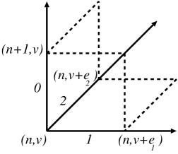
FIG. 1.: The elementary cell which we use to discretize BF theory.

The fundamental canonical variables of the theory are therefore $h^{k,I}_{n,v}$, $V^{I}_{n,v}$, $B^{k,a}_{n,v}$, $\lambda^{k}_{n,v}$ and $\mu_{n,v}$. The equations of motion for the variables $\lambda^{k}_{n,v}$ are,

$$\Pi^{\lambda^{k}}_{n+1,v} = \frac{\partial L(n,n+1)}{\partial\lambda^{k}_{n+1,v}}=0$$ (123)

$$\Pi^{\lambda^{k}}_{n,v} = -\frac{\partial L(n,n+1)}{\partial\lambda^{k}_{n,v}}=-{\rm Tr}\left[h^{k}_{n,v}\left(h^{k}_{n,v}\right)^{\dagger}-I\right]$$ (124)

Preservation in time of the primary constraint (123) leads to the secondary constraint

$${\rm Tr}\left[h^{k}_{n,v}\left(h^{k}_{n,v}\right)^{\dagger}-I\right]=0$$ (125)

and preserving in time this constraint does not yield any new constraints. The equations of motion for the variables $\mu_{n,v}$ are

$$\Pi^{\mu}_{n+1,v} = 0$$ (126)

$$\Pi^{\mu}_{n,v} = -{\rm Tr}\left[V_{n,v}\left(V_{n,v}\right)^{\dagger}-I\right].$$ (127)

Preserving in time constraints(126) leads to the constraints

$${\rm Tr}\left[V_{n,v}\left(V_{n,v}\right)^{\dagger}-I\right]=0$$ (128)

which is preserved in time without introducing any new constraints.

The equations of motion for the variables $B^{k,a}_{n,v}$ are

$$\Pi^{B^{k}}_{n+1,v} = \frac{\partial L(n,n+1)}{\partial B^{k,a}_{n+1,v}}\,\left(T^{a}\right)^{\dagger}=0$$ (129)

$$\Pi^{B^{k}}_{n,v} = -\frac{\partial L(n,n+1)}{\partial B^{k,a}_{n,v}}\,\left(T^{a}\right)^{\dagger}=-{\rm Tr}\left[h^{i\,j}_{n,v}\,T^{a}\right]\,\left(T^{a}\right)^{\dagger}$$ (130)

where $\{i,j,k\}$ is a cyclic permutation of $\{0,1,2\}$ and $h^{i\,j}_{n,v}$ is the holonomy starting from $n,v$ around the elementary plaquette in the plane $i-j$. Preserving in time the constraint (129) together with constraints (125,128) leads to

$$h^{i\,j}_{n,v}=\sigma^{i\,j}_{n,v}\,I$$ (131)

with $\sigma^{i\,j}_{n,v}=\pm 1$. This sign is arbitrary and can change from plaquette to plaquette.

The equations of motion for the variables $V^{I}_{n,v}$ are

$$\Pi^{V}_{n+1,v} = \frac{\partial L(n,n+1)}{\partial V^{I}_{n+1,v}}\,\left(T^{I}\right)^{\dagger}=0$$ (132)

$$V_{n,v}\Pi^{V}_{n,v} = h^{0\,1}_{n,v}B^{2}_{n,v}-h^{0\,2}_{n,v}B^{1}_{n,v}-\left(h^{1}_{n,v-e_{1}}\right)^{\dagger}h^{1\,0}_{n,v-e_{1}}B^{2}_{n,v-e_{1}}h^{1}_{n,v-e_{1}}$$ (134)

$$+\left(h^{2}_{n,v-e_{2}}\right)^{\dagger}h^{2\,0}_{n,v-e_{2}}B^{1}_{n,v-e_{2}}h^{2}_{n,v-e_{2}}+2\mu_{n,v}\,I\,.$$

Preserving in time the constraints (132), together with (131) leads to determining the multipliers

$$\mu_{n,v}=0$$ (135)

and the equation of motion,

$$h^{0\,1}_{n,v}B^{2}_{n,v}-h^{0\,2}_{n,v}B^{1}_{n,v}-\left(h^{1}_{n,v-e_{1}}\right)^{\dagger}h^{1\,0}_{n,v-e_{1}}B^{2}_{n,v-e_{1}}h^{1}_{n,v-e_{1}}+\left(h^{2}_{n,v-e_{2}}\right)^{\dagger}h^{2\,0}_{n,v-e_{2}}B^{1}_{n,v-e_{2}}h^{2}_{n,v-e_{2}}=0\,.$$ (136)

The equation of motion for $\Pi^{h^{1}}_{n+1,v}$ is

$$h^{1}_{n+1,v}\Pi^{h^{1}}_{n+1,v}=V^{\dagger}_{n,v}h^{0\,1}_{n,v}B^{2}_{n,v}V_{n,v}$$ (137)

and using (131) we obtain the primary constraint

$${\rm Tr}\left[h^{1}_{n+1,v}\Pi^{h^{1}}_{n+1,v}\right]=0\,.$$ (138)

Preserving in time this constraint, together with the equation of motion for $\Pi^{h^{1}}_{n,v}$ leads to the fixing the multiplier

$$\lambda^{1}_{n,v}=0$$ (139)

and the equation of motion

$$h^{1}_{n,v}\Pi^{h^{1}}_{n,v}=h^{1\,0}_{n,v}B^{2}_{n,v}-h^{1\,2}_{n,v}B^{0}_{n,v}+\left(h^{2}_{n,v-e_{2}}\right)^{\dagger}h^{2\,1}_{n,v-e_{2}}B^{0}_{n,v-e_{2}}h^{2}_{n,v-e_{2}}\,.$$ (140)

We proceed in a similar fashion for the variable $h^{2,I}_{n,v}$. The equations of motion lead to

$$h^{2}_{n+1,v}\Pi^{h^{2}}_{n+1,v} = -V^{\dagger}_{n,v}h^{0\,2}_{n,v}B^{1}_{n,v}V_{n,v}$$ (141)

$${\rm Tr}\left[h^{2}_{n+1,v}\Pi^{h^{2}}_{n+1,v}\right] = 0$$ (142)

$$\lambda^{2}_{n,v} = 0$$ (143)

$$h^{2}_{n,v}\Pi^{h^{2}}_{n,v} = h^{2\,1}_{n,v}B^{0}_{n,v}-h^{2\,0}_{n,v}B^{1}_{n,v}-\left(h^{1}_{n,v-e_{1}}\right)^{\dagger}h^{1\,2}_{n,v-e_{1}}B^{0}_{n,v-e_{1}}h^{1}_{n,v-e_{1}}\,.$$ (144)

We now consider the variable,

$$E^{k}_{n,v}\equiv h^{k}_{n,v}\Pi^{k}_{n,v}\quad k\in\{1,2\}\,,$$ (145)

that our experience with Yang–Mills shows should play the role of an electric field along the direction $e_{k}$ at the point $\{n,v\}$. Due to the constraints (138) y (142), the variable in question is an element of the algebra, i.e., is a traceless matrix,

$${\rm Tr}\left(E^{k}_{n,v}\right)=0.$$ (146)

We also define the electric field in the direction $-e_{k}$ at the point $\{n,v\}$ by

$$E^{\overline{k}}_{n,v}\equiv h^{\overline{k}}_{n,v}\Pi^{\overline{k}}_{n,v}=(h^{k}_{n,v-e_{k}})^{\dagger}(\Pi^{k}_{n,v-e_{k}})^{\dagger}=-(h^{k}_{n,v-e_{k}})^{\dagger}E^{k}_{n,v-e_{k}}h^{k}_{n,v-e_{k}}$$ (147)

Using the equations of motion and constraint it is straightforward to get

$$E^{1}_{n+1,v} = +V^{\dagger}_{n,v}h^{0\,1}_{n,v}B^{2}_{n,v}V_{n,v}$$ (148)

$$E^{2}_{n+1,v} = -V^{\dagger}_{n,v}h^{0\,2}_{n,v}B^{1}_{n,v}V_{n,v}$$ (149)

$$E^{\overline{1}}_{n+1,v} = -V^{\dagger}_{n,v}(h^{1}_{n,v-e_{1}})^{\dagger}h^{0\,1}_{n,v-e_{1}}B^{2}_{n,v-e_{1}}h^{1}_{n,v-e_{1}}V_{n,v}$$ (150)

$$E^{\overline{2}}_{n+1,v} = +V^{\dagger}_{n,v}(h^{2}_{n,v-e_{2}})^{\dagger}h^{0\,2}_{n,v-e_{2}}B^{1}_{n,v-e_{2}}h^{2}_{n,v-e_{2}}V_{n,v}$$ (151)

and from here one can show that (136) is equivalent to

$$E^{1}_{n+1,v}+E^{2}_{n+1,v}+E^{\overline{1}}_{n+1,v}+E^{\overline{2}}_{n+1,v}=0\,.$$ (152)

This is the familiar expression for Gauss’ law on the lattice.

We have noted that the holonomy along the plaquette $1-2$ is proportional to the identity. Therefore one is dealing with a flat connection on the plaquette. As expected, the discrete theory admits more solutions than the continuum one, in the sense that a possible solution would be a connection that makes the holonomy $+1$ on certain plaquettes and $-1$ on others. Such solutions will not admit a continuum counterpart.

We need to check that the Dirac brackets of the elementary variables lead to the expected results. Here we can just refer to the discussion we did in the Yang–Mills case, since the structure of the second class constraints (125,146) is similar to the one we encountered in that case.

The quantization of the theory is now immediate. The Dirac bracket between the electric field and the holonomy is similar to the one in the Maxwell case (96),

$$\left\{\left(E^{k}_{n,v}\right)^{A},h^{k}_{n,v}\right\}=iT^{A}h^{k}_{n,v}$$ (153)

where we have introduced the component notation in the algebra and the $T^{A}$’s are the generators of $su(2)$ we introduced before.

One can now consider wavefunctions that are functions of the holonomies on the links of the lattice, $\Psi[h^{k}_{n,v}]$. Following the Dirac method we need to impose the constraints as operator equations. Gauss’ law will just state that the wavefunctions are gauge invariant. In this case it will imply that the wavefunctions are linear combinations of traces of holonomies along closed loops.

We now need to impose the spatial projection of the constraint (131) as an operatorial equation,

$$h^{1\,2}_{n,v}=\sigma^{1\,2}_{n,v}\,I.$$ (154)

In the space of functions of holonomies the equation becomes multiplicative and the solution is that the holonomies along all elementary plaquettes should be $\pm 1$ times the identity. We therefore see that we recover as solutions of the theory the space of gauge invariant functions of a flat connection. Except that in the discrete theory it could happen that in some plaquettes the holonomies are $+1$ times the identity whereas in others the holonomies have a negative sign. Such solutions are possible in the discrete theory and do not have a counterpart in the continuum. We see that the discrete theory therefore has considerably richer solution structure than the continuum theory. If one however imposes that the solutions be continuous from one plaquette to another, one is only left with the traditional solution.

The unitary operator that implements the finite canonical transformation is, for this theory, given by an exponential of a combination of the first class constraints with arbitrary coefficients.

V Conclusions

We have generalized classical mechanics to systems in which space and time are discrete. Time evolution is implemented through a finite canonical transformation. Constrained systems can be incorporated in the scheme. We discussed in detail how to handle Yang–Mills theory, Maxwell theory and BF theory and encountered no problem setting up the classical and quantum theory. In general, the discrete theories contain many solutions that do not have a good continuum limit, as we have seen in the BF example, and the correct solution has to be chosen by requesting that it have the appropriate semiclassical limit.

The framework we have set up is completely ready to be applied to the case of general relativity, which will have many similarities with the BF case. An attractive advantage is that the formalism does not require an Euclidean rotation and operates directly in terms of the Lorentzian signature theory. We will discuss the case of general relativity in a forthcoming publication. Having a sound theoretical foundation for dealing with discretized gravity will allow quantize the theory in a systematic way and will enable us to make connections between the canonical and path integral approaches.

- [1] M. Choptuik, Phys. Rev. D44, 3124 (1991).
- [2] M. Bander, Phys. Rev. D36, 2297 (1987); 38, 1056 (1988).
- [3] J. L. Friedman and I. Jack, J. Math. Phys. 27, 2973 (1986).
- [4] T. Thiemann, Class. Quan. Grav. 15 839; 875; 1207; 1249; 1281; 1463 (1998)
- [5] J. Lewandowski, D. Marolf, Int. J. Mod. Phys. D7, 299 (1998); R. Gambini, J. Lewandowski, D. Marolf, J. Pullin, Int. J. Mod. Phys. D7 97 (1997).
- [6] L. Smolin gr-qc/9609034.
- [7] D. Neville Phys. Rev. D59, 044032 (1999)
- [8] M. Henneaux, C. Teitelboim, “Quantization of gauge systems”, Princeton University Press, Princeton, NJ (1992).
- [9] R. Loll, Liv. Rev. Relat. 1, 13 (1998).
- [10] S. Kauffman and L. Smolin, Lect. Notes Phys. 541, 101 (2000).
- [11] J. Baez, J. Gilliam, Lett. Math. Phys. 31, 205 (1994).
- [12] T. D. Lee, in “How far are we from the gauge forces” Antonino Zichichi, ed. Plenum Press, (1985)
- [13] S. Maeda, Math. Japonica 26, 85 (1981).
- [14] J. Logan, Aequat. Math. 9, 210 (1973).
- [15] G. Jaroszkiewicz, K. Norton, J. Phys. A30, 3115 (1997).
- [16] See for instance, J. Marsden, W. Shadwick, G. Patrick “Integration algorithms and classical mechanics”, American Mathematical Society, Bloomington, (1996) or D. Markiewicz, “Survey of symplectic integrators”, http://www.math.berkeley.edu/ alanw/242papers99.html.
- [17] M. Preto, S. Tremaine, astro-ph/9906322.
- [18] H. Goldstein, “Classical Mechanics”, Addison Wesley, Don Mills, Ontario (1980).
- [19] J. José, E. Saletan, “Classical dynamics, a contemporary approach”, Cambridge University Press, Cambridge (1998).
- [20] P. Renteln, L. Smolin, Class. Quant. Grav. 6, 275 (1989).
- [21] M. Creutz, Phys. Rev. D 15, 1128 (1977).
- [22] P. Menotti, A. Pelissetto, Phys. Rev. D35, 1194 (1987).