Detection template families for gravitational waves from the final stages of binary–black-hole inspirals: Nonspinning case

Abstract

We investigate the problem of detecting gravitational waves from binaries of nonspinning black holes with masses $m=5\mbox{--}20M_{\odot}$, moving on quasicircular orbits, which are arguably the most promising sources for first-generation ground-based detectors. We analyze and compare all the currently available post–Newtonian approximations for the relativistic two-body dynamics; for these binaries, different approximations predict different waveforms. We then construct examples of detection template families that embed all the approximate models, and that could be used to detect the true gravitational-wave signal (but not to characterize accurately its physical parameters). We estimate that the fitting factor for our detection families is $\gtrsim 0.95$ (corresponding to an event-rate loss $\lesssim 15$%) and we estimate that the discretization of the template family, for $\sim 10^{4}$ templates, increases the loss to $\lesssim 20$%.

I Introduction

A network of broadband ground-based laser interferometers, aimed at detecting gravitational waves (GWs) in the frequency band 10–10³ Hz, is currently beginning operation and, hopefully, will start the first science runs within this year (2002). This network consists of the British–German GEO, the American Laser Interferometer Gravitational-wave Observatory (LIGO), the Japanese TAMA and the Italian–French VIRGO (which will begin operating in 2004) Inter .

The first detection of gravitational waves with LIGO and VIRGO interferometers is likely to come from binary black-hole systems where each black hole has a mass  of a few $M_{\odot}$, and the total mass is roughly in the range $10\mbox{--}40M_{\odot}$ FK , and where the orbit is quasicircular (it is generally assumed that gravitational radiation reaction will circularize the orbit by the time the binary is close to the final coalescence LW ). It is easy to see why. Assuming for simplicity that the GW signal comes from a quadrupole-governed, Newtonian inspiral that ends at a frequency outside the range of good interferometer sensitivity, the signal-to-noise ratio S/N is $\propto{\cal M}^{5/6}/d$ (See, e.g., Ref. KT300 ), where ${\cal M}=M\eta^{3/5}$ is the chirp mass (with $M=m_{1}+m_{2}$ the total mass and $\eta=m_{1}m_{2}/M^{2}$), and $d$ is the distance between the binary and the Earth. Therefore, for a given signal-to-noise detection threshold (see Sec. II) and for equal-mass binaries ($\eta=1/4$), the larger is the total mass, the larger is the distance $d$ that we are able to probe. [In Sec. V we shall see how this result is modified when we relax the assumption that the signal ends outside the range of good interferometer sensitivity.]

For example, a black-hole–black hole binary (BBH) of total mass $M=20M_{\odot}$ at 100 Mpc gives (roughly) the same S/N as a neutron-star–neutron-star binary (BNS) of total mass $M=2.8M_{\odot}$ at 20 Mpc. The expected measured-event rate scales as the third power of the probed distance, although of course it depends also on the system’s coalescence rate per unit volume in the universe. To give some figures, computed using LIGO-I’s sensitivity specifications, if we assume that BBHs originate from main-sequence binaries postnov , the estimated detection rate per year is $\lesssim\,4\times 10^{-3}\mbox{--}0.6$ at $100\,{\rm Mpc}$ KNST ; KT , while if globular clusters are considered as incubators of BBHs PZ99 the estimated detection rate per year is $\sim 0.04\mbox{--}0.6$ at $100\,{\rm Mpc}$ KNST ; KT ; by contrast, the BNS detection rate per year is in the range $3\times 10^{-4}\mbox{--}0.3$ at $20\,{\rm Mpc}$ KNST ; KT . The very large cited ranges for the measured-event rates reflect the uncertainty implicit in using population-synthesis techniques and extrapolations from the few known galactic BNSs to evaluate the coalescence rates of binary systems. [In a recent article Miller , Miller and Hamilton suggest that four-body effects in globular clusters might enhance considerably the BBH coalescence rate, brightening the prospects for detection with first-generation interferometers; the BBHs involved might have relatively high BH masses ($\sim 100M_{\odot}$) and eccentric orbits, and they will not be considered in this paper.]

The GW signals from standard comparable-mass BBHs with $M=10\mbox{--}40M_{\odot}$ contain only few ($50\mbox{--}800$) cycles in the LIGO–VIRGO frequency band, so we might expect that the task of modeling the signals for the purpose of data analysis could be accomplished easily. However, the frequencies of best interferometer sensitivity correspond to GWs emitted during the final stages of the inspiral, where the post–Newtonian (PN) expansion PN , which for compact bodies is essentially an expansion in the characteristic orbital velocity $v/c$, begins to fail. It follows that these sources require a very careful analysis. As the two bodies draw closer, and enter the nonlinear, strong-curvature phase, the motion becomes relativistic, and it becomes harder and harder to extract reliable information from the PN series. For example, using the Keplerian formula $v=(\pi Mf_{\rm GW})^{1/3}$ [where $f_{\mathrm{GW}}$ is the GW frequency] and taking $f_{\rm GW}=153$ Hz [the LIGO-I peak-sensitivity frequency] we get $v(M)=0.14(M/M_{\odot})^{1/3}$; hence, for BNSs $v(2.8M_{\odot})=0.2$, but for BBHs $v(20M_{\odot})=0.38$ and $v(40M_{\odot})=0.48$.

The final phase of the inspiral (at least when BH spins are negligible) includes the transition from the adiabatic inspiral to the plunge, beyond which the motion of the bodies is driven (almost) only by the conservative part of the dynamics. Beyond the plunge, the two BHs merge, forming a single rotating BH in a very excited state; this BH then eases into its final stationary Kerr state, as the oscillations of its quasinormal modes die out. In this phase the gravitational signal will be a superposition of exponentially damped sinusoids (ringdown waveform). For nonspinning BBHs, the plunge starts roughly at the innermost stable circular orbit (ISCO) of the BBH. At the ISCO, the GW frequency [evaluated in the Schwarzschild test-mass limit as $f_{\rm GW}^{\rm ISCO}(M)\simeq 0.022/M$] is $f_{\rm GW}^{\rm ISCO}(20M_{\odot})\simeq 220\,{\rm Hz}$ and $f_{\rm GW}^{\rm ISCO}(30M_{\odot})\simeq 167\,{\rm Hz}$. These frequencies are well inside the LIGO and VIRGO bands.

The data analysis of inspiral, merger (or plunge), and ringdown of compact binaries was first investigated by Flanagan and Hughes FH , and more recently by Damour, Iyer and Sathyaprakash DIS3 . Flanagan and Hughes FH model the inspiral using the standard quadrupole prediction (see, e.g., Ref. KT300 ), and assume an ending frequency of $0.02/M$ (the point where, they argue, PN and numerical-relativity predictions start to deviate by $\sim 5\%$ C ). They then use a crude argument to estimate upper limits for the total energy radiated in the merger phase ($\sim 0.1M$) and in the ringdown phase ($\sim 0.03M$) of maximally-spinning–BBH coalescences. Damour, Iyer and Sathyaprakash DIS3 study the nonadiabatic PN-resummed model for non spinning BBHs of Refs. BD1 ; BD2 ; EOB3PN , where the plunge can be seen as a natural continuation of the inspiral BD2 rather than a separate phase; the total radiated energy is $0.007M$ in the merger and $0.007M$ in the ringdown BD3 . (All these values for the energy should be also compared with the value, $0.025\mbox{--}0.03M$, estimated recently in Ref. BBCLT01 for the plunge and ringdown for non spinning BBHs.) When we deal with nonadiabatic models, we too shall choose not to separate the various phases. Moreover, because the ringdown phase does not give a significant contribution to the signal-to-noise ratio for $M\leq 200M_{\odot}$ FH ; DIS3 , we shall not include it in our investigations.

BHs could have large spins: various studies kidder ; apostolatos have shown that when this is the case, the time evolution of the GW phase and amplitude during the inspiral will be significantly affected by spin-induced modulations and irregularities. These effects can become dramatic, if the two BH spins are large and are not aligned or antialigned with the orbital angular momentum. There is a considerable chance that the analysis of interferometer data, carried out without taking into account spin effects, could miss the signals from spinning BBHs altogether. We shall tackle the crucial issue of spin in a separate paper BCV .

The purpose of the present paper is to discuss the problem of the failure of the PN expansion during the last stages of inspiral for nonspinning BHs, and the possible ways to deal with this failure. This problem is known in the literature as the intermediate binary black hole (IBBH) problem BCT . Despite the considerable progress made by the numerical-relativity community in recent years C ; TB ; PTC ; GGB , a reliable estimate of the waveforms emitted by BBHs is still some time ahead (some results for the plunge and ringdown waveforms were obtained very recently BBCLT01 , but they are not very useful for our purposes, because they do not include the last stages of the inspiral before the plunge, and their initial data are endowed with large amounts of spurious GWs). To tackle the delicate issue of the late orbital evolution of BBHs, various nonperturbative analytical approaches to that evolution (also known as PN resummation methods) have been proposed DIS1 ; BD1 ; BD2 ; EOB3PN .

The main features of PN resummation methods can be summarized as follows: (i) they provide an analytic (gauge-invariant) resummation of the orbital energy function and gravitational flux function (which, as we shall see in Sec. III, are the two crucial ingredients to compute the gravitational waveforms in the adiabatic limit); (ii) they can describe the motion of the bodies (and provide the gravitational waveform) beyond the adiabatic approximation; and (iii) in principle they can be extended to higher PN orders. More importantly, they can provide initial dynamical data for the two BHs at the beginning of the plunge (such as their positions and momenta), which can be used (in principle) in numerical relativity to help build the initial gravitational data (the metric and its time derivative) and then to evolve the full Einstein equations through the merger phase. However, these resummation methods are based on some assumptions that, although plausible, have not been proved: for example, when the orbital energy and the gravitational flux functions are derived in the comparable-mass case, it is assumed that they are smooth deformations of the analogous quantities in the test-mass limit. Moreover, in the absence of both exact solutions and experimental data, we can test the robustness and reliability of the resummation methods only by internal convergence tests.

In this paper we follow a more conservative point of view. We shall maintain skepticism about waveforms emitted by BBH with $M=10\mbox{--}40M_{\odot}$ and evaluated from PN calculations, as well as all other waveforms ever computed for the late BBH inspiral and plunge, and we shall develop families of search templates that incorporate this skepticism. More specifically, we shall be concerned only with detecting BBH GWs, and not with extracting physical parameters, such as masses and spins, from the measured GWs. The rationale for this choice is twofold. First, detection is the more urgent problem at a time when GW interferometers are about to start their science runs; second, a viable detection strategy must be constrained by the computing power available to process a very long stream of data, while the study of detected signals to evaluate physical parameters can concentrate many resources on a small stretch of detector output. In addition, as we shall see in Sec. VI, and briefly discuss in Sec. VI.4, the different PN methods will give different parameter estimations for the same waveform, making a full parameter extraction fundamentally difficult.

This is the strategy that we propose: we guess (and hope) that the conjunction of the waveforms from all the post–Newtonian models computed to date spans a region in signal space that includes (or almost includes) the true signal. We then choose a detection (or effective) template family that approximates very well all the PN expanded and resummed models (henceforth denoted as target models). If our guess is correct, the effectualness DIS1 of the effective model in approximating the targets (i.e., its capability of reproducing their signal shapes) should be indicative of its effectualness in approximating the true signals. Because our goal is the detection of BBH GWs, we shall not require the detection template family to be faithful DIS1 (i.e., to have a small bias in the estimation of the masses).

As a backup strategy, we require the detection template family to embed the targets in a signal space of higher dimension (i.e., with more parameters), trying to guess the functional directions in which the true signals might lie with respect to the targets (of course, this guess is rather delicate!). So, the detection template families constructed in this paper cannot be guaranteed to capture the true signal, but they should be considered as indications.

This paper is organized as follows. In Sec. II, we briefly review the theory of matched-filtering GW detections, which underlies the searches for GWs from inspiraling binaries. Then in Secs. III, IV, and V we present the target models and give a detailed analysis of the differences between them, both from the point of view of the orbital dynamics and of the gravitational waveforms. More specifically, in Sec. III we introduce the two-body adiabatic models, both PN expanded and resummed; in Sec. IV we introduce nonadiabatic approximations to the two-body dynamics; and in Sec. V we discuss the signal-to-noise ratios obtained for the various two-body models. Our proposals for the detection template families are discussed in the Fourier domain in Sec. VI, and in the time domain in Sec. VII, where we also build the mismatch metric Sub ; O for the template banks and use it to evaluate the number of templates needed for detection. Section VIII summarizes our conclusions.

Throughout this paper we adopt the LIGO noise curve given in Fig. 1 and Eq. (28), and used also in Ref. DIS3 . Because the noise curve anticipated for VIRGO [see Fig. 1] is quite different (both at low frequencies, and in the location of its peak-sensitivity frequency) our results cannot be applied naively to VIRGO. We plan to repeat our study for VIRGO in the near future.

II The theory of matched-filtering signal detection

The technique of matched-filtering detection for GW signals is based on the systematic comparison of the measured detector output ${s}$ with a bank of theoretical signal templates $\{{u_{i}}\}$ that represent a good approximation to the class of physical signals that we seek to measure. This theory was developed by many authors over the years, who have published excellent expositions Finn ; Finnchernoff ; Wainstein ; DIS1 ; O ; FH ; Davis ; Oppenheim ; Hancock ; Cutlerflanagan ; SatDhu1 ; SatDhu2 ; Sathya ; DIS2 . In the following, we summarize the main results and equations that are relevant to our purposes, and we establish our notation.

II.1 The statistical theory of signal detection

The detector output ${s}$ consists of noise ${n}$ and possibly of a true gravitational signal ${h_{i}}$ (part of a family $\{{h_{i}}\}$ of signals generated by different sources for different source parameters, detector orientations, and so on). Although we may be able to characterize the properties of the noise in several ways, each separate realization of the noise is unpredictable, and it might in principle fool us by hiding a physical signal (hence the risk of a false dismissal) or by simulating one (false alarm). Thus, the problem of signal detection is essentially probabilistic. In principle, we could try to evaluate the conditional probability $P(h|s)$ that the measured signal $s$ actually contains one of the $h_{i}$. In practice, this is inconvenient, because the evaluation of $P(h|s)$ requires the knowledge of the a priori probability that a signal belonging to the family $\{h_{i}\}$ is present in $s$.

What we can do, instead, is to work with a statistic (a functional of $s$ and of the $h_{i}$) that (for different realizations of the noise) will be distributed around low values if the physical signal ${h_{i}}$ is absent, and around high value if the signal is present. Thus, we shall establish a decision rule as follows Wainstein : we will claim a detection if the value of a statistic (for a given instance of ${s}$ and for a specific ${h_{i}}$) is higher than a predefined threshold. We can then study the probability distribution of the statistic to estimate the probability of false alarm and of false dismissal. The steps involved in this statistical study are easily laid down for a generic model of noise, but it is only in the much simplified case of normal noise that it is possible to obtain manageable formulas; and while noise will definitely not be normal in a real detector, the Gaussian formulas can still provide useful guidelines for the detection problems. Eventually, the statistical analysis of detector search runs will be carried out with numerical Montecarlo techniques that make use of the measured characteristics of the noise. So throughout this paper we shall always assume Gaussian noise.

The statistic that is generally used is based on the symmetric inner product ${\langle g,h\rangle}$ between two real signals ${g}$ and ${h}$, which represents essentially the cross-correlation between $g$ and $h$, weighted to emphasize the correlation at the frequencies where the detector sensitivity is better. We follow Cutler and Flanagan’s conventions Cutlerflanagan and define

$${\langle g,h\rangle}=2\int_{-\infty}^{+\infty}\frac{\tilde{g}^{*}(f)\tilde{h}(f)}{S_{n}(|f|)}df=4\,\mathrm{Re}\int_{0}^{+\infty}\frac{\tilde{g}^{*}(f)\tilde{h}(f)}{S_{n}(f)}df,$$ (1)

where $S_{n}(f)$, the one-sided noise power spectral density, is given by

$$\overline{\tilde{n}^{*}(f_{1})\tilde{n}(f_{2})}=\frac{1}{2}\delta(f_{1}-f_{2})S_{n}(f_{1})\quad\mbox{for $f_{1}>0$},$$ (2)

and $S_{n}(f_{1})=0$ for $f_{1}<0$. We then define the signal-to-noise ratio $\rho$ (for the measured signal ${s}$ after filtering by ${h_{i}}$), as

$$\rho(h_{i})=\frac{{\langle s,h_{i}\rangle}}{\mathrm{rms}\,{\langle n,h_{i}\rangle}}=\frac{{\langle s,h_{i}\rangle}}{\sqrt{{\langle h_{i},h_{i}\rangle}}},$$ (3)

where the equality follows because $\overline{{\langle h_{i},n\rangle}{\langle n,h_{i}\rangle}}={\langle h_{i},h_{i}\rangle}$ (see, e.g., Wainstein ). In the case of Gaussian noise, it can be proved that this filtering technique is optimal, in the sense that it maximizes the probability of correct detection for a given probability of false detection.

In the case when ${s}={n}$, and when noise is Gaussian, it is easy to prove that $\rho$ is a normal variable with a mean of zero and a variance of one. If instead ${s}={h_{i}}+{n}$, then $\rho$ is a normal variable with mean $\sqrt{{\langle h_{i},h_{i}\rangle}}$ and unit variance. The threshold $\rho_{*}$ for detection is set as a tradeoff between the resulting false-alarm probability,

$$\mathcal{F}=\sqrt{\frac{1}{2\pi}}\int_{\rho_{*}}^{+\infty}e^{-\rho^{2}/2}d\rho=\frac{1}{2}\mathrm{erfc}\,(\rho_{*}/\sqrt{2})$$ (4)

(where $\mathrm{erfc}$ is the complementary error function Abramowitz ), and the probability of correct detection

$$\mathcal{D}=\frac{1}{2}\mathrm{erfc}\,[(\rho_{*}-\sqrt{{\langle h_{i},h_{i}\rangle}})/\sqrt{2}]$$ (5)

(the probability of false dismissal is just $1-\mathcal{D}$).

II.2 Template families and extrinsic parameters

We can now go back to the initial strategy of comparing the measured signal against a bank of $\mathcal{N}_{i}$ templates $\{{u_{i}}\}$ that represent a plurality of sources of different types and physical parameters. For each stretch ${s}$ of detector output, we shall compute the signal-to-noise ratio ${\langle s,u_{i}\rangle}/\sqrt{{\langle u_{i},u_{i}\rangle}}$ for all the ${u_{i}}$, and then apply our rule to decide whether the physical signal corresponding to any one of the ${u_{i}}$ is actually present within ${s}$ KT300 . Of course, the threshold $\rho_{*}$ needs to be adjusted so that the probability $\mathcal{F}_{\mathrm{tot}}$ of false alarm over all the templates is still acceptable. Under the assumption that all the inner products ${\langle n,u_{i}\rangle}$ of the templates with noise alone are statistically independent variables [this hypothesis entails ${\langle u_{i},u_{j}\rangle}\simeq 0$], $\mathcal{F}_{\mathrm{tot}}$ is just $1-(1-\mathcal{F})^{\mathcal{N}_{i}}\sim\mathcal{N}_{i}\mathcal{F}$. If the templates are not statistically independent, this number is an upper limit on the false alarm rate. However, we first need to note that, for any template ${u_{i}}$, there are a few obvious ways (parametrized by the so-called extrinsic parameters) of changing the signal shape that do not warrant the inclusion of the modified signals as separate templates

The extrinsic parameters are the signal amplitude, phase and time of arrival. Any true signal ${h}$ can be written in all generality as

$$h(t)=\mathcal{A}_{h}a_{h}[t-t_{h}]\cos[\Phi_{h}(t-t_{h})+\phi_{h}],$$ (6)

where $a_{h}(t)=0$ for $t<0$, where $\Phi_{h}(0)=0$, and where $a_{h}(t)$ is normalized so that ${\langle h,h\rangle}=\mathcal{A}_{h}^{2}$. While the template bank $\{{u_{i}}\}$ must contain signal shapes that represent all the physically possible functional forms $a(t)$ and $\Phi(t)$, it is possible to modify our search strategy so that the variability in $\mathcal{A}_{h}$, $\phi_{h}$ and $t_{h}$ is automatically taken into account without creating additional templates.

The signal amplitude is the simplest extrinsic parameter. It is expedient to normalize the templates ${u_{i}}$ so that ${\langle u_{i},u_{i}\rangle}=1$, and $\rho({u_{i}})={\langle s,u_{i}\rangle}$. Indeed, throughout the rest of this paper we shall always assume normalized templates. If ${s}$ contains a scaled version $h_{i}=\mathcal{A}u_{i}$ of a template ${u_{i}}$ (here $\mathcal{A}$ is known as the signal strength), then $\overline{\rho(u_{i})}=\mathcal{A}$. However, the statistical distribution of $\rho$ is the same in the absence of the signal. Then the problem of detection signals of known shape and unknown amplitude is easily solved by using a single normalized template and the same threshold $\rho_{*}$ as used for the detection of completely known signals Wainstein . Quite simply, the stronger an actual signal, the easier it will be to reach the threshold.

We now look at phase, and we try to match ${h}$ with a continuous one-parameter subfamily of templates $u(\phi_{t};t)=a_{h}(t)\cos[\Phi_{h}(t)+\phi_{t}]$. It turns out that for each time signal shape $\{a(t),\Phi(t)\}$, we need to keep in our template bank only two copies of the corresponding ${u_{i}}$, for $\phi_{t}=0$ and $\phi_{t}=\pi/2$, and that the signal to noise of the detector output ${s}$ against ${u_{i}}$, for the best possible value of $\phi_{t}$, is automatically found as Wainstein

$$\rho_{\phi}=\max_{\phi_{t}}{\langle s,u_{i}(\phi_{t})\rangle}=\sqrt{\left|{\langle s,u_{i}(0)\rangle}\right|^{2}+\left|{\langle s,u_{i}(\pi/2)\rangle}\right|^{2}}\,,$$ (7)

where $u_{i}(0)$ and $u_{i}(\pi/2)$ have been orthonormalized. The statistical distribution of the phase-maximized statistic $\rho_{\phi}$, for the case of (normal) noise alone, is the Raleigh distribution Wainstein

$$p_{0}(\rho_{\phi})=\rho_{\phi}e^{-\rho_{\phi}^{2}/2},$$ (8)

and the false-alarm probability for a threshold $\rho_{\phi*}$ is just

$$\mathcal{F}=e^{-\rho_{\phi*}^{2}/2}.$$ (9)

Throughout this paper, we will find it useful to consider inner products that are maximized (or minimized) with respect to the phases of both templates and reference signals. In particular, we shall follow Damour, Iyer and Sathyaprakash in making a distinction between the best match or maxmax match

$$\mathrm{maxmax}{\langle h,u_{i}\rangle}=\max_{\phi_{h}}\max_{\phi_{t}}{\langle h(\phi_{h}),u_{i}(\phi_{t})\rangle},$$ (10)

which represents the most favorable combination of phases between the signals ${h}$ and ${u_{i}}$, and the minmax match

$$\mathrm{minmax}{\langle h,u_{i}\rangle}=\min_{\phi_{h}}\max_{\phi_{t}}{\langle h(\phi_{h}),u_{i}(\phi_{t})\rangle},$$ (11)

which represents the safest estimate in the realistic situation, where we cannot choose the phase of the physical measured signal, but only of the template used to match the signal. Damour, Iyer and Sathyaprakash [see Appendix B of Ref. DIS1 ] show that both quantities are easily computed as

$$\left(\begin{array}[]{c}\mathrm{maxmax}\\ \mathrm{minmax}\end{array}\right)=\left\{\frac{A+B}{2}\pm\left[\left(\frac{A-B}{2}\right)^{2}+C^{2}\right]^{1/2}\right\}^{1/2},$$ (12)

where

$$A = {\langle h(0),u_{i}(0)\rangle}^{2}+{\langle h(0),u_{i}(\pi/2)\rangle}^{2},$$ (13)

$$B = {\langle h(\pi/2),u_{i}(0)\rangle}^{2}+{\langle h(\pi/2),u_{i}(\pi/2)\rangle}^{2},$$ (14)

$$C = {\langle h(0),u_{i}(0)\rangle}{\langle h(\pi/2),u_{i}(0)\rangle}+$$

$${\langle h(0),u_{i}(\pi/2)\rangle}{\langle h(\pi/2),u_{i}(\pi/2)\rangle}.$$

In these formulas we have assumed that the two bases $\{{h(0)},{h(\pi/2)}\}$ and $\{{u_{i}(0)},{u_{i}(\pi/2)}\}$ have been orthonormalized.

The time of arrival $t_{h}$ is an extrinsic parameter because the signal to noise for the normalized, time-shifted template ${u(t-t_{0})}$ against the signal ${s}$ is just

$${\langle s,u(t_{0})\rangle}=4\,\mathrm{Re}\int_{0}^{+\infty}\frac{\tilde{s}^{*}(f)\tilde{u}(f)}{S_{n}(f)}e^{i2\pi ft_{0}}df,$$ (16)

where we have used a well-known property of the Fourier transform of time-shifted signals. These integrals can be computed at the same time for all the time of arrivals $\{t_{0}\}$, using a fast Fourier transform technique that requires $\sim N_{s}\log N_{s}$ operations (where $N_{s}$ is the number of the samples that describe the signals) as opposed to $\sim N_{s}^{2}$ required to compute all the integrals separately Schutz . Then we can look for the optimal $t_{0}$ that yields the maximum signal to noise.

We now go back to adjusting the threshold $\rho_{*}$ for a search over a vast template bank, using the estimate (9) for the false-alarm probability. Assuming that the statistics $\rho_{\phi}$ for each signal shape and starting time are independent, we require that

$$e^{-\rho_{\phi*}^{2}/2}\simeq\frac{\mathcal{F}_{\mathrm{tot}}}{N_{\mathrm{times}}N_{\mathrm{shapes}}},$$ (17)

or

$$\rho_{*}\simeq\sqrt{2(\log N_{\mathrm{times}}+\log N_{\mathrm{shapes}}-\log\mathcal{F}_{\mathrm{tot}})}.$$ (18)

It is generally assumed that $N_{\mathrm{times}}\sim 3\times 10^{10}$ (equivalent to templates displaced by 0.01 s over one year Cutler ; FH ) and that the false-alarm probability $\mathcal{F}_{\mathrm{tot}}\sim 10^{-3}$. Using these values, we find that an increase of $\rho_{*}$ by about $\sim 3\%$ is needed each time we increase $N_{\mathrm{shapes}}$ by one order of magnitude. So there is a tradeoff between the improvement in signal-to-noise ratio obtained by using more signal shapes and the corresponding increase in the detection threshold for a fixed false-alarm probability.

II.3 Imperfect detection and discrete families of templates

There are two distinct reasons why the detection of a physical signal ${h}$ by matched filtering with a template bank $\{{u_{i}}\}$ might result in signal-to-noise ratios lower than the optimal signal-to-noise ratio,

$$\rho_{\mathrm{opt}}=\sqrt{{\langle h,h\rangle}}.$$ (19)

First, the templates, understood as a continuous family $\{u(\lambda^{A})\}$ of functional shapes indexed by one or more intrinsic parameters $\lambda^{A}$ (such as the masses, spins, etc.), might give an unfaithful representation of ${h}$, introducing errors in the representation of the phasing or the amplitude. The loss of signal to noise due to unfaithful templates is quantified by the fitting factor $\mathrm{FF}$, introduced by Apostolatos ApostolatosFF , and defined by

$$\mathrm{FF}({h},{u(\lambda^{A})})=\frac{\max_{\lambda^{A}}{\langle h,u(\lambda^{A})\rangle}}{\sqrt{{\langle h,h\rangle}}}.$$ (20)

In general, we will be interested in the FF of the continuous template bank in representing a family of physical signals $\{{h(\theta^{A})}\}$, dependent upon one or more physical parameters $\theta^{A}$: so we shall write $\mathrm{FF}(\theta^{A})=\mathrm{FF}({h(\theta^{A})},{u(\lambda^{A})})$. Although it is convenient to index the template family by the same physical parameters $\theta^{A}$ that characterize ${h(\theta^{A})}$, this is by no means necessary; the template parameters $\lambda^{A}$ might be a different number than the physical parameters (indeed, this is desirable when the $\theta^{A}$ get to be very many), and they might not carry any direct physical meaning. Notice also that the value of the $\mathrm{FF}$ will depend on the parameter range chosen to maximize the $\lambda^{A}$.

The second reason why the signal-to-noise will be degraded with respect to its optimal value is that, even if our templates are perfect representations of the physical signals, in practice we will not adopt a continuous family of templates, but we will be limited to using a discrete bank $\{{u_{i}}\equiv{u(\lambda^{A}_{i})}\}$. This loss of signal to noise depends on how finely templates are laid down over parameter space SatDhu1 ; SatDhu2 ; Sathya ; a notion of metric in template space (the mismatch metric O ; Sub ; SO ) can be used to guide the disposition of templates so that the loss (in the perfect-template abstraction) is limited to a fixed, predetermined value, the minimum match $\mathrm{MM}$, introduced in Refs. SatDhu1 ; O , and defined by

$$\mathrm{MM}=\min_{\hat{\lambda}^{A}}\max_{\lambda^{A}_{i}}{\langle u(\hat{\lambda}^{A}),u(\lambda^{A}_{i})\rangle}=\min_{\hat{\lambda}^{A}}\max_{\Delta\lambda^{A}_{i}}{\langle u(\hat{\lambda}^{A}),u(\hat{\lambda}^{A}+\Delta\lambda^{A}_{i})\rangle},$$ (21)

where $\Delta\lambda^{A}_{i}\equiv\lambda^{A}_{i}-\hat{\lambda}^{A}$. The mismatch metric $g_{BC}(\hat{\lambda}^{A})$ for the template space $\{u(\lambda^{A})\}$ is obtained by expanding the inner product (or match) ${\langle u(\hat{\lambda}^{A}),u(\hat{\lambda}^{A}+\Delta\lambda^{A})\rangle}$ about its maximum of 1 at $\Delta\lambda^{A}=0$:

$${\langle u(\hat{\lambda}^{A}),u(\hat{\lambda}^{A}+\Delta\lambda^{A})\rangle}=M(\hat{\lambda}^{A},\hat{\lambda}^{A}+\Delta\lambda^{A})=1+\frac{1}{2}\left.\frac{\partial^{2}M}{\partial\Delta\lambda^{B}\partial\Delta\lambda^{C}}\right|_{\hat{\lambda}^{A}}\Delta\lambda^{B}\Delta\lambda^{C}+\,\cdots,$$ (22)

so the mismatch $1-\mathrm{M}$ between ${u(\hat{\lambda}^{A})}$ and the nearby template ${u(\hat{\lambda}^{A}+\Delta\lambda^{A})}$ can be seen as the square of the proper distance in a differential manifold indexed by the coordinates $\lambda^{A}$ O ,

$$1-M(\hat{\lambda}^{A},\hat{\lambda}^{A}+\Delta\lambda^{A})=g_{BC}\Delta\lambda^{B}\Delta\lambda^{C},$$ (23)

where

$$g_{BC}=-\frac{1}{2}\left.\frac{\partial^{2}M}{\partial\Delta\lambda^{B}\partial\Delta\lambda^{C}}\right|_{\hat{\lambda}^{A}}.$$ (24)

If, for simplicity, we lay down the $n$-dimensional discrete template bank $\{{u(\lambda^{A}_{i})}\}$ along a hypercubical grid of cellsize $dl$ in the metric $g_{AB}$ (a grid in which all the templates on nearby corners have a mismatch of $dl$ with each other), the minimum match occurs when $\hat{\lambda}^{A}$ lies exactly at the center of one of the hypercubes: then $1-\mathrm{MM}=n(dl/2)^{2}$. Conversely, given MM, the volume of the corresponding hypercubes is given by $V_{\mathrm{MM}}=(2\sqrt{(1-\mathrm{MM})/n})^{n}$. The number of templates required to achieve a certain MM is obtained by integrating the proper volume of parameter space within the region of physical interest, and then dividing by $V_{\mathrm{MM}}$:

$$\mathcal{N}[g,\mathrm{MM}]=\frac{\int\sqrt{|g|}d\lambda^{A}}{\left(2\sqrt{[1-\mathrm{MM}]/n}\right)^{n}}.$$ (25)

In practice, if the metric is not constant over parameter space it will not be possible to lay down the templates on an exact hypercubical grid of cellsize $dl$, so $\mathcal{N}$ will be somewhat higher than predicted by Eq. (25). However, we estimate that this number should be correct within a factor of two, which is adequate for our purposes.

In the worst possible case, the combined effect of unfaithful modeling ($\mathrm{FF}<1$) and discrete template family ($\mathrm{MM}<1$) will degrade the optimal signal to noise by a factor of about $\mathrm{FF}+\mathrm{MM}-1$. This estimate for the total signal-to-noise loss is exact when, in the space of signals, the two segments that join ${h(\hat{\theta}^{A})}$ to its projection ${u(\hat{\lambda}^{A})}$ and ${{u}(\hat{\lambda}^{A})}$ to the nearest discrete template ${{u}(\hat{\lambda}^{A}_{i})}$ can be considered orthogonal:

$${\langle h(\theta^{A})-u(\hat{\lambda}^{A}),{u}(\hat{\lambda}^{A})-u(\hat{\lambda}^{A}_{i})\rangle}\simeq 0.$$ (26)

This assumption is generally very accurate if $\mathrm{FF}$ and $\mathrm{MM}$ are small enough, as in this paper; so we will adopt this estimate. However, it is possible to be more precise, by defining an external metric $g^{\mathrm{E}}_{AB}$ Sub ; CA that characterizes directly the mismatch between ${h(\hat{\theta}^{A})}$ and a template ${u(\hat{\lambda}^{A}+\Delta\lambda^{A})}$ that is displaced with respect to the template $u(\hat{\lambda}^{A})$ that is yields the maximum match with ${h(\hat{\theta}^{A})}$.

Since the strength of gravity-wave signals scales as the inverse of the distance , the matched-filtering scheme, with a chosen signal-to-noise threshold $\rho_{*}$, will allow the reliable detection of a signal ${h}$, characterized by the signal strength $\mathcal{A}_{d_{0}}=\sqrt{{\langle h,h\rangle}}$ at the distance $d_{0}$, out to a maximum distance

$$\frac{d_{\mathrm{max}}}{d_{0}}=\frac{\mathcal{A}_{d_{0}}}{\rho_{*}}.$$ (27)

If we assume that the measured GW events happen with a homogeneous event rate throughout the accessible portion of the universe, then the detection rate will scale as $d^{3}_{\mathrm{max}}$. It follows that the use of unfaithful, discrete templates $\{{u_{i}}\}$ to detect the signal ${h}$ will effectively reduce the signal strength, and therefore $d_{\mathrm{max}}$, by a factor $\mathrm{FF}+\mathrm{MM}-1$. This loss in the signal-to-noise ratio can also be seen as an increase in the detection threshold $\rho_{*}$ necessary to achieve the required false-alarm rate, because the imperfect templates introduce an element of uncertainty. In either case, the detection rate will be reduced by a factor $(\mathrm{FF}+\mathrm{MM}-1)^{3}$.

II.4 Approximations for detector noise spectrum and gravitational-wave signal

For LIGO-I we use the analytic fit to the noise power spectral density given in Ref. DIS3 , and plotted in Fig. 1:

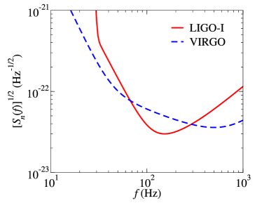
Figure 1: Square root of the noise spectral density $\sqrt{S_{n}(f)}$ versus frequency $f$, for LIGO-I [Eq. (28)], and VIRGO (from Tab. IV of Ref. DIS3 ).

$$\frac{S_{n}(f)}{{\rm Hz}^{-1}}=9.00\times 10^{-46}\,\left[\left(4.49\frac{f}{f_{0}}\right)^{-56}+0.16\left(\frac{f}{f_{0}}\right)^{-4.52}+0.52+0.32\left(\frac{f}{f_{0}}\right)^{2}\right]\,,$$ (28)

where $f_{0}=150$ Hz. The first term in the square brackets represents seismic noise, the second and third, thermal noise, and the fourth, photon shot noise.

Throughout this paper, we shall compute BBH waveforms in the quadrupole approximation (we shall compute the phase evolution of the GWs with the highest possible accuracy, but we shall omit all harmonics higher than the quadrupole, and we shall omit post–Newtonian corrections to the amplitude; this is a standard approach in the field, see, e.g., PN ). The signal received at the interferometer can then be written as KT300 ; Finnchernoff

$$h(t)=\frac{\Theta}{d_{\mathrm{L}}}M\eta(\pi Mf_{\mathrm{GW}})^{2/3}\cos\varphi_{\mathrm{GW}},$$ (29)

where $f$ and $\varphi_{\mathrm{GW}}$ are the instantaneous GW frequency and phase at the time $t$, $d_{\mathrm{L}}$ is the luminosity distance, $M$ and $\eta$ are respectively the BBH total mass $m_{1}+m_{2}$ and the dimensionless mass ratio $m_{1}m_{2}/M^{2}$, and where we have taken $G=c=1$. The coefficient $\Theta$ depends on the inclination of the BBH orbit with respect to the plane of the sky, and on the polarization and direction of propagation of the GWs with respect to the orientation of the interferometer. Finn and Chernoff Finnchernoff examine the distribution of $\Theta$, and show that $\Theta_{\mathrm{max}}=4$, while $\mathrm{rms}\,\Theta=8/5$. We shall use this last value when we compute optimal signal-to-noise ratios. The waveform given by Eq. (29), after dropping the factor $\Theta M\eta/d_{\mathrm{L}}$, is known as restricted waveform.

model	shorthand	evolution equation	section
	T$(n\mathrm{PN},m\mathrm{PN};\hat{\theta})$	energy-balance equation	Sec. III.1
	P$(n\mathrm{PN},m\mathrm{PN};\hat{\theta})$	energy-balance equation	Sec. III.2
	SPA$(n\mathrm{PN}\equiv m\mathrm{PN})$		Sec. VI.6
	HT$(n\mathrm{PN},m\mathrm{PN};\hat{\theta})$	Hamilton equations	Sec. IV.1
	HP$(n\mathrm{PN},m\mathrm{PN};\hat{\theta})$	Hamilton equations	Sec. IV.1
	L$(n\mathrm{PN},m\mathrm{PN})$	$\mathbf{F}=m\mathbf{a}$	Sec. IV.2
	ET$(n\mathrm{PN},m\mathrm{PN};\hat{\theta};\tilde{z}_{1},\tilde{z}_{2})$	eff. Hamilton equations	Sec. IV.3
	EP$(n\mathrm{PN},m\mathrm{PN};\hat{\theta};\tilde{z}_{1},\tilde{z}_{2})$	eff. Hamilton equations	Sec. IV.3

Table 1: Post–Newtonian models of two-body dynamics defined in this paper. The notation X$(n\mathrm{PN},m\mathrm{PN};\hat{\theta})$ denotes the model X, with terms up to order $n$PN for the conservative dynamics, and with terms up to order $m$PN for radiation-reaction effects; for $m\geq 3$ we also need to specify the arbitrary flux parameter $\hat{\theta}$ (see Sec. III.1); for $n\geq 3$, the effective-one-body models need also two additional parameters $\tilde{z}_{1}$ and $\tilde{z}_{2}$ (see Sec. IV.3).

III Adiabatic models

We turn, now, to a discussion of the currently available mathematical models for the inspiral of BBHs. Table 1 shows a list of the models that we shall consider in this paper, together with the shorthands that we shall use to denote them. We begin in this section with adiabatic models. BBH adiabatic models treat the orbital inspiral as a quasistationary sequence of circular orbits, indexed by the invariantly defined velocity

$$v=(M\dot{\varphi})^{1/3}=(\pi Mf_{\rm GW})^{1/3}.$$ (30)

The evolution of the inspiral (and in particular of the orbital phase $\varphi$) is completely determined by the energy-balance equation

$$\frac{d{\cal E}(v)}{dt}=-{\cal F}(v),$$ (31)

This equation relates the time derivative of the energy function ${\cal E}(v)$ (which is given in terms of the total relativistic energy ${\mathcal{E}}_{\mathrm{tot}}$ by $\mathcal{E}={\mathcal{E}}_{\mathrm{tot}}-m_{1}-m_{2}$, and which is conserved in absence of radiation reaction) to the gravitational flux (or luminosity) function ${\cal F}(v)$. Both functions are known for quasicircular orbits as a PN expansion in $v$. It is easily shown that Eq. (31) is equivalent to the system (see, e.g., Ref. DIS1 )

$$\frac{d\varphi_{\rm GW}}{dt}=\frac{2v^{3}}{M}\,,\quad\quad\frac{dv}{dt}=-\frac{{\cal F}(v)}{M\,d{\cal E}(v)/dv}.$$ (32)

In accord with the discussion around Eq. (29), we shall only consider the restricted waveform $h(t)=v^{2}\cos\varphi_{\rm GW}(t)$, where the GW phase $\varphi_{\rm GW}$ is twice the orbital phase $\varphi$.

III.1 Adiabatic PN expanded models

The equations of motion for two compact bodies at 2.5PN order were first derived in Refs. DD . The 3PN equations of motion have been obtained by two separate groups of researchers: Damour, Jaranowski and Schäfer DJS used the Arnowitt–Deser–Misner (ADM) canonical approach, while Blanchet, Faye and de Andrade DBF worked with the PN iteration of the Einstein equations in the harmonic gauge. Recently Damour and colleagues DJSd , working in the ADM formalism and applying dimensional regularization, determined uniquely the static parameter that enters the 3PN equations of motion DJS ; DBF and that was until then unknown. In this paper we shall adopt their value for the static parameter. Thus at present the energy function ${\cal E}$ is known up to 3PN order.

The gravitational flux emitted by compact binaries was first computed at 1PN order in Ref. 1PN . It was subsequently determined at 2PN order with a formalism based on multipolar and post–Minkowskian approximations, and, independently, with the direct integration of the relaxed Einstein equations 2PN . Nonlinear effects of tails at 2.5PN and 3.5PN orders were computed in Refs. 2.5PNand3.5PN . More recently, Blanchet and colleagues derived the gravitational-flux function for quasicircular orbits up to 3.5PN order BIJ ; BFIJ . However, at 3PN order BIJ ; BFIJ the gravitational-flux function depends on an arbitrary parameter $\hat{\theta}$ that could not be fixed in the regularization scheme used by these authors.

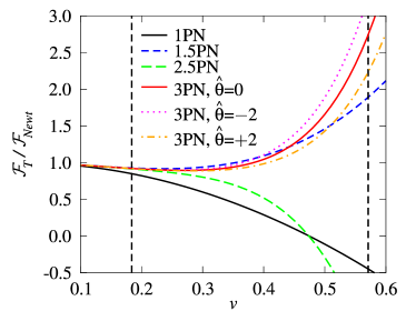
Figure 2: Normalized flux function ${\cal F}_{T_{N}}/{\cal F}_{\rm Newt}$ versus $v$, at different PN orders for equal-mass binaries, $\eta=0.25$. Note that the 1.5PN and 2PN flux, and the 3PN and 3.5PN flux, are so close that they cannot be distinguished in these plots. The two long-dashed vertical lines correspond to $v\simeq 0.18$ and $v\simeq 0.53$; they show the velocity range that corresponds to the LIGO frequency band $40\leq f_{\rm GW}\leq 240$ Hz for BBHs with total mass in the range $10\mbox{--}40M_{\odot}$.

PN energy and flux

Denoting by ${\cal E}_{T_{N}}$ and ${\cal F}_{T_{N}}$ the $N^{\rm th}$-order Taylor approximants (T-approximants) to the energy and the flux functions, we have

$${\cal E}_{T_{2N}}(v)\equiv{\cal E}_{\rm Newt}(v)\,\sum_{k=0}^{N}\,{\cal E}_{k}(\eta)\,v^{2k}\,,$$ (33)

$${\cal F}_{T_{N}}(v)\equiv{\cal F}_{\rm Newt}(v)\,\sum_{k=0}^{N}\,{\cal F}_{k}(\eta)\,v^{k}\,,$$ (34)

where “Newt” stands for Newtonian order, and the subscripts $2N$ and $N$ stand for post^2N–Newtonian and post^N–Newtonian order. The quantities in these equations are

$${\cal E}_{\rm Newt}(v)=-\frac{1}{2}\eta\,v^{2}\,,\quad\quad{\cal F}_{\rm Newt}(v)=\frac{32}{5}\eta^{2}\,v^{10}\,,$$ (35)

$${\cal E}_{0}(\eta)=1\,,\quad\quad{\cal E}_{1}(\eta)=-\frac{3}{4}-\frac{\eta}{12}\,,\quad\quad{\cal E}_{2}(\eta)=-\frac{27}{8}+\frac{19}{8}\eta-\frac{\eta^{2}}{24}\,,$$ (36)

$${\cal E}_{3}(\eta)=-\frac{675}{64}+\left(\frac{34445}{576}-\frac{205}{96}\pi^{2}\right)\eta-\frac{155}{96}\eta^{2}-\frac{35}{5184}\eta^{3}\,,$$ (37)

$${\cal F}_{0}(\eta)=1\,,\quad\quad{\cal F}_{1}(\eta)=0\,,\quad\quad{\cal F}_{2}(\eta)=-\frac{1247}{336}-\frac{35}{12}\eta\,,\quad\quad{\cal F}_{3}(\eta)=4\pi\,,\\$$ (38)

$${\cal F}_{4}(\eta)=-\frac{44711}{9072}+\frac{9271}{504}\eta+\frac{65}{18}\eta^{2}\,,\quad\quad{\cal F}_{5}(\eta)=-\left(\frac{8191}{672}+\frac{583}{24}\eta\right)\pi\,,$$ (39)

$${\cal F}_{6}(\eta) = \frac{6643739519}{69854400}+\frac{16}{3}\,\pi^{2}-\frac{1712}{105}\,\gamma_{E}-\frac{856}{105}\,\log(16v^{2})+$$ (40)

$$\left(-\frac{2913613}{272160}+\frac{41}{48}\,\pi^{2}-\frac{88}{3}\,\hat{\theta}\right)\eta-\frac{94403}{3024}\,\eta^{2}-\frac{775}{324}\,\eta^{3}\,,$$

$${\cal F}_{7}(\eta)=\left(-\frac{16285}{504}+\frac{214745}{1728}\eta+\frac{193385}{3024}\eta^{2}\right)\,\pi\,.$$ (41)

Here $\eta=m_{1}m_{2}/(m_{1}+m_{2})^{2}$, $\gamma_{E}$ is Euler’s gamma, and $\hat{\theta}$ is the arbitrary 3PN flux parameter BIJ ; BFIJ . From Tab. I of Ref. BFIJ we read that the extra number of GW cycles accumulated by the PN terms of a given order decreases (roughly) by an order of magnitude when we increase the PN order by one. Hence, we find it reasonable to expect that at 3PN order the parameter $\hat{\theta}$ should be of order unity, and we choose as typical values $\hat{\theta}=0,\pm 2$. (Note for v3 of this paper on gr-qc: Eqs. (39) and (41) are now revised as per Ref. errata ; the parameter $\hat{\theta}$ has been determined to be 1039/4620 thetapar .)

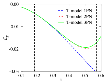
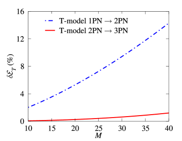
Figure 3: In the left panel, we plot the energy function ${\cal E}_{T_{N}}$ versus $v$, at different PN orders, for $\eta=0.25$. The two long-dashed vertical lines in the left figure correspond to $v\simeq 0.18$ and $v\simeq 0.53$; they show the velocity range that corresponds to the LIGO frequency band $40\leq f_{\rm GW}\leq 240$ Hz, for BBHs with total mass in the range $10\mbox{--}40M_{\odot}$. In the right panel, we plot the percentage difference $\delta{\cal E}_{T_{N}}=100\,|({\cal E}_{T_{N+1}}-{\cal E}_{T_{N}})/{\cal E}_{T_{N}}|$ versus the total mass $M$, for $N=1,2$, at the LIGO-I peak-sensitivity GW frequency, $f_{\mathrm{peak}}=153$ Hz [note: $v_{\mathrm{peak}}=(\pi Mf_{\mathrm{peak}})^{1/3}$].

In Fig. 2 we plot the normalized flux ${\mathcal{F}}_{T_{N}}/{\mathcal{F}}_{\rm Newt}$ as a function of $v$ at various PN orders for the equal mass case $\eta=0.25$. To convert $v$ to a GW frequency we can use

$$f_{\rm GW}\simeq 3.2\times 10^{4}\left(\frac{20M_{\odot}}{M}\right)v^{3}.$$ (42)

The two long-dashed vertical lines in Fig. 2 correspond to $v\simeq 0.18$ and $v\simeq 0.53$; they show the velocity range that corresponds to the LIGO frequency band $40\leq f_{\rm GW}\leq 240$ Hz for BBHs with total mass in the range $10\mbox{--}40M_{\odot}$. At the LIGO-I peak-sensitivity frequency, which is $153$ Hz according to our noise curve, and for a (10+10)$M_{\odot}$ BBH, we have $v\simeq 0.362$; and the percentage difference between subsequent PN orders is ${\rm Newt}\rightarrow 1{\rm PN}:-58\%$; $1{\rm PN}\rightarrow 1.5{\rm PN}:+142\%$; $1.5{\rm PN}\rightarrow 2{\rm PN}:-0.2\%$; $2{\rm PN}\rightarrow 2.5{\rm PN}:-34\%$; $2.5{\rm PN}\rightarrow 3{\rm PN}(\hat{\theta}=0):+43\%$; $3{\rm PN}\rightarrow 3.5{\rm PN}(\hat{\theta}=0):+0.04\%$. The percentage difference between the 3PN fluxes with $\hat{\theta}=\pm 2$ is $\sim 7\%$. It is interesting to notice that while there is a big difference between the 1PN and 1.5PN orders, and between the 2PN and 2.5PN orders, the 3PN and 3.5PN fluxes are rather close. Of course this observation is insufficient to conclude that the PN sequence is converging at 3.5PN order.

In the left panel of Fig. 3, we plot the T-approximants for the energy function versus $v$, at different PN orders, while in the right panel we plot (as a function of the total mass $M$, and at the LIGO-I peak-sensitivity GW frequency $f_{\mathrm{peak}}=153$ Hz) the percentage difference of the energy function between T-approximants to the energy function of successive PN orders. We note that the 1PN and 2PN energies are distant, but the 2PN and 3PN energies are quite close.

$M$	$f_{\rm GW}$(Hz) at MECO					$f_{\rm GW}$(Hz) at ISCO
	T (1PN)	T (2PN)	T (3PN)	P (2PN)	P (3PN)	H (1PN)	E (1PN)	E (2PN)	E (3PN)
$(5+5)M_{\odot}$	3376	886	832	572	866	183	446	473	570
$(10+10)M_{\odot}$	1688	442	416	286	433	92	223	236	285
$(15+15)M_{\odot}$	1125	295	277	191	289	61	149	158	190
$(20+20)M_{\odot}$	844	221	208	143	216	46	112	118	143

Table 2: Location of the MECO/ISCO. The first six columns show the GW frequency at the Maximum binding Energy for Circular Orbits (MECO), computed using the T- and P-approximants to the energy function; the remaining columns show the GW frequency at the Innermost Stable Circular Orbit (ISCO), computed using the H-approximant to the energy, and using the EOB improved Hamiltonian (90) with $\tilde{z}_{1}=\tilde{z}_{2}=0$. For the H-approximant the ISCO exists only at 1PN order.

Definition of the models

The evolution equations (32) for the adiabatic inspiral lose validity (the inspiral ceases to be adiabatic) a little before $v$ reaches $v_{\rm MECO}^{T_{N}}$, where MECO stands for Maximum–binding-Energy Circular Orbit LB ; DGG . This $v_{\rm MECO}^{T_{N}}$ is computed as the value of $v$ at which $d{\cal E}_{T_{N}}(v)/dv=0$. In building our adiabatic models we evolve Eqs. (32) right up to $v_{\mathrm{MECO}}$ and stop there. We shall refer to the frequency computed by setting $v=v_{\mathrm{MECO}}$ in Eq. (42) as the ending frequency for these waveforms, and in Tab. 2 we show this frequency for some BH masses. However, for certain binaries, the 1PN and 2.5PN flux functions can go to zero before $v=v_{\rm MECO}^{T_{N}}$ [see Fig. 2]. In those cases we choose as the ending frequency the value of $f=v^{3}/(\pi M)$ where ${\cal F}(v)$ becomes 10% of $\mathcal{F}_{\mathrm{Newt}}(v)$. [When using the 2.5PN flux, our choice of the ending frequency differs from the one used in Ref. DIS3 , where the authors stopped the evolution at the GW frequency corresponding to the Schwarzschild innermost stable circular orbit. For this reason there are some differences between our overlaps and theirs.]

We shall refer to the models discussed in this section as ${\rm T}(n{\rm PN},m{\rm PN})$, where $n$PN ($m$PN) denotes the maximum PN order of the terms included for the energy (the flux). We shall consider $(n{\rm PN},m{\rm PN})=(1,1.5),(2,2),(2,2.5)$ and $(3,3.5,\hat{\theta})$ [at 3PN order we need to indicate also a choice of the arbitrary flux parameter $\hat{\theta}$].

$N$	$\left<{\rm T}_{N},{\rm T}_{N+1}\right>$
	$(5+20)M_{\odot}$		$(10+10)M_{\odot}$				$(15+15)M_{\odot}$
0	0.432		0.553	(0.861,	19.1,	0.241)	0.617
1	0.528	[0.638]	0.550	(0.884,	22.0,	0.237)	0.645	[0.712]
2 ($\hat{\theta}=+2$)	0.482	[0.952]	0.547	(0.841,	18.5,	0.25)	0.563	[0.917]
2 ($\hat{\theta}=-2$)	0.457	[0.975]	0.509	(0.821,	18.7,	0.241)	0.524	[0.986]

Table 3: Test for the Cauchy convergence of the T-approximants. The values quoted are maxmax matches obtained by maximizing with respect to the extrinsic parameters, but not to the intrinsic parameters (i.e., the matches are computed for T waveforms with the same masses, but different PN orders). Here we define ${\rm T}_{0}={\rm T}(0,0)$, ${\rm T}_{1}={\rm T}(1,1.5)$, ${\rm T}_{2}={\rm T}(2,2.5)$, ${\rm T}_{3}={\rm T}(3,3.5,\hat{\theta})$. In the Newtonian case, ${\rm T}_{0}=(0,0)$, the MECO does not exist and we stop the integration of the balance equation at $v=1$. The values in brackets, “[…],” are obtained by setting ${\rm T}_{2}={\rm T}(2,2)$ instead of ${\rm T}(2,2.5)$; the values in parentheses, “(…),” are obtained by maximizing with respect to the extrinsic and intrinsic parameters, and they are shown together with the ${\rm T}_{N+1}$ parameters $M$ and $\eta$ where the maxima are achieved. In all cases the integration of the equations is started at a GW frequency of $20$ Hz.

Waveforms and matches

In Tab. 3, for three typical choices of BBH masses, we perform a convergence test using Cauchy’s criterion DIS1 , namely, the sequence ${\rm T}_{N}$ converges if and only if for each $k$, ${\langle{\rm T}_{N},{\rm T}_{N+k}\rangle}\rightarrow 1$ as $N\rightarrow\infty$. One requirement of this criterion is that ${\langle{\rm T}_{N},{\rm T}_{N+1}\rangle}\rightarrow 1$ as $N\rightarrow\infty$, and this is what we test in Tab. 3, setting $\mathrm{T}_{N}\equiv\mathrm{T}(N,N+0.5)$. The values quoted assume maximization on the extrinsic parameters but not on the intrinsic parameters. [For the case $(10+10)M_{\odot}$, we show in parentheses the maxmax matches obtained by maximizing with respect to the intrinsic and extrinsic parameters, together with the intrinsic parameters $M$ and $\eta$ of $\mathrm{T}_{N+1}$ where the maxima are attained.] These results suggest that the PN expansion is far from converging. However, the very low matches between $N=1$ and $N=2$, and between $N=2$ and $N=3$, are due to the fact that the 2.5PN flux goes to zero before the MECO can be reached. If we redefine $\mathrm{T}_{2}$ as $\mathrm{T}(2,2)$ instead of $\mathrm{T}(2,2.5)$, we obtain the higher values shown in brackets is Tab. 3.

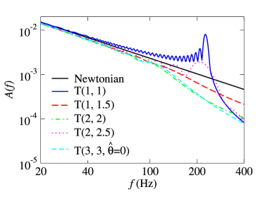
Figure 4: Frequency-domain amplitude versus frequency for the T-approximated (restricted) waveforms, at different PN orders, for a $(15+15)M_{\odot}$ BBH. The T$(3,3.5,\hat{\theta}=0)$ curve, not plotted, is almost identical to the T$(3,3,\hat{\theta}=0)$ curve.

In Fig. 4, we plot the frequency-domain amplitude of the T-approximated waveforms, at different PN orders, for a $(15+15)M_{\odot}$ BBH. The Newtonian amplitude, ${\cal A}_{\rm Newt}(f)=f^{-7/6}$, is also shown for comparison. In the $\mathrm{T}(1,1)$ and $\mathrm{T}(2,2.5)$ cases, the flux function goes to zero before $v=v_{\rm MECO}^{T_{N}}$; this means that the radiation-reaction effects become negligible during the last phase of evolution, so the binary is able to spend many cycles at those final frequencies, skewing the amplitude with respect to the Newtonian result. For $\mathrm{T}(2,2)$, $\mathrm{T}(3,3)$ and $\mathrm{T}(3,3.5)$, the evolution is stopped at $v=v_{\rm MECO}^{T_{N}}$, and, although $f_{\rm MECO}^{\rm GW}\simeq 270\mbox{--}300$ Hz (see Tab. 2) the amplitude starts to deviate from $f^{-7/6}$ around $100$ Hz. This is a consequence of the abrupt termination of the signal in the time domain.

The effect of the arbitrary parameter $\hat{\theta}$ on the T waveforms can be seen in Tab. IV.2 in the intersection between the rows and columns labeled T$(3,3.5,+2)$ and T$(3,3.5,-2)$. For three choices of BBH masses, this table shows the maxmax matches between the search models at the top of the columns and the target models at the left end of the rows, maximized over the mass parameters of the search models in the columns. These matches are rather high, suggesting that for the range of BBH masses we are concerned, the effect of changing $\hat{\theta}$ is just a remapping of the BBH mass parameters. Therefore, in the following we shall consider only the case of $\hat{\theta}=0$.

A quantitative measure of the difference between the $\mathrm{T}(2,2)$, $\mathrm{T}(2,2.5)$ and $\mathrm{T}(3,3.5)$ waveforms can be seen in Tab. IV.2 in the intersection between the rows and columns labeled T$(\ldots)$. For four choices of BBH masses, this table shows the maxmax matches between the search models in the columns and the target models in the rows, maximized over the search-model parameters $M$ and $\eta$; in the search, $\eta$ is restricted to its physical range $0<\eta\leq 1/4$, where $0$ corresponds to the test-mass limit, while $1/4$ is obtained in the equal-mass case. These matches can be interpreted as the fitting factors [see Eq. (20)] for the projection of the target models onto the search models. For the case $\mathrm{T}(2,2.5)$ the values are quite low: if the $\mathrm{T}(3,3.5)$ waveforms turned out to give the true physical signals and if we used the $\mathrm{T}(2,2.5)$ waveforms to detect them, we would lose $\sim 32\mbox{--}49\%$ of the events. The model $\mathrm{T}(2,2)$ would do match better, although it would still not be very faithful. Once more, the difference between $\mathrm{T}(2,2)$ and $\mathrm{T}(2,2.5)$ is due to the fact that the 2.5PN flux goes to zero before the BHs reach the MECO.

III.2 Adiabatic PN resummed methods: Padé approximants

The PN approximation outlined above can be used quite generally to compute the shape of the GWs emitted by BNSs or BBHs, but it cannot be trusted in the case of binaries with comparable masses in the range $M\simeq 10\mbox{--}40M_{\odot}$, because for these sources LIGO and VIRGO will detect the GWs emitted when the motion is strongly relativistic, and the convergence of the PN series is very slow. To cope with this problem, Damour, Iyer and Sathyaprakash DIS1 proposed a new class of models based on the systematic application of Padé resummation to the PN expansions of ${\cal E}(v)$ and ${\cal F}(v)$. This is a standard mathematical technique used to accelerate the convergence of poorly converging or even divergent power series.

If we know the function $g(v)$ only through its Taylor approximant $G_{N}(v)=g_{0}+g_{1}\,v+\cdots+g_{N}\,v^{N}\equiv T_{N}[g(v)]$, the central idea of Padé resummation BO is the replacement of the power series $G_{N}(v)$ by the sequence of rational functions

$$P_{K}^{M}[g(v)]=\frac{A_{M}(v)}{B_{K}(v)}\equiv\frac{\sum_{j=0}^{M}a_{j}\,v^{j}}{\sum_{j=0}^{K}b_{j}\,v^{j}}\,,$$ (43)

with $M+K=N$ and $T_{M+K}[P_{K}^{M}(v)]=G_{N}(v)$ (without loss of generality, we can set $b_{0}=1$). We expect that for $M,K\rightarrow+\infty$, $P_{K}^{M}[g(v)]$ will converge to $g(v)$ more rapidly than $T_{N}[g(v)]$ converges to $g(v)$ for $N\rightarrow+\infty$.

PN energy and flux

Damour, Iyer and Sathyaprakash DIS1 , and then Damour, Schäfer and Jaranowski EOB3PN , proposed the following Padé-approximated (P-approximated) ${\cal E}_{P_{N}}(v)$ and ${\cal F}_{P_{N}}(v)$ (for $N=2,3$):

$${\cal E}_{P_{N}} = \sqrt{1+2\eta\,\sqrt{1+e_{P_{N}}(v)}-1}-1\,,$$ (44)

$${\cal F}_{P_{N}} = \frac{32}{5}\eta^{2}\,v^{10}\,\frac{1}{1-v/v^{P_{N}}_{\rm pole}}\,f_{P_{N}}(v,\eta)\,,$$ (45)

where

$$e_{P_{2}}(v)=-v^{2}\,\frac{1+\frac{1}{3}\eta-\left(4-\frac{9}{4}\eta+\frac{1}{9}\eta^{2}\right)\,v^{2}}{1+\frac{1}{3}\eta-\left(3-\frac{35}{12}\eta\right)\,v^{2}}\,,$$ (46)

$$e_{P_{3}}(v)=-v^{2}\,\frac{1-\left(1+\frac{1}{3}\eta+w_{3}(\eta)\right)\,v^{2}-\left(3-\frac{35}{12}\eta-\left(1+\frac{1}{3}\eta\right)\,w_{3}(\eta)\right)\,v^{4}}{1-w_{3}(\eta)\,v^{2}}\,,$$ (47)

$$w_{3}=\frac{40}{36-35\eta}\,\left[\frac{27}{10}+\frac{1}{16}\left(\frac{41}{4}\pi^{2}-\frac{4309}{15}\right)\eta+\frac{103}{120}\eta^{2}-\frac{1}{270}\eta^{3}\right]\,,$$ (48)

$$f_{P_{2}}(v)=\left(1+\frac{c_{1}\,v}{1+\frac{c_{2}\,v}{1+\ldots}}\right)^{-1}\quad\text{(up to $c_{5}$)},$$ (49)

$$f_{P_{3}}(v)=\left(1-\frac{1712}{105}\,v^{6}\,\log\frac{v}{v_{\rm MECO}^{P_{2}}}\right)\,\left(1+\frac{c_{1}\,v}{1+\frac{c_{2}\,v}{1+\ldots}}\right)^{-1}\text{(up to $c_{7}$)}.$$ (50)

Here the dimensionless coefficients $c_{i}$ depend only on $\eta$. The $c_{k}$’s are explicit functions of the coefficients $f_{k}$ ($k=1,...5$),

$$c_{1}=-f_{1}\,,\quad\quad c_{2}=f_{1}-\frac{f_{2}}{f_{1}}\,,\quad\quad c_{3}=\frac{f_{1}\,f_{3}-f_{2}^{2}}{f_{1}\,(f_{1}^{2}-f_{2})}\,,$$ (51)

$$c_{4}=-\frac{f_{1}\,(f_{2}^{3}+f_{3}^{2}+f_{1}^{2}\,f_{4}-f_{2}\,(2\,f_{1}\,f_{3}+f_{4}))}{(f_{1}^{2}-f_{2})\,(f_{1}\,f_{3}-f_{2}^{2})}\,,$$ (52)

$$c_{5}=-\frac{(f_{1}^{2}-f_{2})\,(-f_{3}^{3}+2f_{2}\,f_{3}\,f_{4}-f_{1}\,f_{4}^{2}-f_{2}^{2}\,f_{5}+f_{1}\,f_{3}\,f_{5})}{(f_{1}\,f_{3}-f_{2}^{2})\,(f_{2}^{3}+f_{3}^{2}+f_{1}^{2}\,f_{4}-f_{2}\,(2\,f_{1}\,f_{3}+f_{4}))}\,,$$ (53)

where

$$f_{k}={\cal F}_{k}-\frac{{\cal F}_{k-1}}{v^{P_{2}}_{\rm pole}}\,.$$ (54)

Here ${\cal F}_{k}$ is given by Eqs. (38)–(41) [for $k=6$ and $k=7$, the term $-856/105\log 16v^{2}$ should be replaced by $-856/105\log 16(v^{P_{2}}_{\rm MECO})^{2}$]. The coefficients $c_{7}$ and $c_{8}$ are straightforward to compute, but we do not show them because they involve rather long expressions. The quantity $v^{P_{2}}_{\rm MECO}$ is the MECO of the energy function $e_{P_{2}}$ [defined by $de_{P_{2}}(v)/dv=0$].

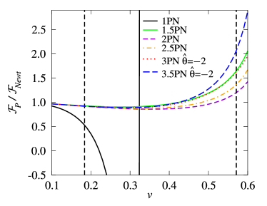
Figure 5: Normalized flux function ${\cal F}_{P_{N}}/{\cal F}_{\rm Newt}$ versus $v$, at different PN orders. The two long-dashed vertical lines give $v\simeq 0.18$ and $v\simeq 0.53$; they show the velocity range that corresponds to the LIGO frequency band $40\leq f_{\rm GW}\leq 240$ Hz for BBHs with total mass in the range $10\mbox{--}40M_{\odot}$. Compare with Fig. 2.

The quantity $v^{P_{2}}_{\rm pole}$, given by

$$v^{P_{2}}_{\rm pole}=\frac{1}{\sqrt{3}}\,\sqrt{\frac{1+\frac{1}{3}\eta}{1-\frac{35}{36}\eta}}\,,$$ (55)

is the pole of $e_{P_{2}}$, which plays an important role in the scheme proposed by Damour, Iyer and Sathyaprakash DIS1 . It is used to augment the Padé resummation of the PN expanded energy and flux with information taken from the test-mass case, where the flux (known analytically up to 5.5PN order) has a pole at the light ring. Under the hypothesis of structural stability DIS1 , the flux should have a pole at the light ring also in the comparable-mass case. In the test-mass limit, the light ring corresponds to the pole of the energy, so the analytic structure of the flux is modified in the comparable-mass case to include $v^{P_{2}}_{\rm pole}(\eta)$. At 3PN order, where the energy has no pole, we choose (somewhat arbitrarily) to keep using the value $v^{P_{2}}_{\rm pole}(\eta)$; the resulting 3PN approximation to the test-mass flux is still very good.

In Fig. 5, we plot the P-approximants for the flux function $\mathcal{F}_{P_{N}}$(v), at different PN orders. Note that at 1PN order the P-approximant has a pole. At the LIGO-I peak-sensitivity frequency, $153$ Hz, for a (10+10)$M_{\odot}$ BBH, the value of $v$ is $\simeq 0.362$, and the percentage difference in $\mathcal{F}_{P_{N}}(0.362)$, between successive PN orders is $1.5{\rm PN}\rightarrow 2{\rm PN}:-8\%$; $2{\rm PN}\rightarrow 2.5{\rm PN}:+2.2\%$; $2.5{\rm PN}\rightarrow 3{\rm PN}\,(\hat{\theta}=-2):+3.6\%$; $3{\rm PN}\rightarrow 3.5{\rm PN}\,(\hat{\theta}=-2):+0.58\%$. So the percentage difference decreases as we increase the PN order. While in the test-mass limit it is known that the P-approximants converge quite well to the known exact flux function (see Fig. 3 of Ref. DIS1 ), in the equal-mass case we cannot be sure that the same is happening, because the exact flux function is unknown. (If we assume that the equal-mass flux function is a smooth deformation of the test-mass flux function, with $\eta$ the deformation parameter, then we could expect that the P-approximants are converging.)

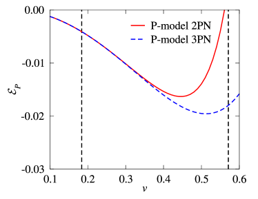
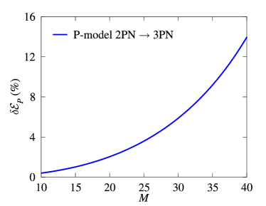
Figure 6: In the left panel, we plot the energy function ${\cal E}_{P_{N}}$ versus $v$, at different PN orders. In the right panel, we plot the percentage difference between 2PN and 3PN P-approximants, $\delta{\cal E}_{P}(v_{\mathrm{peak}})=100\,|[{\cal E}_{P_{3}}(v_{\mathrm{peak}})-{\cal E}_{P_{2}}(v_{\mathrm{peak}})]/{\cal E}_{P_{2}}(v_{\mathrm{peak}})|$ versus the total mass $M$, again evaluated at the LIGO-I peak-sensitivity GW frequency $f_{\mathrm{peak}}=153$ Hz [note: $v_{\mathrm{peak}}=(\pi Mf_{\mathrm{peak}})^{1/3}$].

In the left panel of Fig. 6, we plot the P-approximants to the energy function as a function of $v$, at 2PN and 3PN orders; in the right panel, we plot the percentage difference between 2PN and 3PN P-approximants to the energy function, as a function of the total mass $M$, evaluated at the LIGO-I peak-sensitivity GW frequency $f_{\mathrm{peak}}=153$ Hz.

$N$	$\left<P_{N},P_{N+1}\right>$
	$(20+5)M_{\odot}$	$(10+10)M_{\odot}$				$(15+15)M_{\odot}$
2 ($\hat{\theta}=+2$)	0.902	0.915	(0.973,	20.5,	0.242)	0.868
2 ($\hat{\theta}=-2$)	0.931	0.955	(0.982,	20.7,	0.236)	0.923

Table 4: Test for the Cauchy convergence of the P-approximants. The values quoted are maxmax matches obtained by maximizing with respect to the extrinsic parameters, but not to the intrinsic parameters (i.e., the matches are computed for P waveforms with the same masses, but different PN orders). Here we define $\mathrm{P}_{2}=\mathrm{P}(2,2.5)$, $\mathrm{P}_{3}=\mathrm{P}(3,3.5)$. The values in parentheses are the maxmax matches obtained by maximizing with respect to the extrinsic and intrinsic parameters, shown together with the $\mathrm{P}_{N+1}$ parameters $M$ and $\eta$ where the maxima are attained. In all cases the integration of the equations is started at a GW frequency of $20$ Hz.

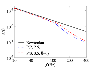
Figure 7: Frequency-domain amplitude versus frequency for the P-approximated (restricted) waveform, at different PN orders, for a $(15+15)M_{\odot}$ BBH.

Definition of the models

When computing the waveforms for P-approximant adiabatic models, the integration of the Eqs. (32) is stopped at $v=v_{\rm MECO}^{P_{N}}$, which is the solution of the equation $d{\cal E}_{P_{N}}(v)/dv=0$. The corresponding GW frequency will be the ending frequency for these waveforms, and in Tab. 2 we show this frequency for typical BBH masses. Henceforth, we shall refer to the P-approximant models as ${\rm P}(n{\rm PN},m{\rm PN})$, and we shall consider $(n{\rm PN},m{\rm PN})=(2,2.5),(3,3.5,\hat{\theta})$. [Recall that $n$PN and $m$PN are the maximum post–Newtonian order of the terms included, respectively, in the energy and flux functions $\mathcal{E}(v)$ and $\mathcal{F}(v)$; at 3PN order we need to indicate also a choice of the arbitrary flux parameter $\hat{\theta}$.]

Waveforms and matches

In Tab. 4, for three typical choices of BBH masses, we perform a convergence test using Cauchy’s criterion DIS1 . The values are quite high, especially if compared to the same test for the T-approximants when the 2.5PN flux is used, see Tab. 3. However, as we already remarked, we do not have a way of testing whether they are converging to the true limit. In Fig. 7, we plot the frequency-domain amplitude of the P-approximated (restricted) waveform, at different PN orders, for a $(15+15)M_{\odot}$ BBH. The Newtonian amplitude, ${\cal A}_{\rm Newt}(f)=f^{-7/6}$, is also shown for comparison. At 2.5PN and 3.5PN orders, the evolution is stopped at $v=v_{\rm MECO}^{P_{N}}$; although $f_{\rm MECO}^{\rm GW}\simeq 190-290$ Hz (see Tab. 2), the amplitude starts to deviate from $f^{-7/6}$ around $100$ Hz, well inside the LIGO frequency band. Again, this is a consequence of the abrupt termination of the signal in the time domain.

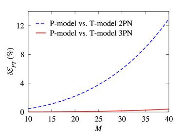
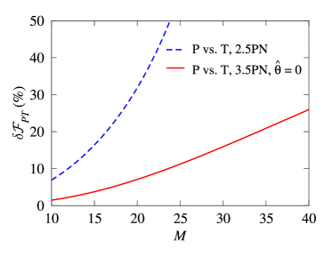
Figure 8: In the left panel, we plot the percentage difference $\delta{\cal E}_{PT}(v_{\mathrm{peak}})=100\,|[{\cal E}_{P_{N}}(v_{\mathrm{peak}})-{\cal E}_{T_{N}}(v_{\mathrm{peak}})]/{\cal E}_{P_{N}}(v_{\mathrm{peak}})|$ versus the total mass $M$, for $N=2,3$, at the LIGO-I peak-sensitivity GW frequency $f_{\mathrm{peak}}=153$ Hz [note: $v_{\mathrm{peak}}=(\pi Mf_{\mathrm{peak}})^{1/3}$]. In the right panel, we plot the percentage difference between 2PN and 3PN P-approximants, $\delta{\cal F}_{P}(v_{\mathrm{peak}})=100\,|[{\cal F}_{P_{3}}(v_{\mathrm{peak}})-{\cal F}_{P_{2}}(v_{\mathrm{peak}})]/{\cal F}_{P_{2}}(v_{\mathrm{peak}})|$ versus the total mass $M$, again evaluated at the LIGO-I peak-sensitivity GW frequency $f_{\mathrm{peak}}=153$ Hz.

A quantitative measure of the difference between the $\mathrm{P}(2,2.5)$ and $\mathrm{P}(3,3.5)$ waveforms can be seen in Tab. IV.2 in the intersection between the rows and columns labeled P$(\ldots)$. For three choices of BBH masses, this table shows the maxmax matches between the search models in the columns and the target models in the rows, maximized over the search-model parameters $M$ and $\eta$, with the restriction $0<\eta\leq 1/4$. These matches are quite high, but the models are not very faithful to each other. The same table shows also the maximized matches (i.e., fitting factors) between T and P models. These matches are low between $\mathrm{T}(2,2.5)$ and $\mathrm{P}(2,2.5)$ (and viceversa), between $\mathrm{T}(2,2.5)$ and $\mathrm{P}(3,3.5)$ (and viceversa), but they are high between $\mathrm{T}(2,2)$, $\mathrm{T}(3,3.5)$ and 3PN P-approximants (although the estimation of mass parameters is imprecise). Why this happens can be understood from Fig. 8 by noticing that at 3PN order the percentage difference between the T-approximated and P-approximated binding energies is rather small ($\leq 0.5\%$), and that the percentage difference between the T-approximated and P-approximated fluxes at 3PN order (although still $\sim 10\%$) is much smaller than at 2PN order.

IV Nonadiabatic models

By contrast with the models discussed in Sec. III, in nonadiabatic models we solve equations of motions that involve (almost) all the degrees of freedom of the BBH systems. Once again, all waveforms are computed in the restricted approximation of Eq. (29), taking the GW phase $\varphi_{\mathrm{GW}}$ as twice the orbital phase $\varphi$.

IV.1 Nonadiabatic PN expanded methods: Hamiltonian formalism

Working in the ADM gauge, Damour, Jaranowski and G. Schäfer have derived a PN expanded Hamiltonian for the general-relativistic two-body dynamics DJS ; DJSd ; EOB3PN :

$$\widehat{H}({\mathbf{q}},{\mathbf{p}})=\widehat{H}_{\rm Newt}({\mathbf{q}},{\mathbf{p}})+\widehat{H}_{\rm 1PN}({\mathbf{q}},{\mathbf{p}})+\widehat{H}_{\rm 2PN}({\mathbf{q}},{\mathbf{p}})+\widehat{H}_{\rm 3PN}({\mathbf{q}},{\mathbf{p}})\,,$$ (56)

where

$$\widehat{H}_{\rm Newt}\left({\bf q},{\bf p}\right) = \frac{{\bf p}^{2}}{2}-\frac{1}{q}\,,$$ (57)

$$\widehat{H}_{\rm 1PN}\left({\bf q},{\bf p}\right) = \frac{1}{8}(3\eta-1)({\bf p}^{2})^{2}-\frac{1}{2}\left[(3+\eta){\bf p}^{2}+\eta({\bf n}\cdot{\bf p})^{2}\right]\frac{1}{q}+\frac{1}{2q^{2}}\,,$$ (58)

$$\widehat{H}_{\rm 2PN}\left({\bf q},{\bf p}\right) = \frac{1}{16}\left(1-5\eta+5\eta^{2}\right)({\bf p}^{2})^{3}+\frac{1}{8}\left[\left(5-20\eta-3\eta^{2}\right)({\bf p}^{2})^{2}-2\eta^{2}({\bf n}\cdot{\bf p})^{2}{\bf p}^{2}-3\eta^{2}({\bf n}\cdot{\bf p})^{4}\right]\frac{1}{q}$$ (59)

$$+\frac{1}{2}\left[(5+8\eta){\bf p}^{2}+3\eta({\bf n}\cdot{\bf p})^{2}\right]\frac{1}{q^{2}}-\frac{1}{4}(1+3\eta)\frac{1}{q^{3}}\,,$$

$$\widehat{H}_{\rm 3PN}\left({\bf q},{\bf p}\right) = \frac{1}{128}\left(-5+35\eta-70\eta^{2}+35\eta^{3}\right)({\bf p}^{2})^{4}$$ (60)

$$+\frac{1}{16}\left[\left(-7+42\eta-53\eta^{2}-5\eta^{3}\right)({\bf p}^{2})^{3}+(2-3\eta)\eta^{2}({\bf n}\cdot{\bf p})^{2}({\bf p}^{2})^{2}+3(1-\eta)\eta^{2}({\bf n}\cdot{\bf p})^{4}{\bf p}^{2}-5\eta^{3}({\bf n}\cdot{\bf p})^{6}\right]\frac{1}{q}$$

$$+\left[\frac{1}{16}\left(-27+136\eta+109\eta^{2}\right)({\bf p}^{2})^{2}+\frac{1}{16}(17+30\eta)\eta({\bf n}\cdot{\bf p})^{2}{\bf p}^{2}+\frac{1}{12}(5+43\eta)\eta({\bf n}\cdot{\bf p})^{4}\right]\frac{1}{q^{2}}$$

$$+\left\{\left[-\frac{25}{8}+\left(\frac{1}{64}\pi^{2}-\frac{335}{48}\right)\eta-\frac{23}{8}\eta^{2}\right]{\bf p}^{2}+\left(-\frac{85}{16}-\frac{3}{64}\pi^{2}-\frac{7}{4}\eta\right)\eta({\bf n}\cdot{\bf p})^{2}\right\}\frac{1}{q^{3}}$$

$$+\left[\frac{1}{8}+\left(\frac{109}{12}-\frac{21}{32}\pi^{2}\right)\eta\right]\frac{1}{q^{4}}.$$

Here the reduced Non–Relativistic Hamiltonian in the center-of-mass frame, $\widehat{H}\equiv H^{\rm NR}/\mu$, is written as a function of the reduced canonical variables ${\bf p}\equiv{\bf p_{1}}/\mu=-{\bf p_{2}}/\mu$, and ${\bf q}\equiv({\bf x}_{1}-{\bf x}_{2})/M$, where ${\bf x_{1}}$ and ${\bf x_{2}}$ are the positions of the BH centers of mass in quasi–Cartesian ADM coordinates (see Refs. DJS ; DJSd ; EOB3PN ); the scalars $q$ and $p$ are the (coordinate) lengths of the two vectors; and the vector ${\bf n}$ is just ${\bf q}/q$.

Equations of motion

We now restrict the motion to a plane, and we introduce radiation-reaction (RR) effects as in Ref. BD2 . The equations of motion then read (using polar coordinates $r$ and $\varphi$ obtained from the $\mathbf{q}$ with the usual Cartesian-to-polar transformation)

$$\frac{dr}{d\widehat{t}}=\frac{\partial\widehat{H}}{\partial p_{r}}(r,p_{r},p_{\varphi})\,,\quad\frac{d\varphi}{d\widehat{t}}\equiv\widehat{\omega}=\frac{\partial\widehat{H}}{\partial p_{\varphi}}(r,p_{r},p_{\varphi})\,,$$ (61)

$$\frac{dp_{r}}{d\widehat{t}}=-\frac{\partial\widehat{H}}{\partial r}(r,p_{r},p_{\varphi})+\widehat{F}^{r}(r,p_{r},p_{\varphi})\,,\quad\frac{dp_{\varphi}}{d\widehat{t}}=\widehat{F}^{\varphi}[\widehat{\omega}(r,p_{r},p_{\varphi})]\,,$$ (62)

where $\widehat{t}=t/M$, $\widehat{\omega}=\omega M$; and where $\widehat{F}^{\varphi}\equiv{F}^{\varphi}/\mu$ and $\widehat{F}^{r}\equiv{F}^{r}/\mu$ are the reduced angular and radial components of the RR force. Assuming ${F}^{r}\ll{F}^{\varphi}$ BD2 , averaging over an orbit, and using the balance equation (31), we can express the angular component of the radiation-reaction force in terms of the GW flux at infinity BD2 . More explicitly, if we use the P-approximated flux, we have

$$\widehat{F}^{\varphi}\equiv{F}_{P_{N}}[v_{\omega}]=-\frac{1}{\eta\,v_{\omega}^{3}}\,{\cal F}_{P_{N}}[v_{\omega}]=-\frac{32}{5}\,\eta\,v_{\omega}^{7}\,\frac{f_{P_{N}}(v_{\omega};\eta)}{1-v_{\omega}/v_{\rm pole}^{P_{2}}(\eta)}\,,$$ (63)

while if we use the T-approximated flux we have

$$\widehat{F}^{\varphi}\equiv{F}_{T_{N}}[v_{\omega}]=-\frac{1}{\eta\,v_{\omega}^{3}}\,{\cal F}_{T_{N}}[v_{\omega}],$$ (64)

where $v_{\omega}\equiv\widehat{\omega}^{1/3}\equiv(d\varphi/d\widehat{t})^{1/3}$. This $v_{\omega}$ is used in Eq. (29) to compute the restricted waveform. Note that at each PN order, say $n$PN, we define our Hamiltonian model by evolving the Eqs. (61) and (62) without truncating the partial derivatives at the $n$PN order (differentiation with respect to the canonical variables can introduce terms of order higher than $n$PN). Because of this choice, and because of the approximation used to incorporate radiation-reaction effects, these nonadiabatic models are not, strictly speaking, purely post–Newtonian.

Innermost stable circular orbit

Circular orbits are defined by setting $r=\mathrm{constant}$ while neglecting radiation-reaction effects. In our PN Hamiltonian models, this implies $\partial\widehat{H}/\partial p_{r}=0$ through Eq. (61); because at all PN orders the Hamiltonian $\widehat{H}$ [Eqs. (56)–(60)] is quadratic in $p_{r}$, this condition is satisfied for $p_{r}=0$; in turn, this implies also $\partial\widehat{H}/\partial r=0$ [through Eq. (62)], which can be solved for $p_{\varphi}$. The orbital frequency is then given by $\hat{\omega}=\partial\widehat{H}/\partial p_{\varphi}$.

The stability of circular orbits under radial perturbations depends on the second derivative of the Hamiltonian:

$$\frac{\partial^{2}\widehat{H}}{\partial r^{2}}>0\Leftrightarrow\mathrm{stable\,\,orbit}\,;\quad\quad\frac{\partial^{2}\widehat{H}}{\partial r^{2}}<0\Leftrightarrow\mathrm{unstable\,\,orbit}\,.$$ (65)

For a test particle in Schwarzschild geometry (the $\eta\rightarrow 0$ of a BBH), an Innermost Stable Circular Orbit (ISCO) always exists, and it is defined by

$${\rm ISCO\,\,(Schwarzschild)}:\quad{\frac{\partial\widehat{H}^{\rm Schw}}{\partial r}}_{|_{p_{r}=0}}={\frac{\partial^{2}\widehat{H}^{\rm Schw}}{\partial r^{2}}}_{|_{p_{r}=0}}=0,$$ (66)

where $\widehat{H}^{\rm Schw}(r,p_{r},p_{\varphi})$ is the (reduced) nonrelativistic test-particle Hamiltonian in the Schwarzschild geometry. Similarly, if such an ISCO exists for the (reduced) nonrelativistic PN Hamiltonian $\widehat{H}$ [Eq. (56)], it is defined by

$${\rm ISCO\,\,(Hamiltonian)}:\quad{\frac{\partial\widehat{H}}{\partial r}}_{|_{p_{r}=0}}={\frac{\partial^{2}\widehat{H}}{\partial r^{2}}}_{|_{p_{r}=0}}=0.$$ (67)

Any inspiral built as an adiabatic sequence of quasicircular orbits cannot be extended to orbital separations smaller than the ISCO. In our model, we integrate the Hamiltonian equations (61) and (62) including terms up to a given PN order, without re-truncating the equations to exclude terms of higher order that have been generated by differentiation with respect to the canonical variables. Consistently, the value of the ISCO that is relevant to our model should be derived by solving Eq. (67) without any further PN truncation.

How is the ISCO related to the Maximum binding Energy for Circular Orbit (MECO), used above for nonadiabatic models such as T? The PN expanded energy for circular orbits ${\cal E}_{T_{n}}(\widehat{\omega})$ at order $n$PN can be recovered by solving the equations

$$\frac{\partial\widehat{H}(r,p_{r}=0,p_{\varphi})}{\partial r}=0,\quad\quad\frac{\partial\widehat{H}(r,p_{r}=0,p_{\varphi})}{\partial p_{\varphi}}=\hat{\omega},$$ (68)

for $r$ and $p_{\varphi}$ as functions of $\hat{\omega}$, and by using the solutions to define

$$\widehat{H}(\hat{\omega})\equiv\widehat{H}[r(\hat{\omega}),p_{r}=0,p_{\varphi}(\hat{\omega})].$$ (69)

Then $\widehat{H}(\hat{\omega}\equiv v^{3})=\mathcal{E}_{T_{n}}(v)$ as given by Eq. (33), if and only if in this procedure we are careful to eliminate all terms of order higher than $n$PN (see, e.g., Ref. LB ).

In the context of nonadiabatic models, the MECO is then defined by

$${\rm MECO}:\quad\quad\frac{d\widehat{H}}{d\widehat{\omega}}=0;$$ (70)

and it also characterizes the end of adiabatic sequences of circular orbits. Computing the variation of Eq. (69) between nearby circular orbits, and setting $p_{r}=0$, $dp_{r}=0$, we get

$$d\widehat{\omega}=\frac{\partial^{2}\widehat{H}}{\partial r\partial p_{\varphi}}\,dr+\frac{\partial^{2}\widehat{H}}{\partial p_{\varphi}^{2}}\,dp_{\varphi}\,,\quad\quad\frac{\partial^{2}\widehat{H}}{\partial r^{2}}\,dr+\frac{\partial^{2}\widehat{H}}{\partial r\partial p_{\varphi}}\,dp_{\varphi}=0\,;$$ (71)

and combining these two equations we get

$$\frac{dp_{\varphi}}{d\widehat{\omega}}=-\frac{\partial^{2}\widehat{H}}{\partial r^{2}}\,\left[\left(\frac{\partial^{2}\widehat{H}}{\partial r\partial p_{\varphi}}\right)^{2}-\frac{\partial^{2}\widehat{H}}{\partial p_{\varphi}^{2}}\,\frac{\partial^{2}\widehat{H}}{\partial r^{2}}\right]^{-1}\,.$$ (72)

So finally we can write

$$\frac{d\widehat{H}}{d\widehat{\omega}}=\frac{\partial\widehat{H}}{\partial p_{\varphi}}\,\frac{dp_{\varphi}}{d\widehat{\omega}}=-\frac{\partial^{2}\widehat{H}}{\partial r^{2}}\,\frac{\partial\widehat{H}}{\partial p_{\varphi}}\,\left[\left(\frac{\partial^{2}\widehat{H}}{\partial r\partial p_{\varphi}}\right)^{2}-\frac{\partial^{2}\widehat{H}}{\partial p_{\varphi}^{2}}\,\frac{\partial^{2}\widehat{H}}{\partial r^{2}}\right]^{-1}\,.$$ (73)

Not surprisingly, Eqs. (73) and (69) together are formally equivalent to the definition of the ISCO, Eq. (67) [note that the second and third terms on the right-hand side of Eq. (73) are never zero.] Therefore, if we knew the Hamiltonian $\widehat{H}$ exactly, we would find that the MECO defined by Eq. (70), is numerically the same as the ISCO defined by Eq. (67). Unfortunately, we are working only up to a finite PN order (say $n$PN); thus, to recover the MECO as given by Eq. (33), all three terms on the right-hand side of Eq. (73) must be written in terms of $\widehat{\omega}$, truncated at $n$PN order, then combined and truncated again at $n$PN order. This value of the MECO, however, will no longer be the same as the ISCO obtained by solving Eq. (67) exactly without truncation.

If the PN expansion was converging rapidly, then the difference between the ISCO and the MECO would be mild; but for the range of BH masses that we consider the PN convergence is bad, and the discrepancy is rather important. The ISCO is present only at 1PN order, with $r_{\mathrm{ISCO}}=9.907$ and $\widehat{\omega}_{\rm ISCO}=0.02833$. The corresponding GW frequencies are given in Tab. 2 for a few BBHs with equal masses. At 3PN order we find the formal solution $r^{\rm ISCO}=1.033$ and $p_{\varphi}^{\rm ISCO}=0.355$, but since we do not trust the PN expanded Hamiltonian when the radial coordinate gets so small, we conclude that there is no ISCO at 3PN order.

$N$	$\left<{\rm HT}_{N},{\rm HT}_{N+1}\right>$						$\left<{\rm HP}_{N},{\rm HP}_{N+1}\right>$
	$(5+20)M_{\odot}$	$(10+10)M_{\odot}$				$(15+15)M_{\odot}$	$(5+20)M_{\odot}$	$(10+10)M_{\odot}$				$(15+15)M_{\odot}$
0	0.118	0.191	(0.553,	13.7,	0.243)	0.206	0.253	0.431	(0.586,	16.7,	0.242)	0.316
1	0.102	0.174	(0.643,	61.0,	0.240)	0.170	0.096	0.161	(0.623,	17.4,	0.239)	0.151
2 ($\hat{\theta}=+2$)	0.292	0.476	(0.656,	18.6,	0.241)	0.377	0.266	0.369	(0.618,	17.6,	0.240)	0.325
2 ($\hat{\theta}=-2$)	0.287	0.431	(0.671,	19.0,	0.241)	0.377	0.252	0.354	(0.622,	17.4,	0.239)	0.312

Table 5: Test for the Cauchy convergence of the HT- and HP-approximants. The values quoted are maxmax matches obtained by maximizing with respect to the extrinsic parameters, but not to the intrinsic parameters (i.e., the matches are computed for H waveforms with the same masses, but different PN orders). Here we define $\mathrm{HT}_{0}=\mathrm{HT}(0,0)$, $\mathrm{HT}_{1}=\mathrm{HT}(1,1.5)$, $\mathrm{HT}_{2}=\mathrm{HT}(2,2)$ [because the 2.5PN flux goes to zero before the MECO is reached, so we use the 2PN flux], $\mathrm{HT}_{3}=\mathrm{HT}(3,3.5,\hat{\theta})$; we also define $\mathrm{HP}_{0}=\mathrm{HP}(0,0)$, $\mathrm{HP}_{1}=\mathrm{HP}(1,1.5)$, $\mathrm{HP}_{2}=\mathrm{HP}(2,2.5)$, and $\mathrm{HP}_{3}=\mathrm{HP}(3,3.5,\hat{\theta})$. The values in parentheses are the maxmax matches obtained by maximizing with respect to the extrinsic and intrinsic parameters, shown together with the $\mathrm{H}_{N+1}$ parameters $M$ and $\eta$ where the maxima are attained. In all cases the integration of the equations is started at a GW frequency of $20$ Hz.

Definition of the models

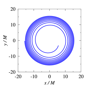
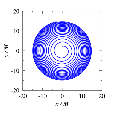
Figure 9: Inspiraling orbits in $(x,y)$-plane when $\eta=0.25$ for HT$(1,1.5)$ (in the left panel) and HT$(3,3.5,0)$ (in the right panel). For a $(15+15)M_{\odot}$ BBH the evolution starts at $f_{\rm GW}=34$ Hz and ends at $f_{\rm GW}=97$ Hz for HT$(1,1.5)$ panel and at $f_{\rm GW}=447$ Hz for HT$(3,3.5,0)$. The dynamical evolution is rather different because at 1PN order there is an ISCO ($r_{\rm ISCO}\simeq 9.9M$), while at 3PN order it does not exist.

In order to build a quasicircular orbit with initial GW frequency $f_{0}$, our initial conditions $(r_{\rm init},p_{r\,\rm init},p_{\varphi\,\rm init})$ are set by imposing $\dot{\varphi}_{\rm init}=\pi f_{0}$, $\dot{p}_{r\,\rm init}=0$ and $dr_{\rm init}/d\hat{t}=-{\cal F}/(\eta d\hat{H}/dr)_{\rm circ}$, as in Ref. DIS2 . The initial orbital phase $\varphi_{\rm init}$ remains a free parameter. For these models, the criterion used to stop the integration of Eqs. (61), (62) is rather arbitrary. We decided to push the integration of the dynamical equations up to the time when we begin to observe unphysical effects due to the failure of the PN expansion, or when the assumptions that underlie Eqs. (62) [such as $\widehat{F}^{r}\ll\widehat{F}^{\varphi}$], cease to be valid. When the 2.5PN flux is used, we stop the integration when ${\cal F}_{T_{N}}$ equals 10% of ${\cal F}_{\rm Newt}$, and we define the ending frequency for these waveforms as the instantaneous GW frequency at that time. To be consistent with the assumption of quasicircular motion, we require also that the radial velocity be always much smaller than the orbital velocity, and we stop the integration when $|\dot{r}|>0.3(r\dot{\varphi})$, if this occurs before ${\cal F}_{T_{N}}$ equals 10% of ${\cal F}_{\rm Newt}$. In some cases, during the last stages of inspiral $\widehat{\omega}$ reaches a maximum and then drops quickly to zero [see discussion in Sec. V]. When this happens, we stop the evolution at $\dot{\widehat{\omega}}=0$.

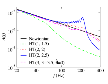
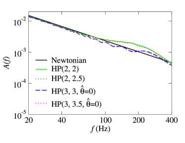
Figure 10: Frequency-domain amplitude versus frequency for the HT and HP (restricted) waveforms, at different PN orders, for a $(15+15)M_{\odot}$ BBH. The HT$(3,3.5,\hat{\theta}=0)$ curve, not plotted, is almost identical to the HT$(3,3,\hat{\theta}=0)$ curve.

We shall refer to these models as ${\rm HT}(n{\rm PN},m{\rm PN})$ (when the T-approximant is used for the flux) or ${\rm HP}(n{\rm PN},m{\rm PN})$ (when the P-approximant is used for the flux), where $n$PN ($m$PN) denotes the maximum PN order of the terms included in the Hamiltonian (the flux). We shall consider $(n\mathrm{PN},m\mathrm{PN})=(1,1.5),(2,2),(2,2.5)$, and $(3,3.5,\hat{\theta})$ [at 3PN order we need to indicate also a choice of the arbitrary flux parameter $\hat{\theta}$].

Waveforms and matches

In Tab. 5, for three typical choices of BBH masses, we perform a convergence test using Cauchy’s criterion DIS1 . The values are very low. For $N=0$ and $N=1$, the low values are explained by the fact that at 1PN order there is an ISCO [see the discussion below Eq. (73)], while at Newtonian and 2PN, 3PN order there is not. Because of the ISCO, the stopping criterion [$|\dot{r}|>0.3(r\dot{\varphi})$ or $\dot{\widehat{\omega}}=0$] is satisfied at a much lower frequency, hence at 1PN order the evolution ends much earlier than in the Newtonian and 2PN order cases. In Fig. 9, we show the inspiraling orbits in the $(x,y)$ plane for equal-mass BBHs, computed using the HT$(1,1.5)$ model (in the left panel) and the HT$(3,3.5,0)$ model (in the right panel). For $N=2$, the low values are due mainly to differences in the conservative dynamics, that is, to differences between the 2PN and 3PN Hamiltonians. Indeed, for a $(10+10)M_{\odot}$ BBH we find $\left<{\rm HT}(2,2),{\rm HT}(3,2)\right>=0.396$, still low, while $\left<{\rm HT}(2,2),{\rm HT}(2,3.5)\right>=0.662$, considerably higher than the values in Tab. 5.

In Fig. 10, we plot the frequency-domain amplitude of the HT-approximated (restricted) waveforms, at different PN orders, for a $(15+15)M_{\odot}$ BBH. The Newtonian amplitude, ${\cal A}_{\rm Newt}(f)=f^{-7/6}$, is also shown for comparison. For HT$(1,1.5)$, because the ISCO is at $r\simeq 9.9M$, the stopping criterion $|\dot{r}|>0.3\,\dot{\varphi}\,r$ is reached at a very low frequency and the amplitude deviates from the Newtonian prediction already at $f\sim 50$Hz. For HT$(2,2.5)$, the integration of the dynamical equation is stopped as the flux function goes to zero; just before this happens, the RR effects become weaker and weaker, and in the absence of an ISCO the two BHs do not plunge, but continue on a quasicircular orbit until $\mathcal{F}_{T}(v)$ equals 10% of ${\cal F}_{\rm Newt}$. So the binary spends many cycles at high frequencies, skewing the amplitude with respect to the Newtonian result, and producing the oscillations seen in Fig. 10. We consider this behaviour rather unphysical, and in the following we shall no longer take into account the HT$(2,2.5)$ model, but at 2PN order we shall use HT$(2,2)$.

The situation is similar for the HP models. Except at 1PN order, the HT and HP models do not end their evolution with a plunge. As a result, the frequency-domain amplitude of the HT and HP waveforms does not decrease markedly at high frequencies, as seen in Fig. 10, and in fact it does not deviate much from the Newtonian result (especially at 3PN order).

Quantitative measures of the difference between HT and HP models at 2PN and 3PN orders, and of the difference between the Hamiltonian models and the adiabatic models, can be seen in Tables IV.2, IV.2. For some choices of BBH masses, these tables show the maxmax matches between the search models in the columns and the target models in the rows, maximized over the search-model parameters $M$ and $\eta$, with the restriction $0<\eta\leq 1/4$. The matches between the H$(2,2)$ and the H$(3,3.5)$ waveforms are surprisingly low. More generally, the H$(2,2)$ models have low matches with all the other PN models. We consider these facts as an indication of the unreliability of the H models. In the following we shall not give much credit to the H$(2,2)$ models, and when we discuss the construction of detection template families we shall consider only the H$(3,3.5)$ models. [We will however comment on the projection of the H$(2,2)$ models onto the detection template space.]

As for the H$(3,3.5)$ models, their matches with the 2PN adiabatic models are low; but their matches with the 3PN adiabatic models are high, at least for $M\leq 30M_{\odot}$. For $M=40M_{\odot}$ (as shown in Tables IV.2 and IV.2), the matches can be quite low, as the differences in the late dynamical evolution become significant.

IV.2 Nonadiabatic PN expanded methods: Lagrangian formalism

Equations of motion

In the harmonic gauge, the equations of motion for the general-relativistic two-body dynamics in the Lagrangian formalism read DD ; KWW ; IW :

$${\bf\ddot{x}}={\bf a}_{\rm N}+{\bf a}_{\rm PN}+{\bf a}_{\rm 2PN}+{\bf a}_{\rm 2.5RR}+{\bf a}_{\rm 3.5RR}\,,$$ (74)

where

$${\bf a}_{\rm N}=-{\frac{M}{r^{2}}}{\bf\hat{n}}\,,$$ (75)

$${\bf a}_{\rm PN}=-{\frac{M}{r^{2}}}\left\{{\bf\hat{n}}\left[(1+3\eta)v^{2}-2(2+\eta){\frac{M}{r}}-{\frac{3}{2}}\eta\dot{r}^{2}\right]-2(2-\eta)\dot{r}{\bf v}\right\}\,,$$ (76)

$${\bf a}_{\rm 2PN} = -{\frac{M}{r^{2}}}\biggl{\{}{\bf\hat{n}}\biggl{[}{\frac{3}{4}}(12+29\eta)\left({\frac{M}{r}}\right)^{2}+\eta(3-4\eta)v^{4}+{\frac{15}{8}}\eta(1-3\eta)\dot{r}^{4}$$ (77)

$$-{\frac{3}{2}}\eta(3-4\eta)v^{2}\dot{r}^{2}-{\frac{1}{2}}\eta(13-4\eta){\frac{M}{r}}v^{2}-(2+25\eta+2\eta^{2}){\frac{M}{r}}\dot{r}^{2}\biggr{]}$$

$$-{\frac{1}{2}}\dot{r}{\bf v}\left[\eta(15+4\eta)v^{2}-(4+41\eta+8\eta^{2}){\frac{M}{r}}-3\eta(3+2\eta)\dot{r}^{2}\right]\biggr{\}},$$

$${\bf a}_{\rm 2.5RR}={\frac{8}{5}}\eta{\frac{M^{2}}{r^{3}}}\left\{\dot{r}{\bf\hat{n}}\left[18v^{2}+{\frac{2}{3}}{\frac{M}{r}}-25\dot{r}^{2}\right]-{\bf v}\left[6v^{2}-2{\frac{M}{r}}-15\dot{r}^{2}\right]\right\},$$ (78)

$${\bf a}_{\rm 3.5RR} = {\frac{8}{5}}\eta{\frac{M^{2}}{r^{3}}}\biggl{\{}\dot{r}{\bf\hat{n}}\biggl{[}\left(\frac{87}{14}-48\eta\right)v^{4}-\left(\frac{5379}{28}+\frac{136}{3}\eta\right)v^{2}\,\frac{M}{r}+\frac{25}{2}(1+5\eta)v^{2}\dot{r}^{2}+\left(\frac{1353}{4}+133\eta\right)\dot{r}^{2}\frac{M}{r}$$ (79)

$$-\frac{35}{2}(1-\eta)\dot{r}^{4}+\left(\frac{160}{7}+\frac{55}{3}\eta\right)\left(\frac{M}{r}\right)^{2}\biggr{]}-{\bf v}\biggl{[}-\frac{27}{14}v^{4}-\left(\frac{4861}{84}+\frac{58}{3}\eta\right)v^{2}\frac{M}{r}+\frac{3}{2}(13-37\eta)v^{2}\,\dot{r}^{2}$$

$$+\left(\frac{2591}{12}+97\eta\right)\dot{r}^{2}\,\frac{M}{r}-\frac{25}{2}(1-7\eta)\dot{r}^{4}+\frac{1}{3}\left(\frac{776}{7}+55\eta\right)\,\left(\frac{M}{r}\right)^{2}\biggr{]}\biggr{\}}\,.$$

For the sake of convenience, in this section we are using same symbols of Sec. IV.1 to denote different physical quantities (such as coordinates in different gauges). Here the vector ${\bf x}\equiv{\bf x_{1}}-{\bf x_{2}}$ is the difference, in pseudo–Cartesian harmonic coordinates DD , between the positions of the BH centers of mass; the vector ${\bf v}={d{\bf x}/dt}$ is the corresponding velocity; the scalar $r$ is the (coordinate) length of ${\bf x}$; the vector ${\bf\hat{n}}\equiv{{\bf x}/r}$; and overdots denote time derivatives with respect to the post–Newtonian time. We have included neither the 3PN order corrections $a_{\rm 3PN}$ derived in Ref. DBF , nor the 4.5PN order term $a_{\rm 4.5PN}$ for the radiation-reaction force computed in Ref. IW4.5 . Unlike the Hamiltonian models, where the radiation-reaction effects were averaged over circular orbits but were present up to 3PN order, here radiation-reaction effects are instantaneous, and can be used to compute generic orbits, but are given only up to 1PN order beyond the leading quadrupole term.

We compute waveforms in the quadrupole approximation of Eq. (29), defining the orbital phase $\varphi$ as the angle between ${\bf x}$ and a fixed direction in the orbital plane, and the invariantly defined velocity $v$ as $(M\dot{\varphi})^{1/3}$.

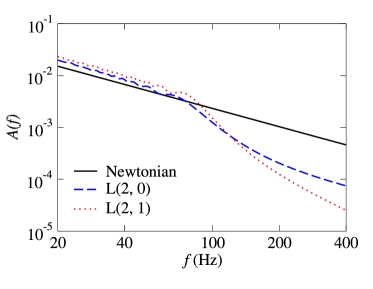
Figure 11: Frequency-domain amplitude versus frequency for the L-approximated (restricted) waveforms, at different PN orders, for a $(15+15)M_{\odot}$ BBH.

Definition of the models

For these models, just as for the HT and HP models, the choice of the endpoint of evolution is rather arbitrary. We decided to stop the integration of the dynamical equations when we begin to observe unphysical effects due to the failure of the PN expansion. For many (if not all) configurations, the PN-expanded center-of-mass binding energy (given by Eqs. (2.7a)–(2.7e) of Ref. kidder ) begins to increase during the late inspiral, instead of continuing to decrease. When this happens, we stop the integration. The instantaneous GW frequency at that time will then be the ending frequency for these waveforms. We shall refer to these models as ${\rm L}(n{\rm PN},m{\rm PN})$, where $n{\rm PN}$ ($n{\rm PN}$) denotes the maximum PN order of the terms included in the Hamiltonian (the radiation-reaction force). We shall consider $(n{\rm PN},m{\rm PN})=(2,0),(2,1)$.

Waveforms and matches

In Fig. 11, we plot the frequency-domain amplitude versus frequency for the L-approximated (restricted) waveforms, at different PN orders, for a $(15+15)M_{\odot}$ BBH. The amplitude deviates from the Newtonian prediction slightly before $100$ Hz. Indeed, the GW ending frequencies are $116$ Hz and $107$ Hz for the L$(2,0)$ and L$(2,1)$ models, respectively. These frequencies are quite low, because the unphysical behavior of the PN-expanded center-of-mass binding energy appears quite early [at $r_{\rm end}=6.6$ and $r_{\rm end}=7.0$ for the L$(2,0)$ and L$(2,1)$ models, respectively]. So the L models do not provide waveforms for the last stage of inspirals and plunge.

Table IV.2 shows the maxmax matches between the L-approximants and a few other selected PN models. The overlaps are quite high, except with the EP$(2,2.5)$ and EP$(3,3.5,0)$ at high masses, but extremely unfaithful. Moreover, we could expect the L$(2,0)$ and L$(2,1)$ models to have high fitting factors with the adiabatic models T$(2,0)$ and T$(2,1)$. However, this is not the case. As Table IV.2 shows, the T models are neither effectual nor faithful in matching the L models, and vice versa. This might be due to one of the following factors: (i) the PN-expanded conservative dynamics in the adiabatic limit (T models) and in the nonadiabatic case (L models) are rather different; (ii) there is an important effect due to the different criteria used to end the evolution in the two models, which make the ending frequencies rather different. All in all, the L models do not seem very reliable, so we shall not give them much credit when we discuss detection template families. However, we shall investigate where they lie in the detection template space.

		T(2, 2)			T(3, 3.5, 0)			P(2, 2.5)			P(3, 3.5, 0)			EP(2, 2.5)			EP(3, 3.5, 0)			HT(3, 3.5, 0)
		mm	$M$	$\eta$	mm	$M$	$\eta$	mm	$M$	$\eta$	mm	$M$	$\eta$	mm	$M$	$\eta$	mm	$M$	$\eta$	mm	$M$	$\eta$
L(2, 1)	(20+20)$M_{\odot}$	$0.994$	$78.83$	$0.05$	$0.998$	$61.24$	$0.09$	$0.999$	$52.76$	$0.13$	$0.998$	$57.96$	$0.11$	$0.935$	$70.76$	$0.05$	$0.9446$	$72.04$	$0.06$	$0.994$	$49.53$	$0.14$
	(15+15)$M_{\odot}$	$0.991$	$55.16$	$0.06$	$0.995$	$44.50$	$0.10$	$0.999$	$39.96$	$0.13$	$0.998$	$43.57$	$0.11$	$0.912$	$46.67$	$0.09$	$0.916$	$50.90$	$0.07$	$0.994$	$37.08$	$0.15$
	(15+5)$M_{\odot}$	$0.981$	$35.51$	$0.05$	$0.991$	$29.03$	$0.08$	$0.995$	$26.02$	$0.10$	$0.994$	$27.99$	$0.09$	$0.942$	$27.46$	$0.09$	$0.941$	$28.85$	$0.08$	$0.994$	$22.89$	$0.13$
	(5+5)$M_{\odot}$	$0.956$	$10.68$	$0.20$	$0.965$	$11.49$	$0.18$	$0.971$	$11.33$	$0.19$	$0.964$	$11.89$	$0.17$	$0.964$	$11.03$	$0.19$	$0.960$	$11.69$	$0.17$	$0.966$	$11.32$	$0.18$

Table 6: Fitting factors [see Eq. (20)] for the projection of the L$(2,1)$ (target) waveforms onto the T, P, EP and HP (search) models at 2PN and 3PN order. The values quoted are obtained by maximizing the maxmax (mm) match over the search-model parameters $M$ and $\eta$.

		L$(2,0)$			T$(2,0)$			L$(2,1)$			T$(2,1)$
		mm	$M$	$\eta$	mm	$M$	$\eta$	mm	$M$	$\eta$	mm	$M$	$\eta$
	(15+15)$M_{\odot}$				0.884	42.02	0.237
L$(2,0)$	(15+5)$M_{\odot}$				0.769	24.71	0.201
	(5+5)$M_{\odot}$				0.996	21.70	0.068
	(15+15)$M_{\odot}$	0.834	23.44	0.247
T$(2,0)$	(15+5)$M_{\odot}$	0.823	14.90	0.250
	(5+5)$M_{\odot}$	0.745	9.11	0.250
	(15+15)$M_{\odot}$										0.837	60.52	0.236
L$(2,1)$	(15+5)$M_{\odot}$										0.844	55.70	0.052
	(5+5)$M_{\odot}$										0.626	11.47	0.238
	(15+15)$M_{\odot}$							0.663	19.38	0.250
T$(2,1)$	(15+5)$M_{\odot}$							0.672	13.56	0.250
	(5+5)$M_{\odot}$							0.631	9.22	0.243

Table 7: Fitting factors [see Eq. (20)] for the projection of the L$(2,1)$ and L$(2,0)$ (target) waveforms onto the T$(2,0)$ and T$(2,1)$ (search) models. The values quoted are obtained by maximizing the maxmax (mm) match over the search-model parameters $M$ and $\eta$.

IV.3 Nonadiabatic PN resummed methods: the Effective-One-Body approach

The basic idea of the effective-one-body (EOB) approach BD1 is to map the real two-body conservative dynamics, generated by the Hamiltonian (56) and specified up to 3PN order, onto an effective one-body problem where a test particle of mass $\mu=m_{1}m_{2}/M$ (with $m_{1}$ and $m_{2}$ the BH masses, and $M=m_{1}+m_{2}$) moves in an effective background metric $g_{\mu\nu}^{\rm eff}$ given by

$$ds_{\rm eff}^{2}\equiv g_{\mu\nu}^{\rm eff}\,dx^{\mu}\,dx^{\nu}=-A(R)\,c^{2}dt^{2}+\frac{D(R)}{A(R)}\,dR^{2}+R^{2}\,(d\theta^{2}+\sin^{2}\theta\,d\varphi^{2})\,,$$ (80)

where

$$A(R) = 1+a_{1}\,\frac{GM}{c^{2}R}+a_{2}\left(\frac{GM}{c^{2}R}\right)^{2}+a_{3}\left(\frac{GM}{c^{2}R}\right)^{3}+a_{4}\left(\frac{GM}{c^{2}R}\right)^{4}+\cdots\,,$$ (81)

$$D(R) = 1+d_{1}\,\frac{GM}{c^{2}R}+d_{2}\left(\frac{GM}{c^{2}R}\right)^{2}+d_{3}\left(\frac{GM}{c^{2}R}\right)^{3}+\cdots\,.$$ (82)

The motion of the particle is described by the action

$$S_{\rm eff}=-\mu c\int ds_{\rm eff}\,.$$ (83)

For the sake of convenience, in this section we shall use the same symbols of Secs. IV.1 and  IV.2 to denote different physical quantities (such as coordinates in different gauges). The mapping between the real and the effective dynamics is worked out within the Hamilton–Jacobi formalism, by imposing that the action variables of the real and effective description coincide (i.e., ${J_{\rm real}}={J_{\rm eff}}$, ${{\cal I}_{\rm real}}={{\cal I}_{\rm eff}}$, where $J$ denotes the total angular momentum, and ${\cal I}$ the radial action variable BD1 ), while allowing the energy to change,

$$\frac{{\cal E}_{\rm eff}^{\rm NR}}{\mu c^{2}}=\frac{{\cal E}_{\rm real}^{\rm NR}}{\mu c^{2}}\left[1+\alpha_{1}\,\frac{{\cal E}_{\rm real}^{\rm NR}}{\mu c^{2}}+\alpha_{2}\left(\frac{{\cal E}_{\rm real}^{\rm NR}}{\mu c^{2}}\right)^{2}+\alpha_{3}\left(\frac{{\cal E}_{\rm real}^{\rm NR}}{\mu c^{2}}\right)^{3}+\cdots\right]\,,$$ (84)

here ${\cal E}^{\rm NR}_{\rm eff}$ is the Non–Relativistic effective energy, while is related to the relativistic effective energy ${\cal E}_{\rm eff}$ by the equation ${\cal E}^{\rm NR}_{\rm eff}={\cal E}_{\rm eff}-\mu\,c^{2}$; ${\cal E}_{\rm eff}$ is itself defined uniquely by the action (83). The Non–Relativistic real energy ${\cal E}_{\rm real}^{\rm NR}\equiv H({\bf q},{\bf p})$, where $H({\bf q},{\bf p})$ is given by Eq. (56) with $H({\bf q},{\bf p})=\mu\widehat{H}({\bf q},{\bf p})$. From now on, we shall relax our notation and set $G=c=1$.

Equations of motion

Damour, Jaranowski and Schäfer EOB3PN found that, at 3PN order, this matching procedure contains more equations to satisfy than free parameters to solve for ($a_{1},a_{2},a_{3},d_{1},d_{2},d_{3}$, and $\alpha_{1},\alpha_{2},\alpha_{3}$). These authors suggested the following two solutions to this conundrum. At the price of modifying the energy map and the coefficients of the effective metric at the 1PN and 2PN levels, it is still possible at 3PN order to map uniquely the real two-body dynamics onto the dynamics of a test mass moving on a geodesic (for details, see App. A of Ref. EOB3PN ). However, this solution appears very complicated; more importantly, it seems awkward to have to compute the 3PN Hamiltonian as a foundation for deriving the matching at the 1PN and 2PN levels. The second solution is to abandon the hypothesis that the effective test mass moves along a geodesic, and to augment the Hamilton–Jacobi equation with (arbitrary) higher-derivative terms that provide enough coefficients to complete the matching. With this procedure, the Hamilton-Jacobi equation reads

$$0=\mu^{2}+g_{\rm eff}^{\mu\eta}(x)\,p_{\mu}\,p_{\eta}+A^{\mu\eta\rho\sigma}(x)\,p_{\mu}\,p_{\eta}\,p_{\rho}\,p_{\sigma}+\cdots\,.$$ (85)

Because of the quartic terms $A^{\alpha\beta\gamma\delta}$, the effective 3PN relativistic Hamiltonian is not uniquely fixed by the matching rules defined above; the general expression is EOB3PN :

$$\mathcal{E}^{\mathrm{NR}}_{\mathrm{eff}}\equiv\widehat{H}_{\rm eff}({\mathbf{q}},{\mathbf{p}})=\sqrt{A(q)\left[1+{\mathbf{p}}^{2}+\left(\frac{A(q)}{D(q)}-1\right)({\mathbf{n}}\cdot{\mathbf{p}})^{2}+\frac{1}{q^{2}}\left(z_{1}({\mathbf{p}}^{2})^{2}+z_{2}\,{\mathbf{p}}^{2}({\mathbf{n}}\cdot{\mathbf{p}})^{2}+z_{3}({\mathbf{n}}\cdot{\mathbf{p}})^{4}\right)\right]}\,,$$ (86)

here we use the reduced relativistic effective Hamiltonian $\widehat{H}_{\rm eff}={H}_{\rm eff}/\mu$, and ${\bf q}$ and ${\bf p}$ are the reduced canonical variables, obtained by rescaling the canonical variables by $M$ and $\mu$, respectively. The coefficients $z_{1},z_{2}$ and $z_{3}$ are arbitrary, subject to the constraint

$$8z_{1}+4z_{2}+3z_{3}=6(4-3\eta)\,\eta\,.$$ (87)

Moreover, we slightly modify the EOB model at 3PN order of Ref. EOB3PN by requiring that in the test mass limit the 3PN EOB Hamiltonian equal the Schwarzschild Hamiltonian. Indeed, one of the original rationales of the PN resummation methods was to recover known exact results in the test-mass limit. To achieve this, $z_{1},z_{2}$ and $z_{3}$ must go to zero as $\eta\rightarrow 0$. A simple way to enforce this limit is to set $z_{1}=\eta\tilde{z}_{1},z_{2}=\eta\tilde{z}_{2}$ and $z_{3}=\eta\tilde{z}_{3}$. With this choice the coefficients $A(r)$ and $D(r)$ in Eq. (86) read:

$$A(r) = 1-\frac{2}{r}+\frac{2\eta}{r^{3}}+\left[\left(\frac{94}{3}-\frac{41}{32}\pi^{2}\right)-\tilde{z}_{1}\right]\,\frac{\eta}{r^{4}}\,,$$ (88)

$$D(r) = 1-\frac{6\eta}{r^{2}}+\left[7\tilde{z}_{1}+\tilde{z}_{2}+2(3\eta-26)\right]\,\frac{\eta}{r^{3}}\,,$$ (89)

where we set $r=|{\bf q}|$. The authors of Ref. EOB3PN restricted themselves to the case ${z}_{1}={z}_{2}=0$ ($\tilde{z}_{1}=\tilde{z}_{2}=0$). Indeed, they observed that for quasicircular orbits the terms proportional to $z_{2}$ and $z_{3}$ in Eq. (86) are very small, while for circular orbits the term proportional to $z_{1}$ contributes to the coefficient $A(r)$, as seen in Eq. (88). So, if the coefficient $z_{1}=\eta\tilde{z}_{1}\neq 0$, its value could be chosen such as to cancel the 3PN contribution in $A(r)$. To avoid this fact, which can be also thought as a gauge effect due to the choice of the coordinate system in the effective description, the authors of Ref. EOB3PN decided to pose ${z}_{1}=0$ ($\tilde{z}_{1}=0$). By contrast, in this paper we prefer to explore the effect of having $z_{1,2}\neq 0$. So we shall depart from the general philosophy followed by the authors in Ref. EOB3PN , pushing (or expanding) the EOB approach to more extreme regimes.

Now, the reduction to the one-body dynamics fixes the arbitrary coefficients in Eq. (84) uniquely to $\alpha_{1}=\eta/2$, $\alpha_{2}=0$, and $\alpha_{3}=0$, and provides the resummed (improved) Hamiltonian [obtained by solving for ${\cal E}_{\rm real}^{\rm NR}$ in Eq. (84) and imposing $H^{\rm improved}\equiv{\cal E}_{\rm real}^{\rm NR}$]:

$$H^{\rm improved}=M\,\sqrt{1+2\eta\,\left(\frac{H_{\rm eff}-\mu}{\mu}\right)}\,.$$ (90)

Including radiation-reaction effects, we can then write the Hamilton equations in terms of the reduced quantities $\widehat{H}^{\rm improved}=H^{\rm improved}/\mu$, $\widehat{t}=t/M$, $\widehat{\omega}=\omega\,M$ BD2 ,

$$\frac{dr}{d\widehat{t}} = \frac{\partial\widehat{H}^{\rm improved}}{\partial p_{r}}(r,p_{r},p_{\varphi})\,,$$ (91)

$$\frac{d\varphi}{d\widehat{t}} \equiv \widehat{\omega}=\frac{\partial\widehat{H}^{\rm improved}}{\partial p_{\varphi}}(r,p_{r},p_{\varphi})\,,$$ (92)

$$\frac{dp_{r}}{dt} = -\frac{\partial\widehat{H}^{\rm improved}}{\partial r}(r,p_{r},p_{\varphi})\,,$$ (93)

$$\frac{dp_{\varphi}}{d\widehat{t}} = \widehat{F}^{\varphi}[\widehat{\omega}(r,p_{r},p_{\varphi})]\,,$$ (94)

where for the $\varphi$ component of the radiation-reaction force we use the T- and P-approximants to the flux function [see Eqs. (63), (64)]. Note that at each PN order, say $n$PN, we integrate the Eqs. (91)–(94) without further truncating the partial derivatives of the Hamiltonian at $n$PN order (differentiation with respect to the canonical variables can introduce terms of order higher than $n$PN).

Following the discussion around Eq. (67), the ISCO of these models is determined by setting $\partial H_{0}^{\rm improved}/\partial r=\partial^{2}H_{0}^{\rm improved}/\partial r^{2}=0$, where $H_{0}^{\rm improved}(r,p_{r},p_{\varphi})=H^{\rm improved}(r,0,p_{\varphi})$. If we define

$$\widehat{H}_{\rm eff}^{2}(r,0,p_{\varphi})\equiv W_{p_{\varphi}}=A(r)\,\left(1+\frac{p_{\varphi}^{2}}{r^{2}}+\eta\,\tilde{z}_{1}\,\frac{p_{\varphi}^{4}}{r^{6}}\right)\,,$$ (95)

we extract the ISCO by imposing $\partial W_{p_{\varphi}}(r)/\partial r=0=\partial^{2}W_{p_{\varphi}}(r)/\partial^{2}r$. Damour, Jaranowski and Schäfer EOB3PN noticed that at 3PN order, for $\tilde{z}_{1}=\tilde{z}_{2}=0$, and using the PN expanded form for $A(r)$ given by Eq. (88), there is no ISCO. To improve the behavior of the PN expansion of $A(r)$ and introduce an ISCO, they proposed replacing $A(r)$ with the Padé approximants

$$A_{P_{2}}(r)=\frac{r(-4+2r+\eta)}{2r^{2}+2\eta+r\eta}\,,$$ (96)

and

$$A_{P_{3}}(r)=\frac{r^{2}[(a_{4}(\eta,0)+8\eta-16)+r(8-2\eta)]}{r^{3}\,(8-2\eta)+r^{2}\,(a_{4}(\eta,0)+4\eta)+r\,(2a_{4}(\eta,0)+8\eta)+4(\eta^{2}+a_{4}(\eta,0))}\,,$$ (97)

where

$$a_{4}(\eta,\tilde{z}_{1})=\left[\frac{94}{3}-\frac{41}{32}\pi^{2}-\tilde{z}_{1}\right]\,\eta\,.$$ (98)

In Table 2, we show the GW frequency at the ISCO for some typical choices of BBH masses, computed using the above expressions for $A(r)$ in the improved Hamiltonian (90) with $\tilde{z}_{1}=\tilde{z}_{2}=0$.

We use the Padé resummation for $A(r)$ of Ref. EOB3PN also for the general case $\tilde{z}_{1}\neq 0$, because for the PN expanded form of $A(r)$ the ISCO does not exist for a wide range of values of $\tilde{z}_{1}$. [However, when we discuss Fourier-domain detection template families in Sec. VI, we shall investigate also EOB models with PN-expanded $A(r)$.]

In Fig. 12, we plot the binding energy as evaluated using the improved Hamiltonian (90), at different PN orders, for equal-mass BBHs. At 3PN order, we use as typical values $\tilde{z}_{1}=0,\pm 4$. [For $\tilde{z}_{1}>4$ the location of the ISCO is no longer a monotonic function of $\tilde{z}_{1}$. So we set $\tilde{z}_{1}\leq 4$.] In the right panel of Fig. 12, we show the variation in the GW frequency at the ISCO as a function of $\tilde{z}_{1}$ for a (15+15)$M_{\odot}$ BBH.

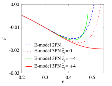
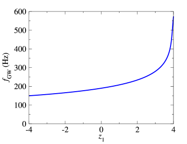
Figure 12: In the left panel, we plot the binding energy evaluated using the improved Hamiltonian (90), as a function of the velocity parameter $v$, for equal-mass BBHs, $\eta=0.25$. We plot different PN orders for the E-model varying also the parameter $\tilde{z}_{1}$. In the right panel, we plot the GW frequency at the ISCO at 3PN order as a function of the parameter $\tilde{z}_{1}$ for (15+15)$M_{\odot}$ BBH.

Finally, in Fig. 13, we compare the binding energy for a few selected PN models, where for the E models we fix $\tilde{z}_{1}=\tilde{z}_{2}=0$ [see the left panel of Fig. 12 for the dependence of the binding energy on the coefficient $\tilde{z}_{1}$]. Notice, in the left panel, that the 2PN and 3PN T energies are much closer to each other than the 2PN and 3PN P energies are, and than the 2PN and 3PN E energies are; notice also that the 3PN T and P energies are very close. The closeness of the binding energies (and of the MECOs and ISCOs) predicted by PN expanded and resummed models at 3PN order (with $\tilde{z}_{1}=0$), and of the binding energy predicted by the numerical quasiequilibrium BBH models of Ref. GGB was recently pointed out in Refs. LB ; DGG . However, the EOB results are very close to the numerical results of Ref. GGB only if the range of variation of $\tilde{z}_{1}$ is restricted.

Definition of the models

For these models, we use the initial conditions laid down in Ref. DIS2 , and also adopted in this paper for the HT and HP models (see Sec. IV.1). At 2PN order, we stop the integration of the Hamilton equations at the light ring given by the solution of the equation $r^{3}-3r^{2}+5\eta=0$ BD2 . At 3PN order, the light ring is defined by the solution of

$$\frac{d}{du}\left[u^{2}\,A_{P_{3}}(u)\right]=0,$$ (99)

with $u=1/r$ and $A_{P_{3}}$ is given by Eq. (97). For some configurations, the orbital frequency and the binding energy start to decrease before the binary can reach the 3PN light ring, so we stop the evolution when $\dot{\hat{\omega}}=0$ [see discussion in Sec. IV.4 below]. For other configurations, it happens that the radial velocity becomes comparable to the angular velocity before the binary reaches the light ring; in this case, the approximation used to introduce the RR effects into the conservative dynamics is no longer valid, and we stop the integration of the Hamilton equations when $|\dot{r}/(r\dot{\varphi})|$ reaches $0.3$. For some models, usually those with $\tilde{z}_{1,2}\neq 0$, the quantity $|\dot{r}/(r\dot{\varphi})|$ reaches a maximum during the last stages of evolution, then it starts decreasing, and $\dot{r}$ becomes positive. In such cases, we choose to stop at the maximum of $|\dot{r}/(r\dot{\varphi})|$.

In any of these cases, the instantaneous GW frequency at the time when the integration is stopped defines the ending frequency for these waveforms.

We shall refer to the EOB models (E-approximants) as ${\rm ET}(n{\rm PN},m{\rm PN})$ (when the T-approximant is used for the flux) or ${\rm EP}(n{\rm PN},m{\rm PN})$ (when the P-approximant is used for the flux), where $n{\rm PN}$ ($m{\rm PN}$) denotes the maximum PN order of the terms included in the Hamiltonian (flux). We shall consider $(n{\rm PN},m{\rm PN})=(1,1.5)$, $(2,2.5)$, and $(3,3.5,\hat{\theta})$ [at 3PN order we need to indicate also a choice of the arbitrary flux parameter $\hat{\theta}$].

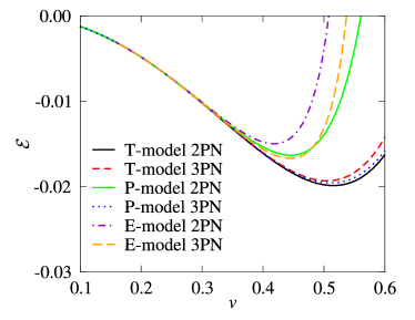
Figure 13: Binding energy as a function of the velocity parameter $v$, for equal-mass BBHs. We plot different PN orders for selected PN models. For the E model at 3PN order we fix $\tilde{z}_{1}=0=\tilde{z}_{2}$.

Waveforms and matches

In Table IV.2, we investigate the dependence of the E waveforms on the values of the unknown parameters $\tilde{z}_{1}$ and $\tilde{z}_{2}$ that appear in the EOB Hamiltonian at 3PN order. The coefficients $\tilde{z}_{1}$ and $\tilde{z}_{2}$ are in principle completely arbitrary. When $\tilde{z}_{1}\neq 0$, the location of the ISCO changes, as shown in Fig. 12. Moreover, because in Eq. (86) $\tilde{z}_{1}$ multiplies a term that is not zero on circular orbits, the motion tends to become noncircular much earlier, and the criteria for ending the integration of the Hamilton equations are satisfied earlier. [See the discussion of the ending frequency in the previous section.] This effect is much stronger in equal-mass BBHs with high $M$. For example, for (15+15)$M_{\odot}$ BBHs and for $\tilde{z}_{2}=0$, the fitting factor (the maxmax match, maximized over $M$ and $\eta$) between an EP target waveform with $\tilde{z}_{1}=0$ and EP search waveforms with $-40\,\raise 1.72218pt\hbox{$<$}\kern-8.00003pt\lower 2.6694pt\hbox{$\sim$}\,\tilde{z}_{1}<-4$ can well be $\leq\,0.9$. However, if we restrict $\tilde{z}_{1}$ to the range $[-4,4]$, we get very high fitting factors, as shown in Table IV.2.

In Eq. (86), the coefficients $\tilde{z}_{2}$ and $\tilde{z}_{3}$ multiply terms that are zero on circular orbits. [The coefficient $\tilde{z}_{2}$ appears also in $D(r)$, given by Eq. (89).] So their effect on the dynamics is not very important, as confirmed by the very high matches obtained in Table IV.2 between EP waveforms with $\tilde{z}_{2}=0$ and EP waveforms with $\tilde{z}_{2}=\pm 4$. It seems that the effect of changing $\tilde{z}_{2}$ is nearly the same as a remapping of the BBH mass parameters.

We investigated also the case in which we use the PN expanded form for $A(r)$ given by Eq. (88). For example, for (15+15)$M_{\odot}$ BBHs and $\tilde{z}_{2}=0$, the fitting factors between EP target waveforms with $\tilde{z}_{1}=-40,-4,4,40$ and EP search waveforms with $\tilde{z}_{1}=0$ are $({\rm maxmax},M,\eta)=(0.767,39.55,0.240)$, $(0.993,30.83,0.241)$, $(0.970,30.03,0.241)$, and $(0.915,28.23,0.242)$, respectively. So the overlaps can be quite low.

In Table 8, for three typical choices of BBH masses, we perform a convergence test using Cauchy’s criterion. The values are quite high. However, as for the P-approximants, we have no way to test whether the E-approximants are converging to the true limit. In Fig. 14, we plot the frequency-domain amplitude of the EP-approximated (restricted) waveforms, at different PN orders, for a (15 +15)$M_{\odot}$ BBH. The evolution of the EOB models contains a plunge characterized by quasicircular motion BD2 . This plunge causes the amplitude to deviate from the Newtonian amplitude, $\mathcal{A}_{\mathrm{Newt}}=f^{-7/6}$ around $200$ Hz, which is a higher frequency than we found for the adiabatic models [see Figs. 4, 7].

In Table IV.2, for some typical choices of the masses, we evaluate the fitting factors between the ET$(2,2.5)$ and ET$(3,3.5)$ waveforms (with $\tilde{z}_{1}=\tilde{z}_{2}=0$) and the $\mathrm{T}(2,2.5)$ and $\mathrm{T}(3,3.5)$ waveforms. This comparison should emphasize the effect of moving from the adiabatic orbital evolution, ruled by the energy-balance equation, to the (almost) full Hamiltonian dynamics, ruled by the Hamilton equations. More specifically, we see the effect of the differences in the conservative dynamics between the PN expanded T-model and the PN resummed E-model (the radiation-reaction effects are introduced in the same way in both models). While the matches are quite low at 2PN order, they are high ($\geq 0.95$) at 3PN order, at least for $M\leq 30M_{\odot}$, but the estimation of $m_{1}$ and $m_{2}$ is poor. This result suggests that, for the purpose of signal detection as opposed to parameter estimation, the conservative dynamics predicted by the EOB resummation and by the PN expansion are very close at 3PN order, at least for $M\leq 30M_{\odot}$. Moreover, the results of Table IV.2 suggest also that the effect of the unknown parameter $\hat{\theta}$ is rather small, at least if $\hat{\theta}$ is of order unity, so in the following we shall always set $\hat{\theta}=0$.

In Tables IV.2 and IV.2 we study the difference between the EP$(2,2.5)$ and EP$(3,3.5)$ models (with $\tilde{z}_{1}=\tilde{z}_{2}$=0), and all the other adiabatic and nonadiabatic models. For some choices of BBH masses, these tables show the maxmax matches between the search models in the columns and the target models in the rows, maximized over the search-model parameters $M$ and $\eta$, with the restriction $0<\eta\leq 1/4$. At 2PN order, the matches with the T$(2,2.5)$, HT$(2,2)$ and HP$(2,2.5)$ models are low, while with the matches with the T$(2,2)$ and P$(2,2.5)$ models are high, at least for $M\leq 30M_{\odot}$ (but the estimation of the BH masses is poor). At 3PN order, the matches with T$(3,3.5,\hat{\theta})$, P$(3,3.5,\hat{\theta})$, HP$(3,3.5,\hat{\theta})$ and HT$(3,3.5,\hat{\theta})$ are quite high if $M\leq 30M_{\odot}$. However, for $M=40M_{\odot}$, the matches can be quite low. We expect that this happens because in this latter case the differences in the late dynamical evolution become crucial.

$N$	$\left<{\rm EP}_{N},{\rm EP}_{N+1}\right>$
	$(5+20)M_{\odot}$	$(10+10)M_{\odot}$				$(15+15)M_{\odot}$
0	0.677	0.584	(0.769,	17.4,	0.246)	0.811
1	0.766	0.771	(0.999,	21.8,	0.218)	0.871
2 ($\hat{\theta}=+2$)	0.862	0.858	(0.999,	21.3,	0.222)	0.898
2 ($\hat{\theta}=-2$)	0.912	0.928	(0.999,	21.9,	0.211)	0.949

Table 8: Test for the Cauchy convergence of the EP-approximants. The values quoted assume optimization on the extrinsic parameters but the same intrinsic parameters (i.e., they assume the same masses). Here we define $\mathrm{EP}_{0}=\mathrm{EP}(0,0)$, $\mathrm{EP}_{1}=\mathrm{EP}(1,1.5)$, $\mathrm{EP}_{2}=\mathrm{EP}(2,2.5)$, and $\mathrm{EP}_{3}=\mathrm{EP}(3,3.5,\hat{\theta},\tilde{z}_{1}=\tilde{z}_{2}=0)$. The values in parentheses are the maxmax matches obtained by maximizing with respect to the extrinsic and intrinsic parameters, shown together with the $\mathrm{EP}_{N+1}$ parameters $M$ and $\eta$ where the maxima are attained. In all cases the integration of the equations is started at a GW frequency of $20$ Hz.

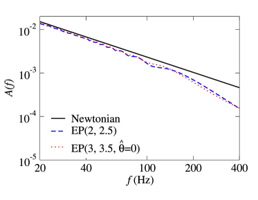
Figure 14: Frequency-domain amplitude versus frequency for the EP-approximated (restricted) waveform, at different PN orders, for a $(15+15)M_{\odot}$ BBH.

IV.4 Features of the late dynamical evolution in nonadiabatic models

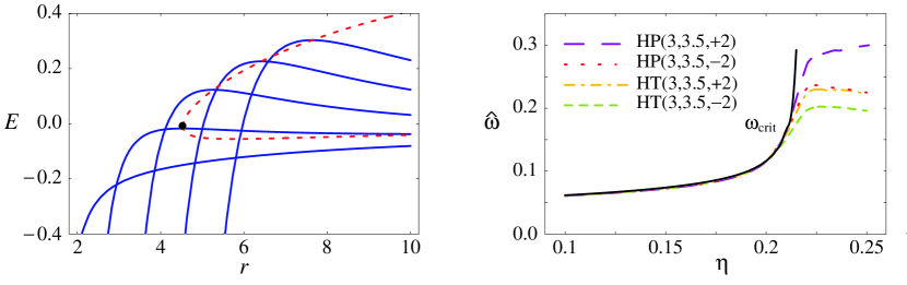
Figure 15: Ending points of the H models at 3PN order for low values of $\eta$. In the left panel, we plot as a function of $r$ the Hamiltonian $\widehat{H}(r,p_{r}=0,p_{\varphi})$ [given by Eq. (56)], evaluated at $\eta=0.16$ for a (5+20)$M_{\odot}$ BBH, for various values of the (reduced) angular momentum $p_{\varphi}$. The circular-orbit solutions are found at the values of $r$ and $\hat{H}$ joined by the dashed line. At $r_{\rm crit}=4.524$ there is a critical radius, below which there is no circular orbit. In the right panel, we plot as a function of $\eta$ the orbital angular frequency $\widehat{\omega}_{\rm crit}(\eta)$ corresponding to the critical radius, for $0.1<\eta<0.21$ (solid line). This curve agrees well with the ending frequencies of the HT and HP models at 3PN order, which are shown as dotted and dashed lines in the figure.

While studying the numerical evolution of nonadiabatic models, we encounter two kinds of dynamical behavior that are inconsistent with the assumption of quasicircular motion used to include the radiation-reaction effects, so when one of these two behaviors occurs, we immediately stop the integration of the equations of motion. First, in the late stage of evolution $\widehat{\omega}$ can reach a maximum, and then drop quickly to zero; so we stop the integration if $\dot{\widehat{\omega}}=0$. Second, the radial velocity $\dot{r}$ can become a significant portion of the total speed, so we stop the integration if $\dot{r}=0.3(r\widehat{\omega})$.

The first behavior is found mainly in the H models at 3PN order, when $\eta$ is relatively small ($\stackrel{{\scriptstyle<}}{{{}_{\sim}}}0.21$). As we shall see below, it is not characteristic of either the Schwarzschild Hamiltonian or the EOB Hamiltonian. In the left panel of Fig. 15, we plot the binding energy evaluated from $\widehat{H}(r,p_{r}=0,p_{\varphi})$ [given by Eq. (56)] as a function of $r$ at $\eta=0.16$, for various values of the (reduced) angular momentum $p_{\varphi}$. As this plot shows, there exists a critical radius, $r_{\rm crit}$, below which no circular orbits exist. This $r_{\mathrm{crit}}$ can be derived as follows. From Fig. 15 (left), we deduce that

$$\left.{{\frac{d\widehat{H}}{dr}}}\right|_{\rm circ}\rightarrow\infty\,,\quad\quad r\rightarrow r_{\rm crit}\,.$$ (100)

Because circular orbits satisfy the conditions

$$p_{r}=0\,,\quad\quad\frac{\partial\widehat{H}}{\partial r}=0\,,$$ (101)

and

$$\left.{{\frac{dp_{\varphi}}{dr}}}\right|_{\rm circ}=-\frac{\partial^{2}\widehat{H}}{\partial r^{2}}\,\left(\frac{\partial^{2}\widehat{H}}{\partial r\partial p_{\varphi}}\right)^{-1}\,,$$ (102)

we get

$$\left.{{\frac{d\widehat{H}}{dr}}}\right|_{\rm circ}=\left.\frac{\partial\widehat{H}}{\partial r}+\frac{\partial\widehat{H}}{\partial p_{\varphi}}\,{{\frac{dp_{\varphi}}{dr}}}\right|_{\rm circ}=-\frac{\partial\widehat{H}}{\partial p_{\varphi}}\,\frac{\partial^{2}\widehat{H}}{\partial r^{2}}\,\left(\frac{\partial^{2}\widehat{H}}{\partial r\partial p_{\varphi}}\right)^{-1}\,.$$ (103)

Combining these equations we obtain two conditions that define $r_{\mathrm{crit}}$:

$$\left.\frac{\partial\widehat{H}}{\partial r}\right|_{r_{\mathrm{crit}}}=0\,,\quad\quad\left.\frac{\partial^{2}\widehat{H}}{\partial r\partial p_{\varphi}}\right|_{r_{\mathrm{crit}}}=0\,.$$ (104)

In the right panel of Fig. 15, we plot the critical orbital frequency $\widehat{\omega}_{\rm crit}$ as a function of $\eta$ in the range [0.1, 0.21]. In the same figure, we show also the ending frequencies for the HT$(3,3.5,\pm 2)$ and HP$(3,3.5,\pm 2)$ models. For $0.1<\eta<0.21$, these ending frequencies are in good agreement with the critical frequencies $\hat{\omega}_{\mathrm{crit}}$; for $\eta>0.21$, the ending condition $\dot{r}=0.3(r\widehat{\omega})$ is satisfied before $\dot{\hat{\omega}}=0$. For $0.1<\eta<0.21$, this good agreement can be explained as follows: for the H models at 3PN order with $\eta\stackrel{{\scriptstyle<}}{{{}_{\sim}}}0.21$, the orbital evolution is almost quasicircular (i.e., $\dot{r}$ remains small and $\widehat{\omega}$ keeps increasing) until the critical point is reached; beyond this point, there is no way to keep the orbit quasicircular, as the angular motion is converted significantly into radial motion, and $\widehat{\omega}$ begins to decrease. This behavior ($\dot{\widehat{\omega}}\rightarrow 0$) is also present in the E model in the vicinity of the light ring, because the light ring is also a minimal radius for circular orbits [the conditions (100) are satisfied also in this case]. However, the behavior of the energy is qualitatively different for the H and E models: in the E models (just as for a test particle in Schwarzchild spacetime) the circular-orbit energy goes to infinity, while this is not the case for the H models.

The second behavior is usually caused by radiation-reaction effects, and accelerated by the presence of an ISCO (and therefore of a plunge). However, it is worth to mention another interesting way in which the criterion $\dot{r}=0.3(r\hat{\omega})$ can be satisfied for some E evolutions at 3PN order. During the late stages of evolution, $\dot{r}$ sometimes increases suddenly and drastically, and the equations of motion become singular. This behavior is quite different from a plunge due to the presence of an ISCO (in that case the equations of motion do not become singular). The cause of this behavior is that at 3PN order the coefficient $D(r)$ [see Eq. (89)] can go to zero and become negative for a sufficiently small $r$. For $\tilde{z}_{1}=\tilde{z}_{2}=0$, this occurs at the radius $r_{D}$ given by

$$r_{\rm D}^{3}-6\eta r_{\rm D}+2(3\eta-26)\eta=0;$$ (105)

$r_{D}$ can fall outside the light ring. For example, for $\eta=0.25$ we have $r_{\rm D}=2.54$, while the light rings sits at $r=2.31$. On the transition from $D(r)>0$ to $D(r)<0$, the effective EOB metric unphysical, and the E model then becomes invalid. Using the Hamiltonian equation of motion (91), it is straightforward to prove that a negative $D(r)$ causes the radial velocity to blow up:

$$\dot{r}=\frac{\partial\widehat{H}}{\partial p_{r}}\propto\frac{p_{r}}{D(r)}\rightarrow\infty\quad\quad{\rm as}\quad r\rightarrow r_{\rm D}\,.$$ (106)

V Signal-to-noise ratio for the two-body models

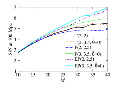
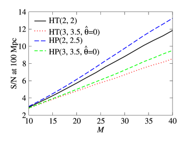
Figure 16: Signal-to-noise ratio at 100 Mpc versus total mass $M$, for selected PN models. The S/N is computed for equal-mass BBHs using the LIGO-I noise curve (28) and the waveform expression (29) with the rms $\Theta=8/5$; for the E model at 3PN we set $\tilde{z}_{1}=\tilde{z}_{2}=0$.

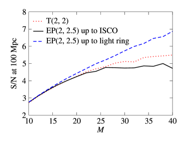
Figure 17: Effect of the plunge on the signal-to-noise ratio. The S/N is computed at 100 Mpc for equal-mass BBHs, as a function of the total mass, for the T$(2,2)$ adiabatic model (for comparison), and for the EP$(2,2.5)$ model with ending frequency at the ISCO, and at the light ring (in this latter case the signal includes a plunge). Here we use the LIGO-I noise curve (28) and the waveform expression (29) with the rms $\Theta=8/5$.

In Fig. 16, we plot the optimal signal-to-noise ratio $\rho_{\mathrm{opt}}$ for a few selected PN models. The value of $\rho_{\mathrm{opt}}$ is computed using Eqs. (1) and (19) with the waveform given by Eq. (29), for a luminosity distance of 100 Mpc and the rms $\Theta=8/5$ [see discussion around Eq. (29)]; for the EP model we set $\tilde{z}_{1}=\tilde{z}_{2}=0$. Notice that, because the E models have a plunge, their signal-to-noise ratios are much higher (at least for $M\geq 30M_{\odot}$) than those for the adiabatic models, which we cut off at the MECO. See also Fig. 17, which compares the S/N for EP$(2,2.5)$ waveforms with and without the plunge; for $M=20M_{\odot}$, excluding the plunge decreases the S/N by $\sim$ 4% (which corresponds to a decrease in detection rate of 12% for a fixed detection threshold); while for $M=30M_{\odot}$, excluding the plunge decreases the S/N by $\sim$ 22% (which corresponds to a decrease in detection rate of 54%). This result confirms the similar conclusion drawn in Ref. DIS3 .

Because at 2PN and 3PN order the H models do not have a plunge, but the two BHs continue to move on quasicircular orbits even at close separations, the number of total GW cycles is increased, and so is the signal-to-noise ratio, as shown in the right panel of Fig. 16. However, we do not trust the H models much, because they show a very different behavior at different PN orders, as already emphasized in Sec. IV.1.

VI Performance of Fourier-domain detection templates, and construction of a Fourier-domain detection-template bank

In the previous sections we have seen [for instance, in Table IV.2] that the overlaps between the various PN waveforms are not very high, and that there could be an important loss in event rate if, for the purpose of detection, we restricted ourselves to only one of the two-body models [see Figs. 16, 17]. To cope with this problem we propose the following strategy. We guess that the conjunction of the waveforms from all the PN models spans a region in signal space that includes (or almost includes) the true signals, and we build a detection template family that embeds all the PN models in a higher-dimensional space. The PN models that we have considered (expanded and resummed, adiabatic and nonadiabatic) rely on a wide variety of very different dynamical equations, so the task of consolidating them under a single set of generic equations seems arduous. On the other hand, we have reason to suspect, from the values of the matches, and from direct investigations, that the frequency-domain amplitude and phasing (the very ingredients that enter the determination of the matches) are, qualitatively, rather similar functions for all the PN models. We shall therefore create a family of templates that model directly the Fourier transform of the GW signals, by writing the amplitude and phasing as simple polynomials in the GW frequency $f_{\mathrm{GW}}$. We shall build these polynomials with the specific powers of $f_{\mathrm{GW}}$ that appear in the Fourier transform of PN expanded adiabatic waveforms, as computed in the stationary-phase approximation. However, we shall not constrain the coefficients of these powers to have the same functional dependence on the physical parameters that they have in that scheme. More specifically, we define our generic family of Fourier-domain effective templates as

$$h_{\rm eff}(f)={\cal A}_{\rm eff}(f)\,e^{i\psi_{\rm eff}(f)}\,,$$ (107)

where

$${\cal A}_{\rm eff}(f) = f^{-7/6}\,\left(1-\alpha\,f^{2/3}\right)\,\theta(f_{\rm cut}-f)\,,$$ (108)

$${\psi}_{\rm eff}(f) = 2\pi ft_{0}+\phi_{0}+f^{-5/3}\,\left(\psi_{0}+\psi_{1/2}\,f^{1/3}+\psi_{1}\,f^{2/3}+\psi_{3/2}\,f+\psi_{2}\,f^{4/3}+\cdots\right)\,,$$ (109)

where $t_{0}$ and $\phi_{0}$ are the time of arrival and the frequency-domain phase offset, and where $\theta(\ldots)$ is the Heaviside step function. This detection template family is similar in some respects to the template banks implicitly used in Fast Chirp Transform techniques JP . However, because we consider BBHs with masses $10\mbox{--}40M_{\odot}$, the physical GW signal can end within the LIGO frequency band; and the predictions for the ending frequency given by different PN models can be quite different. Thus, we modify also the Newtonian formula for the amplitude, by introducing the cutoff frequency $f_{\rm cut}$ and the shape parameter $\alpha$.

The significance of $f_{\rm cut}$ with respect to true physical signals deserves some discussion. If the best match for the physical signal $g$ is the template $h_{f_{\mathrm{cut}}}$, which ends at the instantaneous GW frequency $f_{\mathrm{cut}}$ (so that $h_{f_{\mathrm{cut}}}(f)\simeq g(f)$ for $f<f_{\mathrm{cut}}$ and $h_{f_{\mathrm{cut}}}(f)=0$ for $f>f_{\mathrm{cut}}$), then we can be certain to lose a fraction of the optimal $\rho$ that is given approximately by

$$\frac{\rho_{\mathrm{cut}}}{\rho_{\mathrm{opt}}}\leq\frac{\sqrt{\int_{0}^{f_{\mathrm{cut}}}\frac{|\tilde{g}(f)|^{2}}{S_{n}(f)}df}}{\sqrt{\int_{0}^{\infty}\frac{|\tilde{g}(f)|^{2}}{S_{n}(f)}df}}\simeq 1-\frac{1}{2}\frac{\int_{f_{\mathrm{cut}}}^{\infty}\frac{|\tilde{g}(f)|^{2}}{S_{n}(f)}df}{\int_{0}^{\infty}\frac{|\tilde{g}(f)|^{2}}{S_{n}(f)}df}.$$ (110)

On the other hand, if we try to match $g$ with the same template family without cuts (and if indeed the $h$’s are completely inadequate at modeling the amplitude and phasing of $g$ above $f_{\mathrm{cut}}$), then even the best-match template $h_{\mathrm{no\,cut}}$ (defined by $h_{\mathrm{no\,cut}}(f)\simeq g(f)$ for $f<f_{\mathrm{cut}}$, and by zero correlation, $\overline{h_{\mathrm{no\,cut}}(f)g^{*}(f)}\simeq 0$ for $f>f_{\mathrm{cut}}$) will yield an additional loss in $\rho$ caused by the fact that we are spreading the power of the template beyond the range where it can successfully match $g$. Mathematically, this loss comes from the different normalization factor for the templates $h_{f_{\mathrm{cut}}}$ and $h_{\mathrm{no\,cut}}$, and it is given by

$$\frac{\rho_{\mathrm{no\,cut}}}{\rho_{\mathrm{cut}}}\leq\frac{\sqrt{\int_{0}^{f_{\mathrm{cut}}}\frac{|\tilde{h}(f)|^{2}}{S_{n}(f)}df}}{\sqrt{\int_{0}^{\infty}\frac{|\tilde{h}(f)|^{2}}{S_{n}(f)}df}}\simeq 1-\frac{1}{2}\frac{\int_{f_{\mathrm{cut}}}^{\infty}\frac{|\tilde{h}(f)|^{2}}{S_{n}(f)}df}{\int_{0}^{\infty}\frac{|\tilde{h}(f)|^{2}}{S_{n}(f)}df}.$$ (111)

If we assume that $g$ and $h_{\mathrm{no\,cut}}$ have roughly the same amplitude distribution, the two losses are similar.

In the end, we might be better off cutting templates if we cannot be sure that their amplitude and phasing, beyond a certain frequency, are faithful representations of the true signal. Doing so, we approximately halve the worst-case loss of $\rho$, because instead of losing a factor

$$\frac{\rho_{\mathrm{no\,cut}}}{\rho_{\mathrm{cut}}}\frac{\rho_{\mathrm{cut}}}{\rho_{\mathrm{opt}}}\simeq 1-\frac{1}{2}\frac{\int_{f_{\mathrm{cut}}}^{\infty}\frac{|\tilde{h}(f)|^{2}}{S_{n}(f)}df}{\int_{0}^{\infty}\frac{|\tilde{h}(f)|^{2}}{S_{n}(f)}df}-\frac{1}{2}\frac{\int_{f_{\mathrm{cut}}}^{\infty}\frac{|\tilde{g}(f)|^{2}}{S_{n}(f)}df}{\int_{0}^{\infty}\frac{|\tilde{g}(f)|^{2}}{S_{n}(f)}df}\simeq 1-\frac{\int_{f_{\mathrm{cut}}}^{\infty}\frac{|\tilde{g}(f)|^{2}}{S_{n}(f)}df}{\int_{0}^{\infty}\frac{|\tilde{g}(f)|^{2}}{S_{n}(f)}df},$$ (112)

we lose only the factor $\rho_{\mathrm{cut}}/\rho_{\mathrm{opt}}$. On the other hand, we do not want to lose the signal-to-noise ratio that is accumulated at high frequencies if our templates have a fighting chance of matching the true signal there; so it makes sense to include in the detection bank the same template with several different values of $f_{\mathrm{cut}}$.

It turns out that using only the two parameters $\psi_{0}$ and $\psi_{3/2}$ in the phasing (and setting all other $\psi$ coefficients to zero) and the two amplitude parameters, $f_{\rm cut}$ and $\alpha$, we obtain a family that can already match all the PN models of Secs. III, IV with high fitting factors FF. This is possible largely because we restrict our focus to BBHs with relatively high masses, where the number of GW cycles in the LIGO range (and thus the total range of the phasing $\psi(f)$ that we need to consider) is small.

In Tab. LABEL:tableETB1 we list the minmax (see Sec. II) fitting factor for the projection of the PN models onto our frequency-domain effective templates, for a set of BBH masses ranging from $(5+5)M_{\odot}$ to $(20+20)M_{\odot}$. In computing the fitting factors, we used the simplicial search algorithm amoeba nrc to search for the optimal set of parameters $(\psi_{0},\,\psi_{3/2},\,f_{\rm cut},\,\alpha)$ (as always, the time of arrival and initial phase of the templates were automatically optimized as described in Sec. II). From Tab. LABEL:tableETB1 we draw the following conclusions:

1. All the adiabatic models (T and P) are matched with fitting factors $\mathrm{FF}>0.97$. Lower-mass BBHs are matched better than higher-mass BBHs, presumably because for the latter the inspiral ends at lower frequencies within the LIGO band, producing stronger edge effects, which the effective templates cannot capture fully. 3PN models are matched better than 2PN models.

2. The Effective-One-Body models (ET and EP) are matched even better than the adiabatic models, presumably because they have longer inspirals and less severe edge effects at the end of inspiral. Unlike the adiabatic models, however, ET and EP are matched better for higher-mass BBHs. In fact, all the FFs are $>0.99$ except for $(5+5)M_{\odot}$ BBHs, where $\mathrm{FF}\gtrsim 0.979$. The reason for this is probably that this low-mass BBH has more GW cycles in the LIGO frequency band than any other one, and the two phasing parameters of our effective templates cannot quite model the evolution of the phasing. [In the adiabatic models, these effects may be overshadowed by the loss in signal to noise ratio due to the edge effects at high frequencies.] When the parameters $\tilde{z}_{1,2}$ are allowed to be nonzero, the matches get worse, but not by much. For all the plausible values of $\tilde{z}_{1}$, the worst situation seems to happen at $\tilde{z}_{1}=-40$, where the overlaps are still higher than $\sim 0.95$ [with minimum 0.947.]

3. The Hamiltonian models (HT and HP) at 3PN order are not matched as precisely, but the detection template family still works reasonably well. We usually have $\mathrm{FF}>0.96$, but there are several exceptions, with FF as low as 0.948. For these models, the overlaps are lower in the equal-mass cases, where the ending frequencies of the waveforms are much higher than for the other models; it seems that the effective templates are not able to reproduce this late portion of the waveforms (this might not be so bad, because it does not seem likely that this part of the signal reflects the true behavior of BBH waveforms).

4. The Lagrangian models (L) are matched a bit worse than the Hamiltonian models (HT and HP) at 3PN, but they still have $\mathrm{FF}$ higher than $0.95$ in most cases, with several exceptions [at either $(20+20)M_{\odot}$ or $(5+5)M_{\odot}$], which can be as low as $0.93$.

5. HT and HP models at 2PN are matched the worst, with typical values lower than $0.95$ and higher than $0.85$.

Finally, we note that our amplitude function ${\cal A}_{\rm eff}(f)$ is a linear combination of two terms, so we can search automatically over the correction coefficient $\alpha$, in essentially the same way as discussed in Sec. II for the orbital phase. In other words, $\alpha$ is an extrinsic parameter. [Although we do search over $\alpha$, it is only to show the required range, which will be a useful piece of information when one is deciding how to lay down a mesh of discrete templates on the continuous detection-template space.]

VI.1 Internal match and metric

To understand the matches between the Fourier-domain templates and the PN models, and to prepare to compute the number of templates needed to achieve a given (internal) MM, we need to derive an expression for the match between two Fourier-domain effective templates.

We shall first restrict our consideration to effective templates with the same amplitude function (i.e., the same $\alpha$ and $f_{\rm cutoff}$). The overlap $\langle h(\psi_{0},\psi_{3/2}),h(\psi_{0}+\Delta\psi_{0},\psi_{3/2}+\Delta\psi_{3/2})\rangle$ between templates with close values of $\psi_{0}$ and $\psi_{3/2}$ can be described (to second order in $\Delta\psi_{0}$ and $\Delta\psi_{3/2}$) by the mismatch metric $g_{ij}$ O :

$$\langle h(\psi_{0},\psi_{3/2}),h(\psi_{0}+\Delta\psi_{0},\psi_{3/2}+\Delta\psi_{3/2})\rangle=1-\sum_{i,j=0,3/2}g_{\rm ij}\,\Delta\psi_{i}\Delta\psi_{j}.$$ (113)

The metric coefficients $g_{ij}$ can be evaluated analytically from the overlap

$$\langle h(\psi_{0},\psi_{3/2}),h(\psi_{0}+\Delta\psi_{0},\psi_{3/2}+\Delta\psi_{3/2})\rangle\simeq$$

$$\left[\max_{\Delta\phi_{0},\Delta t_{0}}\int df\frac{|{\cal A}{(f)}|^{2}}{S_{h}(f)}\cos\left(\sum_{i}\frac{\Delta\psi_{i}}{f^{n_{i}}}+\Delta\phi_{0}+2\pi f\Delta t_{0}\right)\right]\Bigg{/}\left[\int df\frac{|{\cal A}{(f)}|^{2}}{S_{h}(f)}\right]\simeq$$

$$1-\frac{1}{2}\left[\max_{\Delta\phi_{0},\Delta t_{0}}\int df\frac{|{\cal A}{(f)}|^{2}}{S_{h}(f)}\left(\sum_{i}\frac{\Delta\psi_{i}}{f^{n_{i}}}+\Delta\phi_{0}+2\pi f\Delta t_{0}\right)^{2}\right]\Bigg{/}\left[\int df\frac{|{\cal A}{(f)}|^{2}}{S_{h}(f)}\right].$$ (114)

where $n_{0}\equiv 5/3$ and $n_{3/2}\equiv 2/3$. Comparison with Eq. (113) then gives

$$\sum_{i,j}g_{\rm ij}\,\Delta\psi_{i}\Delta\psi_{j}=\frac{1}{2}\min_{\Delta\phi_{0},\Delta t_{0}} \left\{\left(\begin{array}[]{cc}\Delta\psi_{0}&\Delta\psi_{3/2}\end{array}\right){\bf M}_{(1)}\left(\begin{array}[]{c}\Delta\psi_{0}\\ \Delta\psi_{3/2}\end{array}\right)\right.+$$ (125)

$$\left.2\left(\begin{array}[]{cc}\Delta\phi_{0}&2\pi\Delta t_{0}\end{array}\right){\bf M}_{(2)}\left(\begin{array}[]{c}\Delta\psi_{0}\\ \Delta\psi_{3/2}\end{array}\right)+\left(\begin{array}[]{cc}\Delta\phi_{0}&2\pi\Delta t_{0}\end{array}\right){\bf M}_{(3)}\left(\begin{array}[]{c}\Delta\phi_{0}\\ 2\pi\Delta t_{0}\end{array}\right)\right\}$$

where the ${\bf M}_{(1)\ldots(3)}$ are the matrices

$${\bf M}_{(1)} = \left[\begin{array}[]{cc}J(2n_{0})&J(n_{0}+n_{3/2})\\ J(n_{0}+n_{3/2})&J(2n_{3/2})\end{array}\right]\,,$$ (128)

$${\bf M}_{(2)} = \left[\begin{array}[]{cc}J(n_{0})&J(n_{3/2})\\ J(n_{0}-1)&J(n_{3/2}-1)\end{array}\right]\,,$$ (131)

$${\bf M}_{(3)} = \left[\begin{array}[]{cc}J(0)&J(-1)\\ J(-1)&J(-2)\end{array}\right]\,,$$ (134)

and where

$$J(n)\equiv\left[\int df\frac{|{\cal A}(f)|^{2}}{S_{h}(f)}\frac{1}{f^{n}}\right]\bigg{/}\left[\int df\frac{|{\cal A}(f)|^{2}}{S_{h}(f)}\right]\,.$$ (135)

Since ${\bf M}_{(3)}$ describes the mismatch caused by $(\Delta\phi_{0},\Delta t_{0})$, it must be positive definite; because the right-hand side of (125) reaches its minimum with respect to variations of $\Delta\phi_{0}$ and $\Delta t_{0}$ when

$$2{\bf M}_{(2)}\left(\begin{array}[]{c}\Delta\psi_{0}\\ \Delta\psi_{3/2}\end{array}\right)+2{\bf M}_{(3)}\left(\begin{array}[]{c}\Delta\phi_{0}\\ 2\pi\Delta t_{0}\end{array}\right)=0\,,$$ (136)

we obtain

$$g_{\rm ij}=\frac{1}{2}\left[{\bf M}_{(1)}-{\bf M}_{(2)}^{\rm T}{\bf M}_{(3)}^{-1}{\bf M}_{(2)}\right]_{ij}\,.$$ (137)

We note also that the mismatch $\langle h(\psi_{0},\psi_{3/2}),h(\psi_{0}+\Delta\psi_{0},\psi_{3/2}+\Delta\psi_{3/2})\rangle$ is translationally invariant in the $(\psi_{0},\psi_{3/2})$ plane, so the metric $g_{ij}$ is constant everywhere.

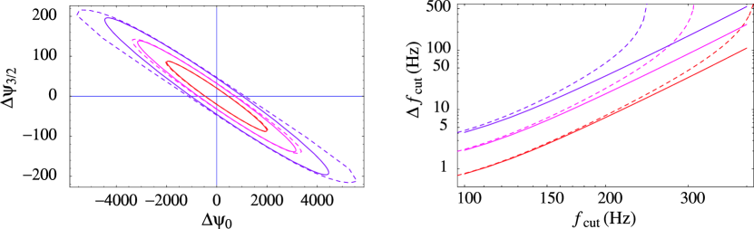
Figure 18: In the left panel, we plot the iso-match contours for the function $\langle h(\psi_{0},\psi_{3/2}),h(\psi_{0}+\Delta\psi_{0},\psi_{3/2}+\Delta\psi_{3/2})\rangle$; contours are given at matches of 0.99, 0.975 and 0.95. Solid lines give the indications of the mismatch metric; dashed lines give actual values. Here we use a Newtonian amplitude function ${\cal A}(f)=f^{-7/6}$ [we set $\alpha=0$ and we do not cut the template in the frequency domain. In fact $f_{\mathrm{cut}}=400\,\mathrm{Hz}$]. In the right panel we plot the values of $\Delta f_{\mathrm{cut}}$ (versus $f_{\rm cut}$) required to obtain matches $\langle h(f_{\mathrm{cut}}),h(f_{\mathrm{cut}}+\Delta f_{\mathrm{cut}})\rangle$ of 0.95 (uppermost curve), 0.975 and 0.99 (lowermost). In the region below each contour the match is larger than the value quoted for the contour. Again, here we use a Newtonian amplitude function ${\cal A}(f)=f^{-7/6}$ [we set $\alpha=0$].

In the left panel of Fig. 18, we plot the iso-match contours (at matches of 0.99, 0.975 and 0.95) in the $(\Delta\psi_{0},\Delta\psi_{3/2})$ plane, as given by the metric (137) [solid ellipses], compared with the actual values obtained from the numerical computation of the matches [dashed lines]. For our purposes, the second-order approximation given by the metric is quite acceptable. In this computation we use a Newtonian amplitude function ${\cal A}(f)=f^{-7/6}$ [i.e., we set $\alpha=0$ and we set our cutoff frequency at $400\,\mathrm{Hz}$].

We move now to the mismatch induced by different cutoff frequencies $f_{\mathrm{cut}}$. Unlike the case of the $\psi_{0}$, $\psi_{3/2}$ parameters, this mismatch is first order in $\Delta f_{\rm cut}$, so it cannot be described by a metric. Suppose that we have two effective templates $h(f_{\mathrm{cut}})$ and $h(f_{\mathrm{cut}}+\Delta f_{\mathrm{cut}})$ with the same phasing and amplitude $\Delta f>0$, but different cutoff frequencies. The match is then given by

$$\langle h(f_{\rm cut}),h(f_{\rm cut}+\Delta f_{\mathrm{cut}})\rangle = \frac{\left[\int_{0}^{f_{\rm cut}}df\frac{|{\cal A}(f)|^{2}}{S_{h}(f)}\right]}{\left[\int_{0}^{f_{\rm cut}}df\frac{|{\cal A}(f)|^{2}}{S_{h}(f)}\right]^{1/2}\left[\int_{0}^{f_{\rm cut}+\Delta f_{\mathrm{cut}}}df\frac{|{\cal A}(f)|^{2}}{S_{h}(f)}\right]^{1/2}}$$ (138)

$$= \left[\frac{\int_{0}^{f_{\rm cut}}df\frac{|{\cal A}(f)|^{2}}{S_{h}(f)}}{\int_{0}^{f_{\rm cut}+\Delta f_{\mathrm{cut}}}df\frac{|{\cal A}(f)|^{2}}{S_{h}(f)}}\right]^{1/2}\,\simeq 1-\left[\frac{\Delta f_{\mathrm{cut}}}{2}\frac{|{\cal A}(f_{\mathrm{cut}})|^{2}}{S_{h}(f_{\mathrm{cut}})}\right]\bigg{/}\left[\int_{0}^{f_{\rm cut}}df\frac{|{\cal A}(f)|^{2}}{S_{h}(f)}\right]^{1/2}\,.$$ (139)

This result depends strongly on $f_{\mathrm{cut}}$. In the right panel of Fig. 18 we plot the values of $\Delta f_{\mathrm{cut}}$ that correspond to matches of 0.95, 0.975 and 0.99, according to the first order approximation [solid lines], and to the exact numerical calculations [dashed lines], both of which are given in the second line of Eq. (139). In the region below each contour the match is larger than the value that characterizes the contour. As we can see from the graph, the linear approximation is not very accurate, thus in the following we shall use the exact formula.

VI.2 Construction of the effective template bank: parameter range

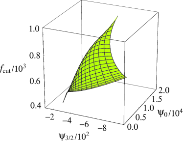
Figure 19: Projection of the ET$(2,2.5)$ waveforms onto the frequency-domain effective template space. For $\alpha$ we choose the optimal value found by the search. The $(\psi_{0},\psi_{3/2},f_{\rm cut})$ surface is interpolated from the then mass pairs shown in Tab. LABEL:tableETB1.

All the PN target models are parametrized by two independent numbers (e.g., the two masses or the total mass and the mass ratio); if we select a range of interest for these parameters, the resulting set of PN signals can be seen as a two-dimensional region in the $(m_{1},m_{2})$ or $(M,\eta)$ plane. Under the mapping that takes each PN signal into the Fourier-domain effective template that matches it best, this two-dimensional region is projected into a two-dimensional surface in the $(\psi_{0},\psi_{3/2},f_{\mathrm{cut}})$ parameter space (with the fourth parameter $\alpha=0$). As an example, we show in Fig. 19 the projection of the ET$(2,2.5)$ waveforms with (single-BH) masses $5$–$20\,{\rm M}_{\odot}$. The 26 models tested in Secs. III, IV would be projected into 26 similar surfaces. In constructing the detection template families, we shall first focus on 17 of the 26 models, namely the adiabatic T and P models at 2PN and 3PN, the E models at 2PN and at 3PN but with $\tilde{z}_{1,2}=0$, and the H models at 3PN. We will comment on the E models with $\tilde{z}_{1,2}\neq 0$, on the L models, and on the HT and HP models at 2PN order at the end of this section.

It is hard to visualize all three parameters at once, so we shall start with the phasing parameters $\psi_{0}$ and $\psi_{3/2}$. In Fig. 20, we plot the $(\psi_{0},\psi_{3/2})$ section of the PN-model projections into the ($\psi_{0},\psi_{3/2},f_{\rm cutoff})$ space, with solid diamonds showing the projected points corresponding to BBHs with the same set of ten mass pairs as in Tab. LABEL:tableETB1. Each PN model is projected to a curved-triangular region, with boundaries given by the sequences of BBHs with masses $(m+m)$ (equal mass), $(20+m)$ and $(m+5)$. In Fig. 20, these boundaries are plotted using thin dashed lines, for the models T$(2,2.5)$ (the uppermost in the plot), HT$(3,3.5,\hat{\theta}=2)$ (in the middle), and P$(2,2.5)$ (lowest).

As we can see, different PN models can occupy regions with very different areas, and thus require a very different number of effective templates to match them with a given $\mathrm{MM}_{\mathrm{T}}$. Among these three models, T$(2,2.5)$ requires the least number of templates, P$(2,2.5)$ requires a few times more, and HT$(3,3.5,\hat{\theta}=2)$ requires many more. This is consistent with the result by Porter P02 who found that, for the same range of physical parameters, T waveforms are more closely spaced than P waveforms, so fewer are needed to achieve a certain MM. In this plot we have also linked the points that correspond to the same BBH parameters in different PN models. In Fig. 20, these lines (we shall call them BH mass lines) lie all roughly along one direction.

$M$	end-to-end match	${\cal N}_{\rm end\,to\,end}$	$f_{\rm cut\,min}$	$\langle h(f_{\rm cut\,min}),h(+\infty)\rangle$	${\cal N}_{\rm mass\,line}^{\rm cut}$
$(5+5)M_{\odot}$	0.478	37	572	1.00	0.2
$(10+5)M_{\odot}$	0.434	41	346	0.98	0.9
$(15+5)M_{\odot}$	0.398	46	232	0.94	3.1
$(10+10)M_{\odot}$	0.449	40	246	0.95	2.6
$(20+5)M_{\odot}$	0.347	52	192	0.90	5.3
$(15+10)M_{\odot}$	0.443	40	226	0.94	3.3
$(20+10)M_{\odot}$	0.428	42	185	0.89	5.9
$(15+15)M_{\odot}$	0.482	36	191	0.90	5.4
$(20+15)M_{\odot}$	0.464	38	162	0.84	8.5
$(20+20)M_{\odot}$	0.438	41	143	0.79	11.9

Table 9: End-to-end matches and ending frequencies along the BH mass lines of Fig. 20. The first three columns show the end-to-end matches and the corresponding number of templates (for MM $\simeq 0.98$) along the BH mass lines; the remaining columns show the minimum ending frequencies of PN waveforms along the BH mass lines, the match between the two effective templates at the ends of the range, and the number of templates needed to step along the range while always maintaining a match $\simeq 0.98$ between neighboring templates. When computing these matches, we use a Newtonian amplitude function ${\cal A}(f)=f^{-7/6}$ [we set $\alpha=0$], and we maximize over the parameters $\psi_{0}$ and $\psi_{3/2}$ (which is equivalent to assuming perfect phasing synchronization).

A simple way to characterize the difference between the PN target models is to evaluate the maxmax end-to-end match between effective templates at the two ends of the BH mass lines (i.e., the match between the effective templates with the largest and smallest $\psi_{3/2}$ among the projections of PN waveforms with the same mass parameters $m_{1}$, $m_{2}$); we wish to focus first on the effects of the phasing parameters, so we do not cut the templates in the frequency domain and we set $\alpha=0$. We compute also a naive end-to-end number of templates, ${\cal N}_{\mathrm{end\,to\,end}}$, by counting the templates required to step all along the BH mass line while maintaining at each step a match $\simeq 0.98$ between neighboring templates. A simple computation yields ${\cal N}_{\mathrm{end\,to\,end}}=\log(\mbox{end-to-end match})/\log(0.98)$. The results of this procedure are listed in Table 9. Notice that, as opposed to the fitting factors between template families computed elsewhere in this paper (which are maximized over the BBH mass parameters of one of the families), these matches give a measure of the dissimilarity between different PN models for the same values of the BBH parameters; thus, they provide a crude estimate of how much the effective template bank must be enlarged to embed all the various PN models.

We expect that the projection of a true BBH waveform onto the $(\psi_{0},\psi_{3/2})$ plane will lie near the BH mass line with the true BBH parameters, or perhaps near the extension of the BH mass line in either direction. For this reason we shall lay down our effective templates in the region traced out by the thick dashed lines in Fig. 20, which was determined by extending the BH mass lines in both directions by half of their length.

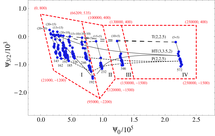
Figure 20: Projection of the PN waveforms onto the ($\psi_{0}$,$\psi_{3/2}$) plane, for BBHs with masses $(5+5)M_{\odot}$, $(10+5)M_{\odot}$, …, $(20+20)M_{\odot}$ (see Tab. LABEL:tableETB1). The projection was computed by maximizing the maxmax match over the parameters $\psi_{0}$, $\psi_{3/2}$ and $f_{\mathrm{cut}}$; the correction coefficient $\alpha$ was set to zero. The thin dotted and dashed lines show the boundaries of the projected images for the models (from the top) T$(2,2.5)$, HT$(3,3.5,\hat{\theta}=2)$ and P$(2,2.5)$. Solid lines (the BH mass lines) link the images of the same BBH for different PN models. The ends of the BH mass lines are marked with the BBH masses and with the minimum value $\min\{f_{\mathrm{end}},f_{\mathrm{cut}}\}$ across all the PN models. The thick dashed lines delimit the region that will be covered by the effective template bank; the $(\psi_{0},\psi_{3/2})$ coordinates are marked on the vertices. The region is further subdivided into four subregions I–IV that group the BH mass lines with very similar ending frequencies $f_{\mathrm{end\,min}}$.

We move on to specifying the required range of $f_{\rm cut}$ for each $(\psi_{0},\psi_{3/2})$. For a given PN model and BBH mass parameters, we have defined the ending frequency $f_{\mathrm{end}}$ as the instantaneous GW frequency at which we stop the integration of the PN orbital equations. We find that usually the $f_{\rm cut}$ of the optimally-matched projection of a PN template is larger than the $f_{\mathrm{end}}$ of the PN template. This is because the abrupt termination of the PN waveforms in the time domain creates a tail in the spectrum for frequencies higher than $f_{\mathrm{end}}$. With $f_{\mathrm{cut}}>f_{\mathrm{end}}$ and $\alpha>0$, the effective templates can mimic this tail and gain a higher match with the PN models. In some cases, however, the optimal $f_{\rm cut}$ can be smaller than $f_{\rm end}$ [for example, P$(2,2.5)$ with $(10+5)M_{\odot}$, $(15+5)M_{\odot}$ and $(10+10)M_{\odot}$] suggesting that the match of the phasing in the entire frequency band up to $f_{\rm end}$ is not very good and we have to shorten the Fourier-domain template. Now, since we do not know the details of the plunge for true BBH inspiral, it is hard to estimate where the optimal $f_{\mathrm{cut}}$ might lie, except perhaps imposing that it should be larger than ${\rm min}(f_{\mathrm{end}},f_{\mathrm{cut}})$. A possibility is to set the range of $f_{\mathrm{cut}}$ to be above $f_{\rm cut\,min}\equiv\min\{f_{\mathrm{cut}},f_{\mathrm{end}}\}$, with the minimum evaluated among all the PN models.

In Table 9 we show the $f_{\mathrm{cut\,min}}$ found across the PN models for given BBH mass parameters. We have also marked this minimum frequency in Fig. 20 under the corresponding BH mass lines. In the table we also show the match of the two detection templates $h(f_{\mathrm{cut}}=f_{\mathrm{cut\,min}})$ and $h(f_{\mathrm{cut}}=+\infty)$, and the number ${\cal N}^{\mathrm{cut}}_{\mathrm{mass\,line}}$ of intermediate templates with different $f_{\mathrm{cut}}$ needed to move from $h(f_{\mathrm{cut\,min}})$ to $h(+\infty)$ while maintaining at each step a match $\simeq 0.98$ between neighboring templates. It is easy to see that this number is ${\cal N}^{\mathrm{cut}}_{\mathrm{mass\,line}}=\log\langle h(f_{\rm cut\,min}),h(+\infty)\rangle/\log(0.98)$. The match was computing using a Newtonian amplitude function ${\cal A}(f)=f^{-7/6}$ [we set $\alpha=0$], and maximizing over the parameters $\psi_{0}$ and $\psi_{3/2}$. Under our previous hypothesis that the projection of a true BBH waveform would lie near the corresponding BH mass line, we can use the numbers in Table 9 to provide a rough estimate of the range of $f_{\mathrm{cut}}$ that should be taken at each point $(\psi_{0},\psi_{3/2})$ within the dashed contour of Fig. 20. We trace out four subregions I, II, III, IV, such that the BH mass lines of each subregion have approximately the same values of $f_{\rm cut\,min}$; we then use these minimum ending frequencies to set a lower limit for the values of $f_{\mathrm{cut}}$ required in each subregion: $f_{\mathrm{cut\,min}}(\mathrm{I})=143$, $f_{\mathrm{cut\,min}}(\mathrm{II})=192$, $f_{\mathrm{cut\,min}}(\mathrm{III})=232$, $f_{\mathrm{cut\,min}}(\mathrm{IV})=346$. The maximum $f_{\mathrm{cut}}$ is effectively set by the detector noise curve, which limits the highest frequency at which signal-to-noise can be still accumulated.

Moving on to the last parameter, $\alpha$, we note that it is probably only meaningful to have $\alpha f_{\mathrm{cut}}^{2/3}\leq 1$, so that $\mathcal{A}_{\mathrm{eff}}(f)$ cannot become negative for $f<f_{\mathrm{cut}}$. [A negative amplitude in the detection template will usually give a negative contribution to the overlap, unless the phasing mismatch is larger than $\pi/2$, which does not seem plausible in our cases.] Indeed, the optimized values found for $\alpha$ in Tab. LABEL:tableETB1 seem to follow this rule, except for a few slight violations that are probably due to numerical error (since we had performed a search to find the optimal value of $\alpha$). For the 17 models considered here, the optimal $\alpha$ is always positive [Tab. LABEL:tableETB1] which means that, due to cutoff effects, the amplitude at high frequencies becomes always lower than the $f^{-7/6}$ power law. So for the 17 models considered in this section $0\leq\alpha f_{\mathrm{cut}}^{2/3}\leq 1$. [Note that this range will have to be extended to include negative $\alpha$’s if we want to incorporate the models discussed in Sec. VI.5.]

VI.3 Construction of the effective templates bank: parameter density

At this stage, we have completed the specification of the region in the $(\psi_{0},\psi_{3/2},f_{\rm cut},\alpha)$ parameter space where we shall lay down our bank of templates. We expect that the FF for the projection of the true physical signals (emitted by nonspinning BBHs with $M=10\mbox{--}40M_{\odot}$) onto this template bank should be very good. We now wish to evaluate the total number of templates $\mathcal{N}$ needed to achieve a certain MM.

We shall find it convenient to separate the mismatch due to the phasing from the mismatch due to the frequency cuts by introducing two minimum match parameters $\mathrm{MM}_{\psi}$ and $\mathrm{MM}_{\mathrm{cut}}$, with $\mathrm{MM}=\mathrm{MM}_{\psi}\cdot\mathrm{MM}_{\mathrm{cut}}\simeq\mathrm{MM}_{\psi}+\mathrm{MM}_{\mathrm{cut}}-1$. As mentioned at the beginning of this section, the correction coefficient $\alpha$ is essentially an extrinsic parameter [see Sec. II.2]: we do not need to discretize the template bank with respect to $\alpha$, and there is no corresponding $\mathrm{MM}$ parameter.

We evaluate $\mathcal{N}$ in three refinement steps:

1. We start by considering only the phasing parameters, and we compute the parameter area $S_{i}$ [in the $(\psi_{0},\psi_{3/2})$ plane] for each of the subregions $i=$ I, II, III, IV of Fig. 20. We then multiply by the determinant $\sqrt{g}$ of the constant metric, and divide by 2(1–MM_ψ), according to Eq. (25), to get

   $$\mathcal{N}=\sum_{i}\frac{S_{i}\sqrt{g}}{2(1-\mathrm{MM}_{\psi})}.$$ (140)

   This expression is for the moment only formal, because we cannot compute $\sqrt{g}$ without considering the amplitude parameters $\alpha$ and $f_{\mathrm{cut}}$.

2. Next, we include the effect of $f_{\mathrm{cut}}$. In the previous section, we have set $f_{\mathrm{min\,cut}}$ for each of the subregions by considering the range swept by $f_{\mathrm{end}}$ along the mass lines. Recalling our discussion of $\mathcal{N}^{\mathrm{cut}}_{\mathrm{mass\,line}}$, we approximate the number of distinct values of $f_{\mathrm{cut}}$ that we need to include for each parameter pair $(\psi_{0},\psi_{3/2})$ as

   $$n^{\mathrm{cut}}_{i}(\psi_{0},\psi_{3/2},\alpha)\simeq 1+\frac{\log\left\langle h(\psi_{0},\psi_{3/2},\alpha,f_{\mathrm{min\,cut}}),h(\psi_{0},\psi_{3/2},\alpha,\mathrm{no\,cut})\right\rangle}{\log\mathrm{MM}_{\mathrm{cut}}}.$$ (141)

   For $\alpha$ in the physical range $0\leq\alpha\leq f^{-2/3}_{\mathrm{cut}}$ this match is minimized for $\alpha=0$, so this is the value that we use to evaluate the $n^{\mathrm{cut}}_{i}$’s. Note that the choice of cutoff frequencies does not depend on the values of the phasing parameters. This allows us to have a single set of cutoff frequencies for all points in one subregion. For subregion $i$, we denote this set by $F_{i}$.

3. The final step is to include the effect of $\alpha$ and $f_{\mathrm{cut}}$ on the computation of $\sqrt{g}$. For simplicity, we shoot for an upper limit by maximizing $\sqrt{g}$ with respect to $\alpha$. [Because $\alpha$ is essentially an extrinsic parameter, we do not multiply $\mathcal{N}$ by the number of its discrete values: the matches are automatically maximized on the continuous range $0\leq\alpha\leq f_{\mathrm{cut}}^{-2/3}$.] Our final estimate for the total number of templates is

   $$\mathcal{N}=\frac{1}{2(1-\mathrm{MM}_{\psi})}\sum_{i}S_{i}\sum_{f_{\mathrm{cut}}\in F_{i}}\max_{\alpha}[\sqrt{g}]$$ (142)

We have evaluated this $\mathcal{N}$ numerically. We find that the contributions to the total number of templates from the four subregions, for $\mathrm{MM}=0.96$ (taking $\mathrm{MM}_{\psi}=\mathrm{MM}_{\mathrm{cut}}=0.98$), are $\mathcal{N}(\mathrm{I})\simeq 6,410$, $\mathcal{N}(\mathrm{II})\simeq 2,170$, $\mathcal{N}(\mathrm{III})\simeq 1,380$, $\mathcal{N}(\mathrm{IV})\simeq 1,230$, for a total of $\mathcal{N}=11,190$. This number scales approximately as $[0.04/(1-\mathrm{MM})]^{2}$. Notice that subregion I, which contains all the BBHs with total mass above $25M_{\odot}$, requires by far the largest number of templates. This is mostly because these waveforms end in the LIGO band, and many values of $f_{\rm cut}$ are needed to match different ending frequencies.

Remember that the optimal signal-to-noise ratio $\rho$ for filtering the true GW signals by a template bank is approximately degraded (in the worst case) by the factor $\mathrm{MM}_{\mathrm{T}}=\mathrm{FF}+\mathrm{MM}-1$ .

While $\mathrm{MM}$ depends on the geometry of the template bank, we can only guess at the fitting factor $\mathrm{FF}$ for the projection of the true signal onto the template space. In this section we have seen that all PN models can be projected onto the effective frequency-domain templates with a good FF: for a vast majority of the waveforms $\mathrm{FF}\gtrsim 0.96$ (and the few exceptions can be explained). It is therefore reasonable to hope that the FF for the true GW signals is $\sim 0.96$, so the total degradation from the optimal $\rho$ will be $\mathrm{MM}_{\mathrm{T}}\gtrsim 0.92$, corresponding to a loss of $\lesssim$ 22% in event rate. This number can be improved by scaling up the number of templates, but of course the actual FF represents an upper limit for $\mathrm{MM}_{\mathrm{T}}$. For instance, about 47,600 templates should get us $\mathrm{MM}_{\mathrm{T}}\gtrsim 0.94$, corresponding to a loss of $\lesssim$ 17% in event rate.

VI.4 Parameter estimation with the detection template family

Although our family of effective templates was built for the main purpose of detecting BBHs, we can still use it (once a detection is made) to extract partial information about the BH masses. It is obvious from Fig. 20 that the masses cannot in general be determined unambiguously from the best-match parameters [i.e., the projection of the true waveform onto the $(\psi_{0},\psi_{3/2})$ plane], because the images of different PN models in the plane have overlaps. Therefore different PN models will have different ideas, as it were, about the true masses. Another way of saying this is that the BH mass lines can cross.

However, it still seems possible to extract at least one mass parameter, the chirp mass ${\cal M}=M\eta^{3/5}$, with some accuracy. Since the phasing is dominated by the term $\psi_{0}f^{-5/3}$ at low frequencies, we can use the leading Newtonian term $\psi_{\rm N}(f)=\frac{3}{128}(\pi{\cal M}f)^{-5/3}$ obtained for a PN expanded adiabatic model in the stationary-phase approximation to infer

$$\psi_{0}\sim\frac{3}{128}\left(\frac{1}{\pi{\cal M}}\right)^{5/3}\quad\Longrightarrow\quad{\cal M}^{\rm approx}=\frac{1}{\pi}\left(\frac{3}{128\,\psi_{0}}\right)^{3/5}.$$ (143)

If this correspondence was exact, the BH mass lines in Fig. 20 would all be vertical. They are not, so this estimation has an error that gets larger for smaller $\psi_{0}$ (i.e., for binaries with higher masses). In Table 10 we show the range of chirp-mass estimates obtained from Eq. (143) for the values of $\psi_{0}$ at the projections of the PN models in Fig. 20, together with their percentage error $\epsilon\equiv({\cal M}^{\rm approx}_{\rm max}-{\cal M}^{\rm approx}_{\rm min})/{\cal M}$. In this table, ${\cal M}_{\rm max}$ and ${\cal M}_{\rm min}$ correspond to the endpoints of the BH mass lines. If we take into account the extension of the BH mass lines by a factor of two in the effective template bank, we should double the $\epsilon$ of the table.

$M$	${\cal M}$	${\cal M}^{\rm approx}_{\rm min}$	${\cal M}^{\rm approx}_{\rm max}$	$\epsilon\%$
$(5+5)M_{\odot}$	4.35	4.16	4.27	2.6
$(10+5)M_{\odot}$	6.08	5.75	6.00	4.2
$(15+5)M_{\odot}$	7.33	6.85	7.28	5.9
$(10+10)M_{\odot}$	8.71	8.10	8.72	7.1
$(20+5)M_{\odot}$	8.33	7.55	8.31	9.1
$(15+10)M_{\odot}$	10.62	9.76	10.96	11.3
$(20+10)M_{\odot}$	12.17	10.92	12.50	13.0
$(15+15)M_{\odot}$	13.06	11.69	14.88	24.4
$(20+15)M_{\odot}$	15.05	13.15	17.74	30.6
$(20+20)M_{\odot}$	17.41	14.91	21.52	38.0

Table 10: Estimation of the chirp masses $\mathcal{M}$ from the projections of the PN target models onto the Fourier-domain effective template space. The numbers in the second column (labeled “$\mathcal{M}$”) give the values of the chirp mass corresponding to the BH masses to their left; the numbers in the third and fourth columns give the range of estimates obtained from Eq. (143) for the values of $\psi_{0}$ at the projections of the target models shown in Fig. 20. The last column shows the percentage error $\epsilon\equiv({\cal M}^{\rm approx}_{\rm max}-{\cal M}^{\rm approx}_{\rm min})/{\cal M}$.

It seems quite possible that a more detailed investigations of the geometry of the projections into the effective template space (and especially of the BH mass lines) could produce better algorithms to estimate binary parameters. But again, probably only one parameter can be estimated with certain accuracy.

VI.5 Extension of the two-dimensional Fourier-domain detection template

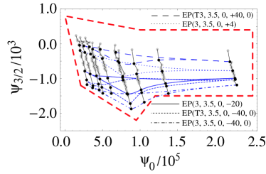
Figure 21: Projection of the E models with nonzero $\tilde{z}_{1}$ into the $(\psi_{0},\psi_{3/2})$ plane (shown in black dots.) The new points sit quite well along the BH mass lines of the 17 models investigated in Secs. VI.2, VI.3 and VI.4. We use the notation EP$(3,3.5,\hat{\theta},\tilde{z}_{1},\tilde{z}_{2})$ and denote by EP(T3, …) the two-body model in which the coefficient $A(r)$ is PN expanded [see Eq. (88)].

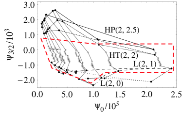
Figure 22: Projections of HT and HP models at 2PN and L models into the $(\psi_{0},\psi_{3/2})$ plane (shown in black dots.) The projections of the previous 17 models are shown in gray dots.

In our construction of the effective template bank, we have been focusing until now on a subset of 17 models. The models we left out are: E models at 3PN with $\tilde{z}_{1,2}$ nonzero, HT and HP models at 2PN, and L models.

As we can see from Fig. 21, E models with $\tilde{z}_{1,2}$ nonzero have a very similar behavior to the 17 models investigated above. Indeed: (i) the projection of the PN waveforms from the same model occupy regions that are triangular, and (ii) the projections of PN waveforms of a given mass lies on the BH mass line spanned by the previous 17 models. In addition, their projections lie roughly in the region we have already defined in Secs. VI.2, VI.3 and VI.4. However, the ending frequencies of these models can be much lower than the values we have set for the detection templates: the detection templates (in all four subregions) should be extended to lower cutoff frequencies if we decide to match these models, up to FF $\sim 0.95$. A rough estimate shows that this increases the number of templates to about twice the original value.

In Fig. 22, we plot the projections of the L$(2,0)$, L$(2,1)$, HT$(2,2)$ and HP$(2,2.5)$ waveforms into the $(\psi_{0},\psi_{3/2})$ plane. As we already know, these models are not matched by the detection templates as well as the other 17 models. Here we can see that their projections onto the $(\psi_{0},\psi_{3/2})$ plane are also quite dissimilar from those models. For L models, although different masses project into a triangular region, the projection of each mass configuration does not align along the corresponding BH mass line generated by the 17 models. In order to cover the $L$ models up to FF$\sim 0.93$, we need to expand the $(\psi_{0},\psi_{3/2})$ region only slightly. However, as we read from Tab. LABEL:tableETB1, the cutoff frequencies need to be extended to even lower values than for the E models with nonzero $\tilde{z}_{1,2}$. Luckily, this expansion will not cost much. In the end the total number of templates needed should be about three times the original value.

For HT and HP models at 2PN, the projections almost lie along the BH mass lines, but the regions occupied by these projections have weird shapes. We have to extend the $(\psi_{0},\psi_{3/2})$ region by a factor $\sim 2$ in order to cover the phasings. [The ending/cutoff frequencies for these models are higher than for the previous two types of models.] An additional subtlety in this case is that, as we can read from Tab. LABEL:tableETB1, the optimal values of $\alpha$ are often negative, since the amplitude becomes higher than the $f^{-7/6}$ power law at higher frequencies. This expansion of the range of $\alpha$ affects both the choice of the discrete cutoff frequencies and the placement of $(\psi_{0},\psi_{3/2})$ lattices. This effect is yet to be estimated.

Finally, we notice that if these extensions are made, then the estimation of the chirp mass from the coefficient $\psi_{0}$ becomes less accurate than the one given in Table 10.

VI.6 Extension of the Fourier-domain detection template family to more than two phasing parameters

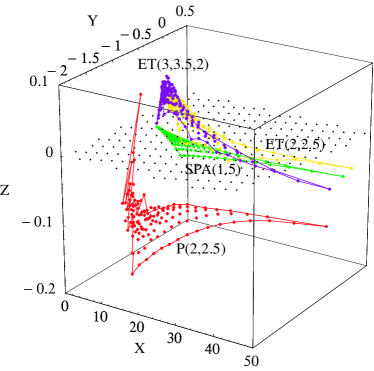
Figure 23: Projection of the models P$(2,2.5)$, ET$(2,2.5)$, ET$(3,3.5,0)$, and SPA(1.5) onto the three-parameter Fourier-domain detection template, for many BBH masses that lie within the same ranges taken in Fig. 20. The variables $(X,Y,Z)$ are related to $(\psi_{0},\psi_{1},\psi_{3/2})$ by a linear transformation, constructed so that the mismatch metric is just $\delta_{ij}$ and that the $(\psi_{0},0,\psi_{3/2})$ plane is mapped to the $(X,Y,0)$ plane. The dots show the value of the parameters $(X,Y,Z)$ where the match with one of the PN waveforms is maximum.

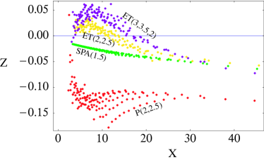
Figure 24: $(X,Z)$ section of Fig. 23. Comparison with Fig. 23 shows that all the projections lie near the $(X,0,Z)$ plane.

It might seem an accident that by using only two phasing parameters, $\psi_{0}$ and $\psi_{3/2}$, we are able to match very precisely the wide variety of PN waveforms that we have considered. Indeed, since the waveforms predicted by each PN model span a two-dimensional manifold (generated by varying the two BH masses $m_{1}$ and $m_{2}$ or equivalently the mass parameters $M$ and $\eta$), we could naturally expect that a third parameter is required to incorporate all the PN models in a more general family, and to add even more signal shapes that extrapolate beyond the phasings and amplitudes seen in the PN models.

In particular, because the accumulation of signal-to-noise ratio is more sensitive to how well we can match the phasing (rather than the amplitude) of PN templates, such a third parameter should probably interpolate between phasings predicted by different PN models. As a consequence, the amplitude parameters $f_{\rm cut}$ and ${\cal A}$ do not generate a real dimensional extension of our detection template family. In this section, we present a qualitative study of the extension of our detection template family obtained by adding one phasing parameter, the parameter $\psi_{1}$ of Eq. (109).

We use the $(\psi_{0},\psi_{1},\psi_{3/2})$ Fourier-domain detection templates to match the PN waveforms from the models P$(2,2.5)$, ET$(2,2.5)$, and ET$(3,3.5,0)$; these models were chosen because their projections onto the $(\psi_{0},\psi_{3/2})$ detection templates were rather distant in the $(\psi_{0},\psi_{3/2})$ parameter space. Throughout this section (and unlike the rest of this paper), we use an approximated search procedure whereby we essentially replace the amplitude of the target models with the Newtonian amplitude ${\cal A}(f)=f^{-7/6}$ with a cutoff frequency $f_{\mathrm{cut}}$ [we always assumed ${\cal A}=0$ and $f_{\rm cut}=400$ Hz]. As expected, the matches increase, and indeed they are almost perfect: always higher than $0.994$ (it should be remembered however that these should be considered as matches of the PN phasings rather than as matches of the PN waveforms; especially for high masses, the frequency dependence of the amplitude is likely to change these values).

If we plot the projections of the PN waveforms in the $(\psi_{0},\psi_{1},\psi_{3/2})$ space, we find that the clusters of points corresponding to each PN target model look quite different from the projections [onto the $(\psi_{0},\psi_{3/2})$ template space] shown in Fig. 20; but this is just an artifact of the parametrization. We can perform a linear transformation $(\psi_{0},\psi_{1},\psi_{3/2})\rightarrow(X,Y,Z)$, defined in such a way that (i) in the $(X,Y,Z)$ parameters, the mismatch metric is just $\delta_{ij}$, and that (ii) the $(\psi_{0},0,\psi_{3/2})$ plane is mapped to the $(X,Y,0)$ plane. These conditions define the linear transformation up to a translation and a rotation along the $Z$ axis; to specify the transformation completely we require also that all the projections of the PN models lie near the origin, and be concentrated around the $X$ axis. Figure 23 shows the projection of the PN models P$(2,2.5)$, ET$(2,2.5)$, and ET$(3,3.5,0)$ onto the $(\psi_{0},\psi_{1},\psi_{3/2})$ detection template family, as parametrized by the $(X,Y,Z)$ coordinate system, for many BBH masses that lie within the same ranges of Fig. 20. Each dot marks the parameters $(X,Y,Z)$ that best match the phasing of one of the PN waveforms. We include also the projection of a further PN model, SPA(1.5), obtained by solving the frequency-domain version of the balance equation, obtained in the stationary-phase approximation from our T model. The expression of the SPA(1.5) phasing as a function of $f$ coincides with our Eq. (109), but the coefficients that correspond to $(\psi_{0},\psi_{1},\psi_{3/2})$ are functions of the two mass parameters $M$ and $\eta$.

By construction, the match between nearby detection templates is related to their Euclidian distance in the $(X,Y,Z)$ by

$$1-{\rm overlap}=\Delta X^{2}+\Delta Y^{2}+\Delta Z^{2}\,.$$ (144)

We see immediately that all the PN models are not very distant from the $(X,Y,0)$ plane [also shown in the figure], which coincides with the $(\psi_{0},\psi_{3/2})$ plane. The farthest model is P$(2,2.5)$, with a maximum distance $\sim 0.18$. It is important to notice that, since this number is obtained by assuming $f_{\rm cut}=400$ Hz and ${\cal A}=0$, it tends to underestimate the true overlaps for models that end below $400$ Hz, such as the P models at higher masses. See also Fig. 24 for an $(X,Z)$ section of Fig. 23.

We can study the relation between this three-dimensional family of templates and the two-dimensional family considered earlier by projecting the points of Fig. 23 onto the $(X,Y,0)$ plane [which corresponds to the $(\psi_{0},0,\psi_{3/2})$ plane]. The resulting images resemble closely the projections of the PN models onto the $(\psi_{0},\psi_{3/2})$ parameter space of the two-dimensional family, as seen in the left panel of Fig. 25. However, the agreement is poor for P$(2,2.5)$ because of the relatively high cut frequency $f_{\rm cut}=400$ Hz. The right panel of Fig. 25 was obtained by taking $f_{\rm cut}=200$ Hz. The agreement is much better. This result goes some way toward explaining why using only two phasing parameters was enough to match most PN models in a satisfactory way.

As stated at the beginning of this section, the parameter $Z$ can indeed be used to expand the dimensionality of our detection template family, because it appears to interpolate between different PN models. It is possible that the number of $Z$ values needed when laying down a discrete template family might not be too large, because the PN models do not seem to lie very far from the $Z=0$ plane [remember that distances in the $(X,Y,Z)$ parameter space are approximately mismatch distances].

The good performance that we find for the two- and three-dimensional Fourier-domain families confirms the results obtained in Refs. DIS3 , CA and EPT . In Ref. DIS3 , the authors point out that the waveforms obtained from the stationary phase approximation at 2PN and 2.5PN order are able to approximate the E models, throughout most of the LIGO band, by maximizing over the mass parameters [see Ref. DIS3 , in particular the discussion of their model “Tf2,” and the discussion around their Fig. 2].

In Ref. CA , Chronopolous and Apostolatos show that what would be in our notation the SPA$(2)$ model (where the phasing is described by a fourth-order polynomial in the variable $f^{1/3}$) can be approximated very well, at least for the purpose of signal detection, by the SPA$(1.5)$ model, with the advantage of having a much lower number of templates. In Ref. EPT , the authors go even further, investigating the possibility of approximating the SPA$(2)$ phasing with a polynomial of third, second and even first degree obtained using Chebyshev approximants.

It is important to underline that in all of these analyses the coefficients that appear in the expression of the phasing [corresponding to our $\psi_{0},\psi_{1},\ldots$ in Eq. (109)] depend on only two BBH mass parameters, either directly DIS3 ; CA , or indirectly EPT through specific PN relations at each PN order. As a consequence, the phasings assumed in these references are confined to a two-dimensional submanifold analog to the surface labeled “SPA$(1.5)$” in Fig. 23.

In this paper we follow a more general approach, because the phasing coefficients $\psi_{i}$ are initially left completely arbitrary. Only after studying systematically the projection of the PN models onto the template bank we have determined the region where a possible detection template bank would be laid down. The high matches that we find between detection templates and the various PN models depend crucially on this assumption. As a consequence, our parameters $\psi_{i}$ do not have a direct physical meaning, and they cannot easily be traced back to specific functions of the BBH masses, except for the chirp mass, as seen in Sec. VI.4. This is natural, because our detection templates are built to interpolate between different PN models, each of which has, as it were, a different idea of what the waveform for a BBH of given masses should be.

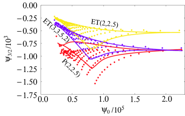
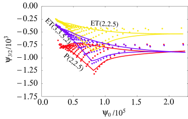
Figure 25: In this figure, we compare the projection of the PN models onto the three-dimensional $(\psi_{0},\psi_{1},\psi_{3/2})$ Fourier-domain detection template family [shown by the dots as a two-dimensional section in the $(\psi_{0},\psi_{3/2})$ submanifold] with the projection of the PN models in the two-dimensional $(\psi_{0},\psi_{3/2})$ template family [shown by the lines]. In the left panel, we use ${\cal A}=0$ and $f_{\rm cut}=400$ Hz to maximize the matches; in the right panel we use ${\cal A}=0$ and $f_{\rm cut}=200$ Hz.

VII Performance of the time-domain detection templates and construction of the detection bank in time domain

Another possibility of building a detection template family is to adopt one or more of the physical models discussed in Secs. IV as the effective template bank used for detection. Under the general hypothesis that underlies this work (that is, that the target models span the region in signal space where the true physical signals reside), if we find that one of the target models matches all the others very well, we can use it as the effective model; and we can estimate its effectualness in matching the true physical signal from its effectualness in matching all the other models.

As shown in Tables IV.2, IV.2 and discussed in Sec. V, the fitting factors FF for the projection of the PN models onto each other are low (at least for PN order $n\leq 2.5$ or for high masses); in other words, the models appear to be quite distant in signal space. This conclusion is overturned, however, if we let the dimensionless mass ratio $\eta$ move beyond its physical range $0\leq\eta\leq 1/4$. For instance, the P$(2,2.5)$ and EP$(3,3.5,0)$ models can be extended formally to the range $0\leq\eta\leq 1$. Beyond those ranges, either the equations (of energy-balance, or motion) become singular, or the determination of the MECO or light ring (the evolutionary endpoint of the inspiral for the P$(2,2.5)$ model and the EP$(3,3.5,0)$ model, respectively) fails.

When the models are extended to $0<\eta\leq 1$, they appear to lie much closer to each other in signal space. In particular, the P$(2,2.5)$ and EP$(3,3.5,0)$ models are able to match all the other models, with minmax $\mathrm{FF}>0.95$, for almost all the masses in our range, and in any case with much improved $\mathrm{FF}$ for most masses; see Tables LABEL:tableXV and LABEL:tableXVI. Apparently, part of the effect of the different resummation and approximation schemes is just to modulate the strength of the PN effects in a way that can be simulated by changing $\eta$ to nonphysical values in any one model. This fact can be appreciated by looking at Figs. 26, 27 and 28, 29, which show the projection of several models onto the P$(2,2.5)$ and EP$(3,3.5,0)$ effective template spaces, respectively. For instance, in comparison with T$(2,2.5)$, the model P$(2,2.5)$ seems to underestimate systematically the effect of $\eta$, so a satisfactory FF for $\eta_{T}=0.25$ can be obtained only if we let $\eta_{P}>0.25$ (quite consistently, in the comparison of Tables IV.2, IV.2, where $\eta$ was confined to its physical range, T$(2,2.5)$ could match P$(2,2.5)$ effectively, but the reverse was not true).

The other (and perhaps crucial) effect of raising $\eta$ is to change the location of the MECO for the P-approximant model (or the light ring, for the EP model), where orbital evolution ends. (Remember that one of the differences between the Padé and the EOB models is that the latter includes a plunge part between the ISCO and the light ring.) More specifically, for P$(2,2.5)$ [EP$(3,3.5,0)$] the position of the MECO [light ring] is pushed to smaller radii as $\eta$ is increased. This effect can increase the FF for target models that have very different ending frequencies from those of P$(2,2.5)$ and EP$(3,3.5)$ at comparable $\eta$’s.

Because for the EP model the frequency at the light ring is already quite high, we cannot simply operate on $\eta$ to improve the match between the EP model and other models that end at much lower frequencies [see the values of minmax matches in Table LABEL:tableXVI]. Thus, we shall enhance the effectualness of EP by adding an arbitrary cut parameter that modifies the radius $r$ (usually the light-ring radius) at which we stop the integration of the Hamilton equations (91)–(94); the effect is to modify the final instantaneous GW frequency of the waveform. This is therefore a time-domain cut, as opposed to the frequency-domain cuts of the frequency-domain effective templates examined in the previous section.

We can then compute the FF by searching over $f_{\mathrm{cut}}$ in addition to $M$ and $\eta$, and we shall correspondingly account for the required number of distinct $f_{\mathrm{cut}}$ when we estimate the number of templates required to give a certain $\mathrm{MM}_{\mathrm{tot}}$. Even so, if we are unsure whether we can model successfully a given source over a certain range of frequencies that falls within LIGO range (as it is the case for the heavy BBHs with MECOs at frequencies $<$ 200 Hz), the correct way to estimate the optimal $\rho$ (and therefore the expected detection rate) is to include only the signal power in the frequency range that we know well.

The best matches shown in Tables LABEL:tableXV and LABEL:tableXVI, and in Figs. 26–29 were obtained by searching over the target model parameter space with the simplicial amoeba algorithm nrc . We found (empirically) that it was expedient to conduct the searches on the parameters $\beta\equiv M\eta^{2/5}$ and $\eta$ rather than on $M$ and $\eta$. This is because iso-match surfaces tend to look like thin ellipses clustered around the best match parameter pair, with principal axes along the $\beta$ and $\eta$ directions. As shown in Table LABEL:tableXV, the values of the maxmax and minmax FFs are very close to each other for the P$(2,2.5)$ model; the same is true for the EP$(3,3.5)$ model (so in Table LABEL:tableXVI we do not show both). For EP$(3,3.5)$, the search over the three parameters $(\beta,\eta,f_{\mathrm{cut}})$ was performed as a refinement step after a first search on $(\beta,\eta)$.

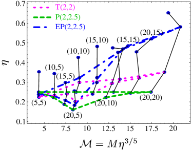
Figure 26: Projection of 2PN waveforms onto the P$(2,2.5)$ effective template space. Dots are shown for the same BBH masses of Tab. LABEL:tableETB1, and for PN models T$(2,2.5)$, P$(2,2.5)$, ET$(2,2.5)$, and EP$(2,2.5)$. The thin solid lines show the BH mass lines (introduced in Sec. VI.2), while the dashed and dotted lines show the contours of the projections of selected PN models.

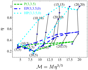
Figure 27: Projection of 3PN waveforms onto the P$(2,2.5)$ effective template space. Dots are shown for the same BBH masses of Tab. LABEL:tableETB1, and for PN models T$(3,3.5,+2)$, P$(3,3.5,+2)$, ET$(3,3.5,+2)$, EP$(3,3.5,+2)$, HT$(3,3.5,+2)$, and HP$(3,3.5,0)$. The dots for $\hat{\theta}=-2$ are only slightly displaced, and they are not shown. The thin solid lines show the BH mass lines (introduced in Sec. VI.2), while the dashed and dotted lines show the contours of the projections of selected PN models.

We have evaluated the mismatch metric O $g_{ij}$ (see Sec. II) with respect to the parameters $(\beta,\eta)$ for the models P$(2,2.5)$ and EP$(3,3.5,0)$ (while evaluating $g_{ij}$, the EP waveforms were not cut). The metric components at the point $(\beta_{0},\eta_{0})$ were obtained by first determining the ranges $(\beta_{\mathrm{min}},\beta_{\mathrm{max}})$, $(\eta_{\mathrm{min}},\eta_{\mathrm{max}})$ for which

$${\langle u(\beta_{0},\eta_{0}),u(\beta_{\mathrm{min}},\eta_{0})\rangle} = {\langle u(\beta_{0},\eta_{0}),u(\beta_{\mathrm{max}},\eta_{0})\rangle}=1-0.05$$ (145)

$${\langle u(\beta_{0},\eta_{0}),u(\beta_{0},\eta_{\mathrm{min}})\rangle} = {\langle u(\beta_{0},\eta_{0}),u(\beta_{0},\eta_{\mathrm{max}})\rangle}=1-0.05;$$ (146)

then a quadratic form was least-squares–fit to 16 values of the match along the ellipse $\Gamma_{1}$ with axes given by $(\beta_{\mathrm{min}},\beta_{\mathrm{max}})$ and $(\eta_{\mathrm{min}},\eta_{\mathrm{max}})$. The first quadratic form was used only to determine the principal axes of two further ellipses $\Gamma_{2}$ and $\Gamma_{3}$, at projected matches of $1-0.025$ and $1-0.0125$. Another quadratic form (giving the final result for the metric) was then fit at the same time to 16 points along $\Gamma_{2}$ and to 16 points along $\Gamma_{3}$, but the two ellipses were given different fitting weights to cancel the quartic correction terms in the Taylor expansion of the match around $(\beta_{0},\eta_{0})$ [the cubic terms were canceled automatically by taking symmetric points along the ellipses]. The rms error of the fit was in all cases very good, establishing that the quadratic approximation held in the close vicinity (matches $\sim 0.95$) of each point.

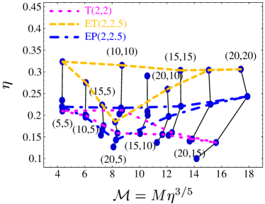
Figure 28: Projection of 2PN waveforms onto the EP$(3,3.5)$ effective template space. This projection includes the effect of the frequency cut. Dots are shown for the same BBH masses of Tab. LABEL:tableETB1, and for PN models T$(2,2.5)$, P$(2,2.5)$, ET$(2,2.5)$, and EP$(2,2.5)$. The thin solid lines show the BH mass lines (introduced in Sec. VI.2), while the dashed and dotted lines show the contours of the projections of selected PN models.

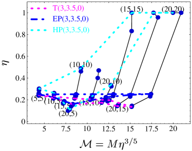
Figure 29: Projection of 3PN waveforms onto the EP$(3,3.5)$ effective template space. This projection includes the effect of the frequency cut. Dots are shown for the same BBH masses of Tab. LABEL:tableETB1, and for PN models T$(3,3.5,+2)$, P$(3,3.5,+2)$, ET$(3,3.5,+2)$, EP$(3,3.5,+2)$, HT$(3,3.5,+2)$, and HP$(3,3.5,+2)$. The dots for $\hat{\theta}=-2$ are only slightly displaced, and they are not shown. The thin solid lines show the BH mass lines (introduced in Sec. VI.2), while the dashed and dotted lines show the contours of the projections of selected PN models.

We estimate that the numerical error $\sim 20\%$ is in any case less than the error associated with using Eq. (25) to evaluate the required number of templates, instead of laying down a lattice of templates more accurately.

The resulting $\sqrt{|g|}$ for P$(2,2.5)$ and EP$(3,3.5,0)$ is shown in Fig. 30. It is evident that most of the mismatch volume is concentrated near the smallest $\beta$’s and $\eta$’s in parameter space. This is encouraging, because it means that the extension of the effective template family to high masses and high $\eta$’s (necessary, as we have seen, to match several target models with very high FF) will be relatively cheap with respect to the size of the template bank (this picture, however, changes when we introduce frequency-domain cuts for the EP models). With the $\sqrt{|g|}$’s we then computed the number of P and EP templates necessary to cover the parameter ranges $\beta:(4,24)$, $\eta:(0.15,1.00)$, and $\beta:(4,24)$, $\eta:(0.1,1.00)$ which span comfortably all the projected images of the target spaces onto the P and EP template spaces, respectively. [Note the ranges include also BBHs where one of the BH has a mass less than $5M_{\odot}$.] We obtained

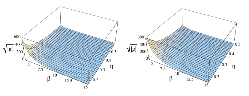
Figure 30: Determinant of the mismatch metric for the P$(2,2.5)$ models [left panel], and for the EP$(3,3.5,0)$ models [right panel]. The determinant $\sqrt{|g|}$ is shown as a function of $\eta$ and $\beta=M\eta^{2/5}$.

$$\mathcal{N}_{P}\simeq 3260\left(\frac{0.02}{1-\mathrm{MM}}\right),\quad\quad\mathcal{N}_{E}\simeq 6700\left(\frac{0.02}{1-\mathrm{MM}}\right),$$ (147)

where MM is the required minimum match (analog to the parameter $\mathrm{MM}_{\psi}$ of the preceding section). By comparison, these numbers are reduced to respectively $1230$ and $3415$ if we restrict $\eta$ to the physical range.

The number $\mathcal{N}_{E}$ does not include the effect of multiple ending frequencies (cuts). We estimate the number of distinct $f_{\mathrm{cut}}$ needed for each $\beta$ by an argument similar to the one used for the Fourier-domain effective templates (see Sec. VI); it turns out that more cuts are required for higher masses. The resulting number of templates is $\mathcal{N}_{Ec}\simeq 51,000$ for $\mathrm{MM}=0.98$, which is comparable to the result for the effective Fourier-domain templates.

If we assume that the distance between the time-domain templates and the target models is representative of the distance to the true physical signal, we can guess that $\mathrm{FF}\gtrsim 0.95$ for P and $\mathrm{FF}\gtrsim 0.97$ for EP with cuts. Under these hypotheses, 6,500 P templates can buy us a (worst-case) $\mathrm{MM}_{\mathrm{T}}\simeq 0.94$, corresponding to a loss in event rate of $\sim 17\%$. For 51,000 EP templates, we get $\mathrm{MM}_{\mathrm{T}}\simeq 0.95$, corresponding to a loss in event rate of $\sim 14\%$.

Before ending this section we would like to point out another time-domain detection-template family which can be consider kindred of the Fourier-domain detection-template family introduced in Sec. VI, see Eq. (107). We can use, for example, the following expression suggested by PN calculations [see, e.g., Ref. BIWW ]

$$h_{\rm eff}(t)={\cal A}^{\rm T}_{\rm eff}(t)\,e^{i\psi^{\rm T}_{\rm eff}(t)}\,,$$ (148)

where

$${\cal A}^{\rm T}_{\rm eff}(t)=(t_{c}-t)^{7/16}\,\left[1-\alpha^{\rm T}\,(t_{c}-t)^{-1/4}\right]\,\theta(t_{\rm cut}-t)\,,$$ (149)

$${\psi}_{\rm eff}(t) = \phi_{c}+(t_{c}-t)^{5/8}\,\left[\psi^{\rm T}_{0}+\psi^{\rm T}_{1/2}\,(t_{c}-t)^{-1/8}+\psi^{\rm T}_{1}\,(t_{c}-t)^{-1/4}\right.$$ (150)

$$\left.+\psi^{\rm T}_{3/2}\,(t_{c}-t)^{-3/8}+\psi^{\rm T}_{2}\,(t_{c}-t)^{-1/2}+\cdots\right]\,,$$

where $\phi_{c},t_{c},\alpha^{\rm T},\psi^{\rm T}_{0},\psi^{\rm T}_{1},\psi^{\rm T}_{3/2}$ and $\psi^{\rm T}_{2}$ are arbitrary parameters whose range of values are determined maximizing the matches with the target two-body models.

VIII Summary

This paper deals with the problem of detecting GWs from the most promising sources for ground-based GW interferometers: comparable-mass BBHs with total mass $M=10\mbox{--}40M_{\odot}$ moving on quasicircular orbits. The detection of these sources poses a delicate problem, because their transition from the adiabatic phase to the plunge, at least in the nonspinning case, is expected to occur in the LIGO and VIRGO frequency bands. Of course, the true GW signals from these inspirals should be obtained from exact solutions of the Einstein equations for two bodies of comparable mass. However, the theoretical templates used to search for these signals will be, at best, finite-order approximations to the exact solutions, usually derived in the PN formalism. Because the perturbative PN approach begins to fail during the final stages of the inspiral, when strong curvature and nonlinear effects can no longer be neglected, various PN resummation methods have been introduced BD1 ; BD2 ; EOB3PN to improve the convergence of the PN series.

In the first part of this paper [see Sec. III,  IV and V] we studied and compared in detail all the PN models of the relativistic two-body dynamics currently available, including PN Taylor-expanded and resummed models both in the adiabatic approximation and in the nonadiabatic case. We noticed the following features [see Tables IV.2, IV.2]. At least for PN orders $n\leq 2.5$, the target models T, P, and E have low cross matches, if the 2.5PN Taylor flux is used. For example, for almost all the masses in our range, we found $\mathrm{maxmax}\,\mathrm{FF}\leq 0.9$; the matches were much better only for P against E (and viceversa). However, if the 2PN Taylor flux is used the overlaps are rather high. At 3PN order we found much higher matches between T, P, and E, and also with the nonadiabatic model H, at least for masses $M\leq 30M_{\odot}$, and restricting to $\tilde{z}_{1}=0=\tilde{z}_{2}$. These results make sense because at 3PN order the various approximations to the binding energy and the flux seem to be much closer to each other than at lower orders. This “closeness” of the different analytical approaches, which at 3PN order are also much closer to some examples of numerical quasiequilibrium BBH models GGB , was recently pointed out in Refs. LB ; DGG . On the other hand, the extraction of BBH parameters from a true measured signal, if done using the 3PN models, would still give a range of rather different estimates. However, we want to point out that for quite high masses, e.g., $M=40M_{\odot}$, the 3PN models can have again lower overlaps, also from the point of view of detection.

In addition, by studying the frequency-domain amplitude of the GW signals that end inside the LIGO frequency band [see Figs. 4, 7, 14, 10], we understood that if high matches are required it is crucial to reproduce their deviations from the Newtonian amplitude evolution, $f^{-7/6}$ (on the contrary, the Newtonian formula seems relatively adequate to model the PN amplitude for GW frequencies below the instantaneous GW frequency at the endpoint of orbital evolution).

Finally, the introduction of the HT, HP and L models in Secs. IV.1, IV.2 provided another example of two-body nonadiabatic dynamics, quite different from the E models. In the H models, the conservative dynamics does not have an ISCO [see the discussion below Eq. (73)] at 2PN and 3PN orders. As a consequence, the transition to the plunge is due to secular radiation-reaction effects, and it is pushed to much higher frequencies. This means that, for the H models, the GW signals for BBHs of total mass $M=10\mbox{--}40M_{\odot}$ end outside the LIGO frequency band, and the frequency-domain amplitude does not deviate much from the Newtonian result, at least until very high frequencies [see Fig. 10]. The L models do not provide the waveforms during the late inspiral and plunge. This is due to the fact that because of the appearance of unphysical effects, e.g., the binding energy starts to increase with time instead of continuing decreasing, we are obliged to stop the evolution before the two BHs enter the last stages of inspiral. It is important to point out that differently from the nonadiabatic E models, the nonadiabatic H and L models give rather different predictions when used at various PN orders. So, from these point of view they are less reliable and robust than the E models.

In the second part of this paper [Secs. VI,  VII] we pursued the following strategy. We assumed that the target models spanned a region in signal space that (almost) included the true GW signal. We were then able to provide a few detection template families (either chosen among the time-domain target models, or built directly from polynomial amplitude and phasings in the frequency domain) that approximate quite well all the targets [$\mathrm{FF}\geq 0.95$ for almost all the masses in our range, with much better $\mathrm{FFs}$ for most masses]. We speculate that the effectualness of the detection model in approximating the targets is indicative of its effectualness in approximating the true signals.

The Fourier-domain detection template family, discussed in Sec. VI, is simple and versatile. It uses a PN polynomial structure for the frequency-domain amplitude and phasing, but it does not constrain the coefficients to the PN functional dependencies on the physical parameters. In this sense this bank follows the basic idea that underlies the Fast Chirp Transform JP . However, because for the masses that we consider the GW signal can end within the LIGO frequency band, we were forced to modify the Newtonian-order formula for the amplitude, introducing a cutoff frequency and a parameter to modify the shape of the amplitude curve (the parameter $\alpha$). As discussed at the end of Sec. VI.6 the good performance of the two and three-dimensional families confirms also results obtained in Refs. DIS3 , CA and EPT .

We showed that our Fourier-domain detection template space has a FF higher than $0.97$ for the T, P and E models, and $\gtrsim 0.96$ for most of the 3PN HT and HP models; we then speculate that it will match true BBH waveforms with FF $\sim 0.96$. We have computed the number of templates required to give MM $\simeq 0.96$ (about $10^{4}$). The total $\mathrm{MM}_{\mathrm{T}}$ should be larger than ${\rm FF}\cdot{\rm MM}\sim 0.92$, which corresponds to a loss of event rate of $1-{\rm MM}_{\mathrm{T}}^{3}\approx 22\%$. This performance could be improved at the price of introducing a larger number of templates, with the rough scaling law of ${\cal N}=10^{4}[0.04/(0.96-{\rm MM})]^{2}$.

In Sec. VI.5 we investigated where the less reliable 2PN H and L models, and the E models at 3PN order further expanded considering $\tilde{z}_{1}\neq 0$, lie in the detection template space. The Fourier-domain template family has FF in the range [0.85,0.95] with the 2PN H models, and FF mostly higher than 0.95, but with several exceptions which can be as low as 0.93 with the L models. The E models with $\tilde{z}_{1}\neq 0$ are matched by the detection template family with FF almost always higher than 0.95. The E models with $\tilde{z}_{1}\neq 0$ and the L models are (almost) covered by the region delimiting the adiabatic models and the E models with $\tilde{z}_{1}=0$. However, these models require lower cutoff frequencies, which will increase the number of templates up to a factor of $3$. The 2PN H models sit outside this region and if we want to include them the number of templates should be doubled.

The time-domain detection template families, discussed in Sec. VII, followed a slightly different philosophy. The idea in this case was to provide a template bank that, for some choices of the parameters, could coincide with one of the approximate two-body models. Quite interestingly, this can be achieved by relaxing the physical hypothesis that $0\leq\eta\leq 0.25$. However, the good performances of these banks are less systematic, and harder to generalize than the performance of the Fourier-domain effective bank. As suggested at the end of Sec. VII [see Eq. (148)], the time-domain bank could be improved by using a parametrization of the time-domain amplitude and phase similar to the one used for the Fourier-domain templates. The detection template families based on the extension of the P$(2,2.5)$ and EP$(3,3.5)$ to nonphysical values of $\eta$ were shown to have FF respectively $\gtrsim 0.95$ and $\gtrsim 0.97$ for all the PN target models, and considerably higher for most models and masses. We have computed the number of P templates needed to obtain a $\mathrm{MM}=0.99$ (about 6,500) and of EP templates to obtain a $\mathrm{MM}=0.98$ (about 51,000). The expected total $\mathrm{MM}_{\mathrm{T}}$ is then respectively $\gtrsim 0.94$ and $\gtrsim 0.95$, corresponding to losses in event rate of $\lesssim 17$% and $\lesssim 14$%. The MMs scale roughly as $[0.01/(1-\mathrm{MM})]$ for P and $[0.02/(1-\mathrm{MM})]^{2}$ for EP (because of the additional frequency-cut parameter).

We notice that the number of templates that we estimate for the Fourier- and time-domain detection template families is higher than the number of templates we would obtain using only one PN model. However, the number of independent shapes that enters the expression for the $\rho_{*}$ threshold [see Eq. 18] does not coincide with the number of templates that are laid down within a discrete template bank to achieve a given MM; indeed, if MM is close to one, these are almost guaranteed to be to yield S/N statistics that are strongly correlated. A rough estimate of the number of independent shapes can be obtained taking a coarse-grained grid in template space. For example by setting MM=0 in Eq. (25), the number of independent shapes would be given roughly by the volume of the template space. As explained at the end of Sec. II.2, if we wish to keep the same false-alarm probability, we have to increase the threshold by $\sim 3\%$ if we increase the number of independent shapes by one order of magnitude. This effect will cause a further loss in event rates BS .

Finally, in Sec. VI.6 we extended the detection template family in the Fourier domain by requiring that it embeds the targets in a signal space of higher dimension (with more parameters). We investigated the three dimensional case and we found, as expected, the maxmax matches increase. In particular, the match of the phasings are nearly perfect: always higher than $0.994$ for the two-body models which are farthest apart in the detection template space. Moreover, by projecting the points in the three-dimensional space back to the two-dimensional space, we can get nearly the same projections we would have got from matching directly the PN waveforms with the two-parameter–phasing model. The analysis done in Sec. VI.6 could suggest ways of systematically expand the Fourier-domain templates. Trying to guess the functional directions in which the true signals might lie with respect to the targets was the most delicate challenge of our investigation. However, our suggestions are not guaranteed to produce templates that will capture the true signal, and they should be considered as indications. When numerical relativity provides the first good examples of waveforms emitted in the last stages of the binary inspiral and plunge, it will be very interesting to investigate whether the matches with our detection template families are high and in which region of the detection template space do they sit.

Table 11: (Continued into Table IV.2.) Fitting factors between several PN models, at 2PN and 3PN orders. For three choices of BBH masses, this table shows the maxmax matches [see Eq. (10)] between the search models at the top of the columns and the target models at the left end of the rows, maximized over the intrinsic parameters of the search models in the columns. For each intersection, the three numbers mm, $M=m_{1}+m_{2}$ and $\eta=m_{1}m_{2}/M^{2}$ denote the maximized match and the search-model mass parameters at which the maximum is attained. In computing these matches, the parameter $\eta$ of the search models was restricted to its physical range $0<\eta\leq 1/4$. The arbitrary flux parameter $\hat{\theta}$ was always set equal to zero. These matches represent the fitting factors [see Eq. (20)] for the projection of the target models onto the search models. The reader will notice that the values shown are not symmetric across the diagonal: for instance, the match for the search model T$(2,2.5)$ against the target model P$(2,2.5)$ is higher than the converse. This is because the matches represent the inner product (1) between two different pairs of model parameters: in the first case, the target parameters $(m_{1}=15M_{\odot},m_{2}=15M_{\odot})_{P}\equiv(M=30M_{\odot},\eta=0.25)_{P}$ are mapped to the maximum-match search parameters $(M=39.7M_{\odot},\eta=0.24)_{T}$; in the second case, the target parameters $(m_{1}=15M_{\odot},m_{2}=15M_{\odot})_{T}\equiv(M=30M_{\odot},\eta=0.25)_{T}$ are mapped to the maximum-match parameters $(M=25.37M_{\odot},\eta=0.24)_{P}$ [so the symmetry of the inner product (1) is reflected by the fact that the search parameters $(M=25.3M_{\odot},\eta=0.24)_{P}$ are mapped into the target parameters $(M=30M_{\odot},\eta=0.25)_{T}$].

Table 12: (Continued from Table IV.2.) Fitting factors between several PN models, at 2PN and 3PN orders. Please see the caption to Table IV.2.

Table 13: Fitting factors between T and ET models, at 2PN and 3PN orders, and for different choices of the arbitrary flux parameter $\hat{\theta}$. For three choices of BBH masses, this table shows the maxmax matches [see Eq. (10)] between the search models at the top of the columns and the target models at the left end of the rows, maximized over the mass parameters of the models in the columns. For each intersection, the three numbers mm, $M$ and $\eta$ denote the maximized match and the search-model mass parameters at which the maximum is attained. The matches can be interpreted as the fitting factors for the projection of the target models onto the search models. See the caption to Table IV.2 for further details.

Table 14: Fitting factors for the projection of EP$(3,3.5,0)$ templates onto themselves, for various choices of the parameters ${z}_{1}$ and ${z}_{2}$. The values quoted are obtained by maximizing the maxmax (mm) match over the mass parameters of the (search) models in the columns, while keeping the mass parameters of the (target) models in the rows fixed to their quoted values, $(15+15)M_{\odot}$, $(15+5)M_{\odot}$ $(5+5)M_{\odot}$. The three numbers shown at each intersection are the maximized match and the search parameters at which the maximum was attained. In labeling rows and columns we use the notation EP$(3,3.5,\hat{\theta},{z}_{1},{z}_{2})$. See the caption to Table IV.2 for further details.

	FF for projection onto the Fourier-domain detection template families
PN model		$f_{\rm end}$	mn	$\psi_{0}$	$\psi_{3/2}$	$\alpha f_{\rm cut}^{2/3}$	$f_{\rm cut}$		$f_{\rm end}$	mn	$\psi_{0}$	$\psi_{3/2}$	$\alpha f_{\rm cut}^{2/3}$	$f_{\rm cut}$
	(20+20)$M_{\odot}$	221.4	0.983	23891.	$-554.63$	$0.949$	240.7	(20+5)$M_{\odot}$	341.2	0.992	77508.	$-1041.30$	$0.897$	347.0
	(20+15)$M_{\odot}$	252.4	0.987	30200.	$-606.41$	$0.975$	272.5	(10+10)$M_{\odot}$	442.8	0.992	72639.	$-768.78$	$0.632$	331.4
T$(2,2)$	(15+15)$M_{\odot}$	295.2	0.989	38126.	$-653.61$	$0.968$	313.5	(15+5)$M_{\odot}$	431.3	0.993	96191.	$-1030.20$	$0.831$	440.8
	(20+10)$M_{\odot}$	291.7	0.989	41735.	$-677.51$	$1.002$	314.2	(10+5)$M_{\odot}$	583.4	0.993	130600.	$-1019.10$	$1.001$	805.3
	(15+10)$M_{\odot}$	352.7	0.991	52565.	$-713.54$	$0.968$	387.1	(5+5)$M_{\odot}$	885.6	0.989	225060.	$-1056.80$	$0.531$	894.4
	(20+20)$M_{\odot}$	161.2	0.970	19807.	$62.32$	$0.691$	224.4	(20+5)$M_{\odot}$	281.6	0.987	71552.	$-188.92$	$0.227$	312.7
	(20+15)$M_{\odot}$	185.9	0.975	25398.	$57.59$	$0.347$	220.3	(10+10)$M_{\odot}$	322.4	0.983	66783.	$-37.92$	$0.490$	630.9
T$(2,2.5)$	(15+15)$M_{\odot}$	214.9	0.979	32787.	$40.11$	$0.210$	245.0	(15+5)$M_{\odot}$	345.6	0.988	89296.	$-166.70$	$0.107$	373.8
	(20+10)$M_{\odot}$	222.3	0.980	36540.	$28.23$	$0.160$	255.5	(10+5)$M_{\odot}$	443.3	0.989	123100.	$-159.28$	$0.379$	746.0
	(15+10)$M_{\odot}$	261.2	0.983	47008.	$2.24$	$0.107$	293.7	(5+5)$M_{\odot}$	643.9	0.994	217090.	$-194.81$	$0.253$	1033.1
	(20+20)$M_{\odot}$	207.9	0.983	25219.	$-575.44$	$1.002$	265.8	(20+5)$M_{\odot}$	276.1	0.986	79630.	$-1095.00$	$0.743$	238.3
	(20+15)$M_{\odot}$	234.5	0.984	31622.	$-623.54$	$1.005$	268.5	(10+10)$M_{\odot}$	415.9	0.988	73738.	$-701.48$	$0.923$	437.8
T$(3,3.5,+2)$	(15+15)$M_{\odot}$	277.2	0.987	38891.	$-612.96$	$0.990$	306.3	(15+5)$M_{\odot}$	362.3	0.990	97371.	$-988.17$	$0.617$	277.0
	(20+10)$M_{\odot}$	259.3	0.986	43944.	$-729.80$	$0.979$	301.6	(10+5)$M_{\odot}$	518.5	0.990	131210.	$-899.96$	$0.642$	392.3
	(15+10)$M_{\odot}$	324.3	0.987	53869.	$-688.38$	$0.865$	315.6	(5+5)$M_{\odot}$	831.7	0.985	224370.	$-826.19$	$0.563$	886.2
	(20+20)$M_{\odot}$	207.9	0.981	24857.	$-603.44$	$0.983$	246.4	(20+5)$M_{\odot}$	276.1	0.987	80359.	$-1188.90$	$0.825$	257.0
	(20+15)$M_{\odot}$	234.5	0.985	31773.	$-681.75$	$0.983$	252.8	(10+10)$M_{\odot}$	415.8	0.988	74637.	$-810.89$	$0.750$	350.3
T$(3,3.5,-2)$	(15+15)$M_{\odot}$	277.2	0.986	39565.	$-707.26$	$0.933$	277.9	(15+5)$M_{\odot}$	362.3	0.989	97861.	$-1070.50$	$0.661$	267.7
	(20+10)$M_{\odot}$	259.3	0.985	44027.	$-787.96$	$0.900$	251.9	(10+5)$M_{\odot}$	518.5	0.988	131840.	$-992.35$	$0.901$	553.3
	(15+10)$M_{\odot}$	324.3	0.988	54194.	$-761.61$	$0.984$	341.1	(5+5)$M_{\odot}$	831.7	0.982	225550.	$-943.65$	$0.577$	916.3
	(20+20)$M_{\odot}$	142.9	0.972	27006.	$-743.88$	$0.991$	208.5	(20+5)$M_{\odot}$	207.8	0.978	81397.	$-1244.40$	$0.698$	192.4
	(20+15)$M_{\odot}$	162.5	0.977	33307.	$-778.72$	$0.987$	206.7	(10+10)$M_{\odot}$	285.9	0.985	73970.	$-743.09$	$0.681$	245.7
P$(2,2.5)$	(15+15)$M_{\odot}$	190.6	0.980	40486.	$-752.07$	$0.991$	237.0	(15+5)$M_{\odot}$	267.5	0.984	98390.	$-1074.60$	$0.709$	231.8
	(20+10)$M_{\odot}$	185.0	0.977	45403.	$-864.50$	$1.116$	288.3	(10+5)$M_{\odot}$	370.0	0.985	131920.	$-961.15$	$0.758$	346.4
	(15+10)$M_{\odot}$	226.3	0.981	54709.	$-771.73$	$0.867$	232.9	(5+5)$M_{\odot}$	571.8	0.983	224810.	$-867.58$	$0.813$	764.5
	(20+20)$M_{\odot}$	216.4	0.984	24922.	$-523.74$	$0.995$	265.2	(20+5)$M_{\odot}$	265.0	0.985	79624.	$-1070.20$	$0.830$	258.4
	(20+15)$M_{\odot}$	243.6	0.985	31204.	$-564.86$	$1.007$	299.3	(10+10)$M_{\odot}$	432.8	0.990	72663.	$-617.31$	$0.896$	488.2
P$(3,3.5,+2)$	(15+15)$M_{\odot}$	288.5	0.987	38194.	$-541.27$	$0.971$	328.2	(15+5)$M_{\odot}$	359.2	0.990	96933.	$-935.65$	$0.619$	279.6
	(20+10)$M_{\odot}$	265.7	0.986	43280.	$-660.41$	$1.001$	328.8	(10+5)$M_{\odot}$	531.3	0.991	130310.	$-827.00$	$0.843$	588.6
	(15+10)$M_{\odot}$	336.2	0.987	52941.	$-605.52$	$0.902$	356.7	(5+5)$M_{\odot}$	865.6	0.988	223830.	$-780.35$	$0.537$	896.7
	(20+20)$M_{\odot}$	216.4	0.984	24830.	$-545.66$	$1.062$	291.4	(20+5)$M_{\odot}$	265.0	0.986	79956.	$-1114.80$	$0.831$	259.7
	(20+15)$M_{\odot}$	243.6	0.984	31086.	$-583.34$	$0.988$	269.5	(10+10)$M_{\odot}$	432.8	0.990	73167.	$-674.59$	$0.760$	390.9
P$(3,3.5,-2)$	(15+15)$M_{\odot}$	288.5	0.988	38426.	$-581.05$	$0.994$	326.6	(15+5)$M_{\odot}$	359.2	0.990	96850.	$-958.04$	$0.662$	277.7
	(20+10)$M_{\odot}$	265.7	0.986	43464.	$-696.77$	$1.006$	311.2	(10+5)$M_{\odot}$	531.3	0.990	130780.	$-881.70$	$0.810$	539.0
	(15+10)$M_{\odot}$	336.2	0.987	53475.	$-663.65$	$0.882$	333.4	(5+5)$M_{\odot}$	865.6	0.987	224210.	$-828.64$	$0.538$	896.0

& (20+20)$M_{\odot}$ 231.0 0.991 22372. $-258.47$ $0.935$ 477.8 (20+5)$M_{\odot}$ 359.4 0.995 79070. $-857.02$ $0.748$ 519.2 (20+15)$M_{\odot}$ 263.5 0.992 28710. $-302.99$ $0.770$ 425.5 (10+10)$M_{\odot}$ 462.0 0.995 71411. $-420.76$ $0.668$ 722.3 ET$(2,2.5)$(15+15)$M_{\odot}$ 308.0 0.993 36351. $-321.50$ $0.717$ 512.3 (15+5)$M_{\odot}$ 452.7 0.994 96788. $-755.70$ $0.718$ 706.8 (20+10)$M_{\odot}$ 305.1 0.993 41308. $-423.25$ $0.756$ 473.1 (10+5)$M_{\odot}$ 610.1 0.993 129130. $-607.98$ $0.665$ 910.1 (15+10)$M_{\odot}$ 368.3 0.995 51338. $-393.70$ $0.769$ 764.8 (5+5)$M_{\odot}$ 924.0 0.991 221910. $-534.76$ $0.424$ 920.4

(20+20)$M_{\odot}$ 212.1 0.990 22048. $-356.02$ $0.997$ 367.7 (20+5)$M_{\odot}$ 351.3 0.992 78355. $-1057.40$ $0.763$ 402.3 (20+15)$M_{\odot}$ 245.1 0.992 28516. $-423.30$ $0.971$ 415.7 (10+10)$M_{\odot}$ 428.8 0.994 72187. $-631.44$ $0.707$ 616.2 ET$(3,3.5,+2)$(15+15)$M_{\odot}$ 285.8 0.992 36119. $-450.40$ $0.775$ 408.3 (15+5)$M_{\odot}$ 433.7 0.994 96772. $-982.67$ $0.757$ 572.4 (20+10)$M_{\odot}$ 286.6 0.993 40717. $-545.11$ $0.790$ 376.5 (10+5)$M_{\odot}$ 573.1 0.995 130830. $-899.77$ $0.686$ 856.6 (15+10)$M_{\odot}$ 344.5 0.993 51507. $-563.26$ $0.785$ 515.2 (5+5)$M_{\odot}$ 847.9 0.986 225490. $-892.59$ $0.552$ 914.8

(20+20)$M_{\odot}$ 207.1 0.990 21818. $-386.23$ $0.848$ 300.4 (20+5)$M_{\odot}$ 345.9 0.991 78349. $-1103.70$ $0.692$ 379.0 (20+15)$M_{\odot}$ 238.2 0.992 28247. $-451.93$ $0.884$ 347.0 (10+10)$M_{\odot}$ 411.0 0.994 72645. $-709.64$ $0.685$ 499.9 ET$(3,3.5,-2)$(15+15)$M_{\odot}$ 274.0 0.992 36218. $-502.72$ $0.903$ 452.4 (15+5)$M_{\odot}$ 424.8 0.993 97086. $-1052.50$ $0.846$ 600.5 (20+10)$M_{\odot}$ 277.0 0.992 41148. $-613.88$ $0.786$ 364.2 (10+5)$M_{\odot}$ 556.9 0.995 131730. $-1003.30$ $0.699$ 821.5 (15+10)$M_{\odot}$ 330.6 0.992 51702. $-623.17$ $0.822$ 501.2 (5+5)$M_{\odot}$ 816.8 0.983 226430. $-999.02$ $0.539$ 900.4

(20+20)$M_{\odot}$ 218.1 0.991 21315. $-353.42$ $0.773$ 376.1 (20+5)$M_{\odot}$ 345.8 0.990 79526. $-1167.70$ $0.709$ 366.2 (20+15)$M_{\odot}$ 249.1 0.991 28013. $-437.59$ $0.746$ 380.6 (10+10)$M_{\odot}$ 436.2 0.994 73183. $-729.74$ $0.714$ 645.1 EP$(2,2.5)$(15+15)$M_{\odot}$ 290.8 0.991 35947. $-486.80$ $0.672$ 432.2 (15+5)$M_{\odot}$ 433.1 0.994 98170. $-1099.60$ $0.630$ 460.4 (20+10)$M_{\odot}$ 289.8 0.990 40730. $-593.65$ $0.656$ 391.0 (10+5)$M_{\odot}$ 579.6 0.993 132250. $-1014.20$ $0.691$ 868.7 (15+10)$M_{\odot}$ 348.5 0.991 51920. $-632.99$ $0.637$ 451.6 (5+5)$M_{\odot}$ 872.5 0.979 226910. $-997.82$ $0.571$ 833.0

(20+20)$M_{\odot}$ 219.7 0.990 22025. $-329.13$ $0.967$ 398.3 (20+5)$M_{\odot}$ 354.0 0.993 78344. $-1027.30$ $0.668$ 376.6 (20+15)$M_{\odot}$ 251.9 0.991 27970. $-368.53$ $0.888$ 386.4 (10+10)$M_{\odot}$ 439.6 0.994 71704. $-579.45$ $0.719$ 658.8 EP$(3,3.5,+2)$(15+15)$M_{\odot}$ 293.1 0.991 35861. $-409.25$ $0.813$ 452.7 (15+5)$M_{\odot}$ 444.9 0.995 96416. $-934.82$ $0.773$ 608.4 (20+10)$M_{\odot}$ 291.4 0.993 40598. $-512.88$ $0.820$ 429.6 (10+5)$M_{\odot}$ 582.5 0.995 130480. $-855.36$ $0.685$ 879.7 (15+10)$M_{\odot}$ 353.7 0.993 51343. $-527.79$ $0.731$ 495.5 (5+5)$M_{\odot}$ 874.7 0.989 224370. $-820.10$ $0.488$ 916.2

(20+20)$M_{\odot}$ 214.4 0.990 22029. $-349.92$ $0.986$ 384.7 (20+5)$M_{\odot}$ 353.0 0.992 78099. $-1035.10$ $0.692$ 400.3 (20+15)$M_{\odot}$ 248.3 0.992 28185. $-400.30$ $0.849$ 361.2 (10+10)$M_{\odot}$ 430.5 0.994 71820. $-613.97$ $0.718$ 642.1 EP$(3,3.5,-2)$(15+15)$M_{\odot}$ 287.0 0.992 35793. $-429.31$ $0.880$ 510.6 (15+5)$M_{\odot}$ 439.1 0.994 96411. $-960.71$ $0.770$ 591.0 (20+10)$M_{\odot}$ 289.1 0.993 40653. $-537.88$ $0.869$ 452.9 (10+5)$M_{\odot}$ 575.7 0.995 130760. $-899.02$ $0.696$ 877.1 (15+10)$M_{\odot}$ 347.3 0.993 51423. $-558.41$ $0.779$ 494.7 (5+5)$M_{\odot}$ 864.9 0.988 225110. $-886.01$ $0.501$ 909.7

(20+20)$M_{\odot}$ 318.1 0.989 20061. $-192.06$ $0.509$ 379.7 (20+5)$M_{\odot}$ 457.4 0.987 76939. $-936.06$ $0.683$ 450.0 (20+15)$M_{\odot}$ 364.6 0.988 26379. $-249.89$ $0.437$ 385.7 (10+10)$M_{\odot}$ 647.2 0.990 70495. $-502.74$ $0.585$ 666.7 EP$(3,3.5,0,4,0)$(15+15)$M_{\odot}$ 432.0 0.987 34134. $-293.98$ $0.321$ 422.8 (15+5)$M_{\odot}$ 600.6 0.992 95378. $-866.93$ $0.651$ 601.3 (20+10)$M_{\odot}$ 420.4 0.987 38610. $-385.18$ $0.455$ 446.0 (10+5)$M_{\odot}$ 831.6 0.995 129410. $-792.01$ $0.680$ 798.8 (15+10)$M_{\odot}$ 510.8 0.988 49757. $-426.26$ $0.515$ 493.4 (5+5)$M_{\odot}$ 1292.2 0.992 223410. $-772.85$ $0.339$ 1003.8

(20+20)$M_{\odot}$ 118.9 0.970 26410. $-787.54$ $0.964$ 189.8 (20+5)$M_{\odot}$ 215.1 0.989 83591. $-1452.50$ $1.087$ 364.1 (20+15)$M_{\odot}$ 136.9 0.983 33451. $-868.80$ $1.010$ 238.9 (10+10)$M_{\odot}$ 237.8 0.983 76684. $-970.56$ $1.074$ 373.8 EP$(3,3.5,0,-20,0)$(15+15)$M_{\odot}$ 158.5 0.983 41909. $-921.14$ $1.045$ 285.0 (15+5)$M_{\odot}$ 258.0 0.984 101440. $-1323.20$ $1.158$ 486.7 (20+10)$M_{\odot}$ 164.2 0.985 46550. $-1016.40$ $1.138$ 321.2 (10+5)$M_{\odot}$ 327.9 0.977 134130. $-1142.10$ $1.157$ 589.3 (15+10)$M_{\odot}$ 192.4 0.985 56925. $-986.07$ $1.096$ 339.8 (5+5)$M_{\odot}$ 476.1 0.969 226450. $-992.89$ $1.167$ 844.2

(20+20)$M_{\odot}$ 94.0 0.947 29400. $-1174.60$ $1.097$ 184.5 (20+5)$M_{\odot}$ 174.0 0.972 88302. $-1874.90$ $1.073$ 337.6 (20+15)$M_{\odot}$ 108.2 0.962 36837. $-1268.40$ $0.960$ 169.2 (10+10)$M_{\odot}$ 188.0 0.959 82469. $-1437.30$ $1.059$ 411.8 EP$(3,3.5,0,-40,0)$(15+15)$M_{\odot}$ 125.3 0.969 45552. $-1324.90$ $1.010$ 228.4 (15+5)$M_{\odot}$ 206.7 0.967 105660. $-1681.70$ $1.357$ 468.5 (20+10)$M_{\odot}$ 130.4 0.970 50375. $-1423.70$ $1.048$ 252.8 (10+5)$M_{\odot}$ 260.8 0.957 137720. $-1431.90$ $1.111$ 537.6 (15+10)$M_{\odot}$ 152.5 0.964 61789. $-1428.90$ $1.077$ 338.4 (5+5)$M_{\odot}$ 376.1 0.955 228960. $-1185.20$ $1.122$ 874.4

(20+20)$M_{\odot}$ 349.5 0.986 19559. $-43.77$ $0.483$ 374.1 (20+5)$M_{\odot}$ 561.5 0.981 72281. $-542.92$ $0.533$ 549.7 (20+15)$M_{\odot}$ 399.4 0.989 25098. $-58.70$ $0.387$ 384.9 (10+10)$M_{\odot}$ 699.0 0.988 67699. $-246.28$ $0.166$ 463.5 EP$(T_{3},3.5,0,+40,0)$(15+15)$M_{\odot}$ 465.3 0.987 32573. $-86.76$ $0.155$ 341.5 (15+5)$M_{\odot}$ 704.9 0.963 92003. $-570.09$ $1.128$ 522.3 (20+10)$M_{\odot}$ 468.3 0.989 36812. $-153.63$ $0.243$ 430.2 (10+5)$M_{\odot}$ 935.2 0.989 124940. $-469.29$ $0.458$ 787.7 (15+10)$M_{\odot}$ 558.6 0.989 47015. $-159.41$ $0.316$ 652.3 (5+5)$M_{\odot}$ 1398.0 0.989 219670. $-517.04$ $0.986$ 928.5

(20+20)$M_{\odot}$ 95.0 0.953 28875. $-1038.40$ $0.998$ 168.8 (20+5)$M_{\odot}$ 175.2 0.973 87007. $-1721.30$ $1.072$ 348.7 (20+15)$M_{\odot}$ 109.5 0.968 37319. $-1203.50$ $1.186$ 244.7 (10+10)$M_{\odot}$ 190.3 0.975 77432. $-1045.60$ $0.648$ 192.8 EP$(T_{3},3.5,0,-40,0)$(15+15)$M_{\odot}$ 126.9 0.949 44601. $-1160.40$ $1.069$ 322.3 (15+5)$M_{\odot}$ 208.4 0.975 102210. $-1406.10$ $0.805$ 214.6 (20+10)$M_{\odot}$ 131.9 0.978 49188. $-1252.90$ $0.999$ 207.7 (10+5)$M_{\odot}$ 263.3 0.969 135110. $-1218.00$ $1.231$ 548.3 (15+10)$M_{\odot}$ 154.1 0.952 60648. $-1255.90$ $1.017$ 404.3 (5+5)$M_{\odot}$ 380.3 0.965 226990. $-1027.60$ $0.960$ 883.4

(20+20)$M_{\odot}$ 87.0 0.937 18859. $-726.78$ $0.997$ 175.1 (20+5)$M_{\odot}$ 148.9 0.987 72221. $-1938.50$ $0.970$ 209.6 (20+15)$M_{\odot}$ 99.7 0.953 26088. $-939.25$ $1.005$ 175.0 (10+10)$M_{\odot}$ 174.0 0.990 67126. $-1420.30$ $0.986$ 252.5 L(2, 0)(15+15)$M_{\odot}$ 116.0 0.972 34155. $-1087.60$ $0.999$ 189.8 (15+5)$M_{\odot}$ 181.6 0.991 89333. $-1908.10$ $0.996$ 259.5 (20+10)$M_{\odot}$ 118.0 0.974 38075. $-1201.00$ $0.990$ 191.1 (10+5)$M_{\odot}$ 235.9 0.991 120130. $-1869.90$ $0.830$ 274.6 (15+10)$M_{\odot}$ 140.0 0.985 48463. $-1295.00$ $0.996$ 219.6 (5+5)$M_{\odot}$ 348.0 0.994 207730. $-2077.90$ $0.709$ 379.0

(20+20)$M_{\odot}$ 80.3 0.935 33179. $-1379.20$ $0.998$ 136.5 (20+5)$M_{\odot}$ 140.1 0.968 99046. $-2345.10$ $0.996$ 191.6 (20+15)$M_{\odot}$ 92.1 0.960 41065. $-1465.70$ $0.997$ 152.3 (10+10)$M_{\odot}$ 160.5 0.969 85317. $-1293.90$ $0.707$ 167.5 L(2, 1)(15+15)$M_{\odot}$ 107.0 0.969 50159. $-1486.50$ $1.003$ 164.3 (15+5)$M_{\odot}$ 169.6 0.966 114410. $-1835.70$ $0.673$ 165.1 (20+10)$M_{\odot}$ 109.4 0.970 55990. $-1663.30$ $0.994$ 166.4 (10+5)$M_{\odot}$ 218.8 0.964 146040. $-1373.00$ $0.402$ 194.6 (15+10)$M_{\odot}$ 129.4 0.969 66431. $-1519.40$ $0.998$ 187.9 (5+5)$M_{\odot}$ 321.0 0.932 244970. $-1159.90$ $0.743$ 404.3

(20+20)$M_{\odot}$ 389.2 0.964 6138. $1091.40$ $-0.539$ 242.5 (20+5)$M_{\odot}$ 733.9 0.928 31397. $1977.90$ $-0.634$ 981.8 (20+15)$M_{\odot}$ 451.2 0.937 10015. $1120.00$ $0.583$ 693.5 (10+10)$M_{\odot}$ 758.8 0.868 34673. $1301.30$ $0.951$ 783.1 HT$(2,2)$(15+15)$M_{\odot}$ 507.1 0.961 12166. $1236.10$ $-1.842$ 322.1 (15+5)$M_{\odot}$ 849.2 0.905 41087. $1898.60$ $-2.966$ 1192.5 (20+10)$M_{\odot}$ 536.2 0.960 13624. $1378.00$ $-0.711$ 334.7 (10+5)$M_{\odot}$ 1057.3 0.870 109640. $351.04$ $0.939$ 899.7 (15+10)$M_{\odot}$ 632.6 0.950 16662. $1468.50$ $-1.780$ 378.9 (5+5)$M_{\odot}$ 1525.5 0.937 214890. $-317.77$ $0.967$ 969.4

(20+20)$M_{\odot}$ 403.9 0.923 2544. $1511.00$ $0.547$ 459.7 (20+5)$M_{\odot}$ 611.2 0.918 22867. $2595.60$ $-1.053$ 1200.0 (20+15)$M_{\odot}$ 459.0 0.961 1774. $1747.20$ $-1.790$ 279.7 (10+10)$M_{\odot}$ 816.6 0.901 10216. $2343.10$ $-1.861$ 509.6 HP$(2,2.5)$(15+15)$M_{\odot}$ 536.6 0.921 3321. $1853.80$ $0.063$ 1155.9 (15+5)$M_{\odot}$ 771.6 0.892 27498. $2640.30$ $-2.977$ 1200.0 (20+10)$M_{\odot}$ 530.3 0.958 6259. $1961.60$ $-1.844$ 331.6 (10+5)$M_{\odot}$ 1050.2 0.850 107210. $707.41$ $0.893$ 918.8 (15+10)$M_{\odot}$ 638.8 0.914 7474. $2079.90$ $-1.449$ 1193.8 (5+5)$M_{\odot}$ 1601.2 0.921 212810. $33.93$ $0.694$ 916.8

(20+20)$M_{\odot}$ 358.4 0.977 16787. $81.92$ $0.187$ 346.4 (20+5)$M_{\odot}$ 196.3 0.983 83529. $-1429.20$ $0.856$ 232.3 (20+15)$M_{\odot}$ 420.3 0.975 22751. $13.30$ $0.414$ 728.7 (10+10)$M_{\odot}$ 726.0 0.964 67085. $-285.69$ $0.594$ 922.2 HT$(3,3.5,+2)$(15+15)$M_{\odot}$ 484.0 0.971 29634. $8.43$ $0.016$ 417.1 (15+5)$M_{\odot}$ 303.3 0.992 98845. $-1096.60$ $0.782$ 395.9 (20+10)$M_{\odot}$ 495.8 0.983 37522. $-309.28$ $0.693$ 731.8 (10+5)$M_{\odot}$ 970.3 0.992 128810. $-755.33$ $0.526$ 909.7 (15+10)$M_{\odot}$ 586.9 0.967 46435. $-210.60$ $0.586$ 916.7 (5+5)$M_{\odot}$ 1433.6 0.992 221940. $-679.22$ $0.400$ 907.7

(20+20)$M_{\odot}$ 316.4 0.981 17922. $-37.78$ $0.640$ 498.6 (20+5)$M_{\odot}$ 196.1 0.984 83861. $-1489.90$ $0.869$ 232.7 (20+15)$M_{\odot}$ 375.2 0.980 23737. $-95.75$ $0.603$ 618.2 (10+10)$M_{\odot}$ 639.4 0.972 68270. $-408.04$ $0.640$ 917.6 HT$(3,3.5,-2)$(15+15)$M_{\odot}$ 426.3 0.975 31166. $-123.77$ $0.506$ 587.6 (15+5)$M_{\odot}$ 303.1 0.993 98715. $-1142.80$ $0.802$ 389.2 (20+10)$M_{\odot}$ 436.0 0.986 38125. $-390.93$ $0.538$ 434.1 (10+5)$M_{\odot}$ 868.1 0.992 129460. $-848.59$ $0.675$ 852.1 (15+10)$M_{\odot}$ 514.5 0.974 47366. $-316.76$ $0.654$ 806.4 (5+5)$M_{\odot}$ 1273.2 0.993 223420. $-812.58$ $0.425$ 883.0

(20+20)$M_{\odot}$ 474.6 0.968 14652. $236.51$ $0.215$ 863.4 (20+5)$M_{\odot}$ 196.4 0.982 83872. $-1421.20$ $0.928$ 261.4 (20+15)$M_{\odot}$ 539.6 0.966 20205. $181.76$ $0.071$ 1076.9 (10+10)$M_{\odot}$ 952.2 0.948 66050. $-202.66$ $0.548$ 898.9 HP$(3,3.5,+2)$(15+15)$M_{\odot}$ 634.8 0.955 27087. $170.17$ $0.009$ 1200.0 (15+5)$M_{\odot}$ 304.1 0.990 98220. $-1035.20$ $0.796$ 405.4 (20+10)$M_{\odot}$ 598.9 0.975 36238. $-213.15$ $0.438$ 900.5 (10+5)$M_{\odot}$ 1212.8 0.991 127870. $-682.01$ $0.555$ 621.0 (15+10)$M_{\odot}$ 752.5 0.948 45078. $-109.24$ $0.539$ 911.2 (5+5)$M_{\odot}$ 1921.0 0.989 220910. $-608.88$ $0.313$ 925.7

(20+20)$M_{\odot}$ 363.2 0.973 16421. $113.38$ $0.384$ 525.9 (20+5)$M_{\odot}$ 196.3 0.983 83747. $-1435.60$ $0.996$ 289.7 (20+15)$M_{\odot}$ 421.8 0.972 21952. $62.83$ $0.337$ 690.9 (10+10)$M_{\odot}$ 734.7 0.958 66819. $-271.94$ $0.680$ 893.8 HP$(3,3.5,-2)$(15+15)$M_{\odot}$ 489.8 0.968 28632. $62.71$ $0.000$ 422.7 (15+5)$M_{\odot}$ 303.7 0.992 98202. $-1060.60$ $0.749$ 368.8 (20+10)$M_{\odot}$ 510.0 0.982 36893. $-272.30$ $0.263$ 463.2 (10+5)$M_{\odot}$ 998.3 0.991 128060. $-722.63$ $0.491$ 887.7 (15+10)$M_{\odot}$ 591.3 0.959 45653. $-168.47$ $0.469$ 924.6 (5+5)$M_{\odot}$ 1445.9 0.991 221850. $-685.53$ $0.390$ 930.8

	FF for projection onto P$(2,2.5)$, for $0<\eta<1$
		mm	$M$	$\eta$	mn	$M$	$\eta$		mm	$M$	$\eta$	mn	$M$	$\eta$
	(20+20)$M_{\odot}$	$0.997$	$35.53$	$0.35$	$0.994$	$35.55$	$0.35$	(20+5)$M_{\odot}$	$0.988$	$22.04$	$0.21$	$0.979$	$22.51$	$0.20$
	(20+15)$M_{\odot}$	$0.997$	$32.43$	$0.31$	$0.994$	$31.69$	$0.32$	(10+10)$M_{\odot}$	$0.996$	$19.29$	$0.28$	$0.990$	$18.74$	$0.30$
T(2, 2)	(15+15)$M_{\odot}$	$0.997$	$28.45$	$0.29$	$0.993$	$27.54$	$0.32$	(15+5)$M_{\odot}$	$0.993$	$18.31$	$0.23$	$0.985$	$17.94$	$0.24$
	(20+10)$M_{\odot}$	$0.996$	$27.72$	$0.27$	$0.992$	$26.83$	$0.30$	(10+5)$M_{\odot}$	$0.992$	$14.55$	$0.24$	$0.989$	$14.86$	$0.23$
	(15+10)$M_{\odot}$	$0.995$	$23.68$	$0.28$	$0.988$	$22.95$	$0.30$	(5+5)$M_{\odot}$	$0.994$	$10.60$	$0.23$	$0.992$	$10.73$	$0.22$
	(20+20)$M_{\odot}$	$0.821$	$18.77$	$0.94$	$0.962$	$22.59$	$0.65$	(20+5)$M_{\odot}$	$0.958$	$11.66$	$0.63$	$0.987$	$12.81$	$0.53$
	(20+15)$M_{\odot}$	$0.862$	$16.60$	$0.94$	$0.966$	$19.40$	$0.68$	(10+10)$M_{\odot}$	$0.948$	$9.96$	$0.89$	$0.984$	$10.71$	$0.77$
T(2, 2.5)	(15+15)$M_{\odot}$	$0.891$	$14.26$	$0.97$	$0.969$	$16.61$	$0.71$	(15+5)$M_{\odot}$	$0.965$	$9.72$	$0.69$	$0.989$	$10.26$	$0.62$
	(20+10)$M_{\odot}$	$0.905$	$13.67$	$0.94$	$0.974$	$15.95$	$0.69$	(10+5)$M_{\odot}$	$0.971$	$8.58$	$0.60$	$0.987$	$8.67$	$0.59$
	(15+10)$M_{\odot}$	$0.929$	$11.89$	$0.93$	$0.978$	$13.43$	$0.73$	(5+5)$M_{\odot}$	$0.981$	$6.55$	$0.52$	$0.985$	$6.52$	$0.53$
	(20+20)$M_{\odot}$	$0.997$	$37.04$	$0.31$	$0.994$	$36.96$	$0.31$	(20+5)$M_{\odot}$	$0.996$	$23.66$	$0.18$	$0.990$	$23.28$	$0.19$
	(20+15)$M_{\odot}$	$0.997$	$32.62$	$0.29$	$0.995$	$32.69$	$0.29$	(10+10)$M_{\odot}$	$0.998$	$19.70$	$0.26$	$0.993$	$19.24$	$0.27$
T(3, 3.5, 0)	(15+15)$M_{\odot}$	$0.998$	$28.89$	$0.28$	$0.994$	$28.07$	$0.30$	(15+5)$M_{\odot}$	$0.997$	$19.18$	$0.21$	$0.993$	$18.82$	$0.21$
	(20+10)$M_{\odot}$	$0.997$	$28.69$	$0.25$	$0.995$	$28.00$	$0.26$	(10+5)$M_{\odot}$	$0.997$	$14.89$	$0.23$	$0.993$	$14.67$	$0.23$
	(15+10)$M_{\odot}$	$0.998$	$24.35$	$0.26$	$0.994$	$23.72$	$0.27$	(5+5)$M_{\odot}$	$0.999$	$10.16$	$0.24$	$0.997$	$10.27$	$0.24$
	(20+20)$M_{\odot}$	$0.999$	$36.20$	$0.31$	$0.995$	$35.37$	$0.33$	(20+5)$M_{\odot}$	$0.997$	$22.95$	$0.19$	$0.993$	$22.53$	$0.20$
	(20+15)$M_{\odot}$	$0.999$	$31.40$	$0.31$	$0.997$	$31.22$	$0.31$	(10+10)$M_{\odot}$	$0.999$	$18.67$	$0.29$	$0.995$	$18.20$	$0.30$
T(3, 3.5, 0)	(15+15)$M_{\odot}$	$0.999$	$27.63$	$0.29$	$0.997$	$26.96$	$0.31$	(15+5)$M_{\odot}$	$0.997$	$18.61$	$0.22$	$0.995$	$18.15$	$0.23$
	(20+10)$M_{\odot}$	$0.999$	$27.42$	$0.27$	$0.996$	$26.84$	$0.28$	(10+5)$M_{\odot}$	$0.998$	$14.13$	$0.25$	$0.994$	$13.87$	$0.26$
	(15+10)$M_{\odot}$	$0.998$	$23.20$	$0.28$	$0.996$	$22.60$	$0.29$	(5+5)$M_{\odot}$	$0.998$	$9.57$	$0.27$	$0.996$	$9.71$	$0.26$
	(20+20)$M_{\odot}$	$0.998$	$35.30$	$0.33$	$0.996$	$34.73$	$0.34$	(20+5)$M_{\odot}$	$0.998$	$23.03$	$0.19$	$0.995$	$22.62$	$0.20$
	(20+15)$M_{\odot}$	$0.999$	$30.84$	$0.32$	$0.996$	$30.65$	$0.32$	(10+10)$M_{\odot}$	$0.998$	$18.11$	$0.31$	$0.994$	$17.86$	$0.31$
P(3, 3.5, $-2$)	(15+15)$M_{\odot}$	$0.999$	$27.01$	$0.31$	$0.996$	$26.38$	$0.33$	(15+5)$M_{\odot}$	$0.997$	$18.43$	$0.22$	$0.994$	$17.96$	$0.23$
	(20+10)$M_{\odot}$	$0.999$	$26.90$	$0.28$	$0.996$	$26.48$	$0.29$	(10+5)$M_{\odot}$	$0.998$	$13.99$	$0.25$	$0.993$	$13.75$	$0.26$
	(15+10)$M_{\odot}$	$0.998$	$22.76$	$0.29$	$0.995$	$22.18$	$0.31$	(5+5)$M_{\odot}$	$0.997$	$9.50$	$0.27$	$0.996$	$9.63$	$0.27$
	(20+20)$M_{\odot}$	$0.999$	$33.58$	$0.36$	$0.996$	$33.42$	$0.37$	(20+5)$M_{\odot}$	$0.998$	$22.71$	$0.19$	$0.996$	$22.42$	$0.20$
	(20+15)$M_{\odot}$	$0.999$	$30.03$	$0.33$	$0.997$	$29.70$	$0.34$	(10+10)$M_{\odot}$	$0.999$	$17.87$	$0.31$	$0.995$	$17.36$	$0.33$
P(3, 3.5, +2)	(15+15)$M_{\odot}$	$0.998$	$26.12$	$0.33$	$0.997$	$25.59$	$0.34$	(15+5)$M_{\odot}$	$0.998$	$18.15$	$0.23$	$0.996$	$17.77$	$0.24$
	(20+10)$M_{\odot}$	$0.999$	$26.38$	$0.29$	$0.997$	$25.84$	$0.30$	(10+5)$M_{\odot}$	$0.998$	$13.59$	$0.27$	$0.994$	$13.31$	$0.28$
	(15+10)$M_{\odot}$	$0.997$	$21.62$	$0.32$	$0.995$	$21.53$	$0.32$	(5+5)$M_{\odot}$	$0.998$	$9.25$	$0.29$	$0.996$	$9.34$	$0.28$
	(20+20)$M_{\odot}$	$0.994$	$26.75$	$0.56$	$0.989$	$25.10$	$0.65$	(20+5)$M_{\odot}$	$0.979$	$19.87$	$0.24$	$0.970$	$19.27$	$0.26$
	(20+15)$M_{\odot}$	$0.993$	$23.77$	$0.52$	$0.962$	$25.26$	$0.45$	(10+10)$M_{\odot}$	$0.989$	$14.75$	$0.43$	$0.983$	$14.93$	$0.43$
ET(2, 2.5)	(15+15)$M_{\odot}$	$0.991$	$20.87$	$0.50$	$0.970$	$21.86$	$0.45$	(15+5)$M_{\odot}$	$0.987$	$15.81$	$0.28$	$0.982$	$15.42$	$0.30$
	(20+10)$M_{\odot}$	$0.988$	$21.35$	$0.42$	$0.973$	$20.26$	$0.47$	(10+5)$M_{\odot}$	$0.994$	$11.98$	$0.33$	$0.990$	$11.70$	$0.34$
	(15+10)$M_{\odot}$	$0.987$	$17.99$	$0.44$	$0.969$	$17.28$	$0.48$	(5+5)$M_{\odot}$	$0.997$	$8.04$	$0.36$	$0.995$	$8.18$	$0.35$
	(20+20)$M_{\odot}$	$0.991$	$31.38$	$0.46$	$0.986$	$29.96$	$0.53$	(20+5)$M_{\odot}$	$0.952$	$22.75$	$0.20$	$0.941$	$23.33$	$0.19$
	(20+15)$M_{\odot}$	$0.989$	$28.48$	$0.40$	$0.978$	$26.83$	$0.47$	(10+10)$M_{\odot}$	$0.977$	$18.69$	$0.29$	$0.971$	$18.03$	$0.32$
ET(3, 3.5, $-2$)	(15+15)$M_{\odot}$	$0.985$	$25.24$	$0.38$	$0.970$	$23.83$	$0.43$	(15+5)$M_{\odot}$	$0.972$	$18.53$	$0.22$	$0.964$	$19.03$	$0.21$
	(20+10)$M_{\odot}$	$0.977$	$25.09$	$0.34$	$0.955$	$23.62$	$0.39$	(10+5)$M_{\odot}$	$0.983$	$15.04$	$0.22$	$0.979$	$14.79$	$0.23$
	(15+10)$M_{\odot}$	$0.974$	$21.65$	$0.33$	$0.963$	$22.39$	$0.31$	(5+5)$M_{\odot}$	$0.994$	$10.38$	$0.23$	$0.992$	$10.39$	$0.23$
	(20+20)$M_{\odot}$	$0.993$	$30.84$	$0.46$	$0.989$	$29.51$	$0.51$	(20+5)$M_{\odot}$	$0.957$	$22.28$	$0.20$	$0.946$	$22.87$	$0.19$
	(20+15)$M_{\odot}$	$0.991$	$27.38$	$0.43$	$0.981$	$25.94$	$0.48$	(10+10)$M_{\odot}$	$0.983$	$16.95$	$0.35$	$0.976$	$17.42$	$0.33$
ET(3, 3.5, +2)	(15+15)$M_{\odot}$	$0.986$	$24.02$	$0.41$	$0.973$	$22.67$	$0.47$	(15+5)$M_{\odot}$	$0.974$	$17.92$	$0.24$	$0.967$	$18.49$	$0.22$
	(20+10)$M_{\odot}$	$0.981$	$24.19$	$0.36$	$0.963$	$22.66$	$0.42$	(10+5)$M_{\odot}$	$0.984$	$14.43$	$0.24$	$0.982$	$14.28$	$0.24$
	(15+10)$M_{\odot}$	$0.977$	$20.84$	$0.35$	$0.966$	$21.46$	$0.33$	(5+5)$M_{\odot}$	$0.995$	$9.80$	$0.26$	$0.993$	$9.89$	$0.25$
	(20+20)$M_{\odot}$	$0.988$	$30.91$	$0.48$	$0.977$	$28.86$	$0.58$	(20+5)$M_{\odot}$	$0.947$	$24.15$	$0.17$	$0.940$	$23.60$	$0.18$
	(20+15)$M_{\odot}$	$0.980$	$27.79$	$0.43$	$0.963$	$25.85$	$0.52$	(10+10)$M_{\odot}$	$0.975$	$18.50$	$0.30$	$0.964$	$17.90$	$0.32$
EP(2, 2.5)	(15+15)$M_{\odot}$	$0.972$	$24.47$	$0.40$	$0.947$	$22.77$	$0.49$	(15+5)$M_{\odot}$	$0.970$	$18.73$	$0.22$	$0.963$	$19.16$	$0.21$
	(20+10)$M_{\odot}$	$0.965$	$24.97$	$0.34$	$0.938$	$22.29$	$0.47$	(10+5)$M_{\odot}$	$0.984$	$15.15$	$0.22$	$0.980$	$14.80$	$0.23$
	(15+10)$M_{\odot}$	$0.963$	$23.00$	$0.29$	$0.951$	$21.93$	$0.32$	(5+5)$M_{\odot}$	$0.995$	$10.24$	$0.24$	$0.993$	$10.29$	$0.24$
	(20+20)$M_{\odot}$	$0.993$	$30.25$	$0.48$	$0.990$	$29.04$	$0.53$	(20+5)$M_{\odot}$	$0.958$	$21.90$	$0.21$	$0.947$	$22.61$	$0.20$
	(20+15)$M_{\odot}$	$0.990$	$26.86$	$0.45$	$0.981$	$25.54$	$0.50$	(10+10)$M_{\odot}$	$0.983$	$16.74$	$0.36$	$0.976$	$17.26$	$0.34$
EP(3, 3.5, $-2$)	(15+15)$M_{\odot}$	$0.986$	$23.98$	$0.41$	$0.974$	$22.36$	$0.48$	(15+5)$M_{\odot}$	$0.975$	$17.83$	$0.24$	$0.967$	$18.24$	$0.23$
	(20+10)$M_{\odot}$	$0.982$	$23.79$	$0.37$	$0.964$	$22.56$	$0.42$	(10+5)$M_{\odot}$	$0.984$	$14.34$	$0.24$	$0.982$	$14.12$	$0.25$
	(15+10)$M_{\odot}$	$0.977$	$20.49$	$0.36$	$0.966$	$21.21$	$0.34$	(5+5)$M_{\odot}$	$0.994$	$9.74$	$0.26$	$0.993$	$9.84$	$0.26$
	(20+20)$M_{\odot}$	$0.994$	$29.47$	$0.50$	$0.991$	$28.39$	$0.55$	(20+5)$M_{\odot}$	$0.960$	$21.84$	$0.21$	$0.948$	$22.30$	$0.20$
	(20+15)$M_{\odot}$	$0.991$	$26.46$	$0.45$	$0.983$	$24.97$	$0.52$	(10+10)$M_{\odot}$	$0.983$	$16.14$	$0.39$	$0.976$	$16.75$	$0.36$
EP(3, 3.5, +2)	(15+15)$M_{\odot}$	$0.986$	$22.97$	$0.44$	$0.975$	$21.73$	$0.50$	(15+5)$M_{\odot}$	$0.977$	$17.52$	$0.24$	$0.968$	$18.08$	$0.23$
	(20+10)$M_{\odot}$	$0.982$	$23.18$	$0.39$	$0.966$	$22.14$	$0.43$	(10+5)$M_{\odot}$	$0.985$	$13.53$	$0.27$	$0.983$	$13.79$	$0.26$
	(15+10)$M_{\odot}$	$0.978$	$19.94$	$0.38$	$0.968$	$20.58$	$0.36$	(5+5)$M_{\odot}$	$0.994$	$9.54$	$0.27$	$0.993$	$9.55$	$0.27$
	(20+20)$M_{\odot}$	$0.993$	$21.45$	$0.98$	$0.991$	$21.03$	$1.00$	(20+5)$M_{\odot}$	$0.995$	$26.36$	$0.15$	$0.986$	$25.79$	$0.15$
	(20+15)$M_{\odot}$	$0.986$	$19.86$	$0.84$	$0.982$	$18.48$	$1.00$	(10+10)$M_{\odot}$	$0.964$	$15.24$	$0.43$	$0.958$	$14.57$	$0.48$
HT(3, 3.5, $-2$)	(15+15)$M_{\odot}$	$0.978$	$17.27$	$0.81$	$0.972$	$16.19$	$0.94$	(15+5)$M_{\odot}$	$0.988$	$19.17$	$0.21$	$0.980$	$19.60$	$0.20$
	(20+10)$M_{\odot}$	$0.965$	$20.87$	$0.49$	$0.949$	$18.74$	$0.66$	(10+5)$M_{\odot}$	$0.978$	$14.07$	$0.25$	$0.975$	$13.93$	$0.26$
	(15+10)$M_{\odot}$	$0.952$	$17.74$	$0.49$	$0.944$	$16.36$	$0.59$	(5+5)$M_{\odot}$	$0.987$	$9.61$	$0.27$	$0.986$	$9.55$	$0.27$
	(20+20)$M_{\odot}$	$0.982$	$20.21$	$1.00$	$0.960$	$20.04$	$1.00$	(20+5)$M_{\odot}$	$0.997$	$25.94$	$0.15$	$0.990$	$25.48$	$0.16$
	(20+15)$M_{\odot}$	$0.984$	$17.81$	$0.98$	$0.967$	$17.53$	$1.00$	(10+10)$M_{\odot}$	$0.965$	$13.39$	$0.55$	$0.959$	$13.95$	$0.51$
HT(3, 3.5, +2)	(15+15)$M_{\odot}$	$0.977$	$15.20$	$1.00$	$0.962$	$16.06$	$0.89$	(15+5)$M_{\odot}$	$0.991$	$18.63$	$0.22$	$0.984$	$19.08$	$0.21$
	(20+10)$M_{\odot}$	$0.964$	$19.18$	$0.57$	$0.950$	$17.04$	$0.77$	(10+5)$M_{\odot}$	$0.980$	$13.23$	$0.28$	$0.975$	$13.51$	$0.27$
	(15+10)$M_{\odot}$	$0.954$	$15.66$	$0.61$	$0.943$	$16.70$	$0.54$	(5+5)$M_{\odot}$	$0.986$	$9.03$	$0.30$	$0.985$	$8.93$	$0.31$
	(20+20)$M_{\odot}$	$0.962$	$19.87$	$1.00$	$0.946$	$20.16$	$1.00$	(20+5)$M_{\odot}$	$0.997$	$25.87$	$0.15$	$0.990$	$25.26$	$0.16$
	(20+15)$M_{\odot}$	$0.971$	$17.46$	$1.00$	$0.960$	$17.69$	$1.00$	(10+10)$M_{\odot}$	$0.962$	$12.92$	$0.59$	$0.957$	$13.34$	$0.55$
HP(3, 3.5, $-2$)	(15+15)$M_{\odot}$	$0.963$	$15.66$	$0.93$	$0.960$	$15.14$	$1.00$	(15+5)$M_{\odot}$	$0.992$	$18.51$	$0.22$	$0.982$	$17.98$	$0.23$
	(20+10)$M_{\odot}$	$0.961$	$17.81$	$0.69$	$0.950$	$19.45$	$0.55$	(10+5)$M_{\odot}$	$0.978$	$13.04$	$0.29$	$0.975$	$13.27$	$0.28$
	(15+10)$M_{\odot}$	$0.947$	$16.31$	$0.56$	$0.941$	$15.77$	$0.60$	(5+5)$M_{\odot}$	$0.984$	$8.97$	$0.30$	$0.982$	$9.02$	$0.30$
	(20+20)$M_{\odot}$	$0.915$	$19.33$	$1.00$	$0.887$	$20.18$	$0.94$	(20+5)$M_{\odot}$	$0.998$	$25.69$	$0.15$	$0.992$	$25.21$	$0.16$
	(20+15)$M_{\odot}$	$0.942$	$17.26$	$1.00$	$0.921$	$17.71$	$0.96$	(10+10)$M_{\odot}$	$0.957$	$12.04$	$0.67$	$0.953$	$11.32$	$0.76$
HP(3, 3.5, +2)	(15+15)$M_{\odot}$	$0.938$	$15.03$	$0.99$	$0.933$	$14.89$	$1.00$	(15+5)$M_{\odot}$	$0.993$	$18.25$	$0.23$	$0.985$	$18.61$	$0.22$
	(20+10)$M_{\odot}$	$0.959$	$16.40$	$0.81$	$0.947$	$17.94$	$0.65$	(10+5)$M_{\odot}$	$0.978$	$12.90$	$0.29$	$0.976$	$12.65$	$0.31$
	(15+10)$M_{\odot}$	$0.949$	$12.43$	$0.99$	$0.937$	$13.30$	$0.86$	(5+5)$M_{\odot}$	$0.982$	$8.62$	$0.33$	$0.982$	$8.70$	$0.32$

	FF for projection onto EP$(3,3.5,0)$, for $0<\eta<1$
		mm	$M$	$\eta$	mmc	$M$	$\eta$	$f_{\rm cut}$		mm	$M$	$\eta$	mmc	$M$	$\eta$	$f_{\rm cut}$
	(20+20)$M_{\odot}$	$0.984$	$51.05$	$0.14$	$0.984$	$51.38$	$0.14$	$171.7$	(20+5)$M_{\odot}$	$0.981$	$25.34$	$0.16$	$0.981$	$25.32$	$0.16$	$347.1$
	(20+15)$M_{\odot}$	$0.981$	$44.12$	$0.14$	$0.981$	$44.11$	$0.15$	$199.7$	(10+10)$M_{\odot}$	$0.984$	$22.16$	$0.21$	$0.985$	$22.15$	$0.21$	$395.5$
T(2, 2)	(15+15)$M_{\odot}$	$0.977$	$37.15$	$0.16$	$0.978$	$37.16$	$0.16$	$236.7$	(15+5)$M_{\odot}$	$0.986$	$20.90$	$0.18$	$0.987$	$20.89$	$0.18$	$424.3$
	(20+10)$M_{\odot}$	$0.974$	$35.85$	$0.15$	$0.974$	$35.62$	$0.16$	$246.7$	(10+5)$M_{\odot}$	$0.992$	$16.17$	$0.20$	$0.999$	$16.20$	$0.20$	$368.4$
	(15+10)$M_{\odot}$	$0.976$	$27.95$	$0.20$	$0.976$	$27.82$	$0.20$	$316.6$	(5+5)$M_{\odot}$	$0.996$	$11.05$	$0.21$	$0.999$	$11.12$	$0.21$	$553.1$
	(20+20)$M_{\odot}$	$0.948$	$24.94$	$0.57$	$0.985$	$24.09$	$0.60$	$202.5$	(20+5)$M_{\odot}$	$0.975$	$14.60$	$0.41$	$0.975$	$14.52$	$0.42$	$567.2$
	(20+15)$M_{\odot}$	$0.956$	$21.50$	$0.58$	$0.990$	$20.77$	$0.62$	$241.9$	(10+10)$M_{\odot}$	$0.983$	$11.72$	$0.65$	$0.995$	$11.48$	$0.69$	$415.0$
T(2, 2.5)	(15+15)$M_{\odot}$	$0.965$	$18.08$	$0.62$	$0.986$	$18.76$	$0.57$	$279.0$	(15+5)$M_{\odot}$	$0.983$	$11.38$	$0.51$	$0.994$	$11.50$	$0.50$	$448.1$
	(20+10)$M_{\odot}$	$0.965$	$17.57$	$0.58$	$0.992$	$17.00$	$0.62$	$285.7$	(10+5)$M_{\odot}$	$0.986$	$9.44$	$0.50$	$0.993$	$9.23$	$0.53$	$629.2$
	(15+10)$M_{\odot}$	$0.974$	$14.85$	$0.61$	$0.994$	$14.28$	$0.66$	$329.9$	(5+5)$M_{\odot}$	$0.989$	$6.89$	$0.48$	$0.990$	$6.93$	$0.47$	$787.5$
	(20+20)$M_{\odot}$	$0.979$	$53.09$	$0.12$	$0.979$	$52.83$	$0.12$	$166.4$	(20+5)$M_{\odot}$	$0.965$	$27.22$	$0.13$	$0.966$	$27.27$	$0.13$	$322.7$
	(20+15)$M_{\odot}$	$0.971$	$45.36$	$0.13$	$0.972$	$45.28$	$0.13$	$194.2$	(10+10)$M_{\odot}$	$0.979$	$22.77$	$0.19$	$0.979$	$22.79$	$0.19$	$384.8$
T(3, 3.5, 0)	(15+15)$M_{\odot}$	$0.969$	$37.79$	$0.15$	$0.969$	$37.79$	$0.15$	$232.8$	(15+5)$M_{\odot}$	$0.976$	$21.94$	$0.16$	$0.978$	$22.09$	$0.15$	$398.7$
	(20+10)$M_{\odot}$	$0.961$	$34.57$	$0.17$	$0.963$	$34.57$	$0.16$	$254.3$	(10+5)$M_{\odot}$	$0.985$	$16.47$	$0.19$	$0.985$	$16.47$	$0.19$	$533.1$
	(15+10)$M_{\odot}$	$0.971$	$28.74$	$0.18$	$0.971$	$28.63$	$0.18$	$306.5$	(5+5)$M_{\odot}$	$0.994$	$10.69$	$0.22$	$0.999$	$10.66$	$0.22$	$474.6$
	(20+20)$M_{\odot}$	$0.948$	$52.47$	$0.11$	$0.979$	$50.43$	$0.13$	$174.3$	(20+5)$M_{\odot}$	$0.956$	$25.06$	$0.16$	$0.963$	$26.47$	$0.14$	$332.4$
	(20+15)$M_{\odot}$	$0.967$	$43.35$	$0.14$	$0.968$	$43.41$	$0.14$	$202.7$	(10+10)$M_{\odot}$	$0.977$	$21.88$	$0.21$	$0.980$	$21.59$	$0.21$	$408.5$
T(3, 3.5, 0)	(15+15)$M_{\odot}$	$0.963$	$33.41$	$0.20$	$0.966$	$36.09$	$0.16$	$243.5$	(15+5)$M_{\odot}$	$0.973$	$19.98$	$0.19$	$0.976$	$21.32$	$0.16$	$411.8$
	(20+10)$M_{\odot}$	$0.963$	$33.33$	$0.17$	$0.964$	$33.17$	$0.18$	$267.0$	(10+5)$M_{\odot}$	$0.985$	$15.21$	$0.22$	$0.998$	$15.38$	$0.21$	$346.9$
	(15+10)$M_{\odot}$	$0.971$	$27.25$	$0.20$	$0.972$	$27.25$	$0.20$	$321.4$	(5+5)$M_{\odot}$	$0.994$	$10.14$	$0.24$	$0.999$	$10.13$	$0.24$	$522.3$
	(20+20)$M_{\odot}$	$0.941$	$55.20$	$0.11$	$0.956$	$56.36$	$0.10$	$152.1$	(20+5)$M_{\odot}$	$0.937$	$27.97$	$0.13$	$0.938$	$27.93$	$0.13$	$315.3$
	(20+15)$M_{\odot}$	$0.940$	$44.34$	$0.14$	$0.940$	$44.34$	$0.14$	$198.2$	(10+10)$M_{\odot}$	$0.958$	$22.26$	$0.20$	$0.958$	$22.20$	$0.20$	$395.3$
P(2, 2.5)	(15+15)$M_{\odot}$	$0.946$	$37.08$	$0.16$	$0.948$	$37.27$	$0.15$	$236.2$	(15+5)$M_{\odot}$	$0.959$	$22.06$	$0.15$	$0.961$	$22.26$	$0.15$	$395.1$
	(20+10)$M_{\odot}$	$0.943$	$37.06$	$0.14$	$0.943$	$37.13$	$0.14$	$236.9$	(10+5)$M_{\odot}$	$0.977$	$15.53$	$0.21$	$0.998$	$15.83$	$0.20$	$284.1$
	(15+10)$M_{\odot}$	$0.945$	$30.16$	$0.16$	$0.948$	$30.40$	$0.16$	$289.2$	(5+5)$M_{\odot}$	$0.992$	$10.42$	$0.23$	$0.999$	$10.37$	$0.23$	$408.0$
	(20+20)$M_{\odot}$	$0.979$	$49.53$	$0.14$	$0.979$	$49.58$	$0.14$	$179.2$	(20+5)$M_{\odot}$	$0.955$	$25.30$	$0.16$	$0.959$	$26.63$	$0.14$	$330.9$
	(20+15)$M_{\odot}$	$0.972$	$42.49$	$0.15$	$0.972$	$42.49$	$0.15$	$206.8$	(10+10)$M_{\odot}$	$0.982$	$21.04$	$0.22$	$0.982$	$21.04$	$0.22$	$416.3$
P(3, 3.5, $-2$)	(15+15)$M_{\odot}$	$0.962$	$33.09$	$0.20$	$0.970$	$35.17$	$0.17$	$250.1$	(15+5)$M_{\odot}$	$0.977$	$21.04$	$0.17$	$0.978$	$21.07$	$0.17$	$416.6$
	(20+10)$M_{\odot}$	$0.965$	$32.49$	$0.18$	$0.964$	$32.67$	$0.18$	$273.4$	(10+5)$M_{\odot}$	$0.987$	$15.39$	$0.21$	$0.998$	$15.27$	$0.21$	$356.4$
	(15+10)$M_{\odot}$	$0.974$	$26.67$	$0.21$	$0.974$	$26.65$	$0.21$	$328.4$	(5+5)$M_{\odot}$	$0.996$	$10.10$	$0.25$	$0.996$	$10.11$	$0.25$	$795.8$
	(20+20)$M_{\odot}$	$0.976$	$49.06$	$0.14$	$0.980$	$48.36$	$0.15$	$181.7$	(20+5)$M_{\odot}$	$0.956$	$26.37$	$0.14$	$0.957$	$26.37$	$0.14$	$333.4$
	(20+15)$M_{\odot}$	$0.972$	$41.31$	$0.16$	$0.974$	$41.27$	$0.16$	$213.0$	(10+10)$M_{\odot}$	$0.983$	$20.41$	$0.24$	$0.983$	$20.41$	$0.24$	$429.2$
P(3, 3.5, +2)	(15+15)$M_{\odot}$	$0.971$	$33.77$	$0.19$	$0.971$	$33.77$	$0.19$	$259.5$	(15+5)$M_{\odot}$	$0.976$	$20.81$	$0.17$	$0.976$	$20.72$	$0.17$	$423.6$
	(20+10)$M_{\odot}$	$0.966$	$31.61$	$0.19$	$0.966$	$31.66$	$0.19$	$277.0$	(10+5)$M_{\odot}$	$0.988$	$15.07$	$0.22$	$0.988$	$15.07$	$0.22$	$580.0$
	(15+10)$M_{\odot}$	$0.975$	$25.80$	$0.22$	$0.975$	$25.81$	$0.22$	$338.4$	(5+5)$M_{\odot}$	$0.996$	$9.84$	$0.26$	$1.000$	$9.81$	$0.26$	$566.3$
	(20+20)$M_{\odot}$	$0.998$	$35.41$	$0.31$	$0.999$	$35.10$	$0.31$	$244.8$	(20+5)$M_{\odot}$	$0.995$	$22.57$	$0.19$	$0.995$	$22.62$	$0.18$	$392.5$
	(20+15)$M_{\odot}$	$0.999$	$30.78$	$0.30$	$0.999$	$30.78$	$0.30$	$280.3$	(10+10)$M_{\odot}$	$0.999$	$17.42$	$0.32$	$0.999$	$17.42$	$0.32$	$492.4$
ET(2, 2.5)	(15+15)$M_{\odot}$	$0.998$	$26.43$	$0.31$	$0.998$	$26.53$	$0.30$	$324.7$	(15+5)$M_{\odot}$	$0.996$	$17.89$	$0.22$	$0.996$	$17.93$	$0.22$	$488.0$
	(20+10)$M_{\odot}$	$0.998$	$27.01$	$0.26$	$0.998$	$27.04$	$0.26$	$324.1$	(10+5)$M_{\odot}$	$0.997$	$13.19$	$0.27$	$0.997$	$13.09$	$0.28$	$658.5$
	(15+10)$M_{\odot}$	$0.998$	$22.16$	$0.29$	$0.998$	$22.17$	$0.29$	$393.8$	(5+5)$M_{\odot}$	$0.999$	$8.61$	$0.32$	$0.999$	$8.60$	$0.32$	$996.6$
	(20+20)$M_{\odot}$	$0.999$	$43.15$	$0.22$	$0.999$	$43.17$	$0.22$	$203.2$	(20+5)$M_{\odot}$	$0.999$	$26.22$	$0.15$	$1.000$	$26.22$	$0.15$	$341.0$
	(20+15)$M_{\odot}$	$0.999$	$38.02$	$0.21$	$1.000$	$38.04$	$0.21$	$230.5$	(10+10)$M_{\odot}$	$1.000$	$21.64$	$0.22$	$1.000$	$21.76$	$0.22$	$407.4$
ET(3, 3.5, $-2$)	(15+15)$M_{\odot}$	$0.999$	$32.70$	$0.21$	$0.999$	$32.65$	$0.22$	$269.6$	(15+5)$M_{\odot}$	$1.000$	$21.23$	$0.17$	$1.000$	$21.22$	$0.17$	$419.1$
	(20+10)$M_{\odot}$	$1.000$	$32.17$	$0.20$	$1.000$	$32.17$	$0.20$	$276.3$	(10+5)$M_{\odot}$	$0.999$	$16.14$	$0.20$	$1.000$	$16.08$	$0.20$	$544.9$
	(15+10)$M_{\odot}$	$0.999$	$26.96$	$0.21$	$0.999$	$27.00$	$0.21$	$327.5$	(5+5)$M_{\odot}$	$0.999$	$10.81$	$0.22$	$0.999$	$10.72$	$0.22$	$819.3$
	(20+20)$M_{\odot}$	$0.999$	$41.85$	$0.23$	$0.999$	$41.69$	$0.23$	$211.1$	(20+5)$M_{\odot}$	$0.999$	$25.48$	$0.15$	$1.000$	$25.45$	$0.16$	$345.7$
	(20+15)$M_{\odot}$	$0.999$	$36.32$	$0.23$	$1.000$	$36.11$	$0.23$	$244.2$	(10+10)$M_{\odot}$	$0.999$	$20.75$	$0.23$	$0.999$	$20.69$	$0.23$	$421.9$
ET(3, 3.5, +2)	(15+15)$M_{\odot}$	$0.999$	$31.11$	$0.23$	$1.000$	$31.01$	$0.24$	$284.6$	(15+5)$M_{\odot}$	$1.000$	$20.51$	$0.18$	$1.000$	$20.50$	$0.18$	$435.4$
	(20+10)$M_{\odot}$	$0.998$	$31.06$	$0.21$	$0.999$	$30.98$	$0.21$	$286.8$	(10+5)$M_{\odot}$	$0.999$	$15.40$	$0.21$	$0.999$	$15.38$	$0.21$	$572.7$
	(15+10)$M_{\odot}$	$0.999$	$25.95$	$0.22$	$0.999$	$25.85$	$0.23$	$339.7$	(5+5)$M_{\odot}$	$0.999$	$10.25$	$0.24$	$0.999$	$10.25$	$0.24$	$853.6$
	(20+20)$M_{\odot}$	$0.993$	$41.79$	$0.24$	$0.993$	$41.77$	$0.24$	$211.0$	(20+5)$M_{\odot}$	$0.997$	$26.39$	$0.15$	$0.998$	$26.57$	$0.14$	$335.7$
	(20+15)$M_{\odot}$	$0.994$	$37.13$	$0.23$	$0.994$	$37.60$	$0.22$	$236.5$	(10+10)$M_{\odot}$	$0.997$	$21.68$	$0.22$	$0.998$	$21.65$	$0.22$	$409.6$
EP(2, 2.5)	(15+15)$M_{\odot}$	$0.992$	$31.60$	$0.23$	$0.994$	$32.01$	$0.23$	$276.9$	(15+5)$M_{\odot}$	$0.998$	$21.37$	$0.17$	$0.999$	$21.42$	$0.17$	$417.6$
	(20+10)$M_{\odot}$	$0.996$	$32.19$	$0.20$	$0.996$	$32.14$	$0.20$	$276.8$	(10+5)$M_{\odot}$	$0.998$	$16.06$	$0.20$	$0.998$	$16.10$	$0.20$	$545.1$
	(15+10)$M_{\odot}$	$0.996$	$27.04$	$0.21$	$0.996$	$27.04$	$0.21$	$327.8$	(5+5)$M_{\odot}$	$0.998$	$10.75$	$0.22$	$0.998$	$10.76$	$0.22$	$817.3$
	(20+20)$M_{\odot}$	$0.997$	$41.49$	$0.23$	$1.000$	$40.88$	$0.24$	$215.5$	(20+5)$M_{\odot}$	$1.000$	$25.25$	$0.16$	$1.000$	$25.26$	$0.16$	$352.1$
	(20+15)$M_{\odot}$	$0.997$	$35.06$	$0.25$	$1.000$	$35.64$	$0.24$	$245.9$	(10+10)$M_{\odot}$	$1.000$	$20.56$	$0.24$	$1.000$	$20.51$	$0.24$	$424.9$
EP(3, 3.5, $-2$)	(15+15)$M_{\odot}$	$1.000$	$30.73$	$0.24$	$1.000$	$30.70$	$0.24$	$286.9$	(15+5)$M_{\odot}$	$1.000$	$20.33$	$0.18$	$1.000$	$20.30$	$0.18$	$433.1$
	(20+10)$M_{\odot}$	$1.000$	$30.64$	$0.21$	$1.000$	$30.63$	$0.21$	$287.1$	(10+5)$M_{\odot}$	$1.000$	$15.28$	$0.22$	$1.000$	$15.32$	$0.21$	$572.9$
	(15+10)$M_{\odot}$	$1.000$	$25.58$	$0.23$	$1.000$	$25.58$	$0.23$	$344.9$	(5+5)$M_{\odot}$	$1.000$	$10.21$	$0.24$	$1.000$	$10.22$	$0.24$	$854.4$
	(20+20)$M_{\odot}$	$0.998$	$40.05$	$0.25$	$1.000$	$39.87$	$0.25$	$219.8$	(20+5)$M_{\odot}$	$0.999$	$24.98$	$0.16$	$1.000$	$24.93$	$0.16$	$353.0$
	(20+15)$M_{\odot}$	$0.998$	$34.91$	$0.24$	$1.000$	$34.92$	$0.25$	$252.7$	(10+10)$M_{\odot}$	$1.000$	$19.92$	$0.25$	$1.000$	$19.85$	$0.25$	$441.6$
EP(3, 3.5, +2)	(15+15)$M_{\odot}$	$1.000$	$29.87$	$0.25$	$1.000$	$29.87$	$0.25$	$290.6$	(15+5)$M_{\odot}$	$1.000$	$19.98$	$0.19$	$1.000$	$19.91$	$0.19$	$444.4$
	(20+10)$M_{\odot}$	$0.999$	$29.99$	$0.22$	$1.000$	$29.86$	$0.22$	$292.5$	(10+5)$M_{\odot}$	$1.000$	$14.98$	$0.22$	$0.999$	$14.96$	$0.22$	$584.0$
	(15+10)$M_{\odot}$	$1.000$	$24.83$	$0.24$	$1.000$	$24.83$	$0.24$	$355.4$	(5+5)$M_{\odot}$	$0.999$	$9.99$	$0.25$	$1.000$	$9.98$	$0.25$	$877.7$
	(20+20)$M_{\odot}$	$0.988$	$26.79$	$0.62$	$0.990$	$24.74$	$0.76$	$290.7$	(20+5)$M_{\odot}$	$0.941$	$31.21$	$0.10$	$0.962$	$30.26$	$0.11$	$287.2$
	(20+15)$M_{\odot}$	$0.982$	$23.90$	$0.59$	$0.982$	$23.91$	$0.59$	$322.7$	(10+10)$M_{\odot}$	$0.980$	$17.14$	$0.35$	$0.982$	$17.25$	$0.34$	$493.8$
HT(3, 3.5, $-2$)	(15+15)$M_{\odot}$	$0.976$	$20.86$	$0.56$	$0.979$	$21.27$	$0.54$	$372.2$	(15+5)$M_{\odot}$	$0.988$	$21.56$	$0.16$	$0.988$	$21.56$	$0.16$	$407.3$
	(20+10)$M_{\odot}$	$0.985$	$27.05$	$0.29$	$0.986$	$27.08$	$0.28$	$321.0$	(10+5)$M_{\odot}$	$0.991$	$15.05$	$0.22$	$0.993$	$15.02$	$0.22$	$582.1$
	(15+10)$M_{\odot}$	$0.978$	$22.28$	$0.31$	$0.978$	$22.32$	$0.31$	$389.3$	(5+5)$M_{\odot}$	$0.991$	$9.81$	$0.26$	$0.992$	$9.83$	$0.26$	$798.6$
	(20+20)$M_{\odot}$	$0.987$	$20.90$	$1.00$	$0.988$	$20.93$	$1.00$	$319.4$	(20+5)$M_{\odot}$	$0.932$	$30.88$	$0.10$	$0.955$	$29.95$	$0.11$	$292.5$
	(20+15)$M_{\odot}$	$0.979$	$18.72$	$0.96$	$0.979$	$18.72$	$0.96$	$360.2$	(10+10)$M_{\odot}$	$0.973$	$14.84$	$0.45$	$0.974$	$14.74$	$0.46$	$553.2$
HT(3, 3.5, +2)	(15+15)$M_{\odot}$	$0.970$	$16.93$	$0.83$	$0.970$	$16.93$	$0.83$	$414.9$	(15+5)$M_{\odot}$	$0.987$	$21.20$	$0.17$	$0.987$	$21.15$	$0.17$	$416.8$
	(20+10)$M_{\odot}$	$0.977$	$25.19$	$0.32$	$0.977$	$24.51$	$0.35$	$349.6$	(10+5)$M_{\odot}$	$0.992$	$14.15$	$0.25$	$0.992$	$14.15$	$0.25$	$615.7$
	(15+10)$M_{\odot}$	$0.973$	$19.43$	$0.40$	$0.973$	$19.46$	$0.40$	$428.2$	(5+5)$M_{\odot}$	$0.989$	$9.23$	$0.29$	$0.989$	$9.28$	$0.29$	$754.7$
	(20+20)$M_{\odot}$	$0.973$	$20.64$	$1.00$	$0.973$	$20.64$	$1.00$	$323.2$	(20+5)$M_{\odot}$	$0.930$	$30.83$	$0.10$	$0.953$	$29.87$	$0.11$	$294.6$
	(20+15)$M_{\odot}$	$0.965$	$21.55$	$0.69$	$0.966$	$21.79$	$0.67$	$340.8$	(10+10)$M_{\odot}$	$0.970$	$15.51$	$0.41$	$0.970$	$15.54$	$0.41$	$531.0$
HP(3, 3.5, $-2$)	(15+15)$M_{\odot}$	$0.963$	$19.64$	$0.59$	$0.966$	$18.72$	$0.66$	$398.9$	(15+5)$M_{\odot}$	$0.986$	$21.04$	$0.17$	$0.987$	$20.98$	$0.17$	$420.3$
	(20+10)$M_{\odot}$	$0.974$	$26.00$	$0.30$	$0.975$	$26.27$	$0.29$	$331.0$	(10+5)$M_{\odot}$	$0.991$	$13.83$	$0.26$	$0.991$	$13.85$	$0.26$	$633.8$
	(15+10)$M_{\odot}$	$0.963$	$17.92$	$0.48$	$0.964$	$18.16$	$0.46$	$451.5$	(5+5)$M_{\odot}$	$0.987$	$9.20$	$0.29$	$0.987$	$9.23$	$0.29$	$640.9$
	(20+20)$M_{\odot}$	$0.938$	$19.98$	$1.00$	$0.938$	$19.98$	$1.00$	$335.0$	(20+5)$M_{\odot}$	$0.951$	$29.72$	$0.11$	$0.951$	$29.70$	$0.11$	$296.4$
	(20+15)$M_{\odot}$	$0.957$	$17.71$	$1.00$	$0.957$	$17.71$	$1.00$	$377.3$	(10+10)$M_{\odot}$	$0.964$	$14.15$	$0.49$	$0.964$	$14.28$	$0.48$	$559.8$
HP(3, 3.5, +2)	(15+15)$M_{\odot}$	$0.950$	$15.18$	$1.00$	$0.950$	$15.18$	$1.00$	$439.4$	(15+5)$M_{\odot}$	$0.986$	$20.84$	$0.17$	$0.987$	$20.76$	$0.17$	$423.1$
	(20+10)$M_{\odot}$	$0.972$	$24.34$	$0.34$	$0.973$	$24.52$	$0.34$	$348.3$	(10+5)$M_{\odot}$	$0.988$	$13.44$	$0.27$	$0.988$	$13.65$	$0.26$	$634.4$
	(15+10)$M_{\odot}$	$0.954$	$18.03$	$0.46$	$0.955$	$17.83$	$0.47$	$452.8$	(5+5)$M_{\odot}$	$0.985$	$8.86$	$0.31$	$0.986$	$8.99$	$0.30$	$724.4$

References

- (1) A. Abramovici et al., Science 256, 325 (1992); B. Caron et al., Class. Quantum Grav. 14, 1461 (1997); H. Lück et al., Class. Quantum Grav. 14, 1471 (1997); M. Ando et al., Phys. Rev. Lett. 86 3950 (2001).
- (2) C. L. Fryer and V. Kalogera, Astrophys. J. 554, 548 (2001).
- (3) C. W. Lincoln and C. M. Will, Phys. Rev. D 42, 1123 (1990).
- (4) K. S. Thorne, in 300 Years of Gravitation S. W. Hawking and W. Israel, eds. (Cambridge University Press, Cambridge, England, 1987), pp. 330-458.
- (5) V. M. Lipunov, K. A. Postnov and M. E. Prokhorov, New Astron. 2, 43 (1997).
- (6) K. Belczynski, V. Kalogera and T. Bulik, Astrophys. J. 572, 407 (2002); V. Kalogera, R. Narayan, D. N. Spergel and J. H. Taylor, Astrophys. J. 556, 340 (2001); V. Kalogera, in Gravitational Waves, Third Edoardo Amaldi Conference, S. Meshkov, ed. (AIP, New York, 2000); V. Kalogera, in Astrophysical Sources for Ground-Based Gravitational Wave Detectors, J. M. Centrella, ed. (AIP, New York, 2001).
- (7) K. S. Thorne, “The scientific case for mature LIGO interferometers,” LIGO Document Number P000024-00-R, www.ligo.caltech.edu/docs/P/P000024-00.pdf; C. Cutler and K. S. Thorne, “An overview of gravitational-wave sources,” gr-qc/0204090.
- (8) S. F. Portegies Zwart and S. L. McMillan, Astrophys. J. 528, L17 (2000).
- (9) M. C. Miller, D. P. Hamilton, Astrophys. J. 576, 894 (2002).
- (10) T. Damour, 300 Years of Gravitation, S. W. Hawking and W. Israel, eds. (Cambridge University Press, Cambridge, England, 1987); L. Blanchet, Living Reviews in Relativity, 2002-3 (2002), http://www.livingreviews.org/Articles/Volume5/2002-3blanchet.
- (11) É. É. Flanagan and S. A. Hughes, Phys. Rev. D 57, 4535 (1998); ibid., 4566 (1998).
- (12) T. Damour, B. R. Iyer and B. S. Sathyaprakash, Phys. Rev. D 63, 044023 (2001); 66, 027502 (2002).
- (13) G. B. Cook, Phys. Rev. D 50, 5025 (1994).
- (14) A. Buonanno and T. Damour, Phys. Rev. D 59, 084006 (1999).
- (15) A. Buonanno and T. Damour, Phys. Rev. D 62, 064015 (2000).
- (16) T. Damour, P. Jaranowski and G. Schäfer, Phys. Rev. D 62, 084011 (2000).
- (17) A. Buonanno and T. Damour, contributed paper to the IXth Marcel Grossmann Meeting (Rome, July 2000), gr-qc/0011052.
- (18) J. Baker, B. Brügmann, M. Campanelli, C. O. Lousto and R. Takahashi, Phys. Rev. Lett. 87, 121103 (2001); J. Baker, M. Campanelli, C. O. Lousto and R. Takahashi, Phys. Rev. D 65, 124012 (2002).
- (19) L. E. Kidder, C. M. Will and A. G. Wiseman, Phys. Rev. D 47, 4183(R) (1993); L. E. Kidder, Phys. Rev. D 52, 821 (1995).
- (20) T. A. Apostolatos, C. Cutler, G. J. Sussman and K. S. Thorne, Phys. Rev. D 15, 6274 (1994); T. A. Apostolatos, Phys. Rev. D 54, 2438 (1996).
- (21) A. Buonanno, Y. Chen and M. Vallisneri, “Detecting gravitational waves from precessing binaries of spinning compact objects: Adiabatic limit”. gr-qc/0211087
- (22) P. R. Brady, J. D. E. Creighton and K. S. Thorne, Phys. Rev. D 58, 061501 (1998).
- (23) T. W. Baumgarte, Phys. Rev. D 62, 024018 (2000).
- (24) H. P. Pfeiffer, S. A. Teukolsky and G. B. Cook Phys. Rev. D 62, 104018 (2000).
- (25) E. Gourgoulhon, P. Grandclément and S. Bonazzola, Phys. Rev. D 65, 044020 (2002); P. Grandclément, E. Gourgoulhon and S. Bonazzola, Phys. Rev. D 65, 044021 (2002).
- (26) T. Damour, B. R. Iyer and B. S. Sathyaprakash, Phys. Rev. D 57, 885 (1998).
- (27) R. Balasubramanian, B. S. Sathyaprakash and S. V. Dhurandhar, Phys. Rev. D 53, 3033 (1996).
- (28) B. J. Owen, Phys. Rev. D 53, 6749 (1996).
- (29) L. S. Finn, Phys. Rev. D 46, 5236 (1992).
- (30) M. H. A. Davis, in Gravitational Wave Data Analysis, B. F. Schutz, ed. (Kluwer, Dordrecht, 1989).
- (31) L. S. Finn and D. F. Chernoff, Phys. Rev. D 47, 2198–2219 (1993).
- (32) L. A. Wainstein and L. D. Zubakov, Extraction of signals from noise (Prentice-Hall, Englewood Cliffs NJ, 1962).
- (33) A. V. Oppenheim, A. S. Willskly and I. T. Young, Signals and systems (Prentice-Hall, Englewood Cliffs, NJ, 1983).
- (34) J. C. Hancock and P. A. Wintz, Signal detection theory (McGraw-Hill, New York, 1966).
- (35) C. Cutler and É. É. Flanagan, Phys. Rev. D 49, 2658 (1994).
- (36) M. Abramowitz and I. A. Stegun, Handbook of mathematical functions (Dover, New York, 1972), pp. 299–300.
- (37) B. F. Schutz, in The Detection of Gravitational Radiation, D. Blair, ed. (Cambridge University Press, Cambridge, England, 1989).
- (38) C. Cutler et al., Phys. Rev. Lett. 70, 2984 (1993).
- (39) T. A. Apostolatos, Phys. Rev. D 52, 605 (1995).
- (40) B. S. Sathyaprakash and S. V. Dhurandhar, Phys. Rev. D 44, 3819 (1991).
- (41) S. V. Dhurandhar and B. S. Sathyaprakash, Phys. Rev. D 49, 1707 (1994).
- (42) B. S. Sathyaprakash, Phys. Rev. D 50, R7111 (1994).
- (43) B. J. Owen and B. Sathyaprakash, Phys. Rev. D 60, 022002 (1999).
- (44) A. E. Chronopoulos and T. A. Apostolatos, Phys. Rev. D 64, 042003 (2001).
- (45) T. Damour and N. Deruelle, Phys. Lett. 87A, 81 (1981); T. Damour, C. R. Séances Acad. Sci. Ser. 2 294, 1355 (1982).
- (46) P. Jaranowski and G. Schäfer, Phys. Rev. D 57, 7274 (1998); ibid. 60, 124003 (1999); T. Damour, P. Jaranowski and G. Schäfer, Phys. Rev. D 62, 044024 (2000); ibid., 021501(R) (2000); 63, 044021 (2001).
- (47) L. Blanchet and G. Faye, Phys. Lett. A271, 58 (2000); J. Math. Phys 42, 4391 (2001); Phys. Rev. D 63, 062005 (2000); V. C. de Andrade, L. Blanchet and G. Faye, Class. Quant. Grav. 18, 753 (2001).
- (48) T. Damour, P. Jaranowski and G. Schäfer, Phys. Lett. B 513, 147 (2001).
- (49) R. V. Wagoner and C. M. Will, Astrophys. J. 210, 764 (1976).
- (50) L. Blanchet, T. Damour, B. R. Iyer, C. M. Will and A. G. Wiseman, Phys. Rev. Lett. 74, 3515 (1995); L. Blanchet, T. Damour and B. R. Iyer, Phys. Rev. D 51, 536 (1995); C. M. Will and A. G. Wiseman, Phys. Rev. D 54, 4813 (1996).
- (51) L. Blanchet, Phys. Rev. D 54, 1417 (1996); L. Blanchet, Class. Quantum Grav. 15, 113 (1998).
- (52) L. Blanchet, G. Faye, B. R. Iyer, B. Joguet, Phys. Rev. D 65, 061501 (2002);
- (53) L. Blanchet, B. R. Iyer and B. Joguet, Phys. Rev. D 65, 064005 (2002).
- (54) L. Blanchet, Phys. Rev. D 65, 124009 (2002).
- (55) C. M. Bender and S. A. Orszag, Advanced Mathematical Methods for Scientists and Engineers (McGraw Hill, Singapore, 1984).
- (56) T. Damour, B. R. Iyer and B. S. Sathyaprakash, Phys. Rev. D 62, 084036 (2000).
- (57) L. E. Kidder, C. M. Will and A. G. Wiseman, Class. Quantum Grav. 9, L127 (1992); Phys. Rev. D 47, 3281 (1993).
- (58) B. R. Iyer and C. Will, Phys. Rev. Lett. 70, 113 (1993); Phys. Rev. D 52, 6882 (1995)
- (59) A. Gopakumar, B. R. Iyer and S. Iyer, Phys. Rev. D 55, 6030 (1997).
- (60) E. Porter, Class. Quant. Grav. 19, 4343 (2002).
- (61) W. H. Press, S. A. Teukolsky, W. T. Vetterling, B. P. Flannery, Numerical recipes in C: the art of scientific computing (Cambridge University Press, Cambridge, England, 1992).
- (62) L. Blanchet, B. R. Iyer, C. M. Will and A. G. Wiseman, Class. Quantum Grav. 13, 575 (1996).
- (63) F. A. Jenet and T. Prince, Phys. Rev. D 62, 122001 (2000).
- (64) J. Edlund, T. Prince and M. Tinto, in preparation; “Chebyshev approximations to the 2PN waveform,” talk given at LSC workshop, Livingston, March 20-24, 2002.
- (65) T. Damour, P. Grandclément and E. Gourgoulhon, Phys. Rev. D 66, 024007 (2002).
- (66) B. S. Sathyaprakash, private communication.
- (67) L. Blanchet, B. R. Iyer, and B. Joguet, Phys. Rev. D 71, 129902(E) (2005); 71, 129903(E) (2005); L. Blanchet, ibid. 71, 129904(E) (2005).
- (68) L. Blanchet, T. Damour, G. Esposito-Farèse, and B. R. Iyer, Phys. Rev. Lett. 93, 091101 (2004).