Model of Thermal Wavefront Distortion in Interferometric Gravitational-Wave Detectors I: Thermal Focusing

Abstract

We develop a steady-state analytical and numerical model of the optical response of power-recycled Fabry-Perot Michelson laser gravitational-wave detectors to thermal focusing in optical substrates. We assume that the thermal distortions are small enough that we can represent the unperturbed intracavity field anywhere in the detector as a linear combination of basis functions related to the eigenmodes of one of the Fabry-Perot arm cavities, and we take great care to preserve numerically the nearly ideal longitudinal phase resonance conditions that would otherwise be provided by an external servo-locking control system. We have included the effects of nonlinear thermal focusing due to power absorption in both the substrates and coatings of the mirrors and beamsplitter, the effects of a finite mismatch between the curvatures of the laser wavefront and the mirror surface, and the diffraction by the mirror aperture at each instance of reflection and transmission. We demonstrate a detailed numerical example of this model using the MATLAB program Melody for the initial LIGO detector in the Hermite-Gauss basis, and compare the resulting computations of intracavity fields in two special cases with those of a fast Fourier transform field propagation model. Additional systematic perturbations (e.g., mirror tilt, thermoelastic surface deformations, and other optical imperfections) can be included easily by incorporating the appropriate operators into the transfer matrices describing reflection and transmission for the mirrors and beamsplitter.

I Introduction

In the present decade a number of long-baseline laser interferometers are expected to become operational, and begin a search for astrophysical sources of gravitational radiation.wil93 ; bla93 ; sau94 These include the Laser Interferometer Gravitational Wave Observatory (LIGO),abr92 ; abr96 the VIRGO project,gia95 the GEO 600 project,dan95 and the TAMA 300 project.tsu95 All of these detectors will employ a variant of a Michelson interferometer illuminated with stabilized laser light. The light will be phase-modulated at one or more radio frequencies, producing modulation sidebands about the carrier frequency which provide a phase reference for sensing small variations of the interferometer arm lengths.dre83 Gravitational radiation will produce a differential length change in the arms of the Michelson interferometer, resulting in a signal at the output port.

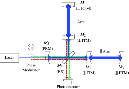
Figure 1: Schematic configuration of the initial LIGO detector, a power-recycled Fabry-Perot Michelson interferometer (PRFPMI).

In Fig. 1, we show the configuration of the initial LIGO detector, a power-recycled Fabry-Perot Michelson interferometer (PRFPMI). The light from a stabilized laser source enters the interferometer, which is comprised of an asymmetric Michelson interferometer with Fabry-Perot arm cavities. The arm cavities consist of polished input and end test masses (ITM and ETM, respectively) whose coated surfaces also act as mirrors to resonantly enhance the laser light. An additional power-recycling mirror (PRM) placed between the laser and beamsplitter increases the total light power available to the arms, by forming a “recycling cavity” together with the beamsplitter and arm cavity input mirrors. The sideband frequency and interferometer lengths are adjusted so that the sidebands resonate in the recycling cavity but not in the arms, while the carrier resonates in both sets of cavities. This allows extraction of control signals for all four length degrees of freedom.fri01

The noise level in the detection band at the interferometer output port must be held below the required strain sensitivity. The primary noise sources limiting the interferometer sensitivity are seismic noise at frequencies below 100 Hz, thermal noise between roughly 100 and 300 Hz, and photon counting noise at frequencies greater than 300 Hz. Photon counting noise is suppressed by using sufficient laser power; a design strain sensitivity of roughly 10^-21 over a time period of a millisecond will require a power of several hundred watts incident on the beamsplitter.

A concern in the operation of an interferometer at such high power levels is optical distortion. The presence of absorption in the coatings and substrates of the optics can give rise to non-uniform heating due to the Gaussian intensity profile of the laser light. This heating will cause a temperature rise in the substrate, which, coupled to the temperature dependence of the substrate index of refraction, will cause a distortion of the wavefront of the light transmitted through the substrate. For example, the initial LIGO design provides for fused silica input test masses which are 10 cm thick. To ensure the stability of the arm cavity resonant mode, the ITM radius of curvature is set to be several times the length of the arm cavity, or of order 10 km. By comparison, the substrate heating due to a nominal substrate and coating absorption of 5 ppm/cm and 1 ppm respectively causes the generation of a thermal lens in the substrate with a nominal focal length of 8 km. This significant distortion can have important consequences for both the power buildup of the RF sidebands in the recycling cavity and the interferometer sensitivity.

There have been a number of efforts made to understand the effects of the propagation of distorted wavefronts through gravitational wave interferometers, including an approximate treatment of wavefront distortion in power-recycled and dual-recycled systems due to imperfections in the shape or alignment of some optical components,mee91 an approximate treatment of thermal lensing and surface deformation in early Fabry-Perot Michelson designs,win91 and an approximate description of thermal lensing in alternate signal extraction designs.str94 ; mcc99 Each of these discussions emphasized the effects of optical distortion on a particular subset of the optical performance characteristics of an interferometer. In principle, fast Fourier transform methodsfft92 ; fft97 ; fft98 can be used to simulate a thermally loaded interferometer, but the computational cost of an iterated self-consistent FFT numerical analysis of the corresponding intracavity fields would be prohibitive.

By contrast, we have developed a flexible and robust analytical and numerical model of the effects of wavefront distortion on the optical performance of a gravitational-wave interferometer that requires far fewer computational resources than an FFT approach. The model includes accurate contributions to the thermal distortions in all substrates due to optical absorption in the substrate and both coatings of each test mass,hel90a the effects of any mismatch between the curvatures of the laser wavefront and the mirror surface at each reflection, and the diffraction by an aperture at each instance of reflection and transmission. Operators representing these physical effects on the reflection and transmission properties of mirrors and beamsplitters are explicitly incorporated into a set of transfer (or scattering) matrices that relate output fields to input fields incident on the surfaces of those elements. The corresponding transfer matrices of more complex optical components (e.g., a Fabry-Perot interferometer) can subsequently be constructed in a hierarchical fashion from those of simpler systems. Using this approach, the model determines a self-consistent steady-state solution to the interferometer power buildup in the presence of optical distortion, and employs an internal numerical mechanism to preserve the nearly ideal longitudinal phase resonance conditions that would otherwise be provided by an external servo-locking control system. We have developed computer code representing this model that is sufficiently flexible to allow new physical effects to be added to the simulations with a modicum of effort, and that can be stopped, interrogated, and restarted at any stage of a simulation. Our implementation of the artificial resonance-locking mechanism provides an exponential reduction in the execution time required for a self-consistent simulation by dynamically adjusting the frequency response of the interferometer.

Our current model employs basis function expansions of the electromagnetic field everywhere in the interferometer.and84 ; mor94 ; hef96 ; bea99 In principle, these basis functions can be spatial eigenfunctions of the interferometer, but in practice, imperfect mode-matching of the multiple cavities comprising the full interferometer and the presence of apertures in the system means that round-trip spatial propagators are not Hermitian, and the eigenfunctions are not power-orthogonal.sie86 ; oug87 ; kos97 Therefore, we choose an expansion of the intracavity field in an arbitrary set of power-orthogonal unperturbed spatial basis functions that are not necessarily eigenfunctions of any subsystem of a thermally loaded, perturbed interferometer. Since we can move from one spatial representation to another simply by recomputing the propagator matrix elements, the relative merit of a set of possible basis choices is determined by the number of basis modes needed to describe the intracavity field accurately. Our analysis of the operators encapsulating the physics of the perturbative phenomena described in the model is invariant under such a change of spatial basis. Nevertheless, the choice of an incomplete subset of basis functions inevitably introduces false optical losses because power is transferred to higher-order spatial modes which are not included in a necessarily finite numerical simulation. Therefore, we introduce unitary approximations for non-diffractive operators that monotonically improve as more basis functions are included in the simulation.

In Section II of this paper, we describe our representation of the intracavity electromagnetic field, and the operators incorporated into the transfer matrices of the subsystems comprising components of typical interferometric gravitational wave detectors. We develop a unitary approximation for non-diffractive operators expanded in finite-dimensional basis sets, and, in our discussions of the Fabry-Perot and Michelson interferometers, we introduce abstract idealizations of the control systems needed to maintain different intracavity resonance conditions. In Section III, using these building blocks we construct a model of the initial LIGO interferometer, and we point out that the basis functions chosen for a matrix description of the interferometer need not be spatial eigenfunctions of the fully coupled resonators. As a preliminary verification of our method, we compare the predictions of our numerical implementation of this model in a set of well-defined linear test cases with the output generated by a fast Fourier transform computer code suite. Finally, we simulate the optical performance of the initial LIGO interferometer under full thermal load, using a straightforward nonlinear solution method that computes the steady-state fields everywhere in the system after only a few seconds on an ordinary desktop computer.

II Models of Optical Components and Structures

II.1 Representation of the Electromagnetic Field

Throughout this work, we represent a propagating laser electric field ${\bf E}({\bf r},t)$ with angular carrier frequency $\omega_{0}$ as the real part of a product of a real time-independent polarization unit vector ${\bf e}$, a complex amplitude function $E({\bf r},t)$, and the carrier wave function $\exp\left[i(k_{0}z-\omega_{0}t)\right]$, where $\lambda_{0}\equiv 2\pi/k_{0}\equiv 2\pi c/\omega_{0}$ is the laser wavelength:bea99

$${\bf E}({\bf r},t)\equiv{\rm Re}\left\{{\bf e}\,E({\bf r},t)\exp\left[i(k_{0}z-\omega_{0}t)\right]\right\}.$$ (1)

We use the amplitude function $E({\bf r},t)$ to represent any closely-spaced frequency components (such as radio-frequency-modulated sidebands) as

$$E({\bf r},t)\equiv\sum_{q}E_{q}({\bf r},t)\exp\left[i(k_{q}z-\omega_{q}t)\right],$$ (2)

where the summation is taken over all frequency components (including the carrier), $E_{q}({\bf r},t)$ is the complex amplitude function of component $q$, and $\Delta\omega_{q}\equiv\omega_{q}-\omega_{0}\equiv\Delta k_{q}/c\ll\omega_{0}$ is the angular frequency shift of component $q$. By convention, the carrier is labeled by $q=0$, and therefore $\Delta\omega_{0}=0$. We express all field amplitudes in units of $\sqrt{{\rm W}/{\rm cm}^{2}}$, so that the time-averaged intensity carried by ${\bf E}({\bf r},t)$ is $\bar{I}({\bf r},t)=\frac{1}{2}\sum_{q}|E_{q}({\bf r},t)|^{2}$.

We will represent the transverse spatial dependence of the field amplitude $E_{q}({\bf r},t)$ at any propagation plane within a laser interferometric gravitational-wave detector as a linear superposition of a set of amplitude basis functions with fixed transverse spatial profiles. In general, these amplitudes are eigenfunctions of a non-Hermitian integral transform equation (generally a composition of many consecutive integral transforms, each of which carries the field from one aperture to the next) that describes round-trip propagation through a specific resonant subsystem of the unperturbed interferometer. These resonant eigenfunctions can then be propagated throughout the remainder of the interferometer, defining a unique set of spatial basis functions.bea99 Therefore, given the existence of a numerically complete set of these transverse spatial eigenfunctions, we can expand the sideband amplitude function as

$$E_{q}({\bf r},t)=\sum_{mn}E_{mnq}(z,t)\,u_{mn}({\bf r}).$$ (3)

Hence, we can convert any composition of two consecutive integral transforms into a simple matrix product. In practice, we are interested in the steady-state characteristics of the detector under thermal load, and we will clearly indicate the propagation plane under discussion, so we will usually suppress the explicit coordinates $\{z,t\}$ in later sections.

As an example, consider the simple case of laser field propagation through a distance $L\equiv z_{2}-z_{1}$ in vacuum. Suppose that we choose to represent the spatial and temporal properties of this field using $N$ transverse eigenfunctions $u_{mn}({\bf r})$ and $Q$ frequency components, including the carrier and both positive and negative sidebands for each nonzero radio modulation frequency. We arrange the expansion coefficients into an $N\times Q$ ordered matrix $E$ with elements $E_{mnq}$, where each row represents the spatial eigenfunction corresponding to a particular choice of $\{m,n\}$ and each column corresponds to a particular frequency component $q$, and we assume that $L$ has been chosen to provide resonant excitation of the fundamental carrier spatial mode $E_{000}$. In this basis, the spatial contribution to the vacuum propagation kernel is given by a $N\times N$ diagonal matrix $G$ with elements

$$G_{mn,m^{\prime}n^{\prime}}=\exp(i\,\Delta\,\varphi_{mn})\,\delta_{mm^{\prime}}\,\delta_{nn^{\prime}},$$ (4)

where $\Delta\,\varphi_{mn}\equiv\varphi_{mn}-\varphi_{00}$ is the net Gouy phase (relative to the fundamental spatial mode) accumulated by mode $mn$ over the propagation distance $L$, and the net longitudinal optical path length contribution (relative to the carrier) is given by a $Q\times Q$ diagonal matrix $\Omega$ with elements

$$\Omega_{qq^{\prime}}=\exp(i\Delta\omega_{q}\tau)\,\delta_{qq^{\prime}},$$ (5)

where $\tau\equiv L/c$ is the propagation time. The components of the field following the propagation step can then be computed using the sparse matrix product

$$E(z_{2})=G\,E(z_{1})\,\Omega.$$ (6)

We are particularly interested in the more complex example of a power-recycled Fabry-Perot Michelson laser gravitational-wave interferometer. In its unperturbed state (i.e., in the absence of aperture diffraction and thermal wavefront distortions), this detector configuration is described well by Hermite-Gauss basis functions under perfect mode-matching conditions. The infinite-aperture Hermite-Gauss basis is orthonormal (since it is generated by a Hermitian propagation equation), so that field amplitude expansions using this basis are power orthogonal,sie86 allowing time-averaged intensities to be calculated using the sum of the inner products $|E_{q}({\bf r},t)|^{2}=\sum_{m\,n}\,|E_{mnq}(z,t)|^{2}$. If both Gouy and optical path length phase contributions are accumulated using Eq. (6), then we can represent an arbitrary non-astigmatic Hermite-Gauss basis function $u_{mn}(x,y)$ at a given reference plane using

$$\begin{split}u_{mn}(x,y)&=\left(\frac{1}{2^{m+n}m!n!}\,\frac{2}{\pi\,w^{2}}\right)^{1/2}\\ &\times H_{m}\left(\frac{\sqrt{2}x}{w}\right)\,H_{n}\left(\frac{\sqrt{2}y}{w}\right)\,\\ &\times\exp\left[\left(i\frac{k}{2R}-\frac{1}{w^{2}}\right)\left(x^{2}+y^{2}\right)\right],\end{split}$$ (7)

where $H_{n}(x)$ is the Hermite polynomial of order $n$, $w$ is the beam spot radius, and $R$ is the wavefront radius of curvature at that reference plane. Throughout this work, we will define the $x$-$z$ plane to be “horizontal,” containing the central beam paths of the two Fabry-Perot arm cavities in Fig. 1, and the $y$-$z$ plane to be “vertical,” perpendicular to the horizontal plane and parallel to the local gravity gradient of the Earth.

II.2 Mirrors

II.2.1 Aperture Diffraction and Mirror-Field Curvature Mismatch Operators

Consider the general problem of the reflection of a propagating electromagnetic field by a perfectly reflecting cylindrically symmetric mirror $\mathcal{M}$ with spherical radius of curvature $R_{M}$ and aperture diameter $2a$. The reflection can be described in a single step taken from the aperture $\mathcal{A}$ at the reference plane $z^{<}$ conventionally located just before the reflection from $\mathcal{M}$ to the field position $z^{>}$ just after reflection has occurred. If the transverse field at $z^{<}$ is $E(x^{\prime},y^{\prime},z^{<})$, then the corresponding field at $z^{>}$ is given by Huygens’s integral in the Fresnel approximation asoug87

$$E(x,y,z^{>})=\int_{\mathcal{A}}dx^{\prime}\,dy^{\prime}\,K(x,y;x^{\prime},y^{\prime})E(x^{\prime},y^{\prime},z^{<}),$$ (8)

where the functional form of the forward propagation kernel for a cylindrically symmetric mirror isbea99

$$\begin{split}K(x,y;x^{\prime},y^{\prime})&=-\exp\left[-i\,\frac{\pi}{\lambda_{0}}\frac{2}{R_{M}}\left({x^{\prime}}^{2}+{y^{\prime}}^{2}\right)\right]\\ &\times\,\delta(x-x^{\prime})\,\delta(y-y^{\prime}).\end{split}$$ (9)

Here the leading negative sign accounts for the Maxwell boundary condition at the perfectly reflecting mirror surface.

If we expand the field at both reference planes using a numerically complete set of cartesian basis functions as in Eq. (3), then we can compute the matrix elements of the forward propagation kernel in that basis as

$$\begin{split}K_{mn,m^{\prime}n^{\prime}}&=\iint\limits^{\quad\;\infty}_{-\infty}dx\,dy\,\iint_{\mathcal{A}}dx^{\prime}\,dy^{\prime}\;K(x,y;x^{\prime},y^{\prime})\\ &\qquad\times\,u^{\dagger}_{mn}(x,y,z^{>})\,u_{m^{\prime}n^{\prime}}(x^{\prime},y^{\prime},z^{<})\\ &=\iint_{\mathcal{A}}dx\,dy\;\exp\left[-i\,\frac{\pi}{\lambda_{0}}\frac{2}{R_{M}}\left(x^{2}+y^{2}\right)\right]\\ &\qquad\times\,u^{\dagger}_{mn}(x,y,z^{>})\,u_{m^{\prime}n^{\prime}}(x,y,z^{<})\end{split}$$ (10)

Here the function $u^{\dagger}_{mn}(x,y,z^{>})$ is not generally the conjugate transpose of $u_{mn}(x,y,z^{>})$. Instead, these basis functions represent fields propagating through the system in the reverse direction, and are obtained by solving the Huygens-Fresnel integral Eq. (8) using $K^{T}(x,y;x^{\prime},y^{\prime})$, the transpose of the forward-propagation kernel.bea99 ; oug87 ; sie86

Although the reflection-diffraction problem is specified completely by Eq. (10), it can introduce inconsistencies in practical implementations of optical resonator simulations. For example, when a finite number of basis functions are used to represent the propagating field, the matrix calculated using Eq. (10) generates two sources of optical loss: genuine diffraction loss due to field truncation by the aperture, and power transferred to higher-order optical modes which are ignored in the simulation. The latter contribution is unphysical: in the limit $a\rightarrow\infty$, when a numerically complete set of basis functions is used the propagation matrix must conserve energy (i.e., must be unitary.) Therefore, for the purposes of our simulations we will explicitly allow diffraction loss due to aperture truncation only, and separate the effects of aperture diffraction and reflection into two consecutive propagation steps using the formulation

$$K\cong C\,A,$$ (11)

where $A$ is a matrix operator representing purely transmissive aperture diffraction, and $C$ is a unitary matrix operator describing direct focusing by a spherical mirror at normal incidence.

As a concrete example, we first calculate the matrix elements of $A$ in the Hermite-Gauss basis, treating the truncation as a perturbation and describing the field both before and after the aperture using a linear superposition of a finite set of unperturbed Hermite-Gauss functions. Therefore, $u^{\dagger}_{mn}(x,y)=u^{*}_{mn}(x,y)$, and we define the analytical integral

$$\begin{split}A_{mn,m^{\prime}n^{\prime}}&=\iint_{\mathcal{A}}dx\,dy\;u^{*}_{mn}(x,y)\,u_{m^{\prime}n^{\prime}}(x,y)\\ &\equiv\delta_{m,m^{\prime}}\,\delta_{n,n^{\prime}}-e^{-\alpha}\,I_{mn,m^{\prime}n^{\prime}}(\alpha),\end{split}$$ (12)

where $\alpha\equiv 2(a/w)^{2}$, and the integration is performed over the circular aperture defined by $\sqrt{x^{2}+y^{2}}\leq a$. We specify a basis set by designating the transverse modes for a given frequency component $q$ in order of increasing $m+n$ first, and then in order of increasing $n$. For example, if we use a Hermite-Gauss basis with $m+n\leq 2$, then for the column vector $E_{q}\equiv\{E_{00q},E_{10q},E_{01q},E_{20q},E_{11q},E_{02q}\}^{T}$ we obtain the matrix

$$I(\alpha)=\begin{bmatrix}1&0&0&\frac{1}{\sqrt{2}}\alpha&0&\frac{1}{\sqrt{2}}\alpha\\ 0&1+\alpha&0&0&0&0\\ 0&0&1+\alpha&0&0&0\\ \frac{1}{\sqrt{2}}\alpha&0&0&1+\frac{1}{2}\alpha+\frac{3}{4}\alpha^{2}&0&\frac{1}{4}\alpha(\alpha-2)\\ 0&0&0&0&1+\alpha+\frac{1}{2}\alpha^{2}&0\\ \frac{1}{\sqrt{2}}\alpha&0&0&\frac{1}{4}\alpha(\alpha-2)&0&1+\frac{1}{2}\alpha+\frac{3}{4}\alpha^{2}\end{bmatrix},$$ (13)

Note that nonzero elements of $I(\alpha)$ satisfy the relation $I_{mn,m^{\prime}n^{\prime}}(\alpha)\approx O[\alpha^{\frac{1}{2}(m+n+m^{\prime}+n^{\prime})}]$.

Next, we ignore aperture diffraction and calculate the matrix elements of $C$ in the Hermite-Gauss basis. Strictly speaking, the matrix elements of $C$ can be calculated using Eq. (10) in the limit $a\rightarrow\infty$. However, as described above, we seek an explicitly unitary approximation for $C$ that monotonically improves as we include more basis functions in the field expansion. When Eq. (10) is applied to a Hermite-Gauss basis function with field curvature parameter $R_{F}$, this parameter is transformed according to the $ABCD$ propagation law as $1/R_{F}^{\prime}=1/R_{F}-2/R_{M}$. In the unperturbed case where $R_{M}=R_{F}$, the curvature parameter of the backward-propagating basis function is therefore $-(-R_{F})=R_{F}$, and using Eq. (7) we have

$$C\cong\exp(i\,\gamma\,c),$$ (14)

where

$$\gamma\equiv\frac{\pi\,w^{2}}{\lambda}\left(\frac{1}{R_{F}}-\frac{1}{R_{M}}\right),$$ (15)

and

$$\begin{split}c_{mn,m^{\prime}n^{\prime}}&\equiv\frac{2}{w^{2}}\iint\limits^{\quad\;\infty}_{-\infty}dx\,dy\;\,\left(x^{2}+y^{2}\right)\\ &\times\,\left|u_{mn}(x,y)\,u_{m^{\prime}n^{\prime}}(x,y)\right|.\end{split}$$ (16)

As the number of Hermite-Gauss basis functions used to represent $E_{q}$ grows, $\exp(i\,\gamma\,c)\rightarrow C$, and since $c$ is symmetric, $\exp(i\,\gamma\,c)$ is explicitly unitary. Using the generating function of the Hermite polynomials, we obtain the matrix elements

$$c_{mn,m^{\prime}n^{\prime}}=X^{2}_{m,m^{\prime}}\,\delta_{n,n^{\prime}}+\delta_{m,m^{\prime}}\,X^{2}_{n,n^{\prime}},$$ (17)

where

$$\begin{split}X^{2}_{m,m^{\prime}}&\equiv\frac{1}{2}(1+2m)\,\delta_{m,m^{\prime}}\\ &+\frac{1}{2}\sqrt{(m^{\prime}+1)(m^{\prime}+2)}\;\delta_{m,m^{\prime}+2}\\ &+\frac{1}{2}\sqrt{(m+1)(m+2)}\;\delta_{m^{\prime},m+2}.\end{split}$$ (18)

As a straightforward test of our unitary approximation, we can compare the separated propagator given by Eq. (11) with the exact propagator specified by Eq. (10) for the TEM₀₀ Hermite-Gauss mode. An explicit calculation using Eq. (10) yields

$$K_{00,00}=\frac{1-e^{-(1+i\gamma)\alpha}}{1+i\gamma}.$$ (19)

In Fig. 2, we plot the fractional error in $|K_{00,00}|$ accrued by computing $K=C\,A$, where $A$ is provided by Eq. (12) and $C$ by Eq. (14). For an incident field with a spot radius $w=3.64$ cm and a wavefront radius of curvature $R_{F}=10$ km at a wavelength $\lambda=1.0642$ $\mu$m, we show relative errors for different values of the mirror’s cylindrical substrate radius and radius of curvature as a function of the maximum mode index $N$. The number of basis modes with $m+n\leq N$ used in the calculations of $A$ and $C$ is given by $\frac{1}{2}(N+1)(N+2)$. As we expect, the relative error decreases significantly as the number of basis modes increases.

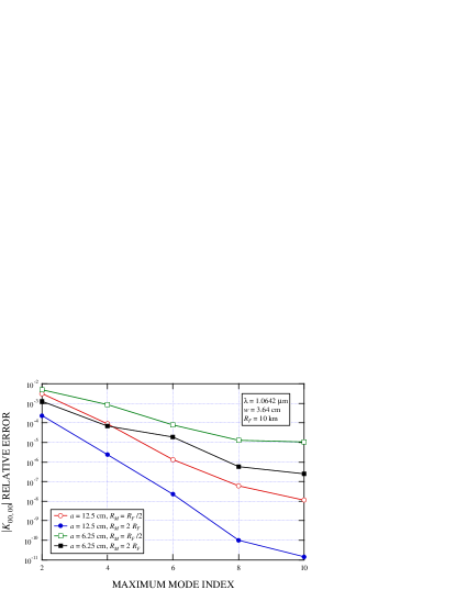
Figure 2: The fractional error in $|K_{00,00}|$ obtained by comparing the exact value given by Eq. (19) with the TEM₀₀ element of the approximate propagator $K=C\,A$, where $A$ is provided by Eq. (12) and $C$ by Eq. (14).

II.2.2 Thermal Focusing Operators

In an interferometric gravitational-wave detector, the test masses (as well as any optics which form power and/or signal recycling cavities) are thick cylindrical blocks of a transparent material, such as pure fused silica. A high-reflectance coating (HR) is applied to the broad inner face of the cylinder, forming a mirror; if transmission through the mirror substrate is necessary, then an antireflecting coating (AR) will be applied to the outer surface as well. Under test, then, laser power may be absorbed in the coatings and/or the mirror substrate (SS), and the corresponding heat flow into the substrate will result in an inhomogeneous temperature distribution throughout the mirror. This temperature gradient will cause a refractive index gradient to form, converting the substrate into a thermally-generated thick lens.

In general, the propagation of the laser field through the substrate will be described by an integral transform equation that incorporates the effects of position-dependent optical phase shifts caused by the thermal load. As discussed above, by choosing a suitable set of unperturbed basis functions (i.e., in the absence of thermal and mechanical perturbations) we can convert the integral transform equation into a scattering matrix operator which redistributes energy contained in an initial configuration of basis functions into the final set of corresponding functions that emerges from the substrate. In order to determine the elements of this matrix operator, we must first find the temperature distribution in the substrate due to absorption in both the coatings and the substrate, and then we must compute the matrix elements of the longitudinal optical path-difference (OPD) phase shift introduced by the temperature gradient.

Hello and Vinethel90a have calculated both the steady-state and transient temperature distribution throughout the simplified mirror shown in Fig. 3 for the case where the change in the temperature due to the absorption of optical power remains small compared to the external ambient temperature $T_{0}$. This assumption linearizes the radiative boundary conditions at the surfaces of the mirror, and allows the temperature increase due to coating and substrate absorption to be calculated independently (and then summed) for some incident power $P$. As shown in Fig. 3, they treated the mirror substrate as a thick disk spanning the cylindrical coordinates $0\leq r\leq a$ and $-h/2\leq z\leq h/2$, and the coating is concentrated in an infinitesimally thin layer at $z=-h/2$. After an algebraic simplification of Hello and Vinet’s steady-state results, we find that the temperature distributions throughout the substrate due to absorption in the substrate and coating are, respectively,

$$\begin{split}T_{s}(r,z)&=P\,\frac{\alpha_{s}a^{2}}{k_{T}}\sum_{k}\frac{p_{k}}{\zeta_{k}^{2}}\\ &\times\biggl{[}1-2\tau A_{k}\cosh\left(\zeta_{k}\,\frac{z}{a}\biggr{)}\right]J_{0}\left(\zeta_{k}\,\frac{r}{a}\right),\end{split}$$ (20)

$$\begin{split}&T_{c}(r,z)=P\,\frac{a_{c}a}{k_{T}}\sum_{k}p_{k}\\ &\times\,\biggl{[}A_{k}\cosh\left(\zeta_{k}\,\frac{z}{a}\right)-B_{k}\sinh\left(\zeta_{k}\,\frac{z}{a}\right)\biggr{]}J_{0}\left(\zeta_{k}\,\frac{r}{a}\right),\end{split}$$ (21)

where $a_{c}$ is the power absorption of the coating, $\alpha_{s}$ is the absorption coefficient of the substrate material,

$$A_{k} = \frac{1}{2\left[\zeta_{k}\sinh\left(\gamma_{k}\right)+\tau\cosh\left(\gamma_{k}\right)\right]},$$ (22a)

$$B_{k} = \frac{1}{2\left[\zeta_{k}\cosh\left(\gamma_{k}\right)+\tau\sinh\left(\gamma_{k}\right)\right]},$$ (22b)

$\gamma_{k}\equiv\zeta_{k}h/2a$, $\tau\equiv 4\epsilon\sigma T_{0}^{3}a/k_{T}$, $\sigma$ is the Stefan-Boltzmann constant, $\epsilon$ is the total spherical emissivity of the substrate, and $k_{T}$ is the thermal conductivity of the substrate. For $a=12.5$ cm (consistent with the value chosen for the LIGO test masses) and $T_{0}=300$ K, we have $\tau=0.277$. The terms in these series are characterized by the roots of the equation

$$\zeta J_{1}\left(\zeta\right)-\tau J_{0}\left(\zeta\right)=0,$$ (23)

which are reasonably well-approximated by the zeros of $J_{1}\left(\zeta\right)$, $\zeta_{k}\cong(k+1/4)\pi$ for $k\in\{0,1,2,\ldots\}$, when $\tau<1$.

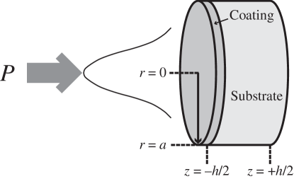
Figure 3: Schematic diagram of a singly-coated mirror and the corresponding coordinate system used by Hello and Vinethel90a . Both the mirror and the incident power distribution are assumed to be azimuthally symmetric. The total incident power $P$ can be absorbed in the coating and/or the substrate, resulting in a total temperature distribution $T(r,z)$ and a corresponding thermal lens in the substrate.

The constants $p_{k}$ are the coefficients of a Dini series expansionhel90a of the azimuthally symmetric incident intensity distribution $I(r)$, given by

$$I(r)\equiv\sum_{k}p_{k}\,J_{0}\left(\zeta_{k}\,\frac{r}{a}\right).$$ (24)

A straightforward calculation using Eq. (23) yields

$$p_{k}=\frac{2\zeta_{k}^{2}}{\left(\zeta_{k}^{2}+\tau^{2}\right)J_{0}^{2}\left(\zeta_{k}\right)}\frac{1}{a^{2}}\int_{0}^{a}dr\,r\,J_{0}\left(\zeta_{k}\,\frac{r}{a}\right)I(r).$$ (25)

If we assume that the field is primarily comprised of the fundamental $\{00\}$ mode, then we can neglect the slight heating arising from higher-order modes. When the incident intensity describes a unit power TEM₀₀ Gaussian beam with spot radius $w$, we have $I(r)=(2/\pi w^{2})\exp\left(-2r^{2}/w^{2}\right)$. Furthermore, if $w/a\ll 1$, we can extend the upper limit of integration in Eq. (25) to infinity, thereby obtaining the analytic expression

$$p_{k}=\frac{1}{\pi a^{2}}\frac{\zeta_{k}^{2}}{\left(\zeta_{k}^{2}+\tau^{2}\right)J_{0}^{2}\left(\zeta_{k}\right)}\exp(-\beta_{k}),$$ (26)

where $\beta_{k}\equiv\frac{1}{8}(\zeta_{k}w/a)^{2}$.

The $z$ dependence of the substrate temperature distribution given by Eq. (20) is typically very weak when $w/a\ll 1$ and the boundary conditions are radiative.hel90a In this case, near $r=0$ we can use the identity $\sum_{k}p_{k}=I(0)=2/\pi w^{2}$ to obtain the approximate temperature distribution $T_{s}(r)-T_{s}(0)\cong(\alpha_{p}P_{s}/2\pi k_{T})(r/w)^{2}$. In the thin lens approximation, this quadratic temperature gradient yields a weak focal lengthsie86

$$f=\frac{\pi w^{2}}{\alpha_{s}hP}\,\frac{k_{T}}{d\eta/dT}.$$ (27)

The material constants for fused silica are shown in Table 1. If we assume typical LIGO parameter values for the test masses, then we have $w=4$ cm, $h=10$ cm, and $P=500$ W, giving $f=16$ km, a length only four times greater than that of a LIGO Fabry-Perot arm cavity.

Table 1: Material constants for fused silica used in our simulations.

Constant	Name	Value	Units
$\eta$	Refractive index	1.44968
$d\eta/dT$	First-order $\eta$-$T$ coefficient	$8.7\,\times\,10^{-6}$	K-1
$k_{T}$	Conductivity	1.38	W/m K
$\epsilon$	Total spherical emissivity	0.76
$\alpha_{s}$	Bulk absorption coefficient	$5\,\times\,10^{-4}$	m-1
$\sigma_{s}$	Bulk scattering coefficient	$0.5\,\times\,10^{-4}$	m-1

The thermal load on the substrate causes a position-dependent phase shift across any wavefront propagating through the mirror. Defining the longitudinal optical path-difference (OPD) phase $\phi$ as

$$\phi(r)\equiv\frac{2\pi}{\lambda_{0}}\frac{d\,\eta}{d\,T}\int_{-h/2}^{h/2}dz\ T(r,z),$$ (28)

we obtain for the substrate and coating contributions

$$\phi_{s}(r) = P_{s}\,\frac{2\pi a^{2}}{\lambda_{0}k_{T}}\frac{d\,\eta}{d\,T}\sum_{k}\frac{p_{k}}{\zeta_{k}^{2}}$$ (29a)

$$\times \left[1-\frac{2\tau A_{k}}{\gamma_{k}}\sinh\left(\gamma_{k}\right)\right]J_{0}\left(\zeta_{k}\,\frac{r}{a}\right),$$

$$\phi_{c}(r) = P_{c}\,\frac{2\pi a^{2}}{\lambda_{0}k_{T}}\frac{d\,\eta}{d\,T}\sum_{k}\frac{p_{k}}{\zeta_{k}}$$ (29b)

$$\times 2A_{k}\sinh\left(\gamma_{k}\right)J_{0}\left(\zeta_{k}\,\frac{r}{a}\right),$$

where $P_{s}\equiv\alpha_{p}hP$ and $P_{c}\equiv a_{c}P$ are the powers absorbed in the substrate and coating, respectively. If the thickness of the substrate is small compared to the wavefront radius of curvature, then we can approximate the propagator describing transmission through the substrate as a diffraction step through the aperture followed by a direct integration of the OPD across the aperture to describe the accumulated distortion. If we define the “edge-to-center” OPD phase as $\Delta\phi(r)\equiv\phi(r)-\phi(0)$, then we can compute the total substrate thermal distortion matrix operator using

$$\begin{split}S_{mn,m^{\prime}n^{\prime}}&=\iint\limits^{\quad\;\infty}_{-\infty}dx\,dy\;\exp\left[i\Delta\phi(r)\right]\\ &\times\,u_{mn}^{\dagger}(x,y)\,u_{m^{\prime}n^{\prime}}(x,y)\end{split}$$ (30)

for both substrate and coating absorption.

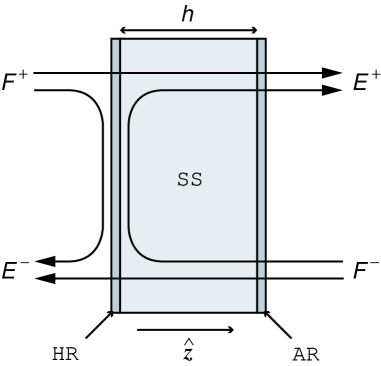
Figure 4: Schematic diagram of field distributions in a mirror of thickness $h$, consisting of a substrate (SS) with applied high-reflectance (HR) and antireflecting (AR) coatings.

As we discussed above for the wavefront-mirror curvature matrix $C$ given by Eq. (14), we seek a unitary approximation of the substrate thermal distortion matrix to ensure that power is conserved even when a finite set of unperturbed basis functions is used to compute the matrix elements. Once again, we begin by computing the matrix elements of the exponential arguments $\Delta\phi_{s}(r)$ and $\Delta\phi_{c}(r)$ as

$$\Phi_{s;mn,m^{\prime}n^{\prime}} = P_{s}\,\frac{2\pi a^{2}}{\lambda_{0}k_{T}}\frac{d\,\eta}{d\,T}\sum_{k}\frac{p_{k}}{\zeta_{k}^{2}}\biggl{[}1$$ (31a)

$$- \frac{\tau}{\gamma_{k}}\,2A_{k}\sinh\left(\gamma_{k}\right)\biggr{]}e^{-\beta_{k}}I_{k;mn,m^{\prime}n^{\prime}}$$

$$\Phi_{c;mn,m^{\prime}n^{\prime}} = P_{c}\,\frac{2\pi a^{2}}{\lambda_{0}k_{T}}\frac{d\,\eta}{d\,T}\sum_{k}\frac{p_{k}}{\zeta_{k}}\,$$ (31b)

$$\times 2A_{k}\sinh\left(\gamma_{k}\right)e^{-\beta_{k}}I_{k;mn,m^{\prime}n^{\prime}}.$$

where we have defined the matrix integral $I_{k}$ as

$$\begin{split}I_{k;mn,m^{\prime}n^{\prime}}&\equiv e^{\beta_{k}}\iint\limits^{\quad\;\infty}_{-\infty}dx\,dy\;\left[J_{0}\left(\zeta_{k}\,\frac{r}{a}\right)-1\right]\\ &\times\,u_{m^{\prime}n^{\prime}}^{\dagger}(x,y)\,u_{mn}(x,y).\end{split}$$ (32)

Since the integrand is zero at $r=\sqrt{x^{2}+y^{2}}=0$, our definition of $\Delta\phi(r)$ allows us to explicitly ignore any phase shift accumulated due to the peak thermal change in the substrate refractive index, and instead we include only the contribution to the wavefront distortion arising from the shape of the temperature distribution. Using the same example Hermite-Gauss basis described in Section II.2.1, for $m+n\leq 2$ and a given value of $k$, we obtain the square matrix elements

$$I_{k}(\beta_{k})=\begin{bmatrix}1&0&0&-\,\frac{1}{\sqrt{2}}\,\beta_{k}&0&-\,\frac{1}{\sqrt{2}}\,\beta_{k}\\ 0&1-\beta_{k}&0&0&0&0\\ 0&0&1-\beta_{k}&0&0&0\\ -\,\frac{1}{\sqrt{2}}\,\beta_{k}&0&0&1-2\beta_{k}+\frac{3}{4}\beta_{k}^{2}&0&\frac{1}{4}\beta_{k}^{2}\\ 0&0&0&0&1-2\beta_{k}+\frac{1}{2}\beta_{k}^{2}&0\\ -\,\frac{1}{\sqrt{2}}\,\beta_{k}&0&0&\frac{1}{4}\beta_{k}^{2}&0&1-2\beta_{k}+\frac{3}{4}\beta_{k}^{2}\end{bmatrix},$$ (33)

Note that nonzero elements of $I_{k}(\beta_{k})$ satisfy the relation $I_{k;mn,m^{\prime}n^{\prime}}(\beta_{k})\approx O[\beta_{k}^{\frac{1}{2}(m+n+m^{\prime}+n^{\prime})}]$.

Collecting results, we can compute the net effective substrate OPD matrix operator in our unitary approximation as

$$S=\exp\left\{i\,\left[P_{s}\,\Phi_{s}+\left(P_{h}+P_{a}\right)\Phi_{c}\right]\right\},$$ (34)

where $P_{s}$, $P_{h}$, and $P_{a}$ are the total TEM₀₀ optical powers absorbed in the substrate, HR coating, and AR coating, respectively. The power distribution throughout the mirror volume is shown schematically in Fig. 4 for a dual-coated cylindrical mirror with substrate thickness $h$. A laser field $F^{+}$ is incident on the HR coating (the “front” of the mirror), and another field $F^{-}$ is incident on the AR coating (the “back” of the mirror). Since we have assumed that the field is primarily comprised of the fundamental $\{00\}$ mode, then the total power absorbed in the coatings and substrate depend only on the field amplitude expansion coefficients $F_{00q}$, as listed in Table 2. Here $a_{\mathit{hr}}$ and $a_{\mathit{ar}}$ are the dimensionless fractional power absorptions of the HR and AR, respectively, and $\alpha_{s}$ is the power absorption coefficient of the substrate, with units of inverse length. The reflected field $E^{-}$ is the superposition of the prompt reflection of $F^{+}$ and the residual of $F^{-}$ which has been transmitted through the HR.

Table 2: Total absorbed TEM₀₀ powers for each of the three regions shown in Fig. 4, summed over the lowest-order transverse modes of all active sidebands. The factors of $\frac{1}{2}$ arise from our normalization convention for the laser electric field.

Region	Absorbed Power
SS	$P_{s}=\alpha_{s}h\,\frac{1}{2}\sum_{q}\left(|E^{+}_{00q}|^{2}+|F^{-}_{00q}|^{2}\right)$
HR	$P_{h}=a_{\mathit{hr}}\,\frac{1}{2}\sum_{q}\left(|F^{+}_{00q}|^{2}+|F^{-}_{00q}|^{2}\right)$
AR	$P_{a}=a_{\mathit{ar}}\,\frac{1}{2}\sum_{q}\left(|E^{+}_{00q}|^{2}+|F^{-}_{00q}|^{2}\right)$

II.2.3 Transfer Matrix

We can extend our analysis of the reflection and transmission processes and build a general transfer matrix for fields incident on the mirror from either direction. First, we choose the laser-industry standard conventions for the phases of the amplitude reflection and transmission coefficients for a quarter-wave dielectric stack. Therefore, the Maxwell boundary conditions for the HR generate the amplitude coefficients $-r$ for reflection and $i\,t$ for transmission, regardless of propagation direction. Losses in the HR due to absorption and scattering are included implicitly when $r^{2}+t^{2}<1$. However, we must explicitly account for losses due to transmission through the substrate and AR coating using the amplitude coefficient

$$t_{s}=e^{-(\alpha_{s}+\sigma_{s})h/2}\sqrt{1-(a_{ar}+s_{ar})},$$ (35)

where $\sigma_{s}$ is the scattering loss per unit length in the substrate, and $s_{ar}$ is the scattering loss in the AR coating.

The propagator for reflection from the vacuum side of the HR is given by Eq. (9), and the resulting perturbation matrix for a mismatch between the radius of curvature of the mirror and the wavefront is given by Eq. (14) as $C(\gamma)\equiv C^{-}$. Since the propagator for reflection from the substrate side of the HR is also given by Eq. (9) with $-2/R_{M}\rightarrow 2n/R_{M}$,sie86 where $n$ is the refractive index of the substrate, the corresponding perturbation matrix is $C(-n\,\gamma)\equiv C^{+}$. Similarly, the propagator for transmission through the HR from the substrate to the vacuum is given by Eq. (14) with $-2/R_{M}\rightarrow(n-1)/R_{M}$,sie86 so the transmission curvature mismatch matrix operator is $C[(n-1)\gamma/2]=(C^{-}C^{+})^{1/2}$.

In Section II.4.2 and Section III.2, we will adjust the microscopic positions of some of the mirrors to ensure that the perturbed interferometers maintain the appropriate resonant phase conditions as the system evolves. If the mirror in Fig. 4 is moved in the positive $\hat{z}$ direction (i.e., toward the right in the diagram) by the microdisplacement $\Delta z\lesssim\lambda$, then reflection from the “front” of the mirror introduces a relative phase $\exp(+i2k\Delta z)$, while reflection from the “back” of the mirror requires a phase adjustment of $\exp(-i2k\Delta z)$.

Collecting these results, the final mirror transfer matrix depicted in Fig. 5 is

$$\begin{bmatrix}E^{-}\\ E^{+}\end{bmatrix}=\begin{bmatrix}T^{-}&R^{-}\\ R^{+}&T^{+}\end{bmatrix}\,\begin{bmatrix}F^{-}\\ F^{+}\end{bmatrix},$$ (36)

where the transmission operators are

$$T^{-} = i\,t\,t_{s}\left(C^{-}C^{+}\right)^{1/2}S\,A,\text{ and}$$ (37a)

$$T^{+} = i\,t\,t_{s}\,S\left(C^{+}C^{-}\right)^{1/2}A,$$ (37b)

and the reflection operators are

$$R^{-} = -r\,e^{+i\,2k\,\Delta z}\,C^{-}\,A,\text{ and}$$ (38a)

$$R^{+} = -r\,t_{s}^{2}\,e^{-i\,2k\,\Delta z}\,S\,C^{+}\,S\,A.$$ (38b)

In the lossless case where $r^{2}+t^{2}=t^{2}_{s}=1$ and $A$ is the identity matrix, the explicit unitarity of the $C^{+}$, $C^{-}$, and $S$ matrix operators guarantees that $|E^{+}|^{2}+|E^{-}|^{2}=|F^{+}|^{2}+|F^{-}|^{2}$.

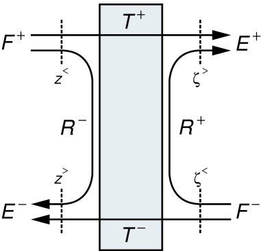
Figure 5: Schematic diagram of the generalized mirror transfer matrix given by Eq. (36). The HR-coated surface of the mirror is on the left. The labels $z^{<}$ and $z^{>}$ denote the input and output reference planes, respectively, near the HR surface, while $\zeta^{<}$ and $\zeta^{>}$ are the input and output reference planes near the AR surface.

II.3 Beamsplitter

II.3.1 Aperture Diffraction and Thermal Focusing Operators

The analysis of the aperture diffraction and thermal focusing operators for the case of a 45^∘ beamsplitter is similar to that of a mirror. However, even though the beamsplitter has the same cylindrically symmetric substrate as the mirror shown in Fig. 3, the non-normal angle of incidence will require the elements of the perturbative matrix operators to be computed numerically. We will assume here that the HR-coated surface of the beamsplitter is flat, allowing us to ignore both curvature mismatch and astigmatism when we build the transfer matrix in Section II.3.2.

The aperture diffraction operator for reflection from the HR-coated surface of the beamsplitter is given by

$$A_{mn,m^{\prime}n^{\prime}}=\iint_{\mathcal{E}}dx\,dy\;u^{\dagger}_{mn}(x,y)\,u_{m^{\prime}n^{\prime}}(x,y),$$ (39)

where $\mathcal{E}$ represents an elliptical aperture with semimajor ($y$) axis $a$ and semiminor ($x$) axis $a/\sqrt{2}$. Strictly speaking, the diffraction operator for transmission through the substrate is more complicated than Eq. (39) because of refraction at each vacuum-dielectric interface, particularly since the effective clear aperture (in the horizontal plane) after propagation through the substrate has been reduced by the distance $h/2\eta$, or about 1.4 cm for LIGO. In principle, we can construct separate operators for reflective and transmissive aperture diffraction, but in practice we have found that the resulting effect on the recycled power enhancement of the standard PRFPMI configuration shown in Fig. 1 was negligible. Hence, in our simulations, we have made the simplifying approximation that Eq. (39) can be used to represent aperture diffraction effects for both reflection and transmission.

The distribution of absorbed power within the beamsplitter volume is illustrated in Fig. 6, where we have introduced the primary propagation paths labeled parallel ($\parallel$) and perpendicular ($\perp$) relative to the propagation of the input laser field in Fig. 1. Following the conventions of Section II.2.2 as closely as possible, we then label the input fields incident on the front (HR-coated) side of the mirror with $\operatorname{sign}(\mathbf{\hat{k}\cdot\hat{z}})>0$ as $F^{+\parallel}$ and $F^{+\perp}$, and those incident on the back (AR-coated) side of the mirror, with $\operatorname{sign}(\mathbf{\hat{k}\cdot\hat{z}})<0$ as $F^{-\parallel}$ and $F^{-\perp}$. Together with the four corresponding output fields shown in Fig. 6, these fields generate five distinct optical power absorption regions. The total TEM₀₀ optical power absorbed in each of these regions is listed in Table 3, where $h^{\prime}\equiv h/\sqrt{1-1/2\eta^{2}}$ is the distance traveled through the substrate by the refracted beams.

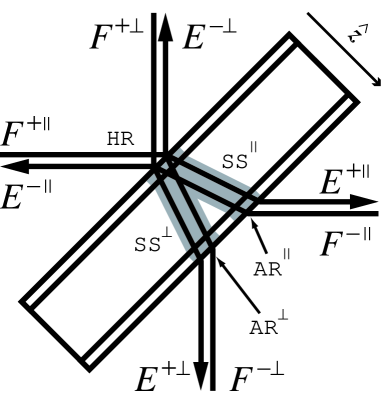
Figure 6: Interaction of the two primary propagation paths — parallel ($\parallel$) and perpendicular ($\perp$) — with the five optical absorption regions that cause thermal focusing in the beamsplitter substrate — SS^∥, SS^⟂, HR, AR^∥, and AR^⟂.

Table 3: Total absorbed TEM₀₀ powers for each of the five absorption regions shown in Fig. 6, summed over the lowest-order transverse modes of all active sidebands. The factors of $\frac{1}{2}$ arise from our normalization convention for the laser electric field.

Region	Absorbed Power
SS∥	$P^{\parallel}_{s}=\alpha_{s}h^{\prime}\,\frac{1}{2}\sum_{q}\left(\left|E^{+\parallel}_{00q}\right|^{2}+\left|F^{-\parallel}_{00q}\right|^{2}\right)$
SS⟂	$P^{\perp}_{s}=\alpha_{s}h^{\prime}\,\frac{1}{2}\sum_{q}\left(\left|E^{+\perp}_{00q}\right|^{2}+\left|F^{-\perp}_{00q}\right|^{2}\right)$
HR	$P_{h}=a_{\mathit{hr}}\,\frac{1}{2}\sum_{q}\biggl{(}\left|F^{+\parallel}_{00q}\right|^{2}+\left|F^{-\parallel}_{00q}\right|^{2}$
	$+\left|F^{+\perp}_{00q}\right|^{2}+\left|F^{-\perp}_{00q}\right|^{2}\biggr{)}$
AR∥	$P^{\parallel}_{a}=a_{\mathit{ar}}\,\frac{1}{2}\sum_{q}\left(\left|E^{+\parallel}_{00q}\right|^{2}+\left|F^{-\parallel}_{00q}\right|^{2}\right)$
AR⟂	$P^{\perp}_{a}=a_{\mathit{ar}}\,\frac{1}{2}\sum_{q}\left(\left|E^{+\perp}_{00q}\right|^{2}+\left|F^{-\perp}_{00q}\right|^{2}\right)$

Diffusion of heat from each of the optical absorption regions contributes to the total OPD distortion for both the parallel and perpendicular propagation paths. Following the conventions we established in Section II.2.2 and Eqs. (31), for the parallel propagation path shown in Fig. 6, we denote the substrate OPD phase operators corresponding to the five absorption regions SS^∥, SS^⟂, HR, AR^∥, and AR^⟂ as $\Phi^{\parallel}_{s}$, $\Phi^{\perp}_{s}$, $\Phi^{\prime}_{c}$, $\Phi^{\parallel}_{c}$, and $\Phi^{\perp}_{c}$, respectively. Since the perpendicular and parallel propagation paths are symmetric under reflection in the $x$-$z$ plane about the $z$ axis, the same set of operators can be used to represent the substrate OPD distortion for perpendicular propagation, but in the order $\Phi^{\perp}_{s}$, $\Phi^{\parallel}_{s}$, $\Phi^{\prime}_{c}$, $\Phi^{\perp}_{c}$, and $\Phi^{\parallel}_{c}$. Hence, in a particular basis, the net substrate thermal OPD matrix operators for the two propagation paths can be written using our unitary approximation as

$$S^{\parallel} = \exp\biggl{\{}i\,\biggl{[}P^{\parallel}_{s}\,\Phi^{\parallel}_{s}+P^{\perp}_{s}\,\Phi^{\perp}_{s}$$ (40a)

$$+P_{h}\,\Phi^{\prime}_{c}+P^{\parallel}_{a}\,\Phi^{\parallel}_{c}+P^{\perp}_{a}\,\Phi^{\perp}_{c}\biggr{]}\biggr{\}},\text{ and}$$

$$S^{\perp} = \exp\biggl{\{}i\,\biggl{[}P^{\parallel}_{s}\,\Phi^{\perp}_{s}+P^{\perp}_{s}\,\Phi^{\parallel}_{s}$$ (40b)

$$+P_{h}\,\Phi^{\prime}_{c}+P^{\parallel}_{a}\,\Phi^{\perp}_{c}+P^{\perp}_{a}\,\Phi^{\parallel}_{c}\biggr{]}\biggr{\}}.$$

For the purposes of the initial LIGO simulations discussed in Section III.5, we first used finite-element software to compute the temperature distribution everywhere in the beamsplitter substrate due to absorption of 1 Watt of TEM₀₀ optical power (choosing the initial LIGO spot size at the beamsplitter) in each of the five regions shown in Fig. 6. Following the same basic approach as that of Section II.2.2, we then computed the matrix elements of the five parallel OPD operators in Eq. (40) using a Hermite-Gauss basis having the same spot size. In our simulation runs, we simply scaled each matrix by the appropriate absorbed power, and then computed $S^{\parallel}$ and $S^{\perp}$ by matrix exponentiation.

II.3.2 Transfer Matrix

As in the case of the mirror described in Section II.2.3, we can construct a generalized transfer matrix for the beamsplitter that includes the effects of aperturing, thermal focusing, and longitudinal microdisplacement. Once again, we adopt the industry-standard convention for the phases of the quarter-wave amplitude reflection and transmission coefficients of the HR coating, and we apply the substrate/AR amplitude transmission coefficient given by Eq. (35) with $h\rightarrow h^{\prime}$. However, as shown in Section II.5.2, the definition of the beamsplitter position is more subtle than that of the mirror: it consists of a static contribution $z$ that represents the location chosen for the beamsplitter when used in cold, unperturbed systems, and a dynamic contribution $\Delta z$ that is used in heated interferometers to maintain a given intracavity phase condition. Hence, if the beamsplitter in Fig. 6 is displaced in the positive $\mathbf{\hat{z}}$ direction (i.e., away from the HR coating along the beamsplitter axis of cylindrical symmetry) by the total displacement $z+\Delta z$, then reflection from the “front” of the beamsplitter introduces an additional relative phase $\exp[+i2\sqrt{2}k(z+\Delta z)]$, while reflection from the “back” of the beamsplitter requires a phase adjustment $\exp[-i2\sqrt{2}k(z+\Delta z)]$.

Collecting these results, the final beamsplitter transfer matrix depicted in Fig. 7 is

$$\begin{bmatrix}E^{-\parallel}\\ E^{+\perp}\\ E^{+\parallel}\\ E^{-\perp}\end{bmatrix}=\begin{bmatrix}T^{-\parallel}&R^{-\parallel}&0&0\\ R^{+\perp}&T^{+\perp}&0&0\\ 0&0&T^{+\parallel}&R^{+\parallel}\\ 0&0&R^{-\perp}&T^{-\perp}\\ \end{bmatrix}\,\begin{bmatrix}F^{-\parallel}\\ F^{+\perp}\\ F^{+\parallel}\\ F^{-\perp}\end{bmatrix},$$ (41)

where, in the absence of curvature mismatch, the transmission operators are

$$T^{-\parallel} = T^{+\parallel}=i\,t\,t^{\prime}_{s}\,S^{\parallel}A,\text{ and}$$ (42a)

$$T^{-\perp} = T^{+\perp}=i\,t\,t^{\prime}_{s}\,S^{\perp}A,$$ (42b)

and the reflection operators are

$$R^{-\parallel} = R^{-\perp}=-r\,e^{+i\,\sqrt{2}k\,(z+\Delta z)}\,A,$$ (43a)

$$R^{+\parallel} = -r\,t_{s}^{\prime\,2}\,e^{-i\,\sqrt{2}k\,(z+\Delta z)}\,S^{\parallel}\,S^{\perp}\,A,\text{ and}$$ (43b)

$$R^{+\perp} = -r\,t_{s}^{\prime\,2}\,e^{-i\,\sqrt{2}k\,(z+\Delta z)}\,S^{\perp}\,S^{\parallel}\,A.$$ (43c)

In the lossless case where $r^{2}+t^{2}=t^{\prime\,2}_{s}=1$ and $A=1$, the explicit unitarity of the $S^{\parallel}$ and $S^{\perp}$ matrix operators guarantees that $|E^{+\perp}|^{2}+|E^{-\parallel}|^{2}=|F^{+\perp}|^{2}+|F^{-\parallel}|^{2}$ and $|E^{+\parallel}|^{2}+|E^{-\perp}|^{2}=|F^{+\parallel}|^{2}+|F^{-\perp}|^{2}$.

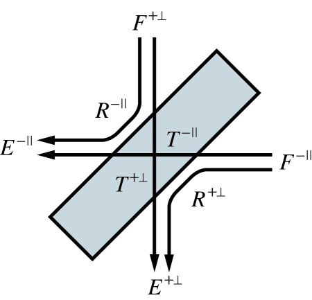
(a) Cross-coupling for $+\perp$ and $-\parallel$

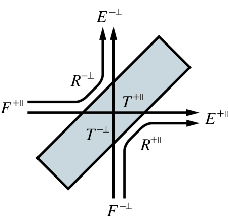
(b) Cross-coupling for $-\perp$ and $+\parallel$

Figure 7: Schematic diagram of the generalized beamsplitter transfer matrix given by Eq. (41). The HR surface of the mirror is on the upper left.

II.4 Fabry-Perot Interferometers

The propagation schematic diagram of a Fabry-Perot interferometer (FPI) is shown in Fig. 8. The front (HR) input and output ports of mirror $\mathcal{M}_{1}$ and $\mathcal{M}_{3}$ are coupled through a propagation distance $L_{13}$. We can simplify later calculations of the optical performance of a power-recycled gravitational-wave interferometer if we first determine a transfer matrix for the FPI, and then establish a procedure maintaining an optimum level of intracavity field amplitude enhancement in the presence of systematic perturbations. Although we develop the FPI transfer matrix in a basis-independent fashion, and postpone the discussion of the choice of an unperturbed basis set until we calculate steady-state fields in Section III.3, we note that we will use the unperturbed Hermite-Gauss eigenmodes of one of the Fabry-Perot interferometers in Fig. 1 to develop a basis set for the entire gravitational-wave detector.

II.4.1 Transfer Matrix

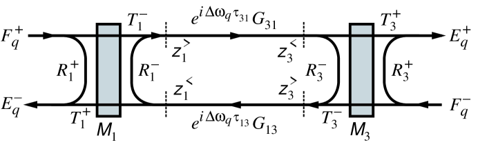
Figure 8: Schematic diagram of the enhancement, reflection, and transmission operators of a Fabry-Perot interferometer, defined by Eq. (50), Eq. (56), and Eq. (55), respectively.

Consider the schematic representation of the enhancement, reflection, and transmission operators of the Fabry-Perot interferometer shown in Fig. 8. If we express these operators using the transfer matrices of mirrors $\mathcal{M}_{1}$ and $\mathcal{M}_{3}$, described in Section II.2.3, then the self-consistent forward propagation steps between the plane of incidence of $\mathcal{M}_{1}$ at $z^{<}_{1}$ and the plane of incidence of $\mathcal{M}_{3}$ at $z^{>}_{3}$ can be represented as

$$F^{-}_{1q} = e^{i\,\Delta\omega_{q}\,\tau_{13}}G_{13}\left(R^{-}_{3}\,F^{+}_{3q}+T^{-}_{3}\,F^{-}_{q}\right),\text{ and}$$ (44a)

$$F^{+}_{3q} = e^{i\,\Delta\omega_{q}\,\tau_{31}}G_{31}\left(R^{-}_{1}\,F^{-}_{1q}+T^{-}_{1}\,F^{+}_{q}\right).$$ (44b)

where $F^{+}_{q}$ is the amplitude of the external sideband field $q$ incident on $\mathcal{M}_{1}$, $F^{-}_{q}$ is the amplitude of the external sideband field $q$ incident on $\mathcal{M}_{3}$, $F^{-}_{1q}$ is the amplitude of frequency component $q$ incident on reference plane $z^{<}_{1}$, and $F^{+}_{3q}$ is the corresponding field incident on reference plane $z^{>}_{3}$. Here $G_{31}$ is the Gouy operator describing the forward propagation step from $z^{>}_{1}$ to $z^{<}_{3}$, while $G_{13}$ is the corresponding operator describing propagation from $z^{>}_{3}$ to $z^{<}_{1}$. (In a power-orthonormal basis, the matrices representing these operators are identical.) If the length of the vacuum separating $\mathcal{M}_{1}$ from $\mathcal{M}_{3}$ is $L_{31}$, then the single-pass propagation time is $\tau_{31}\equiv L_{31}/c=\tau_{13}$.

Using the concatenated column vectors $[E^{-}_{1q}\quad E^{-}_{3q}]^{T}$ and $[F^{-}_{q}\quad F^{+}_{q}]^{T}$, we can construct a system of sparse matrix equations which can be efficiently solved numerically using Gaussian elimination:

$$\left[1-\hat{G}(\Delta\omega_{q})\,\hat{R}^{-}\right]\begin{bmatrix}F^{-}_{1q}\\ F^{+}_{3q}\end{bmatrix}=\hat{G}(\Delta\omega_{q})\,\hat{T}^{-}\,\begin{bmatrix}F^{-}_{q}\\ F^{+}_{q}\end{bmatrix},$$ (45)

where

$$\hat{T}^{-}=\begin{bmatrix}T^{-}_{3}&0\\ 0&T^{-}_{1}\end{bmatrix}\quad\text{ and}\quad\hat{R}^{-}=\begin{bmatrix}0&R^{-}_{3}\\ R^{-}_{1}&0\end{bmatrix}$$ (46)

and

$$\hat{G}(\Delta\omega)=\begin{bmatrix}e^{i\,\Delta\omega\,\tau_{13}}G_{13}&0\\ 0&e^{i\,\Delta\omega\,\tau_{31}}G_{31}\end{bmatrix}.$$ (47)

Alternatively, for a purely analytic calculation, we can define the global enhancement operator

$$\hat{H}(\Delta\omega)=\left[1-\hat{G}(\Delta\omega)\,\hat{R}^{-}\right]^{-1}\hat{G}(\Delta\omega)\,\hat{T}^{-},$$ (48)

and then solve Eq. (45) analytically to obtain

$$\begin{bmatrix}F^{-}_{1q}\\ F^{+}_{3q}\end{bmatrix}=\begin{bmatrix}H^{-}_{1}(\Delta\omega_{q})&H^{+}_{1}(\Delta\omega_{q})\\ H^{-}_{3}(\Delta\omega_{q})&H^{+}_{3}(\Delta\omega_{q})\end{bmatrix}\,\begin{bmatrix}F^{-}_{q}\\ F^{+}_{q}\end{bmatrix},$$ (49)

where the operators representing the enhancements at each of the reference planes in Fig. 8 are given by

$$H^{-}_{1}(\Delta\omega) = \left(1-e^{i\,2\,\Delta\omega\,\tau_{13}}G_{13}\,R^{-}_{3}\,G_{31}\,R^{-}_{1}\right)^{-1}e^{i\,\Delta\omega\,\tau_{13}}G_{13}\,T^{-}_{3},$$ (50a)

$$H^{+}_{1}(\Delta\omega) = \left(1-e^{i\,2\,\Delta\omega\,\tau_{13}}G_{13}\,R^{-}_{3}\,G_{31}\,R^{-}_{1}\right)^{-1}e^{i\,2\,\Delta\omega\,\tau_{13}}G_{13}\,R^{-}_{3}\,G_{31}\,T^{-}_{1},$$ (50b)

$$H^{-}_{3}(\Delta\omega) = \left(1-e^{i\,2\,\Delta\omega\,\tau_{31}}G_{31}\,R^{-}_{1}\,G_{13}\,R^{-}_{3}\right)^{-1}e^{i\,2\,\Delta\omega\,\tau_{31}}G_{31}\,R^{-}_{1}\,G_{13}\,T^{-}_{3},\text{ and}$$ (50c)

$$H^{+}_{3}(\Delta\omega) = \left(1-e^{i\,2\,\Delta\omega\,\tau_{31}}G_{31}\,R^{-}_{1}\,G_{13}\,R^{-}_{3}\right)^{-1}e^{i\,\Delta\omega\,\tau_{31}}G_{31}\,T^{-}_{1}.$$ (50d)

From Fig. 8, we see that each of the output fields $E^{-}_{q}$ and $E^{+}_{q}$ can be expressed as the sum of a prompt reflection of the corresponding input field and an enhanced intracavity field transmitted through the adjacent mirror, giving

$$E^{-}_{q} = T^{+}_{1}\,F^{-}_{1q}+R^{+}_{1}\,F^{+}_{q},\text{ and}$$ (51a)

$$E^{+}_{q} = T^{+}_{3}\,F^{+}_{3q}+R^{+}_{3}\,F^{-}_{q},$$ (51b)

or, from Eq. (48) and Eq. (49),

$$\begin{bmatrix}E^{-}_{q}\\ E^{+}_{q}\end{bmatrix}=\left[\hat{R}^{+}+\hat{T}^{+}\,\hat{H}(\Delta\omega_{q})\right]\,\begin{bmatrix}F^{-}_{q}\\ F^{+}_{q}\end{bmatrix},$$ (52)

where

$$\hat{T}^{+}=\begin{bmatrix}T^{+}_{1}&0\\ 0&T^{+}_{3}\end{bmatrix}\quad\text{ and}\quad\hat{R}^{+}=\begin{bmatrix}0&R^{+}_{1}\\ R^{+}_{3}&0\end{bmatrix}.$$ (53)

We can now construct an explicit transfer matrix similar to Eq. (36) for the FPI as a monolithic optical element. Using Fig. 5 as a guide, Eq. (52) gives:

$$\begin{bmatrix}E^{-}_{q}\\ E^{+}_{q}\end{bmatrix}=\begin{bmatrix}T^{-}_{\text{FPI}}(\Delta\omega_{q})&R^{-}_{\text{FPI}}(\Delta\omega_{q})\\ R^{+}_{\text{FPI}}(\Delta\omega_{q})&T^{+}_{\text{FPI}}(\Delta\omega_{q})\end{bmatrix}\,\begin{bmatrix}F^{-}_{q}\\ F^{+}_{q}\end{bmatrix},$$ (54)

where the transmission operators are

$$T^{-}_{\text{FPI}}(\Delta\omega) = T^{+}_{1}\,H^{-}_{1}(\Delta\omega),\text{ and}$$ (55a)

$$T^{+}_{\text{FPI}}(\Delta\omega) = T^{+}_{3}\,H^{+}_{3}(\Delta\omega),$$ (55b)

and the reflection operators are

$$R^{-}_{\text{FPI}}(\Delta\omega) = R^{+}_{1}+T^{+}_{1}\,H^{+}_{1}(\Delta\omega),\text{ and}$$ (56a)

$$R^{+}_{\text{FPI}}(\Delta\omega) = R^{+}_{3}+T^{+}_{3}\,H^{-}_{3}(\Delta\omega).$$ (56b)

II.4.2 Idealized Simulation of Servo-Controlled Resonator Length Locking

Suppose that the FPI has been initialized using a particular set of configuration parameters for mirrors $\mathcal{M}_{1}$ and $\mathcal{M}_{3}$, the initial thermal loads are negligible, and the initial microdisplacements of both mirrors are set to zero. At some later time, a perturbation is introduced, such as a different curvature for $\mathcal{M}_{1}$, that alters the resonance condition of the cavity. We assume that a biorthonormal set of unperturbed basis functions $u_{mn}({\bf r})$ has been chosen to represent both the intracavity and extracavity transverse laser fields prior to any perturbations, and we wish to compute the corresponding perturbed transfer mirror matrix given by Eq. (36) in that unperturbed basis.

In any experiment using an FPI, the fields emerging from the resonator will be monitored and the cavity length will be adjusted to maintain optimum enhancement. However, rather than simulate a servo-mechanical control loop, we choose to compute a microdisplacement $\Delta z_{1}$ for $\mathcal{M}_{1}$ directly from a numerical determination of the net round-trip phase accumulated by the lowest-loss carrier eigenmode of the resonator. Beginning and ending at the reference plane $z^{<}_{1}$, the perturbed round-trip propagator at the carrier frequency for the FPI shown in Fig. 8 is

$$K_{\text{FPI}}(\Delta z_{1})=e^{-i\,2\,k\,\Delta z_{1}}G_{13}\,R^{-}_{3}\,G_{31}\,R^{-}_{1}$$ (57)

where we have chosen to extract from Eq. (38a) the explicit phase offset arising from a nonzero value of $\Delta z_{1}$.

We can then compute the spectrum of eigenvalues of $K_{\text{FPI}}(0)$, and select the eigenvalue $\lambda_{0}\equiv|\lambda_{0}|e^{i\,\phi_{0}}$ with the largest magnitude (i.e., the smallest round-trip loss). Clearly, the corresponding eigenvector $E_{0}$ is also an eigenvector of the matrix operator $K_{\text{FPI}}(\Delta z_{1})$, with the eigenvalue $\lambda_{1}=\lambda_{0}e^{-i\,2\,k\,\Delta z_{1}}$. Hence, if we choose

$$\Delta z_{1}=\frac{\phi_{0}}{2\,k},$$ (58)

then the net round-trip phase accumulated by $E_{0}$ will be zero, and that mode will satisfy the resonance condition. In our simulations, we maintain a record of the most recently chosen lowest-loss eigenvector, and in the case of degeneracy we choose the eigenmode having the largest value of the inner product with the previous eigenvector.

Suppose that we have followed this procedure and computed the eigenvector $E_{0}$ of the matrix operator $K_{\text{FPI}}(\phi_{0}/2\,k)$, representing a maximally resonant field amplitude at reference plane $z^{<}_{1}$ in Fig. 8. We can mode-match this field by choosing input fields that optimally couple to $E_{0}$ through the global enhancement operator $\hat{H}(0)$. For example, if we solve the matrix equation $E_{0}=H^{+}_{1}(0)\,F^{+}_{0}$ for $F^{+}_{0}$, where $H^{+}_{1}(0)$ is given by Eq. (50b), we obtain the intuitively self-consistent result

$$F^{+}_{0}=\left(\frac{1-\left|\lambda_{0}\right|}{\lambda^{*}_{0}}\right)\,\left(T^{-}_{1}\right)^{-1}R^{-}_{1}\,E_{0}.$$ (59)

A similar mode-matching condition for the back reference plane and incident field can be found using the same procedure.

II.5 Michelson Interferometer

The propagation schematic of a generalized Michelson interferometer (MI) is shown in Fig. 9. The back (AR) parallel input and output ports are coupled to either a mirror or FPI $\mathcal{M}_{\text{I}}$ through a propagation distance $L_{16}$, and the front (HR) perpendicular ports are coupled to either a mirror or FPI $\mathcal{M}_{\text{II}}$ through a propagation distance $L_{26}$. We can simplify later calculations of the optical performance of a power-recycled gravitational wave interferometer if we first determine a transfer matrix for the MI, and then establish a procedure for satisfying the dark port condition in the presence of perturbations. As in Section II.4, we develop the MI transfer matrix in a basis-independent fashion, and postpone the discussion of the choice of an unperturbed basis set until we calculate steady-state fields in Section III.3.

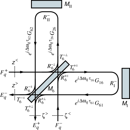
Figure 9: Schematic diagram of the reflection and transmission operators of a Michelson interferometer, defined by Eq. (63). Note that the internal reflection operators $R^{-}_{\text{I}}(\Delta\omega_{q})$ and $R^{-}_{\text{II}}(\Delta\omega_{q})$ may each represent either the reflection operator of a mirror, given by Eq. (38a), or that of a Fabry-Perot interferometer, given by Eq. (56a). The labels $z^{<}$ and $z^{>}$ denote the input and output reference planes, respectively, near the HR surface of the beamsplitter , while $\zeta^{<}$ and $\zeta^{>}$ are the input and output reference planes near the BS AR surface.

II.5.1 Transfer Matrix

By comparing Fig. 7 and Fig. 9, we can connect the MI input and output fields of frequency component $q$ with the front parallel and back perpendicular fields of the beamsplitter using the associations

$$E^{-\parallel} \longrightarrow E^{-}_{q}, \qquad F^{-\perp} \longrightarrow F^{+}_{q}$$

$$E^{+\perp} \longrightarrow E^{+}_{q} \qquad F^{+\parallel} \longrightarrow F^{-}_{q}$$

As shown in Fig. 9, the back parallel fields are coupled through reflection from optical component $\mathcal{M}_{\text{I}}$, and the front perpendicular fields are coupled through reflection from $\mathcal{M}_{\text{II}}$. Therefore, for frequency component $q$, we have

$$F^{-\parallel}_{q} = K_{616}(\Delta\omega_{q})\,E^{+\parallel}_{q},\text{ and}$$ (60a)

$$F^{+\perp}_{q} = K_{626}(\Delta\omega_{q})\,E^{-\perp}_{q}.$$ (60b)

where

$$K_{616}(\Delta\omega) \equiv e^{i\,2\,\Delta\omega\,\tau_{61}}\,G_{61}\,R^{-}_{\text{I}}(\Delta\omega)\,G_{16},\text{ and}$$ (61a)

$$K_{626}(\Delta\omega) \equiv e^{i\,2\,\Delta\omega\,\tau_{62}}\,G_{62}\,R^{-}_{\text{II}}(\Delta\omega)\,G_{26}.$$ (61b)

In Eq. (61a), $G_{16}$ is the Gouy operator describing the forward propagation step from the back parallel output port of the beamsplitter $\mathcal{M}_{6}$ to the input port of $\mathcal{M}_{\text{I}}$, while $G_{61}$ is the corresponding operator describing propagation from the output port of $\mathcal{M}_{\text{I}}$ to the back parallel input port of $\mathcal{M}_{6}$. If the length of the vacuum separating $\mathcal{M}_{6}$ from $\mathcal{M}_{\text{I}}$ is $L_{16}$, then the single-pass propagation time is $\tau_{16}\equiv L_{16}/c=\tau_{61}$. In Eq. (61b), there is an equivalent set of propagation operators and times, with $1\rightarrow 2$ and $\text{I}\rightarrow\text{II}$. The internal reflection operators $R^{-}_{\text{I}}(\Delta\omega)$ and $R^{-}_{\text{II}}(\Delta\omega)$ may each represent either the reflection operator of a mirror, given by Eq. (38a), or that of a Fabry-Perot interferometer, given by Eq. (56a).

By substituting Eq. (60) into Eq. (41), we can immediately construct a transfer matrix similar to Eq. (36) for the MI as a monolithic optical element. Using Fig. 5 as a guide, we find:

$$\begin{bmatrix}E^{-}_{q}\\ E^{+}_{q}\end{bmatrix}=\begin{bmatrix}T^{-}_{\text{MI}}(\Delta\omega_{q})&R^{-}_{\text{MI}}(\Delta\omega_{q})\\ R^{+}_{\text{MI}}(\Delta\omega_{q})&T^{+}_{\text{MI}}(\Delta\omega_{q})\end{bmatrix}\,\begin{bmatrix}F^{-}_{q}\\ F^{+}_{q}\end{bmatrix},$$ (62)

where the individual reflection and transmission operators are defined by the matrix product

$$\begin{split}&\begin{bmatrix}T^{-}_{\text{MI}}(\Delta\omega)&R^{-}_{\text{MI}}(\Delta\omega)\\ R^{+}_{\text{MI}}(\Delta\omega)&T^{+}_{\text{MI}}(\Delta\omega)\end{bmatrix}=\begin{bmatrix}T^{-\parallel}_{6}&R^{-\parallel}_{6}\\ R^{+\perp}_{6}&T^{+\perp}_{6}\end{bmatrix}\\ &\times\,\begin{bmatrix}K_{616}(\Delta\omega)\negthickspace&\negthickspace 0\\ 0\negthickspace&\negthickspace K_{626}(\Delta\omega)\end{bmatrix}\begin{bmatrix}T^{+\parallel}_{6}&R^{+\parallel}_{6}\\ R^{-\perp}_{6}&T^{-\perp}_{6}\end{bmatrix}\begin{bmatrix}0&1\\ 1&0\end{bmatrix}.\end{split}$$ (63)

II.5.2 Idealized Simulation of the Dark Port Condition

Interferometric gravitational-wave Michelson interferometers typically operate with the beamsplitter positioned so that the back perpendicular (antisymmetric) output port generates a dark fringe. In the model MI developed in the previous section, we can adjust the static position $z_{6}$ of the beamsplitter to ensure that an unperturbed, mode-matched fundamental field (i.e., $\{m,n,q\}=\{0,0,0\}$) incident on the beamsplitter’s front parallel input port is cancelled at the back perpendicular output port. Given our conventions for the phases of the amplitude reflection and transmission coefficients of a high-reflectance coating, we choose $z_{6}=-\pi/2\sqrt{2}k$bea99 and obtain from Eq. (43)

$$R^{-\parallel}_{6} = R^{-\perp}_{6}=i\,r_{6}\,e^{+i\,\sqrt{2}k\,\Delta z_{6}}\,A_{6},$$ (64a)

$$R^{+\parallel}_{6} = -i\,r_{6}\,t_{s}^{2}\,e^{-i\,\sqrt{2}k\,\Delta z_{6}}\,S^{\parallel}_{6}\,S^{\perp}_{6}\,A_{6},\text{ and}$$ (64b)

$$R^{+\perp}_{6} = -i\,r_{6}\,t_{s}^{2}\,e^{-i\,\sqrt{2}k\,\Delta z_{6}}\,S^{\perp}_{6}\,S^{\parallel}_{6}\,A_{6}.$$ (64c)

If a compensation plate is placed in the vacuum between the beamsplitter and $\mathcal{M}_{\text{II}}$, then (depending upon its orientation angle) it can be represented as either a mirror or a beamsplitter substrate with two antireflecting coatings and no curvature, and the corresponding operator can be inserted into the perpendicular propagator $K_{626}(\Delta\omega)$ given by Eq. (61b).

Suppose that the MI has been initialized using a particular set of configuration parameters, and in the absence of a thermal lens in any substrate the dynamic microdisplacements of the beamsplitter and the mirrors are set to zero. If the static beamsplitter position has been set to satisfy the dark port condition for $q=0$, then an unperturbed TEM₀₀ field incident on the front parallel port produces a vanishingly small output at the back perpendicular port. Insofar as it is possible, we wish to develop an algorithm that maintains this dark port condition when the system has been perturbed.

Consider an arbitrary field $F^{+}_{0}$ incident on the front input port of the MI. At the back output port, the transmitted field can be found by simplifying Eq. (62) for $q=0$, giving

$$E^{+}_{0}=\left[D_{1}(\Delta z_{6})+D_{2}(\Delta z_{6})\right]\,F^{+}_{0},$$ (65)

where we choose to extract from Eq. (64) the explicit phase offset arising from a nonzero value of $\Delta z_{6}$, and write

$$D_{1}(\Delta z_{6}) = e^{+i\,\sqrt{2}\,k\,\Delta z_{6}}\,R^{+\perp}_{6}\,K_{616}(0)\,T^{+\parallel}_{6},\text{ and}$$ (66a)

$$D_{2}(\Delta z_{6}) = e^{-i\,\sqrt{2}\,k\,\Delta z_{6}}\,T^{+\perp}_{6}\,K_{626}(0)\,R^{-\perp}_{6}.$$ (66b)

The corresponding power measured by a square-law detector at the dark port is therefore (within a constant)

$$\begin{split}P^{+}_{0}(\Delta z_{6})&=\frac{1}{2}\,E^{+{\dagger}}_{0}\,E^{+}_{0}\\ &=\frac{1}{2}\,F^{+{\dagger}}_{0}\,D^{\dagger}_{1}(\Delta\,z_{6})\,D_{2}(\Delta z_{6})\,F_{0}+\text{c.c.}\\ &=\left|F^{+{\dagger}}_{0}\,D^{\dagger}_{1}(0)\,D_{2}(0)\,F_{0}\right|\,\\ &\qquad\times\,\cos\left(2\sqrt{2}\,k\,\Delta z_{6}-\phi\right)\end{split}$$ (67)

where $\phi$ is the phase angle of $-F^{+{\dagger}}_{0}\,D^{\dagger}_{1}(0)\,D_{2}(0)\,F^{+}_{0}$. In order to minimize $P^{+}_{0}(\Delta z_{6})$, we require that the condition $\partial\,P^{+}_{0}(\Delta z_{6})/\partial\,\Delta z_{6}=0$ be satisfied, or

$$\Delta z_{6}=\frac{\phi}{2\sqrt{2}\,k}.$$ (68)

We will incorporate this procedure into a general algorithm for simulating a servo-controlled resonator length-locking system for an entire gravitational-wave interferometer in Section III.2.

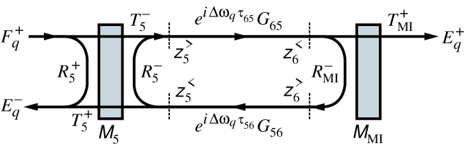
Figure 10: Schematic diagram of the enhancement, reflection, and transmission operators of a power-recycled Fabry-Perot Michelson interferometer, defined by Eq. (70) and Eq. (72), respectively.

III Power-Recycled Fabry-Perot Michelson Interferometer

In previous sections, we have constructed the transfer matrices of the components needed to build a functionally complete description of a power-recycled Fabry-Perot Michelson interferometer (PRFPMI). The PRFPMI propagation schematic shown in Fig. 10 is a simplified form of the FPI schematic displayed in Fig. 8, and will allow us to determine the reduced transfer matrix with a minimum of calculation. In this case, the mirror $\mathcal{M}_{1}$ is replaced by the power-recycling mirror $\mathcal{M}_{5}$, and the mirror $\mathcal{M}_{3}$ is replaced by the Michelson interferometer $\mathcal{M}_{\text{MI}}$. After determining the corresponding enhancement, reflection, and transmission operators of the PRFPMI, we develop a simulation of an idealized servo-controlled length locking system that incorporates the dark port condition algorithm described in Section II.5.2. We then demonstrate the determination of a set of unperturbed basis functions that can be used to describe the electromagnetic intracavity and extracavity fields, and we develop a numerical algorithm for the computation of the steady-state fields under the influence of both geometric and thermal perturbations. After a detailed comparison of the predictions of this model with those of a fast Fourier transform code set in two important special cases, we evaluate the optical performance of the baseline LIGO design.

III.1 Transfer Matrix

Consider the schematic representation of the enhancement, reflection, and transmission operators of the interferometer shown in Fig. 10. If we express these operators using the transfer matrices of $\mathcal{M}_{1}$ and $\mathcal{M}_{\text{MI}}$, respectively described in Section II.2.3 and Section II.5.1, then the intracavity field enhancements can be represented as

$$F^{-}_{5q} = H^{+}_{5}(\Delta\omega_{q})F^{+}_{q},\text{ and}$$ (69a)

$$F^{+}_{6q} = H^{+}_{6}(\Delta\omega_{q})F^{+}_{q}.$$ (69b)

where $F^{+}_{q}$ is the amplitude of the external sideband field $q$ incident on $\mathcal{M}_{5}$, $F^{-}_{5q}$ is the amplitude of frequency component $q$ incident on reference plane $z^{<}_{5}$, and $F^{+}_{6q}$ is the corresponding field incident on reference plane $z^{<}_{6}$. By comparison with Eq. (44), the enhancement operators are

$$H^{+}_{5}(\Delta\omega) = \left[1-e^{i\,2\,\Delta\omega\,\tau_{56}}G_{56}\,R^{-}_{\text{MI}}(\Delta\omega)\,G_{65}\,R^{-}_{5}\right]^{-1}e^{i\,2\,\Delta\omega\,\tau_{56}}G_{56}\,R^{-}_{\text{MI}}(\Delta\omega)\,G_{65}\,T^{-}_{5},$$ (70a)

$$H^{+}_{6}(\Delta\omega) = \left[1-e^{i\,2\,\Delta\omega\,\tau_{65}}G_{65}\,R^{-}_{5}\,G_{56}\,R^{-}_{\text{MI}}(\Delta\omega)\right]^{-1}e^{i\,\Delta\omega\,\tau_{65}}G_{65}\,T^{-}_{5}.$$ (70b)

where $G_{65}$ is the Gouy operator describing the forward propagation step from $z^{>}_{5}$ to $z^{<}_{6}$, and $G_{56}$ is the corresponding operator describing propagation from $z^{>}_{6}$ to $z^{<}_{5}$. If the length of the vacuum separating $\mathcal{M}_{5}$ from $\mathcal{M}_{\text{MI}}$ is $L_{65}$, then the single-pass propagation time is $\tau_{65}\equiv L_{65}/c=\tau_{56}$. The front transmission and reflection operators of the power-recycling mirror, $T^{-}_{5}$ and $R^{-}_{5}$, are given by Eq. (37a) and Eq. (38a), respectively. The front reflection operator of the MI, $R^{-}_{\text{MI}}(\Delta\omega)$, is given by the appropriate element of Eq. (63).

Given the PRFPMI schematic shown in Fig. 10 and the enhancement operators $H^{+}_{5}(\Delta\omega)$ and $H^{+}_{6}(\Delta\omega)$, we obtain the output fields $E^{-}_{q}$ and $E^{+}_{q}$ as

$$E^{-}_{q} = R^{-}_{\text{IFO}}(\Delta\omega_{q})F^{+}_{q},\text{ and}$$ (71a)

$$E^{+}_{q} = T^{+}_{\text{IFO}}(\Delta\omega_{q})F^{+}_{q}.$$ (71b)

where the transmission and reflection operators are

$$T^{+}_{\text{IFO}}(\Delta\omega) = T^{+}_{\text{MI}}(\Delta\omega)\,H^{+}_{6}(\Delta\omega),\text{ and}$$ (72a)

$$R^{-}_{\text{IFO}}(\Delta\omega) = R^{+}_{5}+T^{+}_{5}\,H^{+}_{5}(\Delta\omega).$$ (72b)

III.2 Idealized Simulation of Servo-Controlled Resonator Length Locking

Although the transfer matrix schematics of the FPI and the PRFPMI — shown in Fig. 8 and Fig. 10, respectively — are similar, the resonant structure of the MI and the dark port condition significantly complicate simulations of an idealized resonator length-locking system. Clearly, we need to adjust the position of the power recycling mirror $\mathcal{M}_{5}$ to maintain a “round-trip” resonance condition, but the round trip must include both resonances in the Michelson arms and reflection from a beamsplitter that has been infinitesimally displaced to force compliance with the Michelson dark port condition. In fact, we again choose to compute a microdisplacement $\Delta z_{5}$ for $\mathcal{M}_{5}$ directly from a numerical determination of the net round-trip phase accumulated by the lowest-loss carrier eigenmode of the entire resonator. Beginning and ending at the reference plane $z^{<}_{5}$, the perturbed round-trip propagator at the carrier frequency for the PRFPMI shown in Fig. 10 is

$$\begin{split}K_{\text{IFO}}&(\Delta z_{5},\Delta z_{6})=e^{-i\,2\,k\,\Delta z_{5}}\,\\ &\times G_{56}\biggl{[}T^{-\parallel}_{6}\,K_{616}(0)\,T^{+\parallel}_{6}\\ &+e^{-i\,2\sqrt{2}\,k\,\Delta z_{6}}R^{-\parallel}_{6}\,K_{626}(0)\,R^{-\perp}_{6}\biggr{]}G_{65}\,R^{-}_{5}\end{split}$$ (73)

where we have chosen to extract from Eq. (38a) and Eq. (64a) the explicit phase offsets arising from nonzero values of $\Delta z_{5}$ and $\Delta z_{6}$, respectively.

A close examination of Eq. (73) reveals that we can separate the idealized servo-locking algorithm into three consecutive stages, each with its own optimization process.

1. Follow the procedure described in Section II.4.2 to adjust individually the positions of $\mathcal{M}_{1}$ and $\mathcal{M}_{2}$ to maximize the round-trip enhancement for the lowest-loss carrier eigenmode of each FPI.

2. Select an initial value for $\Delta z_{6}$, and then compute the carrier eigenvalue spectrum of $K_{\text{IFO}}(0,\Delta\,z_{6})$ to find both the eigenvalue $\lambda_{0}$ with the largest magnitude and the corresponding lowest-loss eigenvector $E_{0}$. Set the Michelson input field $F^{+}_{0}=G_{65}\,R^{-}_{5}\,E_{0}$ in Eq. (67), and then use Eq. (68) and the discussion in Section II.5.2 to compute the new beamsplitter position $\Delta z_{6}^{\prime}$ that satisfies the dark port condition for $E_{0}$. Since $E_{0}$ is generally not an eigenvector of $K_{\text{IFO}}(0,\Delta z_{6}^{\prime})$, iterate this step to determine an eigenvector $E^{\prime}_{0}$ and a BS displacement $\Delta z_{6}^{\prime}$ such that successive values of the largest-magnitude eigenvalue $\left|\lambda^{\prime}_{0}\right|$ differ by no more than a suitably small convergence threshold (typically $10^{-12}$ in our simulations).

3. As in the case of the FPI discussed in Section II.4.2, the eigenvector $E^{\prime}_{0}$ is also an eigenvector of the matrix operator $K_{\text{IFO}}(\Delta z_{5},\Delta z^{\prime}_{6})$, with the eigenvalue $\lambda_{5}=\left|\lambda^{\prime}_{0}\right|e^{i\,\left(\phi^{\prime}_{0}-2\,k\,\Delta z_{5}\right)}$. Hence, if we choose

   $$\Delta z_{5}=\frac{\phi^{\prime}_{0}}{2\,k},$$ (74)

   then the net round-trip phase accumulated by $E^{\prime}_{0}$ will be zero, and that mode will satisfy the resonance condition.

As in the case of the FPI, in our simulations we maintain a record of the most recently chosen lowest-loss eigenvector, and in the case of degeneracy we choose the eigenmode having the largest value of the inner product with the previous eigenvector.

Suppose that we have followed this procedure and computed the eigenvector $E^{\prime}_{0}$ of the matrix operator $K_{\text{IFO}}(\phi^{\prime}_{0}/2\,k,\Delta z^{\prime}_{6})$, representing a maximally resonant field amplitude at reference plane $z^{<}_{5}$ in Fig. 10. We can mode-match this field by choosing an input field that optimally couples to $E_{0}$ through the enhancement operator given by Eq. (70a). If we solve the matrix equation $E_{0}=H^{+}_{5}(0)\,F^{+}_{0}$ for $F^{+}_{0}$, we obtain

$$F^{+}_{0}=\left(\frac{1-\left|\lambda_{0}\right|}{\lambda^{*}_{0}}\right)\,\left(T^{-}_{5}\right)^{-1}R^{-}_{5}\,E_{0},$$ (75)

in agreement with Eq. (59).

III.3 Computation of Steady-State Fields

In previous sections, we have been largely unconcerned with the basis chosen to represent the operators which comprise the transfer matrices of the optical elements of the gravitational-wave interferometer. Instead, we have focused on the details of specifying the operator algebra needed to describe the physics of mirror perturbations. In this section, we intend to define a computational algorithm which will allow us to determine the self-consistent steady-state fields everywhere in a realistic model of a thermally loaded interferometer. We begin by describing a procedure to define an unperturbed transverse spatial basis that can be used to represent all intracavity and extracavity electromagnetic fields, and then we specify the initialization process we have used to prepare the computational model for perturbations. Finally, we present the simple iterative steady-state solution algorithm we have used to obtain convergence from the complete set of nonlinear coupled propagation equations describing the PRFPMI intracavity fields.

In the Michelson interferometer, the beamsplitter couples two optical systems (each consisting of a vacuum region followed by either a mirror or a Fabry-Perot interferometer) that may have significantly different mode-matching requirements relative to some common reference plane. In principle, the determination of a set of eigenmodes that is common to both optical systems is a tedious numerical exercise, particularly in the context of the power-recycling scheme shown in Fig. 1. However, in practice, our simulations do not require the identification of an ab initio set of common eigenmodes. Rather, we seek a collection of self-consistent unperturbed basis functions capable of accurately representing the transverse spatial features of the laser field anywhere in the gravitational-wave interferometer. As we show here, these basis functions can be eigenmodes of the unperturbed parallel FPI only, propagated unidirectionally throughout the entire system.

Referring to Fig. 1, Fig. 8, and Fig. 9, we begin by ignoring all apertures everywhere in the system, and choosing the length and mirror curvatures of the unperturbed (e.g., infinite-aperture, spherical-mirror, and cold) parallel FPI. These geometric configuration parameters define a set of standing-wave eigenmodes with a particular spot size and a wavefront radius of curvature at $\mathcal{M}_{1}$ that matches that of $\mathcal{M}_{1}$ prior to thermal loading. We select these eigenmodes as the spatial basis functions that will describe the transverse laser field everywhere in the system.

Referring to Fig. 1 and Fig. 10, we position another mirror at the location of the power recycling mirror (PRM) $\mathcal{M}_{5}$ to couple optically the two Fabry-Perot interferometers, and we propagate the lowest-loss (i.e., “fundamental”) basis function out of the parallel FPI through the beamsplitter to the intracavity input reference plane $z^{<}_{5}$ of the PRM. We calculate the value of the curvature $1/R_{F}$ of the extracted fundamental FPI eigenmode at $z^{<}_{5}$, and set the unperturbed curvature of $\mathcal{M}_{5}$ to that value. We also compute the spot radius $w_{5}$ of the fundamental basis function at $z^{<}_{5}$ so that we can determine the perturbed curvature mismatch matrices $C^{\pm}_{5}$ using the true curvature $1/R_{5}$ in Eq. (14) and Eq. (15).

Following the same unidirectional approach, we propagate the fundamental basis function from the PRM intracavity output reference plane $z^{>}_{5}$ to the intracavity reference planes $z^{>}_{2}$ of $\mathcal{M}_{2}$ and then $z^{>}_{4}$ of $\mathcal{M}_{4}$ in the perpendicular FPI. At each of these two reference planes, we compute the curvature and spot radius of the corresponding laser field, and then set these values as the appropriate unperturbed parameters of these mirrors. As in the case of $\mathcal{M}_{5}$, any discrepancies between the unperturbed curvatures of the propagated basis functions and the true curvatures of the perpendicular mirrors are then captured by the $C^{\pm}$ perturbation matrices defined by Eq. (14).

We complete our specification of the unperturbed geometry of the interferometer by propagating a selected set of unperturbed transverse spatial eigenmodes from the parallel FPI throughout the PRFPMI. This procedure defines a (possibly incomplete) set of spatial basis functions with which intracavity fields in the PRFPMI can be specified. Furthermore, by propagating the intracavity basis functions out through both the dark port and $\mathcal{M}_{5}$, we can use the same unperturbed basis for the extracavity fields $F^{+}$, $E^{+}$, and $E^{-}$ shown in Fig. 10. In general, the input field $F^{+}$ will not be described solely by the outward-propagated fundamental eigenmode of the parallel FPI; instead, it will be represented by a linear combination of some subset of the modes available in the unperturbed basis.

The spherical-mirror, infinite-aperture, cold approximation of the unperturbed gravitational-wave interferometer lends itself to a convenient representation of intracavity fields by power-orthogonal Hermite-Gauss modes. However, even when the mirrors remain spherical and thermal lensing is ignored, this basis cannot represent all possible perturbed fields with arbitrarily high accuracy under all circumstances. For example, in cases where either the recycling cavity is geometrically unstable or a thermal lens is so strong that the sign of the curvature of a wavefront propagating through the substrate changes, then we expect that the number of stable unperturbed basis functions needed to represent that field will become prohibitively large. Furthermore, if either finite apertures or non-spherical mirrors are used to define the unperturbed basis numerically, it is possible that residual diffraction of a non-Hermite-Gauss fundamental basis function from $\mathcal{M}_{5}$ (followed by propagation to $\mathcal{M}_{6}$) will generate a field profile that has a mean spot radius that differs from the value computed using the field profile obtained by propagating the lowest-loss parallel eigenmode from $\mathcal{M}_{1}$ to $\mathcal{M}_{6}$. In this case, a biorthogonal basis can be chosen, but special care must be taken to ensure that the eigenmode expansions converge.kos97 When a self-consistent basis can be chosen, and the corresponding perturbation expansion of the physical observables under simulation converges, the matrix representation of the problem can allow computations which are orders of magnitude faster than those performed by FFT codes.

Now that we have defined a self-consistent set of spatial basis functions at every reference plane in the LIGO PRFPMI, we can introduce the perturbations by setting the apertures and curvatures of the mirrors and beamsplitter to their true values, and then computing the matrices that characterize the effects of aperture diffraction, wavefront-mirror curvature mismatch, and thermal focusing on laser fields expressed as linear combinations of the unperturbed basis functions. Initially, we solve Eq. (69a) in the limit $F^{+}\rightarrow 0$ to obtain the perturbed fields of the cold interferometer, and then we choose a relatively low but finite input power (e.g., 0.1 W) for the input field. The steady-state intracavity fields under this small thermal load can be found using a straightforward, self-consistent procedure:

1. Using the current intracavity fields, compute the powers absorbed in the mirror and beamsplitter substrates and coatings, and update the substrate thermal OPD matrix elements given by Eq. (34) and Eq. (40), which depend nonlinearly on these powers.

2. Following the procedure outlined in Section III.2, adjust the micropositions of $\mathcal{M}_{1}$, $\mathcal{M}_{2}$, $\mathcal{M}_{6}$, and $\mathcal{M}_{5}$ to achieve optimum resonant phase conditions for the lowest-order carrier mode in the each of the three optical cavities.

3. Recompute the intracavity fields using Eq. (69a).

4. Repeat the previous steps until the recycled power $\frac{1}{2}\sum_{q}\left|E^{-}_{5q}\right|^{2}$ has stabilized.

Note that we do not propagate the field from one reference plane to another throughout the interferometer. In this case, even when using the simulated phase control system, the fields tend to converge after a number of iterations implied by the photon storage lifetimes of the arm cavities. Furthermore, we do not use more complicated nonlinear gradient-search methods to determine the intracavity fields because the number of variables (field basis function coefficients) is extremely large, and the variables at any single location in the interferometer is linked to those at all other locations by nontrivial round-trip propagators. Instead, the solution procedure we have detailed above can provide convergence to a few parts in $10^{4}$ in only a few iterations.

The steady-state fields arising from higher input powers can be found by initializing the convergence process with scaled field amplitudes computed at a lower power. For example, if a stable solution has been found at 2 W total input power, then the same collection of intracavity fields, scaled by a factor of two, would be reasonable initial values for an input power of 8 W. Similarly, if the input power is held constant, but some other parameter of the PRFPMI configuration (such as the PRM curvature) is varied, the intracavity fields can be re-used from one parameter value to the next. In this way, a set of solutions for a variety of different interferometer parameter sets can be constructed in a few minutes using a typical desktop computer.

An object-oriented numerical computer model of the initial LIGO interferometer based on these algorithms has been implemented using the class mechanism of the MATLAB programming language.matlab The resulting collection of MATLAB source code files, hereafter referred to as “Melody,” is available publicly for examination and execution.mel01

III.4 Comparison with a Fast Fourier Transform Model

Table 4: High-reflection ($\mathit{hr}$) and anti-reflection ($\mathit{ar}$) loss parameters for the initial LIGO optical elements used in our simulations. Here $a_{c}$ is the optical power absorption that contributes to the substrate thermal loss, and $s_{c}$ is the scattering loss.

	Parameter		Loss (ppm)
	$a_{hr}$			1.0
	$a_{ar}$			1.0
	$s_{hr}$			90.0
	$s_{ar}$			600.0

Table 5: Physical parameters for the initial LIGO optical elements used in our simulations. Each substrate is fused silica, with parameters given by Table 1 and a radius $a=25$ cm. Here the total loss $l_{hr}=a_{hr}+s_{hr}$, where $a_{hr}$ and $s_{hr}$ are the power absorption and scattering losses in the high-reflection coating, respectively.

Mirror	$R_{M}$ (m)	$h$ (m)	$r^{2}$	$t^{2}$
$\mathcal{M}_{1}$, $\mathcal{M}_{2}$	14 571.0	0.10	0.970000	$1-r^{2}-l_{hr}$
$\mathcal{M}_{3}$, $\mathcal{M}_{4}$	7 400.0	0.10	$1-t^{2}-l_{hr}$	$1.5\times 10^{-5}$
$\mathcal{M}_{5}$	9 999.8	0.10	0.985020	$1-r^{2}-l_{hr}$
$\mathcal{M}_{6}$	$\infty$	0.04	0.499975	$1-r^{2}-l_{hr}$

In certain limited cases, the predictions made by Melody can be compared with those of a Fortran implementation of a Fast Fourier Transform (FFT) model of the initial LIGO interferometer.fft98 The FFT model was designed to investigate geometric requirements and tolerances for initial LIGO optical components, and allows either a measured or simulated static OPD phase map to be included in each reflective surface. By contrast, the Melody solution method described in Section III.3 allows the evolving fields everywhere in the interferometer to alter the local phase maps using nonlinear thermal lensing, so that both the field and mirror are distorted by their reciprocal interaction. For the FFT the paraxial approximation is used in order to calculate the propagators between mirrors, as matrix operators in the spatial frequency domain. The lengths are optimized in order to achieve a stationary locked configuration, and the power stored inside the arms and the recycling cavity is evaluated. The final fields obtained may be analyzed for modal composition. In contrast, the Melody program starts with a fixed number of paraxial modes. The matrix elements coupling the modes are then analytically calculated using the algorithms described in Section II.2 and Section II.3, with the thermal effects perturbatively evaluated at every iteration until stationarity is achieved.

While the basic optics and wave-equation assumptions are the same, the two programs have markedly different implementations. In the case of the FFT code, the carrier and the sidebands are simulated by two separate, consecutive runs so that the cavity lengths are optimized for the carrier, and the dimensions of the recycling cavity are optimized for the sidebands. As discussed previously, the idealized Melody control system sets the cavity lengths by ensuring a round trip phase of zero for the lowest-loss eigenmode. The FFT solutions scale linearly with initial field power, but in Melody, the power is shared by carrier and sidebands; the carrier and sideband fields are separately calculated, and their combined power at each iteration affects the thermal lens distortion nonlinearly. The FFT features fine-grained meshing of fixed phase map information, being intended primarily to study arbitrary mirror aberrations. On the other hand, Melody is intended to much more rapidly study coarser-grained effects with specific emphasis on the non-linear effects of thermal focusing. Significantly, the computational hardware requirements for the codes is dramatically different: a typical FFT run requires 30–60 minutes on a supercomputer, while a typical Melody computation requires only a few seconds to stabilize.

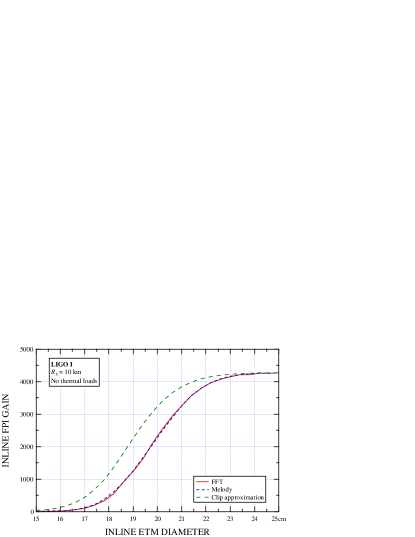
Figure 11: A comparison between the predictions of computer code based on our model (Melody) and those of the FFT model in the case of simple aperturing. The power enhancement (or “gain”) at the parallel/inline FPI reference plane $z^{>}_{1}$ in Fig. 8 is plotted as a function of the aperture of $\mathcal{M}_{3}$. The “clip approximation” represents the result expected by assuming that the loss arises from simple single-pass aperture clipping at $\mathcal{M}_{3}$.

The parameters that we used in our simulations are shown in Table 4 and Table 5. The length of each arm cavity was chosen to be 3999.01 m, and the RF modulation frequency $\omega_{1}/2\pi\equiv 24.493$ MHz (with a modulation depth of 0.44) was adjusted slightly in the Melody computations to guarantee an antiresonance in the arm cavity to within machine precision. The current design value of the initial LIGO common length (the average of the distances between the power recycling mirror and the input test masses) is 9.188 m, and the differential length (or ”Schnupp”) asymmetry (the difference between the distances between the parallel and perpendicular ITM and the PRM) is $L_{S}=0.15$ m. The distance between the beamsplitter and the PRM has the value 6.253 m, and all simulations were performed using the Nd:YAG laser wavelength $\lambda_{0}=1.0642$ $\mu$m. As a first comparison, both codes were used to simulate the unperturbed initial LIGO interferometer, with perfect mode matching, infinite-diameter optics, and no thermal distortion. The agreement between computations of reflected and transmitted power with analytical calculations are within 0.2% for both the FFT code and Melody.

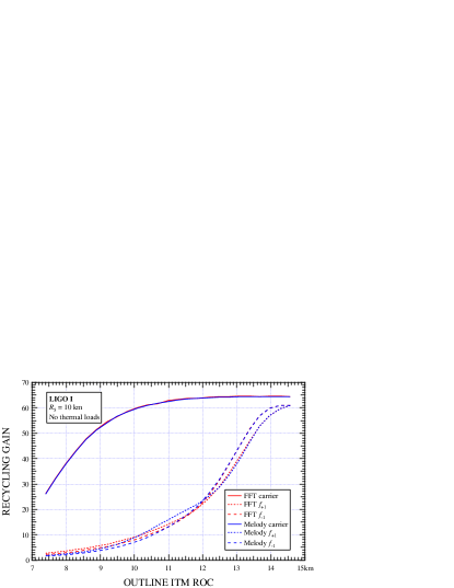
Figure 12: A comparison between the predictions of Melody and those of the FFT model in the case of unstable curvature reduction. The gain at the recycling mirror reference plane $\mathcal{A}^{+}_{5}$ in Fig. 10 is plotted as a function of the curvature of $\mathcal{M}_{2}$. Note that — in the absence of thermal loading — the recycling cavity becomes unstable for the resonant sidebands at a radius of curvature of 14480 m.

In the absence of thermal loading, we have studied the dependence of the parallel (inline) arm cavity power buildup on the diameter of the ETM $\mathcal{M}_{3}$. A comparison between the predictions of Melody and the FFT code tests the suitability of the former’s basis-function-expansion approach to calculating interferometer power levels, particularly when the cavity losses are large enough to require the inclusion of a large number of modes. In Fig. 11, we plot the ratio of the total circulating optical power at reference plane $\mathcal{A}^{+}_{1}$ in Fig. 8 to the total carrier input power $\frac{1}{2}|F^{+}_{0}|^{2}$. When the 28 lowest-loss Hermite-Gauss modes (corresponding to $m+n\leq 6$) of the parallel FPI are used, the agreement is excellent even at an ETM diameter of only 15 cm, which imposes a round-trip diffractive loss of approximately 2000 ppm. For comparison, we have included a trace displaying the stored power in the parallel arm expected when the intracavity loss is due to simple single-pass aperture clipping. Note that this naive assumption underestimates the true diffractive loss by a factor of about 2.14 for this beam spot size at $\mathcal{M}_{3}$.

In the thermally loaded simulations that are described in Section III.5, the increase in thermal focusing power of the ITM substrates improves the geometric stability of the power recycling cavity by increasing the apparent ITM radii of curvatures. However, if we reduce the radius of curvature (ROC) of either ITM below the design value of 14.571 km, the recycling cavity becomes unstable, resulting in a large reduction in stored power. Previous studies of this phenomenon using the FFT code have shown that — for small changes in ITM curvature — only the sidebands suffer this power degradation; the carrier resonance condition in the corresponding arm cavity serves to stabilize the recycling cavity mode by attenuating the anti-resonant higher-order modes. Therefore, since our model uses stable resonator eigenmodes as the spatial basis functions for the field expansions, this is a much more strenuous test than the aperture reduction example, requiring a substantially greater number of transverse modes. In Fig. 12 we show the dependence of the power recycling cavity gain on the perpendicular (outline) ITM radius of curvature. The Melody results for the carrier agree essentially perfectly with those of the FFT code even when we employ only the 28 lowest-loss Hermite-Gauss modes of the parallel FPI. However, to obtain reasonably small discrepancies between the predictions of the sideband behavior in the highly unstable regime, we must include all basis functions satisfying $m+n\leq 20$, or 231 modes.

III.5 Initial LIGO Optical Performance Simulations

We now turn to simulations of the basic initial LIGO interferometer in the presence of thermal loading of the optics. Because of the high power levels maintained in the interferometer to suppress shot noise, the absorption of power in the ITM substrates and coatings and the subsequent thermal focusing must be incorporated into the interferometer design. Using Melody, we explore in detail the effects of this focusing on the optical performance of the interferometer. Since the recycling cavity is operating in a region of geometric stability under full thermal load, we have run our simulations using the 28 lowest-loss Hermite-Gauss modes (corresponding to $m+n\leq 6$) of the parallel FPI.

If the radius of curvature of the power recycling mirror $\mathcal{M}_{5}$ is chosen to be the cold-cavity mode-matched value shown in Table 5, the thermal distortions caused by the substrates in the recycling cavity will destroy this mode-matching and significantly reduce the available recycling gain for the sidebands. In Fig. 13 and Fig. 14, we plot the sideband recycled powers $|F_{5,\pm 1}|^{2}$ given by Eq. (69a) as a function of the PRM ROC $R_{5}$ for the initial LIGO TEM₀₀ operating input laser power of 6.5 W, with 5.9 W delivered by the carrier when the sideband modulation depth is 0.44. The presence of the arm cavities significantly reduces the sensitivity of the carrier to these perturbations, resulting in an approximately constant recycling gain of 30 when the parameters specified in Table 1, Table 5, and Table 4 are used. Note that the optimum mode-matching of the parallel and perpendicular segments of the recycling cavity occurs when the PRM ROC has increased to approximately 15 km.

One of the most striking details of Fig. 13 and Fig. 14 is the significant difference in the recycling gain of the upper ($+\Delta\omega_{1}$) and lower ($-\Delta\omega_{1}$) sideband fields. Such a sideband imbalance can lead to significant gravitational-wave detection noise signatures that are qualitatively absent when the balance is exact. Since the ratio $\Delta\omega_{1}/\omega_{0}$ is immeasurably small for RF sidebands and (by design) there is a very high degree of geometrical symmetry between the Michelson branches of the interferometer, we naively expect the sideband fields to interact identically with geometrical distortions as long as these distortions are frequency-independent at the RF scale. In principle, this symmetry is broken only by the macroscopic value of the Schnupp asymmetry $L_{S}\equiv L_{51}-L_{52}$, where $L_{5j}$ is the optical path length separating the $\mathcal{M}_{5}$ and $\mathcal{M}_{j}$. For gravitational-wave interferometers, $L_{S}$ is much smaller than the Rayleigh length, so both sidebands should interact nearly identically with either arm, except for a phase accumulation proportional to the distortion-independent factor $\Delta\omega_{1}L_{S}$. Using both Melody and the FFT code, we have determined that our simulations strictly show excellent sideband balance if either $L_{S}\rightarrow 0$ or the net branch distortions are identical. However, with Melody we have determined that the branch distortions cannot be identical when the thermal lens in the beamsplitter substrate is significant; this source of additional distortion in the parallel arm requires a significant displacement of the beamsplitter to maintain the dark port condition, and is therefore the primary cause of the imbalance shown in Fig. 13 and Fig. 14. In fact, as seen in Fig. 12, the FFT code reproduces this behavior when the field-mirror curvature mismatch at the perpendicular ITM becomes large, causing a significant difference between the net distortions of the two arms. Further studies using Melody have shown that it is possible to improve the sideband balance by supplementing the procedure outlined in Section III.2 with an additional step that readjusts the positions of both $\mathcal{M}_{5}$ and $\mathcal{M}_{6}$, at the expense of increasing the TEM₀₀ carrier output power.

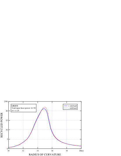
Figure 13: Initial LIGO recycled powers as a function of the PRM radius of curvature. The total TEM₀₀ input laser power is 6.5 W, with 5.9 W delivered by the carrier.

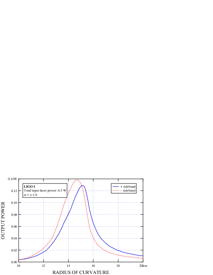
Figure 14: Initial LIGO dark port powers as a function of the PRM radius of curvature. The total TEM₀₀ input laser power is 6.5 W, with 5.9 W delivered by the carrier.

For the purposes of our discussion here, we have chosen a value of the PRM ROC that minimizes both the fundamental carrier power and the sideband imbalance at the output port. This strategy produces the optimum initial LIGO PRM radius of curvature as a function of total TEM₀₀ input laser power shown in Fig. 15. Again, we have assumed a modulation depth of 0.44, which pushes about 10% of the total available laser power into the sidebands. The corresponding optimized initial LIGO recycled and output sideband powers are shown in Fig. 16 and Fig. 17, respectively. Note that at each value of the input power in these two plots, the corresponding PRM ROC shown in Fig. 15 has been used. Although the residual imbalance of the recycled sideband fields remains at the 10% level at an input power of 10 W, the imbalance at the antisymmetric port is negligible.

As an example of the operating characteristics of a fixed interferometer design point, Fig. 18 and Fig. 19 give the recycled and output powers at the carrier and sideband modulation frequencies for an interferometer optimized for a total laser input power of 6.5 W. The optimum PRM ROC is 15.075 km, and, as shown in Fig. 18, the recycling gain for the carrier is about 30. Figure 19 predicts that, at 6.5 W, the sidebands are approximately balanced, with about 130 mW in each field, while the total carrier power emerging from the dark port is about 180 $\mu$W. Approximately 90% of this carrier power is stored in higher-order modes.

The behavior of the idealized PRFPMI phase-control system is illustrated in Fig. 20. The PRM ($\mathcal{M}_{5}$) is initially pulled in toward the beamsplitter to compensate for the longitudinal phase introduced by the mismatch between the curvatures of the field emerging from the parallel FPI and the PRM itself. However, as the strengths of the thermal lenses in the ITM substrates increase, the mirror is pushed away from the beamsplitter to maintain the carrier resonance. Similarly, as the astigmatic thermal lens develops in the beamsplitter substrate, the beamsplitter moves slightly toward the upper left in Fig. 1. Indeed, as we see in Fig. 21, even in the $y$ plane the effective focal length of the beamsplitter substrate is six times larger than that of either ITM substrate; nevertheless, the resulting asymmetry between the two Michelson arms is numerically detected and compensated.

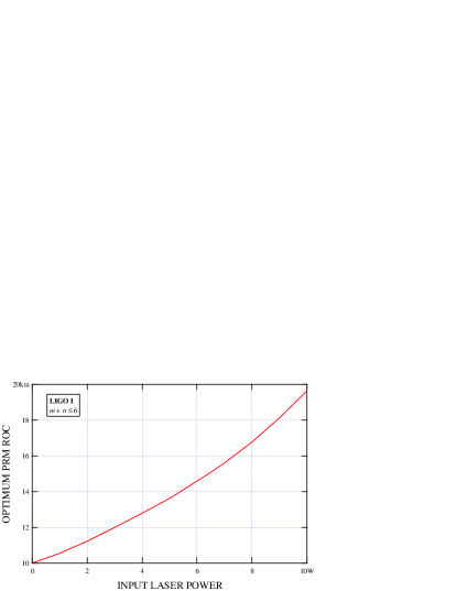
Figure 15: The optimum initial LIGO PRM radius of curvature as a function of total TEM₀₀ input laser power.

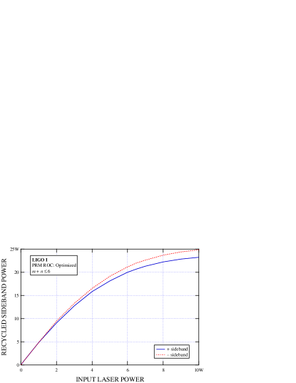
Figure 16: Optimized initial LIGO recycled sideband powers as a function of total TEM₀₀ input laser power. At each value of the input power, the PRM radius of curvature shown in Fig. 15 has been used.

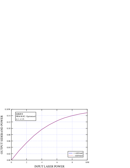
Figure 17: Optimized initial LIGO output sideband powers as a function of total TEM₀₀ input laser power. At each value of the input power, the PRM radius of curvature shown in Fig. 15 has been used.

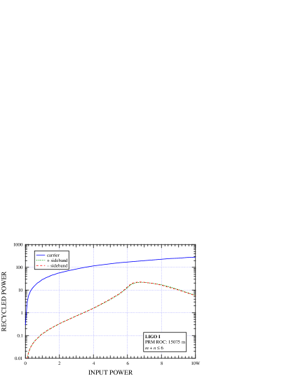
Figure 18: Initial LIGO recycled powers as a function of total TEM₀₀ input laser power. The PRM radius of curvature is 15075 m, the optimized value for an input power of 6.5 W.

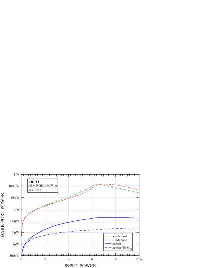
Figure 19: Initial LIGO dark port powers as a function of total TEM₀₀ input laser power.

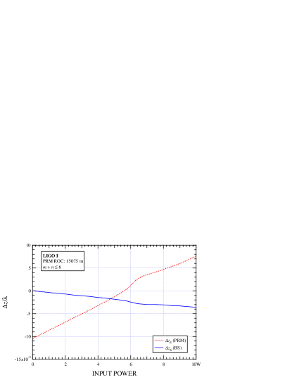
Figure 20: Initial LIGO PRM and BS microdisplacements as a function of total TEM₀₀ input laser power.

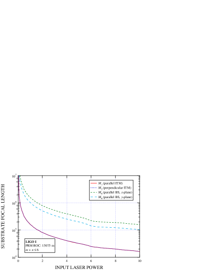
Figure 21: Initial LIGO effective (i.e., quadratic) thermal focal lengths as a function of total TEM₀₀ input laser power.

IV Conclusion

We have developed highly detailed steady-state analytical and numerical models of the physical phenomena which limit the intracavity power enhancement of recycled Michelson Fabry-Perot laser gravitational-wave detectors. We have included in our operator-based formalism the effects of nonlinear thermal lensing due to power absorption in both the substrates and coatings of the mirrors and beamsplitter, the effects of any mismatch between the curvatures of the laser wavefront and the mirror surface, and the diffraction by an aperture at each instance of reflection and transmission. We have taken great care to preserve numerically the nearly ideal longitudinal phase resonance conditions that would otherwise be provided by an external servo-locking control system. Once the mirrors and beamsplitters have been analyzed and their transfer matrices constructed, more complicated optical components and structures (such as Fabry-Perot and Michelson interferometers, and the LIGO detector) can be modeled using simple matrix composition.

Our formalism relies on the validity of an expansion of the intracavity electromagnetic field at any reference plane in a necessarily incomplete set of possibly biorthogonal basis functions that are derived from eigenmodes of one of the Fabry-Perot arm cavities. In two specific cases, we have checked the results produced by Melody — a fast MATLAB implementation of our model — against those generated by an FFT program used to model optical imperfections in LIGO. We have found that Melody can accurately predict the behavior of the carrier even in highly perturbed cold resonators using a modest number of spatial basis functions in orders of magnitude less time than is required by the FFT code. The same is true for the sideband fields stored in the power recycling cavity, except in the case where the recycling cavity is significantly geometrically unstable. Even in this situation (which does not arise when the interferometer is thermally loaded), accuracy can be improved substantially by including more modes in the simulation.

We have discovered and described in broad terms the conditions under which the power stored in the two sideband fields can become unbalanced, potentially affecting the noise sensitivity of the gravitational-wave interferometer in the detection band. At this point, we believe that an additional post-process step can be introduced into our simulated phase-locking algorithm that will allow a reduction of the sideband imbalance at the expense of a previously optimized optical property of the carrier field.

In the future, we will include the effects of thermoelastic surface deformation in our model, and apply it to proposed configurations of the advanced LIGO interferometer. Other systematic perturbations and imperfections (e.g., mirror tilt and substrate inhomogeneities) can be included easily by incorporating the appropriate operators into the transfer matrices describing reflection and transmission for the mirrors and beamsplitter. In addition, we intend to develop algorithms for the simulation of the optical response of an interferometer to gravitational radiation, with the intention of estimating the detection sensitivity of advanced LIGO under full thermal load. We anticipate that the performance of the Melody program will not be significantly affected by these modifications.

- (1) C. M. Will, Theory and Experiment in Gravitational Physics, rev. ed. (Cambridge University Press, Cambridge, 1993).
- (2) D. G. Blair, ed.,The Detection of Gravitational Waves (Cambridge University Press, Cambridge, 1993).
- (3) P. R. Saulson, Fundamentals of Interferometric Gravitational Wave Detectors (World Scientific, Singapore, 1994).
- (4) A. Abramovici, W. Althouse, R. Drever, Y. Gursel, S. Kawamura, F. Raab, D. Shoemaker, L. Sievers, R. Spero, K. Thorne, R. Vogt, R. Weiss, S. Whitcomb, and M. Zucker, “LIGO: The Laser Interferometer Gravitational-Wave Observatory,” Science 256, 325–333 (1992).
- (5) A. Abramovici, W. Althouse, J. Camp, J. A. Giaime, A. Gillespie, S. Kawamura, A. Kuhnert, T. Lyons, F. J. Raab, R. L. Savage Jr., D. Shoemaker, L. Sievers, R. Spero, R. Vogt, R. Weiss, S. Whitcomb, and M. Zucker, “Improved sensitivity in a gravitational wave interferometer and implications for LIGO,” Phys. Lett. A 218, 157–163 (1996).
- (6) A. Giazotto, “The VIRGO experiment: status of the art,” in First Edoardo Amaldi Conference on Gravitational Wave Experiments, E. Coccia, G. Pizella and F. Ronga (eds.), (World Scientific, Singapore, 1995), p. 86.
- (7) K. Danzmann, “GEO 600—A 600-m Laser Interferometric Gravitational Wave Antenna,” in First Edoardo Amaldi Conference on Gravitational Wave Experiments, E. Coccia, G. Pizella and F. Ronga (eds.), (World Scientific, Singapore, 1995), p. 100.
- (8) K. Tsubono, “300-m Laser Interferometric Gravitational Wave Detector (TAMA300) in Japan,” in First Edoardo Amaldi Conference on Gravitational Wave Experiments, E. Coccia, G. Pizella and F. Ronga (eds.), (World Scientific, Singapore, 1995), p. 112.
- (9) R. W. P. Drever, J. L. Hall, F. V. Kowalski, J. Hough, G. M. Ford, A. J. Munley, H. Ward, “Laser phase and frequency stabilization using an optical resonator,” Appl. Phys. B 31, 97–105 (1983).
- (10) P. Fritschel, R. Bork, G. Lez, N. Mavalvala, D. Ouimette, H. Rong, D. Sigg, M. Zucker, “Readout and control of a power-recycled interferometric gravitational-wave antenna,” Appl. Opt.-OT 40, 4988–4998 (2001).
- (11) B. J. Meers and K. A. Strain, “Wave-front distortion in laser-interferometric gravitational-wave detectors,” Phys. Rev. D 43, 3117–3130 (1991).
- (12) W. Winkler, K. Danzmann, A. Rüdiger, and R. Schilling, “Heating by optical absorption and the performance of interfeometric gravitational-wave detectors,” Phys. Rev. A 44, 7022–7036 (1991).
- (13) K. A. Strain, K. Danzmann, J. Mizuno, P. G. Nelson, A. Rüdiger, R. Schilling, W. Winkler, “Thermal lensing in recycling interferometric gravitational wave detectors,” Phys. Lett. A 194, 124–132 (1994).
- (14) D. McClelland, J. Camp, J. Mason, W. Kells, S. Whitcomb, “Arm cavity resonant sideband control for laser interferometric gravitational wave detectors,” Opt. Lett. 24, 1014–1016 (1999).
- (15) J.-Y. Vinet, P. Hello, C. N. Man, and A. Brillet, “A high-accuracy method for the simulation of non-ideal optical cavities,” J. Phys. (Paris) I 2, 1287–1303 (1992).
- (16) P. Saha, “Fast estimation of transverse fields in high-finesse optical cavities,” J. Opt. Soc. Am. A14, 2195–2202 (1997).
- (17) B. Bochner, “Modeling the performance of interferometric gravitational-wave detectors with realistically imperfect optics,” Ph.D. thesis (Massachusetts Institute of Technology, Cambridge, MA, 1998).
- (18) P. Hello and J.-Y. Vinet, “Analytical models of thermal aberrations in massive mirrors heated by high power laser beams,” J. Phys. France 51, 1267–1282 (1990).
- (19) D. Z. Anderson, “Alignment of resonant optical cavities,” Appl. Opt. 23, 2944–2949 (1984).
- (20) E. Morrison, B. J. Meers, D. I. Robertson, and H. Ward, “Automatic alignment of optical interferometers,” Appl. Opt. 33, 5041–5049 (1994).
- (21) Y. Hefetz, N. Mavalvala, and D. Sigg, “Principles of calculating alignment signals in complex resonant optical interferometers,” J. Opt. Soc. Am. B 107, 1597–1605 (1997).
- (22) R. G. Beausoleil and D. Sigg, “Spatiotemporal model of the LIGO interferometer,” J. Opt. Soc. Am. A 16, 2990–3002 (1999).
- (23) A. E. Siegman, Lasers (University Science, Mill Valley, 1986); errata URL: http://www-ee.stanford.edu/∼siegman/lasers_book_errata.txt.
- (24) K. E. Oughstun, in Progress in Optics, E. Wolf, ed. (North-Holland, Amsterdam, 1987), Vol. 24, pp. 165–387.
- (25) A. Kostenbauder, Y. Sun, and A. E. Siegman, “Eigenmode expansions using biorthogonal functions: complex-valued Hermite-Gaussians,” J. Opt. Soc. A 14, 1780–1790 (1997).
- (26) See http://www.mathworks.com/products/matlab/.
- (27) The Melody/MATLAB software package can be downloaded from the LIGO Software Tools for Advanced Interferometer Configurations Internet web site at the URL http://www.phys.ufl.edu/LIGO/LIGO/STAIC.html.