WATPHYS-TH01/06

Particles on a Circle in Canonical Lineal Gravity

R.B. Mann

Dept. of Physics, University of Waterloo Waterloo, ONT N2L 3G1, Canada

PACS numbers: 04.20.C, 04.60.K, 04.80.+z

A description of the canonical formulation of lineal gravity minimally coupled to N point particles in a circular topology is given. The Hamiltonian is found to be equal to the time-rate of change of the extrinsic curvature multiplied by the proper circumference of the circle. Exact solutions for pure gravity and for gravity coupled to a single particle are obtained. The presence of a single particle significantly modifies the spacetime evolution by either slowing down or reversing the cosmological expansion of the circle, depending upon the choice of parameters.

1 INTRODUCTION

An increasing amount of attention is being given to the problem of lower-dimensional self-gravitating systems.  These systems consist of a collection of $\ N$ particles mutually interacting through their own mutual gravitational attraction, along with other specified forces.  They are used not only as prototypes for the behaviour of gravity in higher dimensions, but can also also approximate the behaviour of some physical systems in 3 spatial dimensions, such as the dynamics of stars in a direction orthogonal to the plane of a highly flattened galaxy, the collisions of flat parallel domain walls, and the dynamics of cosmic strings. For the many-body case there has been much work on understanding the fractal behaviour [1] and ergodic and equipartition properties [2] of non-relativistic one-dimensional self-gravitating systems. Only recently has this been extended to included relativistic effects [3].  For the 2-body case there is an exact relativistic solution in 2 spatial dimensions [4], although it does not have a non-relativistic limit. Several exact solutions to the 2-body problem have been found in one spatial dimension [6]. These have a non-relativistic limit  [5], and have been extended to include both cosmological expansion [7, 8] and electromagnetic interactions [9]. All solutions obtained so far have been for non-compact spatial dimensions.

The purpose of this paper is to extend to circular topology the $N$-body problem for relativistic gravity in $(1+1)$ dimensions (i.e. lineal gravity).  This is the only compact topology available in one spatial dimension and it introduces qualitatively new features not present in the non-compact case. For example, an analogous non-relativistic solution does not exist (as is the case in higher dimensions).  This is easily seen by considering the non-relativistic canonical field equations for a point source in one spatial dimension

$$\varphi^{\prime\prime} = m\;\delta(x-z(t))\;$$ (1)

$$\dot{p} = -\varphi^{\prime}\left(z\right)$$ (2)

$$\dot{z_{a}} = \frac{p}{m}$$ (3)

where the prime refers to the derivative with respect to the spatial coordinate $x$. The first equation yields a solution for the gravitational potential $\varphi$ which grows linearly with $x$.  This is consistent with the remaining equations, taking $p=z=0$ and $\varphi=\frac{m}{2}\left|x\right|$, which has vanishing derivative at the origin. For a lineal topology this is fine, but for a circular topology we must have both $\varphi(L)=\varphi(-L)$ and  $\varphi^{\prime}(L)=\varphi^{\prime}(-L)$ for some $L$, where $2L$ is the circumference of the circle. There is no solution to these matching conditions unless another point source of negative mass is introduced.   For any compact smeared source the problem is the same: the potential grows linearly with increasing distance from the source and the matching conditions cannot be satisfied for physically reasonable (i.e. positive mass) sources.  However in a dynamical spacetime this problem has a solution since the spacetime can expand or contract in response to the presence of the source.

In this paper I formulate a general framework for canonical reduction of lineal gravity minimally coupled to $N$ particles in the presence of a cosmological constant $\Lambda$.  This extends previous work done in the non-compact case [5] and is somewhat analogous to the reduction of the $(2+1)$ dimensional Einstein equations for spatially compact manifolds to a Hamiltonian system [11].  Choosing the mean curvature to play the role of time, I find that the Hamiltonian becomes the circumference functional of the circle.  After establishing the basic formalism, I solve the canonical equations for $N=0$ (pure gravity) and $N=1$.

The lineal gravity theory chosen here is one that models 4D general relativity in that it sets the Ricci scalar equal to the trace of the stress-energy of prescribed matter fields and sources. This theory (sometimes referred to as $R=T$ theory) has the property that matter governs the evolution of spacetime curvature which reciprocally governs the evolution of matter [12]. It has a consistent Newtonian limit [12], a problematic limit in a generic $(1+1)$-dimensional theory of gravity theory [13]. Setting the particle stress-energy to zero, leaving only the cosmological constant, the theory reduces to Jackiw-Teitelboim (JT) theory [14].  Since pure gravity in $(1+1)$-dimensions has no dynamics (the Einstein-Hilbert action is a topological invariant) it is necessary to include a scalar (dilaton) field in the action [15].  The particular choice of dilaton coupling in $R=T$ theory is such that the evolution of the dilaton does not modify the reciprocal gravity/matter dynamics noted above.

The outline of the paper is as follows. In section 2 the canonical formulation of the $N$-particle self-gravitating system in $(1+1)$ dimensions is given, and the Hamiltonian is shown to be proportional to the circumference functional of the circle multiplied by the time-rate-of-change of the extrinsic curvature. In section 3 the equations are solved in the pure gravity case with cosmological constant using two different methods.  In section 4 the equations are solved in the single particle case, and then analyzed using a variety of different choices for the time dependence of the extrinsic curvature. The last section contains a summary of the work and some suggestions for further research.

2 CANONICAL REDUCTION OF THE $N$-PARTICLE SYSTEM

The canonical reduction of  the $N$-body problem in $(1+1)$-dimensions with circular topology has several features in common with that of its non-compact counterpart [5, 6, 8].  The action integral for the gravitational fields coupled with $N$ point masses is

$$I = \int d^{2}x\left[\frac{1}{2\kappa}\sqrt{-g}g^{\mu\nu}\left\{\Psi R_{\mu\nu}+\frac{1}{2}\nabla_{\mu}\Psi\nabla_{\nu}\Psi+\frac{1}{2}g_{\mu\nu}\Lambda\right\}\right.$$ (4)

$$\qquad\left.+\sum_{a}\int d\tau_{a}\left\{-m_{a}\left(-g_{\mu\nu}(x)\frac{dz_{a}^{\mu}}{d\tau_{a}}\frac{dz_{a}^{\nu}}{d\tau_{a}}\right)^{1/2}\right\}\delta^{2}(x-z_{a}(\tau_{a}))\right]\;,$$

where $\Psi$ is the dilaton field, $g_{\mu\nu}$ and $g$ are the metric and its determinant, $R$ is the Ricci scalar, and $e_{a}$ and $\tau_{a}$ are the charge and the proper time of $a$-th particle, respectively, with $\kappa=8\pi G/c^{4}$. The symbol $\nabla_{\mu}$ denotes the covariant derivative associated with $g_{\mu\nu}$. Here I take the range of $x$ to be $-L\leq x\leq L$, and the circular topology implies that all fields must be smooth (or at least $C^{1}$) functions of $x$ with period $2L$, which implies

$$f(L)=f(-L)\qquad\text{and}\qquad f^{\prime}(L)=f^{\prime}(-L)=0\;\;.$$ (5)

for all functions.

The field equations derived from the action (4) are

$$R-g^{\mu\nu}\nabla_{\mu}\nabla_{\nu}\Psi=0\;,$$ (6)

$$\frac{1}{2}\nabla_{\mu}\Psi\nabla_{\nu}\Psi-\frac{1}{4}g_{\mu\nu}\nabla^{\lambda}\Psi\nabla_{\lambda}\Psi+g_{\mu\nu}\nabla^{\lambda}\nabla_{\lambda}\Psi-\nabla_{\mu}\nabla_{\nu}\Psi=\kappa T_{\mu\nu}+\frac{1}{2}g_{\mu\nu}\Lambda\;,$$ (7)

$$m_{a}\left[\frac{d}{d\tau_{a}}\left\{g_{\mu\nu}(z_{a})\frac{dz_{a}^{\nu}}{d\tau_{a}}\right\}-\frac{1}{2}g_{\nu\lambda,\mu}(z_{a})\frac{dz_{a}^{\nu}}{d\tau_{a}}\frac{dz_{a}^{\lambda}}{d\tau_{a}}\right]=0\;,$$ (8)

where

$$T_{\mu\nu}=\sum_{a}m_{a}\int d\tau_{a}\frac{1}{\sqrt{-g}}g_{\mu\sigma}g_{\nu\rho}\frac{dz_{a}^{\sigma}}{d\tau_{a}}\frac{dz_{a}^{\rho}}{d\tau_{a}}\delta^{2}(x-z_{a}(\tau_{a}))\;,$$ (9)

is the stress-energy due to the point masses. Conservation of $T_{\mu\nu}$ is ensured by eq.(7). Note that insertion of the trace of eq.(7) into (6) yields

$$R-\Lambda=\kappa T_{\;\;\mu}^{\mu}\;.$$ (10)

Eqs. (8) and (10) form a closed sytem of equations for gravity and matter.

To canonically reduce this system, write the metric in the form

$$ds^{2}=-N_{0}^{2}dt^{2}+\gamma\left(dx+\frac{N_{1}}{\gamma}dt\right)^{2}\;,$$ (11)

so that $\gamma=g_{11},N_{0}=(-g^{00})^{-1/2}$ and $N_{1}=g_{10}$.  Decomposing the scalar curvature in terms of the extrinsic curvature $K$ via

$$\sqrt{-g}R=-2\partial_{0}(\sqrt{\gamma}K)+2\partial_{1}[(N_{1}K-\partial_{1}N_{0})/\sqrt{\gamma}]\;,$$ (12)

where

$$K=(2N_{0}\gamma)^{-1}(2\partial_{1}N_{1}-\gamma^{-1}N_{1}\partial_{1}\gamma-\partial_{0}\gamma)$$ (13)

yields for the action (4)

$$I=\int d^{2}x\left\{\sum_{a}p_{a}\dot{z}_{a}\delta(x-z_{a}(t))+\pi\dot{\gamma}+\Pi\dot{\Psi}+N_{0}R^{0}+N_{1}R^{1}\right\}$$ (14)

where $\pi$ and $\Pi$ are conjugate momenta to $\gamma$ and $\Psi$, respectively and $p_{a}$ is the momentum conjugate to the coordinate $z_{a}$. The constraints are

$$R^{0} = -\kappa\sqrt{\gamma}\gamma\pi^{2}+2\kappa\sqrt{\gamma}\pi\Pi+\frac{1}{4\kappa\sqrt{\gamma}}(\Psi^{\prime})^{2}-\frac{1}{\kappa}\left(\frac{\Psi^{\prime}}{\sqrt{\gamma}}\right)^{\prime}-\frac{1}{2}\sqrt{\gamma}(-\frac{\Lambda}{\kappa})$$ (15)

$$-\sum_{a}\sqrt{\frac{p_{a}^{2}}{\gamma}+m_{a}^{2}}\;\delta(x-z_{a}(t))\;,$$

$$R^{1} = \frac{\gamma^{\prime}}{\gamma}\pi-\frac{1}{\gamma}\Pi\Psi^{\prime}+2\pi^{\prime}+\sum_{a}\frac{p_{a}}{\gamma}\delta(x-z_{a}(t))\;,$$ (16)

with the symbols $(\;\dot{}\;)$ and $(\;^{\prime}\;)$ denoting $\partial_{0}$ and $\partial_{1}$, respectively.

From the action (14) the set of field equations is

$$\dot{\pi} + N_{0}\left\{\frac{3\kappa}{2}\sqrt{\gamma}\pi^{2}-\frac{\kappa}{\sqrt{\gamma}}\pi\Pi+\frac{1}{8\kappa\sqrt{\gamma}\gamma}(\Psi^{\prime})^{2}-\frac{1}{4\sqrt{\gamma}}\frac{\Lambda}{\kappa}\right.$$ (17)

$$\makebox[100.00015pt]{}\left.-\sum_{a}\frac{p_{a}^{2}}{2\gamma^{2}\sqrt{\frac{p_{a}^{2}}{\gamma}+m_{a}^{2}}}\;\delta(x-z_{a}(t))\right\}$$

$$+ N_{1}\left\{-\frac{1}{\gamma^{2}}\Pi\Psi^{\prime}+\frac{\pi^{\prime}}{\gamma}+\sum_{a}\frac{p_{a}}{\gamma^{2}}\;\delta(x-z_{a}(t))\right\}+N_{0}^{\prime}\frac{1}{2\kappa\sqrt{\gamma}\gamma}\Psi^{\prime}+N_{1}^{\prime}\frac{\pi}{\gamma}=0\;,$$

$$\dot{\gamma}-N_{0}(2\kappa\sqrt{\gamma}\gamma\pi-2\kappa\sqrt{\gamma}\Pi)+N_{1}\frac{\gamma^{\prime}}{\gamma}-2N_{1}^{\prime}=0\;,$$ (18)

$$R^{0}=0\;,$$ (19)

$$R^{1}=0\;,$$ (20)

$$\dot{\Pi}+\partial_{1}(-\frac{1}{\gamma}N_{1}\Pi+\frac{1}{2\kappa\sqrt{\gamma}}N_{0}\Psi^{\prime}+\frac{1}{\kappa\sqrt{\gamma}}N_{0}^{\prime})=0\;,$$ (21)

$$\dot{\Psi}+N_{0}(2\kappa\sqrt{\gamma}\pi)-N_{1}(\frac{1}{\gamma}\Psi^{\prime})=0\;,$$ (22)

$$\dot{p}_{a}+\frac{\partial N_{0}}{\partial z_{a}}\sqrt{\frac{p_{a}^{2}}{\gamma}+m_{a}^{2}}-\frac{N_{0}}{2\sqrt{\frac{p_{a}^{2}}{\gamma}+m_{a}^{2}}}\frac{p_{a}^{2}}{\gamma^{2}}\frac{\partial\gamma}{\partial z_{a}}$$

$$\makebox[20.00003pt]{}-\frac{\partial N_{1}}{\partial z_{a}}\frac{p_{a}}{\gamma}+N_{1}\frac{p_{a}}{\gamma^{2}}\frac{\partial\gamma}{\partial z_{a}}=0\;,$$ (23)

$$\dot{z_{a}}-N_{0}\frac{\frac{p_{a}}{\gamma}}{\sqrt{\frac{p_{a}^{2}}{\gamma}+m_{a}^{2}}}+\frac{N_{1}}{\gamma}=0\;.$$ (24)

In equations (23) and (24), all metric components ($N_{0}$, $N_{1}$, $\gamma$) are evaluated at the point $x=z_{a}$ and

$$\frac{\partial f}{\partial z_{a}}\equiv\left.\frac{\partial f(x)}{\partial x}\right|_{x=z_{a}}\;.$$

The quantities $N_{0}$ and $N_{1}$ are Lagrange multipliers which yield the constraint equations (19) and (20). The above set of equations can be proved to be equivalent to the set of equations (6), (7) and (8).

Using eq. (18), the extrinsic curvature (13) can be written in the form

$$K=\sqrt{\gamma}\kappa(\pi-\Pi/\gamma)$$ (25)

which can be rewritten as

$$\pi=\frac{\Pi}{\gamma}+\frac{\tau}{\sqrt{\gamma}\kappa}$$ (26)

where the mean extrinsic curvature $K$ (which is the total extrinsic curvature in one spatial dimension) is taken to be a time coordinate $\tau\left(t\right)$ . Choosing a slicing so that each hypersurface has constant mean extrinsic curvature yields  $\tau^{\prime}=0\;$.

Inserting (26) into the system (17–24) and simplifying with the constraint equations (19,20) yields the following set of equations to be solved in sequence:

$$2\Pi^{\prime}-\Pi\left(\Psi+\ln\gamma\right)^{\prime}+\sum_{a}p_{a}\delta(x-z_{a})=0\;$$ (27a)

$$\sqrt{\gamma}\left(\frac{1}{\sqrt{\gamma}}\Psi^{\prime}\right)^{\prime}-\frac{(\Psi^{\prime})^{2}}{4}-(\kappa\Pi)^{2}+\gamma\left(\tau^{2}-\frac{\Lambda}{2}\right)+\kappa\sum_{a}\sqrt{p_{a}^{2}+\gamma m_{a}^{2}}\;\delta(x-z_{a})=0$$ (27b)

$$\sqrt{\gamma}\left(\frac{1}{\sqrt{\gamma}}N_{0}^{\prime}\right)^{\prime}=\overset{\cdot}{\tau}\gamma+N_{0}\left\{(\tau^{2}-\Lambda/2)\gamma+\kappa\sum_{a}\frac{\gamma m_{a}^{2}}{2\sqrt{p_{a}^{2}+\gamma m_{a}^{2}}}\;\delta(x-z_{a}(x^{0}))\right\}$$ (27c)

$$N_{1}^{\prime}=\dot{\gamma}/2-\gamma\tau N_{0}+N_{1}\frac{\gamma^{\prime}}{2\gamma}$$ (27d)

$$\dot{\Pi}+\partial_{1}(-\frac{1}{\gamma}N_{1}\Pi+\frac{1}{2\kappa\sqrt{\gamma}}N_{0}\Psi^{\prime}+\frac{1}{\kappa\sqrt{\gamma}}N_{0}^{\prime})=0$$ (27e)

$$\dot{\Psi}+2N_{0}\left(\kappa\frac{\Pi}{\sqrt{\gamma}}+\tau\right)-N_{1}(\frac{1}{\gamma}\Psi^{\prime})=0$$ (27f)

$$\dot{p}_{a}+\frac{\partial N_{0}}{\partial z_{a}}\sqrt{\frac{p_{a}^{2}}{\gamma}+m_{a}^{2}}-\frac{N_{0}}{2\sqrt{\frac{p_{a}^{2}}{\gamma}+m_{a}^{2}}}\frac{p_{a}^{2}}{\gamma^{2}}\frac{\partial\gamma}{\partial z_{a}}-\frac{\partial N_{1}}{\partial z_{a}}\frac{p_{a}}{\gamma}+N_{1}\frac{p_{a}}{\gamma^{2}}\frac{\partial\gamma}{\partial z_{a}}=0$$ (27g)

$$\dot{z_{a}}-N_{0}\frac{\frac{p_{a}}{\gamma}}{\sqrt{\frac{p_{a}^{2}}{\gamma}+m_{a}^{2}}}+\frac{N_{1}}{\gamma}=0\;\;.$$ (27h)

The remaining step is to identify the Hamiltonian.  Eliminating the constraints, the action (14) reduces upon insertion of (26) to

$$I = \int d^{2}x\left\{\sum_{a}p_{a}\dot{z}_{a}\delta(x-z_{a}(t))+\left(\frac{\Pi}{\gamma}+\frac{\tau}{\sqrt{\gamma}\kappa}\right)\dot{\gamma}+\Pi\dot{\Psi}\right\}$$ (28)

$$= \int d^{2}x\left\{\sum_{a}p_{a}\dot{z}_{a}\delta(x-z_{a}(t))+\Pi\left(\frac{\dot{\gamma}}{\gamma}+\dot{\Psi}\right)-\frac{2}{\kappa}\dot{\tau}\sqrt{\gamma}\right\}$$

$$= \int d^{2}x\left\{\sum_{a}p_{a}\dot{z}_{a}\delta(x-z_{a})+\Pi\frac{\partial}{\partial t}\left(\Psi+\ln\gamma\right)-{\cal H}\right\}\;,$$

where $z_{a}=z_{a}(x^{0})$ is a function of the coordinate $x^{0}\$and boundary terms have been dropped. The quantities $\Psi,\Pi$ and $\gamma$ are functions of $z_{a}$ and $p_{a}$, determined by solving the constraints (27a,27b).

The reduced action has the general form $\int dt\left[P\frac{dQ}{dt}-H\right]$, thus allowing the reduced Hamiltonian for the system of particles to be identified as

$$H=\int dx{\cal H=}\frac{2\dot{\tau}}{\kappa}\int dx\sqrt{\gamma}{\cal\;}$$ (29)

which is the circumference functional of the circle when $\dot{\tau}$ is constant.  In contrast to the line topology [10], the Hamiltonian explicitly depends on the time and so it is not conserved by the evolution.  As in $(2+1)$ dimensions [11], the dynamics is that of a time-dependent system, with the time-dependence corresponding to the time-varying circumference of the circle of constant mean extrinsic curvature. Since any metric on a circle is globally conformal to a flat metric, the spatial metric can be chosen so that $\gamma=\gamma(t)$ , i.e.  $\gamma^{\prime}=0\;$.  By choosing the time so that $\dot{\tau}\sqrt{\gamma}$ is then constant, the Hamiltonian will be time-independent.

When $\gamma^{\prime}=0$ the equations simplify to

$$2\Pi^{\prime}-\Pi\Psi^{\prime}+\sum_{a}p_{a}\delta(x-z_{a}(x^{0}))=0\;$$ (30a)

$$\Psi^{\prime\prime}-\frac{1}{4}(\Psi^{\prime})^{2}-(\kappa\Pi)^{2}+\gamma\left(\tau^{2}-\Lambda/2\right)+\kappa\sum_{a}\sqrt{p_{a}^{2}+\gamma m_{a}^{2}}\;\delta(x-z_{a}(x^{0}))=0$$ (30b)

$$N_{0}^{\prime\prime}=\overset{\cdot}{\tau}\gamma+N_{0}\left\{(\tau^{2}-\Lambda/2)\gamma+\kappa\sum_{a}\frac{\gamma m_{a}^{2}}{2\sqrt{p_{a}^{2}+\gamma m_{a}^{2}}}\;\delta(x-z_{a}(x^{0}))\right\}$$ (30c)

$$N_{1}^{\prime}=\dot{\gamma}/2-\gamma\tau N_{0}$$ (30d)

$$\dot{\Pi}+\partial_{1}(-\frac{1}{\gamma}N_{1}\Pi+\frac{1}{2\kappa\sqrt{\gamma}}N_{0}\Psi^{\prime}+\frac{1}{\kappa\sqrt{\gamma}}N_{0}^{\prime})=0$$ (30e)

$$\dot{\Psi}+2N_{0}\left(\kappa\frac{\Pi}{\sqrt{\gamma}}+\tau\right)-N_{1}(\frac{1}{\gamma}\Psi^{\prime})=0$$ (30f)

$$\dot{p}_{a}+\frac{\partial N_{0}}{\partial z_{a}}\sqrt{\frac{p_{a}^{2}}{\gamma}+m_{a}^{2}}-\frac{N_{0}}{2\sqrt{\frac{p_{a}^{2}}{\gamma}+m_{a}^{2}}}\frac{p_{a}^{2}}{\gamma^{2}}\frac{\partial\gamma}{\partial z_{a}}-\frac{\partial N_{1}}{\partial z_{a}}\frac{p_{a}}{\gamma}+N_{1}\frac{p_{a}}{\gamma^{2}}\frac{\partial\gamma}{\partial z_{a}}=0$$ (30g)

$$\dot{z_{a}}-N_{0}\frac{\frac{p_{a}}{\gamma}}{\sqrt{\frac{p_{a}^{2}}{\gamma}+m_{a}^{2}}}+\frac{N_{1}}{\gamma}=0\;\;.$$ (30h)

and it is these equations that I shall solve for the $0$ and single particle cases in subsequent sections.

3 The 0-particle case (pure gravity)

When there are no particles set $p=0$, $m=0$, and $z=0$. Equation (30a) is trivially solved to yield

$$\Pi=\Pi_{0}(t)\exp[\Psi/2]$$ (31)

The constraint (30b) and equations (30c) to (30f)  then reduce to

$$\Psi^{\prime\prime}-\frac{1}{4}(\Psi^{\prime})^{2}-(\kappa\Pi_{0}(t))^{2}\exp[\Psi]+\gamma\left(\tau^{2}-\Lambda/2\right)= 0$$ (32)

$$N_{0}^{\prime\prime}-\overset{\cdot}{\tau}\gamma-N_{0}(\tau^{2}-\Lambda/2)\gamma= 0$$ (33)

$$N_{1}^{\prime}-\dot{\gamma}/2+\gamma\tau N_{0}= 0$$ (34)

$$\dot{\Pi}+\partial_{1}(-\frac{1}{\gamma}N_{1}\Pi+\frac{1}{2\kappa\sqrt{\gamma}}N_{0}\Psi^{\prime}+\frac{1}{\kappa\sqrt{\gamma}}N_{0}^{\prime})= 0$$ (35)

$$\dot{\Psi}+2N_{0}\left(\kappa\frac{\Pi}{\sqrt{\gamma}}+\tau\right)-N_{1}(\frac{1}{\gamma}\Psi^{\prime})= 0$$ (36)

which I will proceed two solve in two different ways.

3.1 $N_{0}^{2}=1$ Solutions

Since $N_{0}$ must be periodic ($N_{0}(L)=N_{0}(-L)$), the simplest way to solve (33)  is to set  $N_{0}^{2}=1$ and then solve for $\tau$, choosing it to be an increasing function of $t$. Setting $N_{1}=0$, it is then straightforward to solve (34) for $\gamma$.

3.1.1 $\Lambda<0$

Setting $N_{0}(t)=-1$,  the solution of  (33) yields

$$\tau=\frac{1}{\ell}\tan\left(\frac{t}{\ell}\right)$$ (37)

for $\tau$, where $\ell^{2}=2/|\Lambda|$. Setting $N_{1}=0$, it is straightforward to solve (30d) for $\gamma$:

$$\gamma=\cos^{2}\left(\frac{t}{\ell}\right).$$ (38)

The metric is then

$$ds^{2}=-dt^{2}+\cos^{2}\left(\frac{t}{\ell}\right)dx^{2}$$ (39)

which is the metric for ($1+1)$ AdS spacetime, where $x$ is periodic with period $2L$. The topology is that of a circle with zero initial radius at $t=-\frac{\pi\ell}{2}$ which then expands to a maximum and then recollapses to zero radius after a finite amount $\pi\ell$ of proper time.  The worldsheet is a Lorentzian 2-sphere. The Hamiltonian

$$H=\frac{4L}{\kappa\ell^{2}}\sec\left(\frac{t}{\ell}\right){\cal\;\;}$$ (40)

and is both time-dependent and unbounded.

A simple solution to (32) is to take

$$\Psi=\Psi(t)\text{ }\Rightarrow\Pi=\pm\frac{1}{\kappa\ell}$$

which trivially solves (30a) and (30e).  One then has from (36)

$$\dot{\Psi}-\frac{2}{\ell}\left(\frac{\pm 1+\sin\left(t/\ell\right)}{\cos\left(t/\ell\right)}\right)=0\Rightarrow\Psi=-2\ln\left(1\mp\sin\left(t/\ell\right)\right)$$ (41)

as the two possible solutions for $\Psi(t)$, with the last two equations (30g) and (30h) trivial. There are singularities in $\Psi$ at $t=\pm\frac{\pi\ell}{2}$ .

Of course there are other ways to solve the remaining equations. One can take the maximally extended solution, in which

$$ds^{2}=-\cosh^{2}\left(x/\ell\right)\,dt^{2}+dx^{2}$$ (42)

so that $\gamma=1$. From (33) we see that $\tau$ must be constant, and from (30d) we see that $\tau=0$, and so cannot serve as a time coordinate. Furthermore, this solution is not periodic ($N_{0}(L)\neq N_{0}(-L)$)  and so must be rejected.

3.1.2 $\Lambda=0$

Now the solution is given by

$$\tau=-1/t\text{\ and \ }\gamma=\left(t/\ell\right)^{2}\text{.}$$ (43)

which has the metric

$$ds^{2}=-dt^{2}+\left(t/\ell\right)^{2}\,dx^{2}$$ (44)

where $x$ is periodic with period $2L$, and $\ell$ is an arbitrary constant. The topology is that of a circle of zero initial radius, whose radius expands linearly with increasing proper time. The worldsheet is a cone whose apex is at $t=0$. The Hamiltonian

$$H=\frac{4L}{\kappa\ell t}{\cal\;\;}$$ (45)

and is again unbounded.

The solution of (32) is

$$\Psi=\Psi_{0}\text{ \ and \ }\Pi=\pm\frac{1}{\kappa\ell}\text{ \ \ \ }$$ (46)

where $\Psi_{0}$ is an arbitrary constant.

Locally the spacetime (44) is flat and can be described by coordinates $(T,X)$, where

$$t=\sqrt{T^{2}-X^{2}}\text{ \ \ \ \ \ }x=\ell\tanh^{-1}\left(\frac{X}{T}\right)$$

yielding the metric $ds^{2}=-dT^{2}+dX^{2}$. If the coordinate $x$ is unwrapped, the spacetime describes the upper quandrant of Minkowski spacetime $\left|X\right|<T$, bounded by the lightcone $T=\pm X$.  However the periodicity of $x$ restricts the spacetime to a cone lying in the interior of this lightcone, and the spacetime cannot be extended beyond this

3.1.3
$\Lambda>0$

There are three distinct classes of solutions in this case. Throughout I set $\ell^{2}=2/\Lambda$.

The Candlestick

One solution is given by

$$\tau=\tanh\left(t/\ell\right)/\ell\text{ \ and \ }\gamma=\cosh^{2}\left(t/\ell\right).$$ (47)

so that the metric is

$$ds^{2}=-dt^{2}+\cosh^{2}\left(t/\ell\right)\,dx^{2}$$ (48)

where $x$ is periodic with period $2L=2N\pi\ell$ (see below). The topology is that of a circle with large initial radius that exponentially shrinks with proper time to a minimal value and then expands again  – the worldsheet is like a candlestick. The Hamiltonian is

$$H=\frac{4N\pi}{\kappa\ell}\sec\text{h}\left(\frac{t}{\ell}\right){\cal\;\;}$$ (49)

and is now bounded. The total energy is $\int_{-\infty}^{\infty}Hdt=\frac{4N}{\kappa}\pi^{2}$, and is discretized in units of  $4\pi^{2}/\kappa$.

The solution of (32) is then

$$\Psi=-2\;\ln\left\{\beta(t)+\cos(x/\ell)\right\}+\ln\left(\frac{1-\beta^{2}}{\left(\kappa\ell\Pi_{0}(t)\right)^{2}}\right)\text{ }$$ (50)

which is periodic in $x$, provided $L=N\pi\ell$  – the length of the circle is no longer arbitrary, but is a fixed multiple of the inverse cosmological constant. Here

$$\beta(t)={\mbox{sech}}(t/\ell)\text{ \ \ \ and \ \ }\Pi(t)=\frac{\sinh(t/\ell)}{\left(1+\cosh(t/\ell)\cos(x/\ell)\right)\kappa\ell}\text{\ }$$ (51)

so that $\Pi_{0}(t)=\sinh(t/\ell)/(\kappa\ell)$.  An alternate way of writing (50) is therefore

$$\Psi=-2\;\ln\left\{\cosh(t/\ell)\cos(x/\ell)+1\right\}\text{ \ .}$$ (52)

The Dish

An alternate solution to (33) is

$$\tau=-\coth\left(t/\ell\right)/\ell\text{ \ and \ }\gamma=\sinh{}^{2}\left(t/\ell\right)$$ (53)

where now the metric is

$$ds^{2}=-dt^{2}+\sinh^{2}\left(t/\ell\right)\,dx^{2}\text{ \ .}$$ (54)

The topology is that of a circle with zero initial radius that exponentially expands with increasing proper time, yielding a worldsheet like a bowl or dish.  The Hamiltonian is now

$$H=\frac{4L}{\kappa\ell^{2}}\csc\text{h}\left(\frac{t}{\ell}\right){\cal\;\;}$$ (55)

and diverges at $t=0.$

The solution of (32) is

$$\Psi=-2\;\ln\left\{\cosh(t/\ell)+1\right\}\text{ \ and \ }\Pi=\frac{1}{\kappa\ell}\text{ \ \ \ \ .}$$ (56)

and the periodicity of $x$ is arbitrary.

The Trumpet

The third type of solution is

$$\tau=1/\ell\ \ \ \text{and \ \ \ }\gamma=\exp\left(2t/\ell\right).$$ (57)

with metric

$$ds^{2}=-dt^{2}+\exp\left(2t/\ell\right)\,dx^{2}\text{ \ \ .}$$ (58)

The topology is that of a circle with infinitesimally small initial radius that exponentially expands with increasing proper time: the worldsheet is like a trumpet. In this case the Hamiltonian vanishes since $\tau$ is a constant – the extrinsic curvature no longer provides a measure of time evolution.

The solution of (32) is

$$\Psi=-2\;\ln\left\{Ax\exp(t/\ell)/\ell-\beta(t)\right\}\ \ \ \text{and \ }\ \Pi=\frac{\exp\left(t/\ell\right)}{\kappa\ell\left(Ax\exp(t/\ell)/\ell-\beta(t)\right)}\text{ \ \ \ \ \ .}$$ (59)

It is not possible to make $\Psi$ periodic unless $A=0$ . The remaining equations then force the solution

$$\Psi=-2t/\ell\ \ \ \text{and \ }\ \Pi=0\text{ \ \ \ \ \ }$$ (60)

and the period is arbitrary.

3.1.4 Comment on the $N_{0}=1$ de Sitter solutions

The 3 solutions (48,54,58) represent de Sitter spacetime in different coordinates.  The maximally extended solution is (48) . All solutions are locally transformable into each other and are all physicallly equivalent  when the spatial direction is not compact (ie $x$ is not periodic). Given the metrics

$$ds_{\text{candlestick}}^{2} = -dt^{2}+\cosh^{2}\left(t/\ell\right)\,dx^{2}$$ (61)

$$ds_{\text{dish}}^{2} = -dT^{2}+\sinh^{2}\left(T/\ell\right)\,dX^{2}$$ (62)

$$ds_{\text{trumpet}}^{2} = -d{\cal T}^{2}+\exp\left(2{\cal T}/\ell\right)\,d{\cal X}^{2}$$ (63)

the transformations are

$$\sinh\left(t/\ell\right)=\sinh\left(T/\ell\right)\cosh\left(X/\ell\right)=\left(1+\frac{{\cal X}^{2}}{2\ell^{2}}\right)\sinh({\cal T}/l)+\frac{{\cal X}^{2}}{2\ell^{2}}\cosh({\cal T}/l)$$ (64)

$$\cosh\left(t/\ell\right)\cos(x/\ell)=\cosh\left(T/\ell\right)=\frac{{\cal X}}{\ell}\exp({\cal T}/l)$$ (65)

$$\cosh\left(t/\ell\right)\sin(x/\ell)=\sinh\left(T/\ell\right)\sinh\left(X/\ell\right)=\left(1-\frac{{\cal X}^{2}}{2\ell^{2}}\right)\cosh({\cal T}/l)-\frac{{\cal X}^{2}}{2\ell^{2}}\sinh({\cal T}/l)$$ (66)

However when $x$ is periodic the solutions are physically distinct.  The dish and trumpet solutions have arbitrary periodicity whereas the candlestick solution can have only discrete periodicity.  Note that these constraints are due to the behaviour of the $\Psi$ field, and are not dictated by the metric. The candlestick and dish solutions have a singularity in $\Psi$ at $t=0$ .

Hence even though the gravity/matter system (8) and (10) is closed, the global properties of the dilaton field can influence the spacetime through self-consistency of the solutions to (7).

3.2 The $c^{2}$ Solutions

Next I shall solve equations (32 –36) in terms of the quantity

$$c^{2}=\gamma\left(\tau^{2}-\frac{\Lambda}{2}\right)$$ (67)

which can be positive ($c_{+}^{2}=c^{2}>0$), zero ($c=0$) or negative ($c_{-}^{2}=-c^{2}>0$).  Although this approach will not yield any new solutions, it can be straightforwardly extended to the single-particle case, and so is instructive to consider.

3.2.1 $c_{+}^{2}=c^{2}>0$

The solution of (33 ) is

$$N_{0}=\hat{N}\cosh\left(c_{+}x+\vartheta\right)-\frac{\gamma\dot{\tau}}{c_{+}^{2}}=-\frac{\gamma\dot{\tau}}{c_{+}^{2}}$$ (68)

where periodicity in $x$ forces $\hat{N}=0$. The solution of (32 ) is then

$$\Psi=-2\ln\left\{\beta-\cosh(c_{+}x+D)\right\}+\ln\left(\frac{c_{+}^{2}(\beta^{2}-1)}{(\kappa\Pi_{0})^{2}}\right)$$ (69)

where $D(t)$ and $\beta(t)$ are constants of integration.  Periodicity in $\Psi$ forces $D=0$ and periodicity in $\Psi^{\prime}$forces $\beta\rightarrow\infty$ so that

$$\Psi=\ln\left(\frac{c_{+}^{2}}{(\kappa\Pi_{0})^{2}}\right)$$ (70)

with the result that $\Psi$ is independent of $x$.

Periodicity in $x$ forces $N_{1}=$constant (which can be chosen to be $0$) from (34), which in turn yields $c_{+}^{2}=c_{+0}^{2}=$ constant, which is

$$\sqrt{\gamma}=\frac{c_{+0}}{\sqrt{\tau^{2}-\frac{\Lambda}{2}}}$$ (71)

Then (35), (70) and (36) yield $\Pi=\pm c_{+0}/\kappa$ which gives one of two possible solutions for $\Psi$

$$\Psi=\left\{\begin{array}[]{c}2\ln\left(L^{2}\tau\sqrt{\tau^{2}-\frac{\Lambda}{2}}+L^{2}\left(\tau^{2}-\frac{\Lambda}{2}\right)\right)\text{ \ \ \ \ }\Pi=+c_{+0}/\kappa\\ -2\ln\left(\frac{\tau}{\sqrt{\tau^{2}-\frac{\Lambda}{2}}}+1\right)\text{ \ \ \ \ \ \ \ \ \ \ \ \ \ \ \ \ \ \ \ \ \ \ \ \ \ \ \ \ \ }\Pi=-c_{+0}/\kappa\end{array}\right.\$$ (72)

where the arbitrary constant of integration has been chosen to be $L$.

To summarize, the solution is

$$ds^{2} = -\frac{\dot{\tau}^{2}dt^{2}}{\left(\tau^{2}-\frac{\Lambda}{2}\right)^{2}}+\frac{c_{+0}^{2}dx^{2}}{\left(\tau^{2}-\frac{\Lambda}{2}\right)}$$ (73)

$$\Psi = 2\ln\left(L^{2}\left(\tau^{2}-\frac{\Lambda}{2}\right)\pm L^{2}\tau\sqrt{\tau^{2}-\frac{\Lambda}{2}}\right)\text{ \ \ \ \ \ }\Pi=\pm c_{+}/\kappa\text{ }$$ (74)

Setting $\Lambda=-2/\ell^{2}$ and $\tau=\tan\left(t/\ell\right)/\ell$ yields from (73,74) the solution (39,41),  whereas setting $\Lambda=0$ and $\tau=-1/t$ gives the solution (44,46) (provided $\Psi$ is rescaled by a divergent constant). The dish solution (54,56) is recoved by setting $\Lambda=2/\ell^{2}$ and $\tau=-\coth\left(t/\ell\right)/\ell$ . The Hamiltonian is

$$H=\frac{4Lc_{+0}\dot{\tau}}{\kappa\sqrt{\tau^{2}-\frac{\Lambda}{2}}}=\frac{4c_{+0}L}{\kappa\ell\sqrt{\left(t/\ell\right)^{2}-\epsilon}}$$ (75)

where the latter equality follows if $\tau=t/\ell^{2}$,  and $\epsilon=$sgn$\left(\Lambda\right)$, with $\epsilon$ vanishing if $\Lambda=0$.

If $\ \tau$ is chosen so that$\ \ell\dot{\tau}=\sqrt{\tau^{2}-\frac{\Lambda}{2}}$ , then the Hamiltonian

$$H=\frac{4L}{\kappa\ell}c_{+0}$$ (76)

and is constant, and the metric is

$$ds^{2}=\frac{-dt^{2}+c_{+0}^{2}dx^{2}}{\left(\tau^{2}-\frac{\Lambda}{2}\right)}$$ (77)

which is conformal to a flat metric of topology ${\mathbb{R}}\times S^{1}$.

3.2.2 $c^{2}=0$

In this case $\tau=1/\ell=\sqrt{2/\Lambda}$, and so the solution is a bit different.  Solving for $\gamma$ from (96) gives

$$\dot{\gamma}/2-\frac{\gamma}{\ell}=0\Rightarrow\gamma=\exp\left(t/\ell\right)$$ (78)

The constraint equation for $\Psi$ is

$$\Psi^{\prime\prime}-\frac{1}{4}(\Psi^{\prime})^{2}-(\kappa\Pi_{0}(t))^{2}\exp[\Psi] = 0$$

$$\Psi=-2\ln\phi\Rightarrow\phi\frac{d}{d\phi}\left(\left(\phi^{\prime}\right)^{2}\right)-\left(\phi^{\prime}\right)^{2}+\left(\kappa\Pi_{0}\right)^{2} = 0$$

which has the solution

$$\phi = \left[\frac{\sigma}{\alpha(t)}\left(\frac{\alpha(t)}{2}x+\beta(t)\right)^{2}-\left(\kappa\Pi_{0}\right)^{2}\right]$$ (79)

$$\Rightarrow \Psi=-2\ln\left(\left[\frac{\sigma}{\alpha(t)}\left(\frac{\alpha(t)}{2}x+\beta(t)\right)^{2}-\left(\kappa\Pi_{0}\right)^{2}\right]\right)$$

This can’t be periodic unless $\alpha=0$, which in turn forces $\Pi_{0}=0$.  The other equations then finally yield the solution

$$ds^{2} = -dt^{2}+\exp\left(2t/\ell\right)\,dx^{2}\text{ \ \ }$$ (80)

$$\Psi = -2t/\ell\ \ \ \text{and \ }\ \Pi=0\text{ .}$$ (81)

which is the trumpet solution (63). The Hamiltonian vanishes as discussed above.

3.2.3 $c_{-}^{2}=-c^{2}>0$

In this case $c_{-}^{2}=\gamma\left(\frac{\Lambda}{2}-\tau^{2}\right)$

$=-c^{2}$. The solution of (33 ) is now

$$N_{0}=\hat{N}(t)\cos\left(c_{-}x+\vartheta\right)+\frac{\gamma\dot{\tau}}{c_{-}^{2}}$$ (82)

where periodicity in $x$ no longer forces $\hat{N}=0$. The solution of (32 ) is then

$$\Psi=-2\ln\left\{\cos(c_{-}x+D)+\beta\right\}+\ln\left(\frac{c_{-}^{2}(1-\beta^{2})}{(\kappa\Pi_{0})^{2}}\right)$$ (83)

where $D(t)$ and $\beta(t)$ are constants of integration.  The solution to (34) is

$$N_{1}=(\dot{\gamma}/2-\gamma\tau\frac{\gamma\dot{\tau}}{c_{-}^{2}})x-\frac{\gamma\tau}{c_{-}}\hat{N}\sin\left(c_{-}x+\vartheta\right)=\frac{\gamma\dot{c}_{-}}{c_{-}}x-\frac{\gamma\tau}{c_{-}}\hat{N}\sin\left(c_{-}x+\vartheta\right)$$

Periodicity and smoothness in $x$ implies $N_{0}^{\prime}(L,t)=N_{0}^{\prime}(-L,t)=0$ , $N_{0}(L)=N_{0}(-L)=0$ from (34), yielding $c_{-}L=N\pi$, or

$$\sqrt{\gamma}=\frac{N\pi}{L\sqrt{\left(\frac{\Lambda}{2}-\tau^{2}\right)}}$$ (84)

where $N$ is a positive integer.  Periodicity in $N_{1}\left(x\right)$ then forces $\vartheta$ to be an integer multiple of $\pi$ as well, and without loss of generality one can take $\vartheta=0$, giving

$$N_{1}=-\frac{L\gamma\tau}{N\pi}\hat{N}(t)\sin\left(N\pi\frac{x}{L}\right)$$ (85)

Solving the remaining equations is made easier by setting $\ l=L/N\pi$ , $D=0$ and choosing $\hat{N}(t)=l^{2}\gamma\dot{\tau}/\beta\left(t\right).$ This gives

$$0 = \dot{\Pi}+\partial_{1}(-\frac{1}{\gamma}N_{1}\Pi+\frac{1}{2\kappa\sqrt{\gamma}}N_{0}\Psi^{\prime}+\frac{1}{\kappa\sqrt{\gamma}}N_{0}^{\prime})$$ (86)

$$= \dot{\Pi}+\partial_{1}(-\frac{1}{\gamma}N_{1}\Pi)$$

$$= \partial_{0}\left(\frac{\sqrt{(1-\beta^{2})}}{(l\left(\cos(x/l)+\beta\right))}\right)+\frac{\gamma\dot{\tau}\tau l^{2}}{\beta}\left[\frac{\sin\left(x/l\right)\sqrt{(1-\beta^{2})}}{(\cos(x/l)+\beta)}\right]^{\prime}$$

$$= -\frac{\beta\dot{\beta}}{l\left(\cos(x/l)+\beta\right)\sqrt{(1-\beta^{2})}}-\frac{\dot{\beta}\sqrt{(1-\beta^{2})}}{l\left(\cos(x/l)+\beta\right)^{2}}$$

$$+\frac{\gamma\dot{\tau}\tau l}{\beta}\sqrt{(1-\beta^{2})}\left[\frac{\cos\left(x/l\right)}{(\cos(x/l)+\beta)}+\frac{\sin^{2}\left(x/l\right)}{(\cos(x/l)+\beta)^{2}}\right]$$

$$= \frac{1}{l\left(\cos(x/l)+\beta\right)\sqrt{(1-\beta^{2})}}\left[-\beta\dot{\beta}+\gamma\dot{\tau}\tau(1-\beta^{2})l^{2}\right]\left(\frac{1}{\beta}+\cos(x/l)\right)$$

which using (84) implies

$$\beta=\sqrt{1-{\mathfrak{l}}^{2}\left(\frac{\Lambda}{2}-\tau^{2}\right)}$$ (87)

where ${\mathfrak{l}}$ is an arbitrary constant.  The remaining equation is

$$0 = \dot{\Psi}+2N_{0}\left(\kappa\frac{\Pi}{\sqrt{\gamma}}+\tau\right)-N_{1}(\frac{1}{\gamma}\Psi^{\prime})$$ (88)

$$= \frac{-2\dot{\beta}}{\left(\cos(x/l)+\beta\right)}-\frac{2\beta\dot{\beta}}{(1-\beta^{2})}-2\frac{\dot{\Pi}_{0}}{\Pi_{0}}$$

$$+2\frac{l^{2}\gamma\dot{\tau}}{\beta}\left(\cos\left(x/l\right)+\beta\right)\left[\frac{\pm\sqrt{(1-\beta^{2})}}{\sqrt{\gamma}(l\left(\cos(x/l)+\beta\right))}+\tau\right]+\frac{2\gamma\dot{\tau}\tau l^{2}}{\beta}\frac{\sin^{2}\left(x/l\right)}{\left(\cos(x/l)-\beta\right)}$$

$$= \frac{2}{\left(\cos(x/l)+\beta\right)}\left[-\dot{\beta}+\frac{\gamma\dot{\tau}\tau l^{2}}{\beta}\sin^{2}\left(x/l\right)+\frac{l^{2}\gamma\dot{\tau}}{\beta}\left(\cos\left(x/l\right)+\beta\right)\left(\frac{\pm\sqrt{(1-\beta^{2})}}{\sqrt{\gamma}l}+\tau\left(\cos(x/l)+\beta\right)\right)\right]$$

$$-\frac{2\beta\dot{\beta}}{(1-\beta^{2})}-2\frac{\dot{\Pi}_{0}}{\Pi_{0}}$$

$$= \frac{2}{\left(\cos(x/l)+\beta\right)}\left[\left(\cos(x/l)+\beta\right)\left(+2\gamma\dot{\tau}\tau l^{2}\pm\frac{l\sqrt{\gamma}\dot{\tau}\sqrt{(1-\beta^{2})}}{\beta}\right)\right]-2\gamma\dot{\tau}\tau l^{2}-2\frac{\dot{\Pi}_{0}}{\Pi_{0}}$$

$$= 2\frac{\dot{\tau}\tau}{\frac{\Lambda}{2}-\tau^{2}}\pm 2\frac{{\mathfrak{l}}\dot{\tau}}{\sqrt{1-{\mathfrak{l}}^{2}\left(\frac{\Lambda}{2}-\tau^{2}\right)}}-2\frac{\dot{\Pi}_{0}}{\Pi_{0}}$$

which is the equation that determines $\Pi_{0}$.  It gives

$$\Pi_{0}=\frac{\left({\mathfrak{l}}\tau+\sqrt{1-{\mathfrak{l}}^{2}\left(\frac{\Lambda}{2}-\tau^{2}\right)}\right)^{\pm 1}}{\sqrt{\frac{\Lambda}{2}-\tau^{2}}}$$ (89)

Hence the solution takes the form

$$N_{0} = \frac{\dot{\tau}}{\left(\frac{\Lambda}{2}-\tau^{2}\right)\sqrt{1-{\mathfrak{l}}^{2}\left(\frac{\Lambda}{2}-\tau^{2}\right)}}\left(\cos\left(\frac{x}{l}\right)+\sqrt{1-{\mathfrak{l}}^{2}\left(\frac{\Lambda}{2}-\tau^{2}\right)}\right)$$ (90)

$$\text{\ \ \ }N_{1} = \frac{\tau\dot{\tau}}{l\left(\frac{\Lambda}{2}-\tau^{2}\right)^{2}\sqrt{1-{\mathfrak{l}}^{2}\left(\frac{\Lambda}{2}-\tau^{2}\right)}}\sin\left(\frac{x}{l}\right)$$ (91)

$$\Psi = -2\ln\left\{\cos\left(x/l\right)+\sqrt{1-{\mathfrak{l}}^{2}\left(\frac{\Lambda}{2}-\tau^{2}\right)}\right\}+2\ln\left(\frac{{\mathfrak{l}}\left({\mathfrak{l}}\tau\mp\sqrt{1-{\mathfrak{l}}^{2}\left(\frac{\Lambda}{2}-\tau^{2}\right)}\right)}{\kappa l}\right)$$ (92)

$$\Pi = \frac{\pm{\mathfrak{l}}\sqrt{\frac{\Lambda}{2}-\tau^{2}}}{\kappa\left(\cos\left(\frac{x}{l}\right)+\sqrt{1-{\mathfrak{l}}^{2}\left(\frac{\Lambda}{2}-\tau^{2}\right)}\right)}$$ (93)

where $L=N\pi l$ , and the spatial metric $\gamma$  is given by (84). It is equivalent to the candlestick solution (48) in different coordinates. In these coordinates the metric and lapse function diverge at $\tau=\pm\sqrt{\frac{\Lambda}{2}}$.

The Hamiltonian is equal to

$$H=\frac{4\dot{\tau}}{\kappa}\frac{N\pi}{\sqrt{\left(\frac{\Lambda}{2}-\tau^{2}\right)}}$$ (94)

and is the same as that given in (49) provided $\ \tau=\tanh\left(t/\ell\right)/\ell$ and  $L=N\pi\ell$.  Alternatively for $\tau=\cos\left(t/\ell\right)/\ell$, the Hamiltonian is constant.  The topology is the same as in the candlestick case: there is a countably infinite set of solutions, each labelled by $N$, in which the circle contracts from large radius to some minimal size and then expands out again to infinity.

4 The 1-particle case

When there is 1 particle, set $p=0$ , $m=M$ and $z=0$. Equation (16) is again trivially solved to yield

$$\Pi=\Pi_{0}(t)\exp[\Psi/2]$$ (95)

and the system must be solved for the cases ($c^{2}=c_{+}^{2}>0$), zero ($c=0$) or negative ($-c^{2}=c_{-}^{2}>0$).

4.1 Derivation of Single-particle solutions

4.1.1 $c_{+}^{2}=c^{2}>0$

Equations (30a) to (30h)  now reduce to

$$\Psi^{\prime\prime}-\frac{1}{4}(\Psi^{\prime})^{2}-(\kappa\Pi_{0}(t))^{2}\exp[\Psi]+\gamma\left(\tau^{2}-\Lambda/2\right)+\kappa\sqrt{\gamma}M\delta(x)=0$$ (96)

$$N_{0}^{\prime\prime}=\overset{\cdot}{\tau}\gamma+N_{0}\left\{(\tau^{2}-\Lambda/2)\gamma+\kappa\sqrt{\gamma}\frac{M}{2}\;\delta(x)\right\}$$ (97)

$$N_{1}^{\prime}=\dot{\gamma}/2-\gamma\tau N_{0}$$ (98)

$$\dot{\Pi}+\partial_{1}(-\frac{1}{\gamma}N_{1}\Pi+\frac{1}{2\kappa\sqrt{\gamma}}N_{0}\Psi^{\prime}+\frac{1}{\kappa\sqrt{\gamma}}N_{0}^{\prime})=0$$ (99)

$$\dot{\Psi}+2N_{0}\left(\kappa\frac{\Pi}{\sqrt{\gamma}}+\tau\right)-N_{1}(\frac{1}{\gamma}\Psi^{\prime})=0$$ (100)

$$\left.\frac{\partial N_{0}}{\partial x}\right|_{x=0}=0\text{ \ \ \ \ \ \ \ \ \ \ \ \ \ \ }N_{1}(0)=0$$ (101)

To solve these equations, note that (97) becomes

$$\triangle N_{0}=\gamma\dot{\tau}+c_{+}^{2}N_{0}+\frac{1}{2}\kappa M\sqrt{\gamma}\delta(x)N_{0}\;$$ (102)

and has the solution

$$N_{0}(x,t)=\frac{\gamma\dot{\tau}}{c_{+}^{2}\beta(t)}\left\{\cosh(c_{+}(|x|-L))-\beta(t)\right\}\;\;$$ (103)

where

$$\beta=\cosh(c_{+}L)+\frac{4c_{+}}{\kappa M\sqrt{\gamma}}\sinh(c_{+}L)\text{ \ \ .}$$ (104)

Note that $N_{0}(L,t)=N_{0}(-L,t)$ and $N_{0}^{\prime}(L,t)=N_{0}^{\prime}(-L,t)=0$ , as respectively required by periodicity and smoothness. Furthermore $N_{0}^{\prime}(0,t)=0$ as required by (101).   Solving (96) yields

$$\Psi = -2\ln\left\{\cosh(c_{+}(|x|-L))-\beta(t)\right\}+\Psi_{0}$$ (105)

$$\Psi_{0} = -2\ln\left(\frac{\kappa\Pi_{0}(t)}{c_{+}\sqrt{\beta^{2}-1}}\right)\text{ \ \ \ \ \ \ \ \ \ \ \ \ \ \ \ \ \ \ \ \ \ \ .}$$ (106)

which also has the requisite periodicity. Similarly, using  (95),

$$\kappa\Pi=\frac{\pm c_{+}\sqrt{\beta^{2}-1}}{\cosh(c_{+}(|x|-L))-\beta(t)}$$ (107)

Using (103) the solution to (98) for $N_{1}$ is

$$N_{1}(x,t) = \frac{1}{2}\dot{\gamma}x-\gamma\tau\frac{\gamma\dot{\tau}}{c_{+}^{3}\beta}\left\{{\mbox{sgn}}(x)\left[\sinh(c_{+}(|x|-L))+\sinh(c_{+}L)\right]-\beta c_{+}x\right\}$$ (108)

$$= \gamma\frac{\dot{c}_{+}}{c_{+}}x-\gamma\tau\frac{\gamma\dot{\tau}}{c_{+}^{3}\beta}{\mbox{sgn}}(x)\left[\sinh(c_{+}(|x|-L))+\sinh(c_{+}L)\right]$$

which satisfies (101).

For $\Psi$, $\Pi$ and $N_{0}$ the periodicity conditions (5) are satisfied. However although $N_{1}^{\prime}(L)=N_{1}^{\prime}(-L)=0$, it is also necessary to impose $N_{1}(L)=N_{1}(-L)=0$. This requirement allows $\gamma(t)$ to be determined by the equation

$$\beta c_{+}^{2}\dot{c}_{+}L-\gamma(\tau\dot{\tau})\sinh(c_{+}L)=0$$ (109)

which, upon using the definitions of $c_{+}$ and $\beta$ yields after integration

$$\cosh(c_{+}L)+\frac{\kappa M\sqrt{\gamma}}{4c_{+}}\sinh(c_{+}L)=\cosh(L\sqrt{\gamma}\sqrt{\tau^{2}-\frac{\Lambda}{2}})+\frac{\kappa M}{4\sqrt{\tau^{2}-\frac{\Lambda}{2}}}\sinh(L\sqrt{\gamma}\sqrt{\tau^{2}-\frac{\Lambda}{2}})=\xi$$ (110)

where $\xi$ is a constant and eq. (67) has been employed.

Eq. (110) can be solved for $\sqrt{\gamma}$, yielding $\gamma$ as a function of $\tau$ and the parameters $M$ and $\xi$.  The solution is given by finding the intersection of the curve $\cosh(\chi)+m(\tau)\sinh(\chi)$, (where $\chi(\tau)=L\sqrt{\gamma}\sqrt{\tau^{2}-\frac{\Lambda}{2}}>0$ and $m(\tau)=\frac{\kappa M}{4\sqrt{\tau^{2}-\frac{\Lambda}{2}}}$) with a horizontal line of height $\xi$. For large $\tau$, the term proportional to $M$ becomes negligible, and only for $\xi>1$ do admissible solutions exist.  As $\tau$ decreases from infinity, $m(\tau)$ increases from zero, the curve becomes steeper for $\chi>0$ and so the point of intersection $\chi_{0}$ decreases.

The solution to (110) is

$$\sqrt{\gamma}=\frac{4}{\kappa ML}m(\tau)\text{arctanh}\left(\frac{\xi\sqrt{m^{2}(\tau)+(\xi^{2}-1)}-m(\tau)}{m^{2}(\tau)+\xi^{2}}\right)$$ (111)

or, more explicitly,

$$\sqrt{\gamma}=\frac{1}{L\sqrt{\tau^{2}-\Lambda/2}}\text{arctanh}\left(\frac{\xi\sqrt{\frac{\kappa^{2}M^{2}}{16}+(\xi^{2}-1)(\tau^{2}-\Lambda/2)}-\frac{\kappa M}{4}}{\frac{\kappa^{2}M^{2}}{16}+\xi^{2}(\tau^{2}-\Lambda/2)}\sqrt{\tau^{2}-\Lambda/2}\right)$$ (112)

which reduces to the expression (71) as $M\rightarrow 0$.  The Hamiltonian now takes on the general form

$$H=\frac{4\dot{\tau}}{\kappa\sqrt{\tau^{2}-\frac{\Lambda}{2}}}\text{arctanh}\left(\frac{\xi\sqrt{\frac{\kappa^{2}M^{2}}{16}+(\xi^{2}-1)(\tau^{2}-\Lambda/2)}-\frac{\kappa M}{4}}{\frac{\kappa^{2}M^{2}}{16}+\xi^{2}(\tau^{2}-\Lambda/2)}\sqrt{\tau^{2}-\Lambda/2}\right)$$ (113)

and the function $\beta(\tau)$ is also found to be

$$\beta=\frac{4}{\kappa M}\sqrt{\frac{\kappa^{2}M^{2}}{16}+(\xi^{2}-1)(\tau^{2}-\Lambda/2)}$$ (114)

The remaining task is to solve equations (99) and (100).  The first of these simplifies to

$$\frac{\partial}{\partial t}\ln\left(\kappa\Pi\right)-\left[\frac{1}{\gamma}N_{1}\left(\ln\Pi\right)\right]^{\prime}=0$$ (115)

since $N_{0}\exp\left(\Psi/2\right)$ is independent of $x$.  Inserting (107) and (108) into (115) yields

$$\frac{\partial}{\partial t}\ln\left(\kappa\Pi\right)-\frac{N_{1}^{\prime}}{\gamma}-\frac{N_{1}}{\gamma}\left[\ln\left(\kappa\Pi\right)\right]^{\prime}$$

$$= \left(\frac{\dot{c}_{+}}{c_{+}}-\frac{\dot{\gamma}}{2\gamma}-\frac{\gamma\dot{\tau}\tau}{c_{+}^{2}}\right)+\frac{1}{\left(\cosh(c_{+}(|x|-L))-\beta\right)}\left[\sinh(c_{+}(|x|-L))\left(c_{+}\dot{c}L-\sinh(c_{+}L)\frac{\gamma\dot{\tau}\tau}{c_{+}\beta}\right)\right.$$

$$\left.+\frac{\gamma\dot{\tau}\tau}{c_{+}^{2}\beta}\left(\cosh(c_{+}(|x|-L))\left(\cosh(c_{+}(|x|-L))-\beta\right)-\sinh^{2}(c_{+}(|x|-L))+\dot{\beta}\right)\right]+\frac{\beta\dot{\beta}}{\beta^{2}-1}$$

$$= \frac{\left(\beta\cosh(c_{+}(|x|-L)-1\right)}{\beta\left(\cosh(c_{+}(|x|-L))-\beta\right)}\left[\left(\frac{\beta\dot{\beta}}{\beta^{2}-1}-\frac{\gamma\dot{\tau}\tau}{c_{+}^{2}}\right)\right]$$

$$= 0$$

where  (67) and (109) were used to simplify the second line, and the last line follows from (114).  Finally, inserting (95) into (100) and using (99) yields

$$\dot{\Pi}_{0}-\Pi_{0}\left[\frac{\kappa\Pi_{0}}{\sqrt{\gamma}}\left(N_{0}\exp[\Psi/2]\right)+\frac{\dot{\gamma}}{2\gamma}\right]+\frac{\exp[-\Psi/2]}{\kappa\sqrt{\gamma}}\partial_{1}(\exp[-\Psi/2]\left(N_{0}\exp[\Psi/2]\right)^{\prime})=0$$ (116)

which in turn simplifies to

$$\frac{\partial}{\partial t}\ln\left(\frac{\kappa\Pi_{0}}{\sqrt{\gamma}}\right)\mp\frac{\sqrt{\gamma}\dot{\tau}}{\beta c_{+}}\sqrt{\beta^{2}-1}=\frac{\partial}{\partial t}\ln\left(\frac{\kappa\Pi_{0}}{\sqrt{\gamma}}\right)\mp\frac{\dot{\tau}\sqrt{(\xi^{2}-1)}}{\sqrt{\frac{\kappa^{2}M^{2}}{16}+(\xi^{2}-1)(\tau^{2}-\Lambda/2)}}=0$$ (117)

upon insertion of the solutions (103,105) into (116).  This determines $\Pi_{0}$ as a function of $t$,  and integrates to

$$\kappa\Pi_{0}\left(\tau\right)=\sqrt{\gamma}{\mathfrak{L}}^{2}\left(\tau\pm\sqrt{\frac{\kappa^{2}M^{2}}{16(\xi^{2}-1)}+(\tau^{2}-\Lambda/2)}\right)$$ (118)

where the dimensionless constant of integration has been chosen to be ${\mathfrak{L}}^{2}$.

All equations are satisfied, and so the single particle solution for $c^{2}>0$ is

$$N_{0}(x,t) = \frac{\dot{\tau}}{(\tau^{2}-\Lambda/2)}\left\{\frac{\kappa M\cosh(\tanh^{-1}\left(\sigma\left(\tau\right)\right)(|x|/L-1))}{4\sqrt{\frac{\kappa^{2}M^{2}}{16}+(\xi^{2}-1)(\tau^{2}-\Lambda/2)}}-1\right\}$$ (119)

$$N_{1}(x,t) = \frac{\kappa M{\mbox{sgn}}(x)\tanh^{-1}\left(\sigma\left(\tau\right)\right)\tau\dot{\tau}\left[\sinh(\tanh^{-1}\left(\sigma\left(\tau\right)\right)(|x|/L-1))+\frac{\sigma\left(\tau\right)(|x|/L-1)}{\sqrt{1-\sigma^{2}\left(\tau\right)}}\right]}{4L(\tau^{2}-\Lambda/2)^{2}\sqrt{\frac{\kappa^{2}M^{2}}{16}+(\xi^{2}-1)(\tau^{2}-\Lambda/2)}}$$ (120)

$$\Psi(x,t) = -2\ln\left\{\frac{\kappa M\cosh(\tanh^{-1}\left(\sigma\left(\tau\right)\right)(|x|/L-1))}{4\sqrt{\frac{\kappa^{2}M^{2}}{16}+(\xi^{2}-1)(\tau^{2}-\Lambda/2)}}-1\right\}$$ (121)

$$-2\ln\left(\frac{{\mathfrak{L}}^{2}\left[\tau\pm\sqrt{\frac{\kappa^{2}M^{2}}{16(\xi^{2}-1)}+(\tau^{2}-\Lambda/2)}\right]}{(\tau^{2}-\Lambda/2)}\sqrt{\frac{\kappa^{2}M^{2}}{16(\xi^{2}-1)}+(\tau^{2}-\Lambda/2)}\right)$$

$$\kappa\Pi = \frac{\pm\sqrt{\xi^{2}-1}\sqrt{(\tau^{2}-\Lambda/2)}\tanh^{-1}\left(\sigma\left(\tau\right)\right)}{\frac{\kappa M}{4}\cosh(c_{+}(|x|-L))-\sqrt{\frac{\kappa^{2}M^{2}}{16}+(\xi^{2}-1)(\tau^{2}-\Lambda/2)}}$$ (122)

where $\sigma\left(\tau\right)=\frac{\xi\sqrt{\frac{\left(\kappa M\ell\right)^{2}}{16}+(\xi^{2}-1)(\tau^{2}-\Lambda/2)}-\frac{\kappa M\ell}{4}}{\frac{\left(\kappa M\ell\right)^{2}}{16}+\xi^{2}(\tau^{2}-\Lambda/2)}\sqrt{\tau^{2}-\Lambda/2}$ and the spatial metric $\gamma$ is given in (112).

4.1.2 $c_{+}^{2}=0$

In this case $\tau=\sqrt{\Lambda/2}$, which in turn implies

$$N_{0}^{\prime\prime}=\kappa\sqrt{\gamma}\frac{M}{2}\;N_{0}\;\delta(x)$$ (123)

which has the solution

$$N_{0}(x,t)=\frac{\kappa\sqrt{\gamma}M}{4}\left|x\right|+B(t)x+C(t)$$ (124)

However this solution cannot satisfy both the periodicity and smoothness criteria for $M\neq 0$.  Hence no solutions exist for $c_{+}^{2}=0$, and there is no 1-particle version of the trumpet.

4.1.3 $c_{-}^{2}=-c^{2}>0$

This case can easily be shown to be the analytic continution of the solution for $c^{2}=c_{+}^{2}>0$, obtained by making the replacement $c_{+}^{2}\rightarrow ic_{-}^{2}$ in the solution (119–122). It is straightforward to check that, with this replacement, eqs. (96–101) are satisfied.

However an important distinction arises in imposing periodicity on $N_{1}(x,t)$. This requirement now yields

$$\cos(c_{-}L)+\frac{\kappa M\sqrt{\gamma}}{4c_{-}}\sin(c_{-}L)=\cos(L\sqrt{\gamma}\sqrt{\frac{\Lambda}{2}-\tau^{2}})+\frac{\kappa M}{4\sqrt{\frac{\Lambda}{2}-\tau^{2}}}\sin(L\sqrt{\gamma}\sqrt{\frac{\Lambda}{2}-\tau^{2}})=\xi$$ (125)

which has a different parameter space of solutions than eq. (110).  The solution is given by finding the intersection of the curve $\cos(\chi)+m(\tau)\sin(\chi)$, (where now $\chi(\tau)=L\sqrt{\gamma}\sqrt{\frac{\Lambda}{2}-\tau^{2}}>0$ and $m(\tau)=\frac{\kappa M}{4\sqrt{\frac{\Lambda}{2}-\tau^{2}}}$) with a horizontal line of height $\xi$. The left-hand side of (125) is never larger than $\sqrt{1+m^{2}(\tau)}$, which attains its minimum at $\tau=0$. Hence only for $\left|\xi\right|<\sqrt{1+\frac{\left(\kappa M\right)^{2}}{8\Lambda}}$do admissible solutions exist for the allowed range of  $\tau$.

Provided $\xi$ respects this bound, there will be a countably infinite set of solutions for $\sqrt{\gamma}$, each parametrized by $\xi$.  These are

$$\sqrt{\gamma}=\frac{4m(\tau)}{\kappa ML}\left(\arctan\left(\frac{\xi\sqrt{m^{2}(\tau)+(1-\xi^{2})}-m(\tau)}{m^{2}(\tau)-\xi^{2}}\right)+n\pi\right)$$ (126)

where $n$ is a positive integer for either choice of sign, and could also be zero if the positive root is chosen. More explicitly,

$$\sqrt{\gamma}=\frac{1}{L\sqrt{\Lambda/2-\tau^{2}}}\left[\arctan\left(\frac{\xi\sqrt{\frac{\kappa^{2}M^{2}}{16}+(1-\xi^{2})(\Lambda/2-\tau^{2})}-\frac{\kappa M}{4}}{\frac{\kappa^{2}M^{2}}{16}-\xi^{2}(\Lambda/2-\tau^{2})}\sqrt{\Lambda/2-\tau^{2}}\right)+n\pi\right]$$ (127)

and

$$H=\frac{4\dot{\tau}}{\kappa\sqrt{\tau^{2}-\frac{\Lambda}{2}}}\left[\arctan\left(\frac{\xi\sqrt{\frac{\kappa^{2}M^{2}}{16}+(1-\xi^{2})(\Lambda/2-\tau^{2})}-\frac{\kappa M}{4}}{\frac{\kappa^{2}M^{2}}{16}-\xi^{2}(\Lambda/2-\tau^{2})}\sqrt{\Lambda/2-\tau^{2}}\right)+n\pi\right]$$ (128)

which is the general form for the Hamiltonian for this case.

Although $\xi$ can take on both positive and negative values, the requirement that $\sqrt{\gamma}>0$ must be maintained.  For $n>0$ there are no additional constraints since the $\arctan$ function is never less than $-\pi/2$.  However for $n=0,$ the argument of the $\arctan$ must be positive, implying that $\xi>1$. This is because the left-hand side of (125) has a positive slope and a value of unity for $c_{-}L=0$, and so the nearest positive root must have $\xi>1$. Hence solutions exist for $n=0$ provided

$$\sqrt{1+\frac{\left(\kappa M\right)^{2}}{8\Lambda}}>\xi>1$$ (129)

holds. For $n>0$, only the left-hand inequality must be respected.

The single particle solutions for $c^{2}<0$ are therefore

$$N_{0}(x,t) = -\frac{\dot{\tau}}{(\Lambda/2-\tau^{2})}\left\{\frac{{\mbox{sgn}}(\xi)\kappa M\cos(\left[\tan^{-1}\left(\sigma\left(\tau\right)\right)+n\pi\right](|x|/L-1))}{4\sqrt{\frac{\kappa^{2}M^{2}}{16}+(1-\xi^{2})(\tau^{2}-\Lambda/2)}}-1\right\}$$ (130)

$$N_{1}(x,t) = \frac{{\mbox{sgn}}(\xi)\kappa M{\mbox{sgn}}(x)\left[\tan^{-1}\left(\sigma\left(\tau\right)\right)+n\pi\right]\tau\dot{\tau}}{4L(\Lambda/2-\tau^{2})^{2}\sqrt{\frac{\kappa^{2}M^{2}}{16}+(1-\xi^{2})(\Lambda/2-\tau^{2})}}$$ (131)

$$\times\left[\sin(\left[\tan^{-1}\left(\sigma\left(\tau\right)\right)+n\pi\right](|x|/L-1))-\frac{\sigma\left(\tau\right)\left(-1\right)^{n}(|x|/L-1)}{\sqrt{1+\sigma^{2}\left(\tau\right)}}\right]$$

$$\Psi(x,t) = -2\ln\left\{\frac{{\mbox{sgn}}(\xi)\kappa M\cos(\left[\tan^{-1}\left(\sigma\left(\tau\right)\right)+n\pi\right](|x|/L-1))}{4\sqrt{\frac{\kappa^{2}M^{2}}{16}+(1-\xi^{2})(\Lambda/2-\tau^{2})}}-1\right\}$$ (132)

$$-2\ln\left(\frac{{\mathfrak{L}}^{2}\left[\tau\pm\sqrt{\frac{\kappa^{2}M^{2}}{16(1-\xi^{2})}+(\Lambda/2-\tau^{2})}\right]}{(\Lambda/2-\tau^{2})}\sqrt{\frac{\kappa^{2}M^{2}}{16(1-\xi^{2})}+(\Lambda/2-\tau^{2})}\right)$$

$$\kappa\Pi = \frac{\pm\sqrt{\left|1-\xi^{2}\right|}\sqrt{(\Lambda/2-\tau^{2})}\left[\tan^{-1}\left(\sigma\left(\tau\right)\right)+n\pi\right]}{\frac{\kappa M}{4}\cos(\left[\tan^{-1}\left(\sigma\left(\tau\right)\right)+n\pi\right](|x|/L-1))-\sqrt{\frac{\kappa^{2}M^{2}}{16}+(1-\xi^{2})(\Lambda/2-\tau^{2})}}$$ (133)

where now $\sigma\left(\tau\right)=\frac{s\xi\sqrt{\frac{\left(\kappa M\ell\right)^{2}}{16}+(1-\xi^{2})(\Lambda/2-\tau^{2})}-\frac{\kappa M\ell}{4}}{\frac{\left(\kappa M\ell\right)^{2}}{16}-\xi^{2}(\Lambda/2-\tau^{2})}\sqrt{\Lambda/2-\tau^{2}}$ .

Finally, there is a solution with $\dot{\tau}=0$. It is straightforwardly obtained from eqs. (96–101):

$$N_{0}(x,t) = \hat{N}\cos(\left[\tan^{-1}\left(\frac{\kappa M\ell}{4}\right)+n\pi\right](|x|/L-1))$$ (134)

$$N_{1}(x,t) = 0$$ (135)

$$\Psi(x,t) = -2\ln\left\{\hat{N}\cos(\left[\tan^{-1}\left(\frac{\kappa M\ell}{4}\right)+n\pi\right](|x|/L-1))\right\}-2\hat{N}\frac{t}{\ell}$$ (136)

$$\kappa\Pi = \frac{\pm\tan^{-1}\left(\frac{\kappa M\ell}{4}\right)+n\pi}{\cos(\left[\tan^{-1}\left(\frac{\kappa M\ell}{4}\right)+n\pi\right](|x|/L-1))}$$ (137)

where the constant $\hat{N}$ is arbitrary, $\tau=0$,

$$\sqrt{\gamma}=\frac{\ell}{L}\left[\tan^{-1}\left(\frac{\kappa M\ell}{4}\right)+n\pi\right]$$ (138)

and the Hamiltonian vanishes.

4.2 Analysis of Single-particle solutions

The solution given in (134–137), with metric (138) is a static spacetime in which the gravitational attraction of the point mass exactly balances the tendency toward cosmological expansion induced by a positive $\Lambda$. The extrinsic curvature (25) vanishes, and so cannot be used as a time coordinate.

More generally the presence of the point mass will alter the expansion/contraction of the spacetime, depending on the relative values of the parameters.  I shall consider four different choices for $\tau$, classified according to the behaviours of the spacetime in the $M=0$ case.

1. $\tau=t/\ell^{2}$.  Here the extrinsic curvature is taken to be the time coordinate itself; from (29) the Hamiltonian is proportional to the circumference of the circle.

2. Proper-time coordinates. In these coordinates $\tau$ is chosen so that in the $M=0$ limit of the spacetime, $t$ is the proper time. Although this no longer holds when $M\neq 0$, this (slightly abusive) terminology will be retained.

3. $\tau=-1/t$. For this choice the circumference vanishes at $t=0$, leading to a “big bang” expansion of the spacetime.

4. $\dot{\tau}\ell=\sqrt{\pm\left(\tau^{2}-\Lambda/2\right)}$.  For this choice the Hamiltonian is constant throughout the evolution when $M=0$.

Although these choices are all locally equivalent, globally they cannot be transformed into each other at points where the spatial metric either diverges or vanishes.

4.2.1 $\Lambda<0$

For $\Lambda<0$ the circle expands from zero to some maximal size and then recontracts.  The attractive gravitational effects of the point mass reduce the maximal size attained in the expansion.  Setting $\tau=t/\ell^{2}$ and $\left|\Lambda\right|=2/\ell^{2}$, the proper circumference ${\mathfrak{C}}$, of the circle is

$${\mathfrak{C}}=\frac{2\ell}{\sqrt{\left(t/\ell\right)^{2}+1}}\text{arctanh}\left(\frac{\xi\sqrt{\frac{\left(\kappa M\ell\right)^{2}}{16}+(\xi^{2}-1)(\left(t/\ell\right)^{2}+1)}-\frac{\kappa M\ell}{4}}{\frac{\left(\kappa M\ell\right)^{2}}{16}+\xi^{2}(\left(t/\ell\right)^{2}+1)}\sqrt{\left(t/\ell\right)^{2}+1}\right)$$ (139)

and the accompanying Hamiltonian $H=\frac{2{\mathfrak{C}}}{\kappa\ell^{2}}$ for this choice of time coordinate. The circumference has a value of $2\ell$ arccosh$\xi$  at $\tau=0$ when $M=0$.

Setting $\frac{\kappa M\ell}{4}={\cal M}$ , figures 1 – 4 plot the circumference (in units of $2\ell$) against $t/\ell$ for various values of ${\cal M}$ and $\xi$. The maximal expansion of the circle decreases for increasing ${\cal M}$ (figs. 1 and 3) and increases for increasing $\xi$ (figs. 2 and 4).

Figure 1: Circumference plotted against time for $\xi=2$ for differing values of ${\cal M}=0$ (solid), $1$ (hash), $4$ (dash), $10$ (dot), with $\Lambda<0$.

Figure 2: Circumference plotted against time for ${\cal M}=1$ for differing values of $\xi=2$ (solid), $3$ (hash), $5$ (dash), $10$ (dot), with $\Lambda<0$.

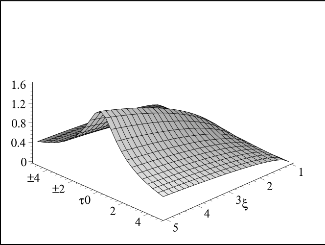
Figure 3: The $(t/\ell,\xi)$ circumference surface, for ${\cal M}=1$, , with $\Lambda<0$.

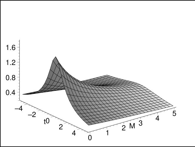
Figure 4: The $(t/\ell,{\cal M})$ circumference surface, for $\xi=3$, , with $\Lambda<0$.

Another useful way of understanding the effect of the point mass on the spacetime is to choose $\tau=\frac{1}{\ell}\tan\left(\frac{t}{\ell}\right)$ as in eq. (37). In these coordinates $t$ is the proper time when $M=0$. This gives

$${\mathfrak{C}}=2\ell\cos\left(\frac{t}{\ell}\right)\text{arctanh}\left(\frac{\xi\sqrt{\frac{\left(\kappa M\ell\right)^{2}}{16}\cos^{2}\left(\frac{t}{\ell}\right)+(\xi^{2}-1)}-\frac{\kappa M\ell}{4}\cos\left(\frac{t}{\ell}\right)}{\frac{\left(\kappa M\ell\right)^{2}}{16}\cos^{2}\left(\frac{t}{\ell}\right)+\xi^{2}}\right)$$ (140)

where now $H=\frac{2{\mathfrak{C}}}{\kappa\ell^{2}}\sec^{2}\left(t/\ell\right)$, and $t\in\left[-\frac{\pi\ell}{2},\frac{\pi\ell}{2}\right]$.  Figures 5 and 6 show the evolution of the circumference over the full range of $t$ for various values of ${\cal M}$ and $\xi$ respectively. As the mass increases, the circumference of the circle more rapidly approaches its decreasing maximal value, hovering there for most of the evolution of the spacetime.

Figure 5: The same plot as in fig 1 but in proper time coordinates $\tau=\frac{1}{\ell}\tan\left(\frac{t}{\ell}\right)$, with $\Lambda<0$.

Figure 6: The same plot as in fig 2 but with $\tau=\frac{1}{\ell}\tan\left(\frac{t}{\ell}\right)$, with $\Lambda<0$.

By replacing $t\rightarrow\ell^{2}/t$ in (139) (so that $\tau=-1/t$) a “big bang” cosmology is obtained, in which the Hamiltonian is divergent at $t=0$ and the spacetime expands from that point. In these coordinates, the evolution of the circumference is illustrated in figure 7

Figure 7: Circumference plotted against time in the “big bang” coordinates, with $\Lambda<0$. Here $\xi=2$ and the values of ${\cal M}$ are respectively $0$ (solid), $1$ (hash), $4$ (dash), $10$ (dot).

with both the negative cosmological constant and the mass contributing to the deceleration. For $M=0$ the circumference asymptotes to a value of unity in units of $2\ell$ due to the decelerating effects of the negative cosmological constant.

The last choice of time coordinate I shall consider is that of the conformally flat coordinates eq. (77), for which $\tau=\sinh\left(t/\ell\right)/\ell$. This gives

$${\mathfrak{C}}=2\ell\text{sech}\left(\frac{t}{\ell}\right)\text{arctanh}\left(\frac{\xi\sqrt{\frac{\left(\kappa M\ell\right)^{2}}{16}\text{sech}^{2}\left(\frac{t}{\ell}\right)+(\xi^{2}-1)}-\frac{\kappa M\ell}{4}\text{sech}\left(\frac{t}{\ell}\right)}{\frac{\left(\kappa M\ell\right)^{2}}{16}\text{sech}^{2}\left(\frac{t}{\ell}\right)+\xi^{2}}\right)$$ (141)

for the circumference and $H=\frac{2{\mathfrak{C}}}{\kappa\ell^{2}}\cosh\left(t/\ell\right)$ for the Hamiltonian. The Hamiltonian is constant for $M=0$,. and so in these coordinates departures from constant energy signal the presence of  a point mass.  Figures  8 and 9 plot the Hamiltonian in units of $\kappa\ell^{2}/2$ for various values of  ${\cal M}$ and $\xi$ respectively.

Figure 8: Hamiltonian plotted against time in conformally flat coordinates for$\ \xi=2$ for differing values of ${\cal M}=0$ (solid), $1$ (hash), $4$ (dash), $10$ (dot), with $\Lambda<0$.

Figure 9: Hamiltonian plotted against time in conformally flat coordinates for ${\cal M}=1$ for differing values of $\xi=2$ (solid), $3$ (hash), $5$ (dash), $10$ (dot), with $\Lambda<0$.

4.2.2 $\Lambda=0$

For $\Lambda=0$ the circumference undergoes a perturally decelerating expansion due to the presence of the point mass. Setting $\tau=t/\ell^{2}$, the Hamiltonian is again $H=\frac{2{\mathfrak{C}}}{\kappa\ell^{2}}$ and

$${\mathfrak{C}}=\frac{2\ell^{2}}{\left|t\right|}\text{arctanh}\left(\frac{\xi\sqrt{\frac{\left(\kappa M\ell\right)^{2}}{16}+(\xi^{2}-1)\left(t/\ell\right)^{2}}-\frac{\kappa M\ell}{4}}{\frac{\left(\kappa M\ell\right)^{2}}{16}+\xi^{2}\left(t/\ell\right)^{2}}\left|t/\ell\right|\right)$$ (142)

where the spatial coordinate $x$ has been rescaled as before and $\ell$ is now an arbitrary constant. In these coordinates the evolution of the spacetime is qualitatively similar to that given in figures 1 – 4: the circumference expands from zero radius at $t=-\infty$ to some maximal value and then reverses its evolution. This maximal value increases as the mass decreases, diverging at $M\rightarrow 0$, in which case the curves bifurcates into two distinct spactime evolutions, one expanding to infinity and one contracting from infinity, that are related to one another under $t\leftrightarrow-t$.

A more useful comparison is made in coordinates where $\tau=-1/t$, for which $t$ is now the proper time when $M=0$. The circumference becomes

$${\mathfrak{C}}=2\left|t\right|\text{arctanh}\left(\frac{\xi\sqrt{\frac{\left(\kappa M\ell\right)^{2}}{16}\left(t/\ell\right)^{2}+(\xi^{2}-1)}-\frac{\kappa M\ell}{4}\left|t/\ell\right|}{\frac{\left(\kappa M\ell\right)^{2}}{16}\left(t/\ell\right)^{2}+\xi^{2}}\right)$$ (143)

and the Hamiltonian $H=\frac{2{\mathfrak{C}}}{\kappa t^{2}}$ , which diverges at $t=0$.  Figures 10 and 11 illustrate how the expansion of the circumference is altered by the point mass in these coordinates. For $M=0$ it expands indefinitely from a “big bang” as a linear function of $t$, whereas for $M\neq 0$  it asymptotes to

$$\lim_{t\rightarrow\infty}{\mathfrak{C}=}\frac{8(\xi-1)}{\kappa M\text{ }}$$ (144)

approaching this value as $1/t^{2}$. The rate of deceleration is decreased for increasing $\xi$.

Figure 10: Circumference plotted against time for $\xi=2$ for differing values of ${\cal M}=0$ (solid), $1/2$ (hash), $2$ (dash), $10$ (dot), with $\Lambda=0$.

Figure 11: Circumference plotted against time for ${\cal M}=1/2$ for differing values of $\xi=2$ (solid), $3$ (hash), $5$ (dash), $10$ (dot), with $\Lambda=0$.

This is similar to the expansion in the big-bang coordinates for the $\Lambda<0$ case, except that for $M=0$ there is no deceleration.

In coordinates which are conformally flat for $M=0$, the circumference is

$${\mathfrak{C}}=2\ell\exp\left(-t/\ell\right)\text{arctanh}\left(\frac{\xi\sqrt{\frac{\left(\kappa M\ell\right)^{2}}{16}+(\xi^{2}-1)e^{2t/\ell}}-\frac{\kappa M\ell}{4}}{\frac{\left(\kappa M\ell\right)^{2}}{16}+\xi^{2}e^{2t/\ell}}e^{t/\ell}\right)$$ (145)

with $H=\frac{2{\mathfrak{C}}}{\kappa t^{2}}\exp\left(t/\ell\right)$, which is constant. Figure 12  plots the time dependence of the Hamiltonian in these coordinates for various values of ${\cal M}$.

Figure 12: Hamiltonian plotted against time in conformally flat coordinates for$\ \xi=2$ for differing values of ${\cal M}=0$ (solid), $1$ (hash), $4$ (dash), $10$ (dot), with $\Lambda=0$.

Except for $M=0$, the Hamiltonian vanishes as $t\rightarrow-\infty$, and changes to a value of $\frac{2\text{arccosh}\xi}{\kappa t}$ around $t=0$, exponentially rapidly approaching this value for large $t.$

4.2.3 $\Lambda>0$

For $\Lambda>0$ a wide variety of possibilities emerge for the evolution of the circumference. This is because the attractive gravitational character of the mass is offset by the ‘repulsive’ gravitational character of the positive cosmological constant.

Consider first the behaviour in the proper-time coordinates (53),  where $\tau=-\coth\left(t/\ell\right)/\ell.$ From (112) this gives for the circumference

$${\mathfrak{C}}=2\ell\sinh\left(\frac{t}{\ell}\right)\text{arctanh}\left(\frac{\xi\sqrt{\frac{\left(\kappa M\ell\right)^{2}}{16}\sinh^{2}\left(\frac{t}{\ell}\right)+(\xi^{2}-1)}-\frac{\kappa M\ell}{4}\sinh\left(\frac{t}{\ell}\right)}{\frac{\left(\kappa M\ell\right)^{2}}{16}\sinh^{2}\left(\frac{t}{\ell}\right)+\xi^{2}}\right)$$ (146)

where $H=\frac{2{\mathfrak{C}}}{\kappa\ell^{2}}$csch${}^{2}\left(t/\ell\right)$. For $M=0$ the spacetime exponentially expands as in the dish scenario as described by (54).  However for $M\neq 0$ the exponential expansion halts for sufficiently large $t$, and the circumference asymptotes exponentially to the fixed value  (144), as shown in fig. 13.

Figure 13: Circumference plotted against the proper time choice for $\xi=2$ for differing values of ${\cal M}=0$ (solid), $0.1$ (hash), $1/2$ (dash), $4$ (dot), with $\Lambda>0$.

For the generalization of the candlestick scenario (48), a wider variety of possibilities ensues.  The proper time coordinate choice is now $\tau=\tanh\left(t/\ell\right)/\ell$, yielding

$${\mathfrak{C}}=2\ell\cosh\left(\frac{t}{\ell}\right)\left[\arctan\left(\frac{\xi\sqrt{\frac{\left(\kappa M\ell\right)^{2}}{16}\cosh^{2}\left(\frac{t}{\ell}\right)+(1-\xi^{2})}-\frac{\kappa M\ell}{4}\cosh\left(\frac{t}{\ell}\right)}{\frac{\left(\kappa M\ell\right)^{2}}{16}\cosh^{2}\left(\frac{t}{\ell}\right)-\xi^{2}}\right)+n\pi\right]$$ (147)

The Hamiltonian $H=\frac{2{\mathfrak{C}}}{\kappa\ell^{2}}$sech${}^{2}\left(t/\ell\right)$ and does not diverge anywhere.   The spacetime  behaves completely differently for $n=0$ than for the candlestick metric (48): the circumference evolves from the asymptotic value $\frac{8(\xi-1)}{\kappa M\text{ }}$ at $t=-\infty$, grows to some maximal size, and then recontracts, reversing its evolution to $t=+\infty$,  When the left-hand inequality of (129) is saturated, a cusp develops at $t=0$, as illustrated in fig. 14.

Figure 14: Circumference plotted against the proper time choice for $\xi=2$ for differing values of ${\cal M}=\sqrt{3}$ (solid), $1.8$ (hash), $2$ (dash), $3$ (dot), with $\Lambda>0$, from eq. (147) .  Note the presence of the cusp for ${\cal M}=\sqrt{3}$.

For $n>0$, the only constraint on $\xi$ is $\sqrt{1+\frac{\left(\kappa M\right)^{2}}{8\Lambda}}>\left|\xi\right|$.  The evolution is now analogous to that of the metric (48), with the circle having a large initial circumference that exponentially shrinks with proper time to a minimal value and then exponentially expands again to infinity, each labelled by a positive integer $n$.  Fig. 15 shows a set of typical values for $n=1$; larger values of $n$ follow a similar pattern, but with the minimal value shifted up by $2\ell\left(n-1\right)\pi$. The effect of the point mass is to reduce the size of the minimal circumference.

Figure 15: Circumference plotted against the proper time choice for $\xi=2$ for differing values of ${\cal M}=2$ (solid), $3$ (hash), $5$ (dash), $10$ (dot), with $\Lambda>0$, from eq. (147), with $n=1$ .

If $\xi<0$, the effect of the point mass is to enlarge the size of the minimal circumference; fig 16 provides an illustration.

Figure 16: The same situation as in fig 15, except that $\xi=-2$.

For most values of $\xi$ there is a unique minimal circumference. However for a certain range

$$\sqrt{1+\frac{\left(\kappa M\ell\right)^{2}}{16}}>\left|\xi\right|>\sqrt{1+\frac{\left(\kappa M\right)^{2}}{8\Lambda}}\left(1-\varepsilon\right)$$ (148)

where

$$\varepsilon=\frac{\left(\frac{\kappa M\ell}{4}\right)^{4}}{\left[\frac{\kappa M\ell}{4}+\left(1+\frac{\left(\kappa M\ell\right)^{2}}{16}\right)\left(\arctan\left(\frac{\kappa M\ell}{4}\right)+n\pi\right)\right]}$$ (149)

there is a local maximum in the evolution of the circumference at $t=0$.  Beginning at $t=-\infty$, the circumference evolves from infinity to a minimal value, expands to a local maximum at $t=0$, and then reverses its evolution.  If the left-hand bound given in (148) is saturated, a cusp develops at $t=0$.  Fig. 17 illustrates the effect near $\xi=2$ (i.e. for $\frac{\kappa M\ell}{4}=\sqrt{3}$) .  For this range of parameters, the candlestick gets a bulge near $t=0$ due to the presence of the point mass.

Figure 17: A close-up near $t=0$ of the evolution of the circumference in (147) for $\Lambda>0$ , $n=1$, and $\frac{\kappa M\ell}{4}=\sqrt{3}$ in proper time coordinates, for $\xi=$ $\sqrt{1+\frac{\left(\kappa M\right)^{2}}{8\Lambda}}$ (solid), $\xi=\sqrt{1+\frac{\left(\kappa M\right)^{2}}{8\Lambda}}\left(1-\varepsilon/4\right)$ (hash), $\xi=\sqrt{1+\frac{\left(\kappa M\right)^{2}}{8\Lambda}}\left(1-\varepsilon\right)$ (dash), $\xi=\sqrt{1+\frac{\left(\kappa M\right)^{2}}{8\Lambda}}\left(1-2\varepsilon\right)$ (dot),

For $\xi<0$ this effect does not occur, except that the first-derivative of the evolution of the circumference becomes discontinuous at $t=0$.

Setting next $\tau=t/\ell^{2}$ and $\left|\Lambda\right|=2/\ell^{2}\,$ yields from (112)

$${\mathfrak{C}}=\frac{2\ell}{\sqrt{\left(t/\ell\right)^{2}-1}}\text{arctanh}\left(\frac{\xi\sqrt{\frac{\left(\kappa M\ell\right)^{2}}{16}+(\xi^{2}-1)(\left(t/\ell\right)^{2}-1)}-\frac{\kappa M\ell}{4}}{\frac{\left(\kappa M\ell\right)^{2}}{16}+\xi^{2}(\left(t/\ell\right)^{2}-1)}\sqrt{\left(t/\ell\right)^{2}-1}\right)$$ (150)

for the proper circumference of the circle. The Hamiltonian is $H=\frac{2{\mathfrak{C}}}{\kappa\ell^{2}}$ and the spatial coordinate $x$ has been rescaled as before. This solution matches analytically onto the $n=0$ solution of (127), which is

$${\mathfrak{C}}=\frac{2\ell}{\sqrt{1-\left(t/\ell\right)^{2}}}\left(\arctan\left(\frac{\xi\sqrt{\frac{\left(\kappa M\ell\right)^{2}}{16}+(1-\xi^{2})(1-\left(t/\ell\right)^{2})}-\frac{\kappa M\ell}{4}}{\frac{\left(\kappa M\ell\right)^{2}}{16}-\xi^{2}(1-\left(t/\ell\right)^{2})}\sqrt{1-\left(t/\ell\right)^{2}}\right)+n\pi\right)$$ (151)

provided $\xi<\sqrt{1+\frac{\left(\kappa M\right)^{2}}{8\Lambda}}$. In this case the behaviour of the circumference is similar (though not identical) to that described in eq. (139): it expands from zero at $t=-\infty$ to a maximum and back to zero again, with a cusp developing if the left-hand bound of (129) is saturated, as shown in fig.  18.

Figure 18: Circumference plotted against time as given in (150,151), with the choice $\xi=2$ for differing values of ${\cal M}=\sqrt{3}$(solid), $2$ (hash), $3$ (dash), $5$ (dot), with $\Lambda>0$.

For $n>0$ the behaviour of the spacetime is analogous to that described by eq. (147) and fig. (17): the circumference shrinks from infinity beginning at $t=\ell$ down to a minimum, expands to a local maximum  at $t=0$ if (148) is satisfied, and then reverses its evolution.

For the“big bang” coordinate choice, again replace $t\rightarrow\ell^{2}/t$  in (150,151) to respectively obtain

$${\mathfrak{C}}=\frac{2\left|t\right|}{\sqrt{1-\left(t/\ell\right)^{2}}}\text{arctanh}\left(\frac{\xi\sqrt{\frac{\left(\kappa M\ell\right)^{2}}{16}\left(t/\ell\right)^{2}+(\xi^{2}-1)(1-\left(t/\ell\right)^{2})}-\frac{\kappa M\ell}{4}\left|t/\ell\right|}{\frac{\left(\kappa M\ell\right)^{2}}{16}\left(t/\ell\right)^{2}+\xi^{2}(1-\left(t/\ell\right)^{2})}\sqrt{1-\left(t/\ell\right)^{2}}\right)$$ (152)

$${\mathfrak{C}}=\frac{2\left|t\right|}{\sqrt{\left(t/\ell\right)^{2}-1}}\left(\arctan\left(\frac{\xi\sqrt{\frac{\left(\kappa M\ell\right)^{2}}{16}\left(t/\ell\right)^{2}+(1-\xi^{2})(\left(t/\ell\right)^{2}-1)}-\frac{\kappa M\ell}{4}\left|t/\ell\right|}{\frac{\left(\kappa M\ell\right)^{2}}{16}\left(t/\ell\right)^{2}-\xi^{2}(\left(t/\ell\right)^{2}-1)}\sqrt{\left(t/\ell\right)^{2}-1}\right)+n\pi\right)$$ (153)

and these solutions analytically continue into each other for $n=0$.  The circumference evolves from zero size and asymptotes to its maximal size given by the limit

$$\lim_{t\rightarrow\infty}{\mathfrak{C}}\left(n=0\right)=2\ell\left(\arctan\left(\frac{\xi\sqrt{\frac{\left(\kappa M\ell\right)^{2}}{16}+(1-\xi^{2})}-\frac{\kappa M\ell}{4}}{\frac{\left(\kappa M\ell\right)^{2}}{16}-\xi^{2}}\right)+n\pi\right)$$ (154)

with $n=0$, and is described by fig. 19

Figure 19: Circumference plotted against “big bang” time as given in (152,153), with the choice $\xi=2$ for differing values of ${\cal M}=\sqrt{3}$(solid), $2$ (hash), $4$ (dash), $10$ (dot), with $\Lambda>0$ and $n=0.$

For $n>1$, the circumference contracts from infinity beginning at $t=1$, and again asymptotes to the value (154), as shown in fig. 20.

Figure 20: Circumference plotted against “big bang” time as given in (152,153), with the choice $\xi=2$ for differing values of ${\cal M}=\sqrt{3}$(solid) and $4$ (dash), with $\Lambda>0$ and $n=1.$

There is also a scenario which is the time-reversed version of this, and is obtained from (153) for negative values of $t$.

Finally, consider the situation using conformal coordinates where $\dot{\tau}=\sqrt{\pm\left(\tau^{2}-\Lambda/2\right)}$.  Eqs. (112,127) respectively become

$${\mathfrak{C}}=\frac{2\ell}{\sinh(t/\ell)}\text{arctanh}\left(\frac{\xi\sqrt{\frac{\kappa^{2}M^{2}}{16}+(\xi^{2}-1)\sinh^{2}(t/\ell)}-\frac{\kappa M}{4}}{\frac{\kappa^{2}M^{2}}{16}+\xi^{2}\sinh^{2}(t/\ell)}\sinh(t/\ell)\right)$$ (155)

$${\mathfrak{C}}=\frac{2\ell}{\left|\sin(t/\ell)\right|}\left[\arctan\left(\frac{\xi\sqrt{\frac{\kappa^{2}M^{2}}{16}+(1-\xi^{2})\sin^{2}(t/\ell)}-\frac{\kappa M}{4}}{\frac{\kappa^{2}M^{2}}{16}-\xi^{2}\sin^{2}(t/\ell)}\left|\sin(t/\ell)\right|\right)+n\pi\right]$$ (156)

with respective Hamiltonians $H=\frac{2{\mathfrak{C}}}{\kappa t^{2}}\sinh(t/\ell)$, $H=\frac{2{\mathfrak{C}}}{\kappa t^{2}}\sin(t/\ell)$.  When the circumference is given by (155), it evolves from zero size to a maximal value at $t=0$, and then reverses its evolution, similar to the situation illustrated in fig.  The corresponding value of the Hamiltonian decreases from unity to zero when the maximal expansion is attained, and then increases back to unity from zero again, as shown in fig. 21.

Figure 21: Hamiltonian associated with eq. (155) plotted against time in conformally flat coordinates for$\ \xi=2$ for differing values of ${\cal M}=0$ (solid), $1$ (hash), $3$ (dash), $10$ (dot), with $\Lambda>0$.

The negative values of the Hamiltonian arise because of the choice of  time coordinate;  $\tau$ is decreasing as the circumference is increasing in the first half of the evolution.

When the circumference is given by (156) the situation is markedly different.  For $n=0$ it undergoes periodic oscillations between $\pm 2\ell\arctan\left(\frac{\xi\sqrt{\frac{\kappa^{2}M^{2}}{16}+(1-\xi^{2})}-\frac{\kappa M}{4}}{\frac{\kappa^{2}M^{2}}{16}-\xi^{2}}\right)$, with cusps developing whenever the left-hand side of eq.(148) is saturated, as shown in fig.22.

Figure 22: Circumference given in (156) plotted against time with the choice $\xi=2$ for differing values of ${\cal M}=\sqrt{3}$(solid, with cusp), $2$ (hash), $4$ (dash), $10$ (dot), with $\Lambda>0$ and $n=0.$ The dashed line for ${\cal M}=4$ looks almost solid because of the close proximity of the dash marks.

The accompanying Hamiltonian oscillates between positive and negative values as shown in fig. 23.

Figure 23: The corresponding Hamiltonian for the cases shown in (22) plotted against time with the choice $\xi=2$ for differing values of ${\cal M}=\sqrt{3}$(solid), $2$ (hash), $4$ (dash), $10$ (dot), with $\Lambda>0$ and $n=0.$

For $n>1$, the circumference diverges at $t=0$, decreases to some minimal value, and then expands out to infinity at $t=\pi\ell$, with the Hamiltonian correspondingly increasing from $4\pi/\kappa\ell$ to a maximum and then decreasing back to this value. If the inequality (148) is respected, then there will be a local maximum at $t=\pi/2$ in the circumference, but not in the Hamiltonian. Figs. 24 and 25 depict the behaviours.

Figure 24: Circumference given in (156) plotted against time with the choice $\xi=2$ for differing values of ${\cal M}=\sqrt{3}$(solid, with cusp), $2$ (hash), $4$ (dash), $10$ (dot), with $\Lambda>0$ and $n=1.$

Figure 25: The corresponding Hamiltonian for the cases shown in (24) plotted against time with the choice $\xi=2$ for differing values of ${\cal M}=\sqrt{3}$(solid), $2$ (hash), $4$ (dash), $10$ (dot), with $\Lambda>0$ and $n=1.$

For $t\in\left[2n\pi\ell,\left(2n+1\right)\pi\ell\right]$ the patterns shown in figs. 24, 25 are the same. However for $t\in\left[\left(2n+1\right)\pi\ell,2n\pi\ell\right]$ the circumference in (156) becomes negative, and the solution is invalid.

5 Summary

The canonical formulation of lineal gravity on a circle yields a rich set of interesting spacetime dynamics when coupled to point particles.  The explicit solutions obtained in this paper for the single-particle case represent a new set of exact solutions to the equations of lineal gravity, and illustrate the broad range of spacetime behaviours that can arise for a self-gravitating system in a compact spacetime.

The formalism developed in this paper could be used to treat a variety of related problems, including solving the 2-body problem (with and without charge), generalization to other dilatonic theories of gravity, exploring new solutions to the static balance problem (extending the work of ref. [17]), and developing a statistical mechanics for self-gravitating systems in compact spacetimes.

A very interesting open problem is the quantization of the system described here.  The lineal gravity system described here has $(N-1)$ degrees of freedom, which is zero for a single point particle.  The nonlinearities of the system here are much less severe than in $(3+1)$ dimensional gravity, and so the prospects for achieving this goal do not seem too remote. Work on this area is in progress.

Acknowledgements

I am grateful to V. Moncreif for interesting discussions concerning this work, and to T. Ohta for helpful correspondence. I am grateful for the hospitality of the Institute for Theoretical Physics at Santa Barbara, where part of this work was carried out. This research was supported by the Natural Sciences and Engineering Research Council of Canada.

References

- [1] H. Koyama and T. Kinoshi, astro-ph/0008208
- [2] See B.N. Miller and P. Youngkins, Phys. Rev. Lett. 81 4794 (1998); K.R. Yawn and B.N. Miller, Phys. Rev. Lett. 79 3561 (1997) and references therein.
- [3] R.B. Mann and P. Chak, gr-qc/0101106
- [4] A. Bellini, M. Ciafaloni and P. Valtancoli, Nucl. Phys. B462 (1996) 453; L. Cantini, P. Menotti, D. Seminara, hep-th/0012022.
- [5] T. Ohta and R.B. Mann, Class. Quant. Grav. 13 (1996) 2585.
- [6] R.B. Mann and T. Ohta, Phys. Rev. D57 (1997) 4723; Class. Quant. Grav. 14 (1997) 1259.
- [7] R.B. Mann, D. Robbins and T. Ohta, Phys. Rev. Lett. 82 (1999) 3738.
- [8] R.B. Mann, D. Robbins and T. Ohta, Phys. Rev. D60 (1999) 104048.
- [9] R.B. Mann, D. Robbins, T. Ohta and M. Trott, Nucl. Phys. B590 367.
- [10] R.B. Mann, G. Potvin and M. Raiteri, Class. Quant. Grav. 17 (2000) 4941.
- [11] V. Moncreif, J. Math. Phys. 30 (1989) 2907.
- [12] R.B. Mann, Found. Phys. Lett. 4 (1991) 425; R.B. Mann, Gen. Rel. Grav. 24 (1992) 433.
- [13] S.F.J. Chan and R.B. Mann, Class. Quant. Grav. 12 (1995) 351.
- [14] R. Jackiw, Nucl. Phys. B 252, 343 (1985); C. Teitelboim, Phys. Lett. B 126, 41, (1983).
- [15] T. Banks and M. O’ Loughlin, Nucl. Phys. B362 (1991) 649; R.B. Mann, Phys. Rev.D47 (1993) 4438.
- [16] R. Arnowitt, S. Deser and C.W. Misner, Phys. Rev 120 (1960) 313.
- [17] R.B. Mann and T. Ohta, Class. Quant. Grav. 17 (2000) 4059.