Metric-based Hamiltonians, null boundaries, and isolated horizons

Abstract

We extend the quasilocal (metric-based) Hamiltonian formulation of general relativity so that it may be used to study regions of spacetime with null boundaries. In particular we use this generalized Brown-York formalism to study the physics of isolated horizons. We show that the first law of isolated horizon mechanics follows directly from the first variation of the Hamiltonian. This variation is not restricted to the phase space of solutions to the equations of motion but is instead through the space of all (off-shell) spacetimes that contain isolated horizons. We find two-surface integrals evaluated on the horizons that are consistent with the Hamiltonian and which define the energy and angular momentum of these objects. These are closely related to the corresponding Komar integrals and for Kerr-Newman spacetime are equal to the corresponding ADM/Bondi quantities. Thus, the energy of an isolated horizon calculated by this method is in agreement with that recently calculated by Ashtekar and collaborators but not the same as the corresponding quasilocal energy defined by Brown and York. Isolated horizon mechanics and Brown-York thermodynamics are compared.

1 Introduction

In the almost 30 years since its initial discovery by Bekenstein [2] and Hawking [3], black hole thermodynamics has been one of the most active areas of gravitational research. There have been several reasons for this interest, but perhaps the chief one is that these laws represent one of the few solid links between the classical world of general relativity and the much-sought-after theory of quantum gravity. Just as quantum mechanics gives rise to the statistical mechanics that in turn explains the thermodynamics of condensed matter, it is believed that the laws of quantum gravity will explain the statistical mechanics and therefore thermodynamics of black holes. The advances made by string theory and canonical quantum gravity towards this goal in the last few years are well known (see [4] for a review and references).

That said, there are several ways in which standard black hole thermodynamics differs from the more familiar thermodynamics of everyday materials. Perhaps the most obvious problem with black holes comes from their very definition. While one can easily localize standard thermodynamic systems such as steam engines in spacetime, this is not the case for a black hole. By the standard definition, a black hole is a region of spacetime from which no null or timelike signal can ever escape. Thus, one must know the entire history of a spacetime before one can say with certainty whether or not a particular region is inside a black hole. Such a definition is too unwieldy to use except in the very special case of stationary spacetimes and so one would like to find a more general class of objects that retain the properities of black holes that are essential for thermodynamics, while at the same time being more convenient to identify and study.

A second problem with black hole thermodynamics arises in the definition of thermodynamic quantities such as energy or angular momentum. While the entropy of a black hole is measured at the event horizon itself, in the usual formulation of black hole thermodynamics energy and angular momentum are defined by ADM measurements taken back at infinity. Further, to define the temperature of a black hole one must make reference to Killing vector fields at infinity. Again this is a situation that is alien to less esoteric thermodynamics. One can define the energy of a standard thermodynamic system such as an ice-cube without first having to retreat to the outer reaches of the universe. A local definition of energy is obviously important too if one doesn’t want to include stray galaxies sitting megaparsecs away from a black hole in its total mass. Thus, to give a good formulation of gravitational thermodynamics, we need quasilocal ways to both identify black holes (or some generalization of them) and to measure all of their thermodynamic properties.

Quite recently Ashtekar, Beetle, and Fairhurst proposed a solution to these problems when they defined isolated horizons [5, 6]. Roughly these are closed, non-expanding, null surfaces which are in equilibrium with their surrounding spacetime (though as long as the rest of the spacetime doesn’t disturb the equilibrium of the horizon it may itself be dynamic). In a series of papers following the initial two, those authors and others have studied the geometric properties of various species of isolated horizons and also shown how they naturally fit into the tetrad and spinor Hamiltonian formulations of general relativity. They have provided quasilocal, horizon-based definitions of the thermodynamic properties of isolated horizons and used the Hamiltonian formalism to derive the zeroth and first laws of thermodynamics (see for example [7] for a review of this work and further references).

Of course, Hamiltonian derived definitions of quasilocal energy and even quasilocal thermodynamics are nothing new and there has been an active literature on these subjects for some years (see for example [8, 9] and the references contained therein). In fact, the quasilocal energy community has generally been more ambitious than the isolated horizon one and sought to define the energy of arbitrary regions of spacetime rather than just black holes. Unfortunately, the various definitions tend to disagree on their localizations and no consensus on what is the “correct” quasilocal energy (or even if such a thing exists) has been reached. Nevertheless, there are well developed quasilocal formalisms out there, and it is of interest to see what they have to say about isolated horizons and how their quasilocal definitions relate to the isolated horizon ones.

One of the most popular definitions of quasilocal energy [8] and formulations of quasilocal thermodynamics [10] was proposed by Brown and York in 1993. Starting with the standard Einstein-Hilbert action (with boundary terms) they calculated the first variation of the action. Setting it equal to zero they obtained the equations of motion (in the usual way) plus a set of boundary conditions. Enforcing these boundary conditions causes the variational boundary term to vanish and so ensure that the variational principle is well-defined. The conditions vary according to the original boundary terms of the action and so there is quite a bit of freedom in the whole procedure. That said, for each choice of the action, one can apply a Legendre transform, obtain a Hamiltonian defined on spatial three-surfaces, and so define the quasilocal energy (QLE) of any finite section of that hypersurface as the numerical value of the Hamiltonian evaluated over the region. The trick comes in picking the correct action and it turns out that even in the most simple cases, there is some ambiguity in the definition of the QLE. This ambiguity is interpreted as the freedom to pick the zero-point of the energy. Similar comments may be made about angular momentum, though there the zero-point ambiguity doesn’t arise.

This formalism has many nice characteristics. For example, it reduces to the ADM [8] and Bondi [11] energies in the appropriate infinite limits, while in the limit of a sufficiently small quasilocal region with volume $V$, it reduces to the matter energy $(V\times T_{{\alpha}{\beta}}u^{\alpha}u^{\beta})$ where $T_{{\alpha}{\beta}}$ and $u^{\alpha}$ are respectively local values of the stress-energy tensor and the timelike normal to the spacelike hypersurface [12]. With the help of Euclidean path integral gravity one can use it to (partially) explain black hole thermodynamics (appendix A or [10] for more details). It has even been used to study gravitational tidal heating [13]. However, the formalism as it stands is not quite suitable for studying isolated horizons. Specifically, quasilocal quantities such as energy and angular momentum are defined by sets of observers who evolve in a timelike way. For an isolated horizon, we want to make measurements on the null surface itself which means that such observers must have null (or even spacelike) velocities.

In this paper, we extend the metric-based Hamiltonian perspective to include null boundary surfaces (and classes of observers moving with null or spacelike velocities on those surfaces). The extension is fairly straightforward from a geometrical point of view, but nevertheless the final results differ quite dramatically from those for timelike boundaries. In the standard Brown-York work quasilocal energy (sometimes referred to as the canonical quasilocal energy or CQLE) is essentially measured by the extrinsic curvature of two-surfaces surrounding the system. By contrast, in the new null formulation the QLE of an isolated horizon (which we’ll denote the null QLE or NQLE) is measured not by the expansion of the congruence of null curves that make up the surface (which would be the naive analogue of the extrinsic curvature) but rather by the acceleration of those same curves. Further, while the CQLE suffers from the ambiguity in the aforementioned zero-point terms, for the NQLE this freedom of choice is largely removed by Hamiltonian formalism. This is in agreement with the isolated horizon literature (see for example [6]). Finally, the NQLE measured on an isolated horizon is NOT equal to the CQLE measured on a timelike surface positioned “close” to the horizon. Specifically, in the case of Schwarzschild, the NQLE is $m$ (in agreement with [5]) while the CQLE is $2m$. In fact, for any stationary, axisymmetric isolated horizon in asymptotically flat space, the NQLE is equal to the ADM/Bondi mass of the entire spacetime.

In other ways, however, the results correspond much more closely to those of Brown and York. In particular, the expression for angular momentum on a timelike surface is very closely related to the corresponding expression on a null surface (which in turn we show to be eqivalent to the corresponding Komar formula). Further, basically the same Hamiltonian boundary terms arise on an isolated horizon as those that show up on a timelike surface, though as noted above the roles that they play can be quite different. Also, drawing on the extant work on metric-based Hamiltonians, we can, without much difficulty, carry through the variational calculations explicitly for the phase space of all spacetime configurations rather than just the subspace of solutions to the equations of motion.

This paper is organized in the following manner. Section 2 establishes notation and sign conventions, reviews the definitions and some properties of isolated horizons and considers the constants that characterize these objects. The notation will be an amalgam of that used in the Brown-York tradition of papers with that used in studies of isolated horizons with some new symbols introduced where the systems overlap and clash. Section 3 extends the the work on metric-based Hamiltonians to include systems with null boundaries in general and rigidly rotating horizons (a close cousin of isolated horizons) in particular. We find constraints on possible boundary terms for the Hamiltonian. Section 4, derives the first law of isolated horizon mechanics, proposes an integral boundary term for the Hamiltonian that both satisfies the constraints and is equivalent to the function found in [14], and considers the connection between the quasilocal energy/angular momentum and the corresponding Komar definitions. Section 5 compares the results found for isolated horizons in this paper with the Brown-York quasilocal energy and thermodynamics. Section 6 summarizes the results and appendix A reviews Brown-York thermodynamics.

2 Set-up

The calculations in this paper will be done from a Hamiltonian perspective. As such it will usually be most appropriate to think not of spacetime, but instead of time-dependent tensor fields living and evolving on a spatial three-manifold. At the same time however, many of the quantities appearing in the calculations can most easily be understood as four-dimensional quantitities associated with three-surfaces embedded in a full spacetime. As such, and even though it will create a certain amount of clutter, we will begin by setting things up from a three-dimensional perspective and then “stack” the “instants” of time evolution into a full four-dimensional spacetime. Only then will we define the various sub-species of isolated horizons and then proceed on to the variational calculations. Note that throughout this paper, we’ll use units where $G$ and $c$ are dimensionless and equal to unity.

2.1 The 3D perspective

We begin with the three-dimensional-space plus time perspective, viewing fields as defined in a three-dimensional manifold $\Sigma$ and dynamic with respect to a time coordinate $t$. To emphasize their three-dimensional nature we label them with Latin indices. Figure 1 illustrates this section.

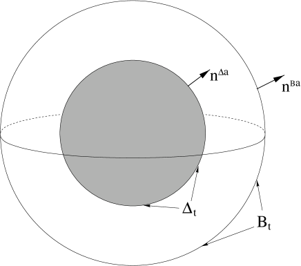
Figure 1: The region $\Sigma_{t}$ with its boundaries and normals.

Let $\Sigma$ be a three-dimensional manifold with Euclidean metric $h_{ab}$, and $\Sigma_{t}\subset\Sigma$ be such that $\Sigma_{t}$ is topologically $S^{2}\times[0,1]$ (where $S^{2}$ is the two-sphere and $[0,1]$ is a real line segment). Label the two-dimensional boundaries of this space $\Delta_{t}$ and $B_{t}$ and refer to them as the “inner” and “outer” boundaries. The induced metrics on these boundaries will be $\sigma^{\Delta}_{ab}$ and $\sigma^{B}_{ab}$ respectively. Next, if $D_{a}$ is the metric compatible covariant derivative on $\Sigma$ then the corresponding induced metrics on the boundaries will be $d_{a}^{\Delta}$ and $d_{a}^{B}$ respectively. Often where there is no chance of confusion we will drop the superscripts on these quantities.

Next, define $n^{\Delta}_{a}$ and $n^{B}_{a}$ as the unit normals to the two-surfaces. They are oriented so that $n^{\Delta}_{a}$ points back “into” and $n^{B}_{a}$ points “out of” $\Sigma_{t}$. Then, one can define the extrinsic curvatures $k^{\Delta}_{ab}=-\frac{1}{2}\mathcal{L}_{n}\sigma^{\Delta}_{ab}=-\sigma^{\Delta c}_{a}\sigma^{\Delta d}_{b}D_{c}n^{\Delta}_{d}$ and $k^{B}_{ab}=-\frac{1}{2}\mathcal{L}_{n}\sigma^{B}_{ab}=-\sigma^{Bc}_{a}\sigma^{Bd}_{b}D_{c}n^{B}_{d}$, where $\mathcal{L}_{v}$ is used to designate a Lie derivative in the direction $v$. The reader should take note of the sign convention used for extrinsic curvatures.

The lapse function $N$ and shift vector $V^{a}$ will define the flow of time relative to this surface in the usual way. That is, $Ndt$ units of proper time pass for every $dt$ units of coordinate time, and an observer swept along by the flow of time will move with velocity $\sqrt{V_{a}V^{a}}/N$ . In particular we will think of the boundaries $\Delta_{t}$ and $B_{t}$ as being made up of such observers, and so their evolution will be guided by the shift vector field. Thus, given the position of $\Delta_{t}$ and $B_{t}$ at any instant $t$, the flow of time determines their position in $\Sigma$ at all future times and therefore the future extent of $\Sigma_{t}$ as well.

In addition to the metric field $h_{ab}$, the Hamiltonian three-surface formulation of general relativity requires a surface-momentum tensor density $P^{ab}$ which is canonically conjugate to the metric (and determines the time rate of charge of the metric). Further, for Einstein-Maxwell spacetimes, there will also be the vector potential one-form $A_{a}$, its canonical conjugate the electric field vector density ${\mathcal{E}}^{a}$ (which apart from its obvious interpretation measures the time rate of change of $A_{a}$), and the Coulomb potential $\Phi$ (which joins the lapse and shift as a Lagrange multiplier).

We now embed all of this in a four-dimensional spacetime.

2.2 The 4D perspective

Let ${\mathcal{M}}$ be a four-dimensional manifold and $M\subset{\mathcal{M}}$ such that $M$ is topologically $[0,1]\times[0,1]\times S^{2}$. Thus, $M$ is “cylindrical” and bounded by four three-dimensional surfaces $\Sigma_{1}$, $\Sigma_{2}$, $\Delta$, $B$ (see figure 2). Next, let $g_{{\alpha}{\beta}}$ be the metric field on ${\mathcal{M}}$ such that $\Sigma_{1}$ and $\Sigma_{2}$ are spacelike, $\Delta$ is null, and $B$ is timelike. Note that we use Greek indices for these four-dimensional quantities. Other situations will be considered later on in the text, but this set-up will allow us to capture all of the essential details for now and for later.

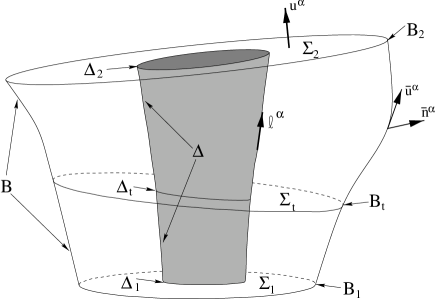
Figure 2: A three-dimensional schematic of $M$ along with its boundaries, normals, and a typical foliation surface. No attempt has been made to have the slope of the boundaries correspond to their “speed”.

Assume that $M$ is foliated by a set of spacelike surfaces $\{\Sigma_{t}:t_{1}\leq t\leq t_{2}\}$ such that $\Sigma_{t_{1}}=\Sigma_{1}$ and $\Sigma_{t_{2}}=\Sigma_{2}$ are the terminal elements of the foliation. These surfaces can then be thought of as “instants” in time and in the usual way, we’ll say that $\Sigma_{t_{\alpha}}$ “happens” before $\Sigma_{t_{\beta}}$ if $t_{\alpha}<t_{\beta}$. A further orientation is implied by choosing to refer to $\Delta$ as the inner boundary and $B$ as the outer boundary. The $\Sigma_{t}$ then induce corresponding foliations $\{\Delta_{t}:t_{1}\leq t_{2}\}$ and $\{B_{t}:t_{1}\leq t\leq t_{2}\}$ on $\Delta$ and $B$ respectively. In the usual ADM/Brown-York formulation of general relativity, these foliations would be independent of the spacetime configuration. However, that will not be the case here and in section 3 we will see how the Hamiltonian formalism restricts the allowed foliations of $\Delta$ (and therefore $M$) if $\Delta$ is an isolated horizon.

Using the spacetime metric $g_{{\alpha}{\beta}}$ one may define normal vectors, projection operators, and metric tensors for the hypersurfaces. Specifically, if $u^{\alpha}$ is the forward pointing unit timelike normal to the $\Sigma_{t}$ then $h_{\alpha}^{\beta}=g_{\alpha}^{\beta}+u^{{\alpha}}u_{\beta}$ is the projection operator into the surface, while $h_{{\alpha}{\beta}}=g_{{\alpha}{\beta}}+u_{\alpha}u_{\beta}$ is the induced spacelike metric. Similarly, if ${\bar{n}}^{\alpha}$ is the outward pointing unit normal to $B$ then $\gamma_{\alpha}^{\beta}=g_{\alpha}^{\beta}-{\bar{n}}_{\alpha}{\bar{n}}^{\beta}$ is the projection operator, and $\gamma_{{\alpha}{\beta}}=g_{{\alpha}{\beta}}-{\bar{n}}_{\alpha}{\bar{n}}_{\beta}$ is the induced timelike metric. For the two-surfaces $B_{t}$, the projection operator maybe written as either of $\sigma_{\alpha}^{\beta}=h_{\alpha}^{\beta}-n_{\alpha}n^{\beta}=\gamma^{\alpha}_{\beta}+{\bar{u}}^{\alpha}{\bar{u}}_{\beta}$ where $n_{\alpha}$ is the outward pointing spacelike unit normal to $B_{t}$ in $\Sigma_{t}$ and ${\bar{u}}_{\alpha}$ is the future pointing timelike unit normal to $B_{t}$ in $B$. The induced metric is then $\sigma_{{\alpha}{\beta}}=h_{{\alpha}{\beta}}-n_{\alpha}n_{\beta}=\gamma_{{\alpha}{\beta}}+{\bar{u}}_{\alpha}{\bar{u}}_{\beta}$. Note that ${\bar{n}}_{\alpha}\neq n_{\alpha}$ and ${\bar{u}}_{\alpha}\neq u_{\alpha}$ unless the foliation surfaces are perpendicular to $B$. That is $\eta\equiv{\bar{u}}^{\alpha}n_{\alpha}=0$.

Next, let $\ell_{\alpha}$ be a null normal to $\Delta$. Thus if $\Delta$ is defined as a level surface of some function $H$ of the spacetime coordinates, $\ell_{\alpha}$ is proportional to $\partial_{\alpha}H$. Further, assume that it points foward in time and into $M$ so that $\ell^{\alpha}u_{\alpha}<0$ and $\ell^{\alpha}n_{\alpha}>0$. However, because $\ell_{\alpha}$ is null, it has no natural normalization. To define the projection operator into $\Delta$, one must invoke an auxilarly null normal $\tilde{\ell}^{\alpha}$ which is also assumed to be perpendicular to $\Delta_{t}$ and which is normalized relative to $\ell_{\alpha}$ so that $\tilde{\ell}^{\alpha}\ell_{\alpha}=-1$. Then if $n_{\alpha}$ is the inward-pointing spacelike unit normal to $\Delta_{t}$, one can write

$$\ell_{\alpha}=\xi(u_{\alpha}+n_{\alpha})\hskip 28.45274pt\mbox{and}\hskip 28.45274pt\tilde{\ell}_{\alpha}=\frac{1}{2\xi}(u^{\alpha}-n^{\alpha})$$ (1)

for some function $\xi$. That said, the projection operator into $\Delta$ is $q_{\alpha}^{\beta}=g_{\alpha}^{\beta}+\tilde{\ell}_{\alpha}\ell^{\beta}$ and the induced metric is $q_{{\alpha}{\beta}}=g_{{\alpha}{\beta}}+\ell_{\alpha}\tilde{\ell}_{\beta}+\tilde{\ell}_{\alpha}\tilde{\ell}_{\beta}$. This metric is, of course degenerate and therefore $q_{{\alpha}{\beta}}$ does not uniquely define its inverse $q^{{\alpha}{\beta}}$ (though this non-uniqueness doesn’t manifest itself in any of the quantities that we use in this paper). It should also be kept in mind that $\ell^{\alpha}$ and $\tilde{\ell}_{\alpha}$ lie in the tangent and cotangent bundles to $\Delta$ respectively while their compatriots $\tilde{\ell}^{\alpha}$ and $\ell_{\alpha}$ do not. The projection operator into $\Delta_{t}$ is $\sigma_{\alpha}^{\beta}=g_{\alpha}^{\beta}+\ell_{\alpha}\tilde{\ell}^{\beta}+\tilde{\ell}_{\alpha}\ell^{\beta}=g_{\alpha}^{\beta}+u_{\alpha}u^{\beta}-n_{\alpha}n^{\beta}$. The induced metric is then $\sigma_{{\alpha}{\beta}}=g_{{\alpha}{\beta}}+\ell_{\alpha}\tilde{\ell}_{\beta}+\tilde{\ell}_{\alpha}\ell_{\beta}=g_{{\alpha}{\beta}}+u_{\alpha}u_{\beta}-n_{\alpha}n_{\beta}$. Note that $\sigma_{{\alpha}{\beta}}=q_{{\alpha}{\beta}}$.

The metric compatible covariant derivative on ${\mathcal{M}}$ will be $\nabla_{\alpha}$ which in turn will induce $D_{\alpha}$ as the metric compatible derivative on $\Sigma_{t}$, $d^{\Delta}_{\alpha}$ on $\Delta_{t}$, and $d^{B}_{\alpha}$ on $B_{t}$. $\triangle_{\alpha}$ will be the induced covariant derivative on $\Delta$. Note that it is compatible with $q_{{\alpha}{\beta}}$, though not uniquely determined by it since that metric is degenerate.

The extrinsic curvatures of these hypersurfaces may be defined as follows. $K_{{\alpha}{\beta}}=-\frac{1}{2}\mathcal{L}_{u}h_{{\alpha}{\beta}}=-h_{\alpha}^{\gamma}\nabla_{\beta}u_{\gamma}$ is the extrinsic curvature of $\Sigma_{t}$ in $M$, $k_{{\alpha}{\beta}}=-\sigma_{\alpha}^{\gamma}\sigma_{\beta}^{\delta}\nabla_{\gamma}n_{\delta}$, is the extrinsic curvature of $B_{t}$ in $\Sigma_{t}$, and $l_{{\alpha}{\beta}}=-\sigma_{\alpha}^{\gamma}\sigma_{\beta}^{\delta}\nabla_{\gamma}u_{\delta}$ is the extrinsic curvature of $B_{t}$ with respect to the normal $u_{\alpha}$. Each of these last two quantities may be considered to be defined for $\Delta_{t}$ or $B_{t}$ as appropriate. Contracted with the appropriate metric tensors these become $K$, $k$, and $l$. The addition of a bar over any of these indicates that they are to be calculated with respected to the “barred” rather than “unbarred” normal. For example $\bar{l}=-\sigma^{{\alpha}{\beta}}\nabla_{\alpha}{\bar{u}}_{\beta}$.

On $\Delta$, the analogous quantity is $\theta_{{\alpha}{\beta}}=q_{\alpha}^{\gamma}q_{\beta}^{\delta}\nabla_{\gamma}\ell_{\delta}=\sigma_{\alpha}^{\gamma}\sigma_{\beta}^{\delta}\nabla_{\gamma}\ell_{\delta}$, which describes the instaneous evolution of the congruences of null geodesics that make up $\Delta$. The reader should take note of the sign convention which is different from that used in the extrinsic curvatures. Then, keeping in mind that $\ell_{\alpha}$ is normal to $\Delta$ so that $\theta_{[\alpha\beta]}=0$, this may be decomposed as

$$\theta_{{\alpha}{\beta}}=\frac{1}{2}\theta\sigma_{{\alpha}{\beta}}+\zeta_{{\alpha}{\beta}}$$ (2)

where $\theta\equiv\sigma^{{\alpha}{\beta}}\theta_{{\alpha}{\beta}}=\frac{1}{{\sqrt{\sigma}}}\mathcal{L}_{\ell}{\sqrt{\sigma}}$ is the null expansion and $\zeta_{{\alpha}{\beta}}\equiv\theta_{{\alpha}{\beta}}-\frac{1}{2}\theta\sigma_{{\alpha}{\beta}}$ is the shear. If $\theta_{{\alpha}{\beta}}=0$, then $q_{{\alpha}{\beta}}$ has a unique compatible covariant derivative $\triangle_{\alpha}$ on $\Delta$.

The flow of time in this manifold is defined by the vector field $T^{\alpha}$ which is chosen to be compatible with the foliation $\{\Sigma_{t}\}$ so that $T^{\alpha}\partial_{\alpha}t=1$. On the hypersurfaces it may be written as $T^{\alpha}=Nu^{\alpha}+V^{\alpha}$ where again $N$ and $V^{\alpha}$ are the lapse and the shift. It is not restricted to being timelike. In fact, near or on $\Delta$ we will expect it to go null or even spacelike. Because of the restriction made in the previous section that the evolution of the boundaries by guided by the time evolution, we know that $T^{\alpha}$ may be written as an element of the tangent bundles $T\Delta$ and $TB$ at the inner and outer boundaries respectively. Specifically, on $\Delta$ we have $T^{\alpha}=\tilde{N}\ell^{\alpha}+\hat{V}^{\alpha}$ where $\tilde{N}\equiv N/\xi$ and $\hat{V}^{\alpha}\equiv\sigma^{\alpha}_{\beta}V^{\beta}$, while on $B$, $T^{\alpha}=\bar{N}{\bar{u}}^{\alpha}+\hat{V}^{\alpha}$ where $\bar{N}\equiv N\lambda$, $\lambda\equiv\sqrt{1+\eta^{2}}$, and (again) $\hat{V}^{\alpha}\equiv\sigma^{\alpha}_{\beta}V^{\beta}$. In section 3 we will see that the allowed forms of $T^{\alpha}$ are restricted at isolated horizons. Again this contrasts with the usual ADM/Brown-York Hamiltonian formulations where $T^{\alpha}$ is an independent background structure.

From this perspective the “instants” are a series of hypersurfaces, rather than a single three-manifold on which dynamic fields evolve. It will be useful to note that the hypersurface momentum $P^{ab}$ which was an independent variable in the previous section, is closely related to the extrinsic curvature $K_{{\alpha}{\beta}}$ and can be written as

$$P^{{\alpha}{\beta}}=\frac{\sqrt{h}}{16\pi}(Kh^{{\alpha}{\beta}}-K^{{\alpha}{\beta}}).$$ (3)

The electromagnetic field in ${\mathcal{M}}$ is described by the vector potential ${\mathcal{A}}_{\alpha}$ which defines the electromagnetic field tensor ${\mathcal{F}}_{{\alpha}{\beta}}=\partial_{\alpha}{\mathcal{A}}_{\beta}-\partial_{\beta}{\mathcal{A}}_{\alpha}$. Then, the three-dimensional vector potential is $A_{\alpha}=h_{\alpha}^{\beta}{\mathcal{A}}_{\beta}$, the Coulomb potential is $\Phi=-{\mathcal{A}}_{\alpha}u^{\alpha}$, and the electric field density is ${\mathcal{E}}^{\alpha}\equiv-\sqrt{h}/(4\pi){\mathcal{F}}^{{\alpha}{\beta}}u_{\beta}$. Throughout this paper we will assume that a single ${\mathcal{A}}_{\alpha}$ can be used to cover the entire region ${\mathcal{M}}$. This assumption means that the electromagnetic $U(1)$ gauge bundle will be trivial and therefore there are no magnetic charges in ${\mathcal{M}}$ – including magnetically charged black holes. Results for magnetically charged spacetimes can be found using electromagnetic duality.

It should also be kept in mind that constant $t$ surfaces in Scwharzschild/Kerr spacetime in the usual static/stationary coordinates are NOT examples of the $\Sigma_{t}$ surfaces that we are considering here. As is well known, such constant $t$ surfaces go null at the event horizon and timelike inside of it. Our $\Sigma_{t}$ are restricted to remain spacelike and so one should instead think of a foliation such as that induced by Painleve-Gullstand-type coordinates. These are analogous to Eddington-Finkelstein coordinates except that they are tied to infalling timelike rather than spacelike geodesics. Descriptions of these in spherically symmetric and Kerr spacetimes may be found in [20] and [21] respectively.

2.3 Review of isolated horizons

This section reviews the definitions of the isolated horizon sub-species as well as some of their properties. It is largely based on the relevant sections of [23] and [14] and the reader is directed there for further discussion and derivation of the definitions and results.

2.3.1 Definitions

Definition 1

A null surface $\Delta$ is a non-expanding horizon if: i) its null expansion $\theta$ is zero everywhere on $\Delta$ for any null normal $\ell^{\alpha}$ ii) all the equations of motion hold at $\Delta$, and iii) the stress tensor $T_{{\alpha}{\beta}}$ of matter fields is such that $-T_{\alpha}^{\beta}\ell^{\alpha}$ is future directed and causal for any null normal $\ell^{\alpha}$.

A couple of notes are in order on these conditions. First, it is trivial to check that if conditions i) and iii) hold for any null normal vector field $\ell^{\alpha}$ then they will hold for all such vector fields and so the definition isn’t based on the normalization of $\ell^{\alpha}$. Second, condition iii) is implied by the dominant energy condition which in particular holds for the Maxwell fields that we consider in this paper. Thus, from our point of view, the only real restriction in the above is that $\theta=0$. Note that any Killing horizon is automatically a non-expanding horizon.

From this simple assumption, many properities follow. First $\Delta$ may be thought of as a congruence of null geodesics. By definition they are surface forming and so their twist $\theta_{[{\alpha}{\beta}]}$ is zero. With the help of the Raychaudri equation one can quickly see that $\theta=0$ then implies that their shear $\zeta_{{\alpha}{\beta}}$ must be zero too. Therefore $\theta_{{\alpha}{\beta}}=0$. It then follows that the induced $\triangle_{\alpha}$ is the unique compatible covariant derivative for $q_{{\alpha}{\beta}}$. From the same calculation the twice contracted stress-energy tensor $T^{{\alpha}{\beta}}\ell_{\alpha}\ell_{\beta}$ = 0 as well. In turn, $T^{{\alpha}{\beta}}\ell_{\alpha}\ell_{\beta}=0$ implies that $f_{\alpha}\equiv\sigma_{\alpha}^{\gamma}F_{{\gamma}{\delta}}\ell^{\delta}$ and $\tilde{f}_{\alpha}\equiv\sigma_{\alpha}^{\gamma}F_{{\gamma}{\delta}}\tilde{\ell}^{\delta}$ are both zero (or equivalently the electric and magnetic fields projected into $\Delta_{t}$ are zero). Physically this means that there is no flux of electromagnetic radiation across the horizon (the relevant component of the Poynting vector is zero).

Moving on, direct calculation and $\theta_{{\alpha}{\beta}}=0$ implies that there exists a one form $\omega_{\alpha}$ such that $q_{\alpha}^{\gamma}\nabla_{\gamma}\ell^{\beta}=\omega_{\alpha}\ell^{\beta}$. Explicitly,

$$\omega_{\alpha}=-\kappa_{\ell}\tilde{\ell}_{\alpha}+\sigma_{\alpha}^{\beta}\ell^{\gamma}\triangle_{\beta}\tilde{\ell}_{\gamma}$$ (4)

where $\kappa_{\ell}\equiv-\tilde{\ell}_{\alpha}\ell^{\beta}\triangle_{\beta}\ell^{\alpha}$ is the acceleration of the null normal $\ell^{\alpha}$. Note that $\omega_{\alpha}$ is defined entirely with respect to quantities intrinsic to $\Delta$. These quantities are, however, dependent on the normalization of $\ell^{\alpha}$ and under a redefinition of the null normal $\ell^{\alpha}\rightarrow\ell^{\prime{\alpha}}=f\ell^{\alpha}$, $\kappa_{\ell^{\prime}}=f\kappa_{\ell}+\mathcal{L}_{\ell}f$ and $\omega^{\prime}_{\alpha}=\omega_{\alpha}+q_{\alpha}^{\beta}\nabla_{\beta}f$.

Definition 2

A non-expanding horizon $\Delta$ becomes a weakly isolated horizon $(\Delta,[\ell])$ if it is equipped with an equivalence class of normals $[\ell]$ such that $q_{\alpha}^{\beta}\mathcal{L}_{\ell}\omega_{\beta}=0$ for all $\ell\in[\ell]$ (where $\ell^{\prime}\sim\ell$ if $\ell^{\prime}=c\ell$ for some constant $c$) and a gauge choice such that $q_{\alpha}^{\beta}\mathcal{L}_{\ell}{\mathcal{A}}_{\beta}=0$.

It quite easy to show that for any non-expanding horizon $\Delta$ there are many choices of $[\ell]$ and gauge choices for the $U(1)$ gauge so that these requirements are satisfied. Further, given such choices, $\kappa_{\ell}$ and $\Phi_{\ell}\equiv-\ell^{\alpha}{\mathcal{A}}_{\alpha}$ are constants over $\Delta$. However, even with the equivalence class chosen it is easy to see from the transformation law given above that the value of $\kappa_{\ell}$ isn’t fixed. A specific $\ell^{\alpha}\in[\ell]$ must be chosen to fix that constant over $\Delta$. Similarly, enough gauge freedom remains so that $\Phi_{\ell}$ may be assigned any value that is desired (though once chosen that value is fixed everywhere on $\Delta$).

Definition 3

A rigidly rotating horizon (RRH) $(\Delta,[\ell],\varphi)$, is a weakly isolated horizon with rotational symmetry. That is, $\mathcal{L}_{\varphi}\ell^{\alpha}=0$, $\mathcal{L}_{\varphi}q_{{\alpha}{\beta}}=0$, $\mathcal{L}_{\varphi}\omega_{\alpha}=0$, $\mathcal{L}_{\varphi}(q_{\alpha}^{\beta}{\mathcal{A}}_{\beta})=0$, and $\mathcal{L}_{\varphi}(q_{\alpha}^{\gamma}q_{\beta}^{\delta}F_{{\gamma}{\delta}})=0$. Further $\varphi^{\alpha}$ has closed, circular orbits, and is normalized so that those orbits have affine length $2\pi$.

We will say that a specific foliation $\Delta_{t}$ is adapted to an RRH if $\varphi^{\alpha}\in T\Delta_{t}$ for all $t$ surfaces. Correspondingly, the time flow field is adapted if $T^{\alpha}=\ell^{\prime{\alpha}}-\Omega_{\varphi}\varphi^{\alpha}$ for some $\ell^{\prime{\alpha}}\in[\ell^{\alpha}]$ and some real constant $\Omega_{\varphi}$. Then, an adapted flow of time selects a specific “normalization” of $\ell^{\alpha}$ and therefore an acceleration $\kappa_{\ell}$ as well. Equivalently, we can say that a choice of $\kappa_{\ell}$ and $\Omega_{\varphi}$ selects a $T^{\alpha}$ on $\Delta$. In that case $T^{\alpha}$ is no longer an independent vector field but is instead defined with respect to quantities intrinsic to the surface.

The canonical example of a rigidly rotating horizon is, of course, the event horizon found in Kerr-Newman spacetime. Any linear combination of the timelike and angular Killing vector fields of the spacetime is then an adapted flow of time. Keep in mind however, that the $t=\mbox{constant}$ surfaces in the standard Boyer-Lindquist coordinates are not spacelike everywhere and therefore not a suitable foliation from the current perspective. Instead one should think in terms of the Painlevé-Gullstand-type coordinates defined in [21].

Finally, for completeness we note that an isolated horizon is a weakly isolated horizon on which $\mathcal{L}_{\ell}$ and $\triangle_{\alpha}$ commute. We won’t actually make use of these in this paper, though often will follow convention and use “isolated horizon” as a generic term for any of the surfaces discussed above.

2.3.2 Constant quantities on the horizons

Given a non-expanding horizon $\Delta$ which is foliated by $\{\Delta_{t}:t_{1}\leq t\leq t_{2}\}$ one can define an area as well as the electric and magnetic charges of each surface $\Delta_{t}$:

$$A_{\Delta}(t) \equiv \int_{\Delta_{t}}d^{2}x{\sqrt{\sigma}},$$ (5)

$$Q_{\Delta}(t) \equiv \int_{\Delta_{t}}d^{2}x{\sqrt{\sigma}}E_{\vdash},\mbox{ and}$$ (6)

$$P_{\Delta}(t) \equiv \int_{\Delta_{t}}d^{2}x{\sqrt{\sigma}}B_{\vdash}.$$ (7)

In the above, $E_{\vdash}\equiv(1/4\pi)F_{{\alpha}{\beta}}\ell^{\alpha}\tilde{\ell}^{\beta}=(1/4\pi)F_{{\alpha}{\beta}}u^{\alpha}n^{\alpha}$ is the normal component of the electric field to $\Delta_{t}$, while $B_{\vdash}\equiv-(1/4\pi)F^{\star}_{{\alpha}{\beta}}\ell^{\alpha}\tilde{\ell}^{\beta}=-(1/4\pi)F^{\star}_{{\alpha}{\beta}}u^{\alpha}n^{\alpha}$ is the normal component of the magnetic field. $F^{\star}_{{\alpha}{\beta}}$ is the dual electromagnetic field tensor. Note too that though we have chosen to write $Q_{\Delta_{t}}$ and $P_{\Delta_{t}}$ in terms of the normals and field tensors, they could also have been written purely as integrals of the pull-backs of the field tensors into $\Delta_{t}$ in which case their independence of the normals is manifest.

Now, it is quite easy to show that if the $\Delta_{t}$ are all closed surfaces (which they are by construction), then these quantities are constant in coordinate time and therefore not dependent on which surface $\Delta_{t}$ they are evaluated on. Therefore, the area and electric and magnetic charges of a non-expanding horizon are invariants of $\Delta$ and independent of the choice of foliation (though of course we have already set $P_{\Delta}=0$ with our assumption that a single ${\mathcal{A}}_{\alpha}$ covers ${\mathcal{M}}$).

Next, moving up a step to weakly isolated horizons and continuing to assume that the $\Delta_{t}$ are closed, one can show that for any constants $c_{1}$ and $c_{2}$ and vector field $v^{\alpha}\in T\Delta$ such that $\pounds_{\ell}v^{\alpha}=0$,

$$C_{\Delta}(v) \equiv \int_{\Delta_{t}}d^{2}x{\sqrt{\sigma}}v^{\alpha}(c_{1}\omega_{\alpha}+c_{2}E_{\vdash}{\mathcal{A}}_{\alpha}),$$ (8)

is a constant in coordinate time, and therefore an invariant of the horizon. In particular, for a rigidly rotating horizon we can define the invariant

$$J_{\Delta}\equiv-\int_{\Delta_{t}}d^{2}x{\sqrt{\sigma}}\varphi^{\alpha}(\omega_{\alpha}/(8\pi)-E_{\vdash}{\mathcal{A}}_{\alpha}),$$ (9)

which in section 4 will be seen to be the angular momentum of the horizon.

Thus for a rigidly rotating horizon we have four geometrically defined invariants: $A_{\Delta}$, $J_{\Delta}$, $Q_{\Delta}$, $P_{\Delta}$ (though we have a priori assumed that the magnetic charge is zero). $\kappa_{\ell}$ and $\Omega_{\varphi}$ are also constants over the surface if we single out a specific adapted flow of time. Later we will see that in order for the Hamiltonian formalism to be well defined, these constants (along with $\Phi_{\ell}$) will have to be functions of $A_{\Delta}$, $J_{\Delta}$, and $Q_{\Delta}$ (though there will be quite a bit of freedom in defining the functions). Therefore, $T^{\alpha}$ will be a “live” vector field and dependent on the spacetime over which it is defined [14].

Finally, for a given adapted time flow,

$$E_{\Delta}(T) \equiv \int_{\Delta_{t}}d^{2}x{\sqrt{\sigma}}T^{\alpha}\left(\omega_{\alpha}/(4\pi)-E_{\vdash}(2{\mathcal{A}}_{\alpha}-\Phi_{\ell}\tilde{\ell}_{\alpha})\right)$$

$$= \frac{\kappa_{\ell}}{4\pi}A_{\Delta}+2\Omega_{\varphi}J_{\Delta}+\Phi_{\ell}Q_{\Delta}$$

is also an invariant. If $E_{\Delta}(T)$ could be interpreted as the energy of an RRH then this would be a Smarr relation for RRHs connecting their energy, angular momentum, and electric charge. In fact, in section 4 we will see that $E_{\Delta}(T)$ is very closely related to the Komar/Bondi energy for a stationary spacetime and so can be taken as the the total energy of the RRH.

With this review under our belts and promise for the future in our minds, we turn examine the quasilocal Hamiltonian formulation for general relativity in the presence of null boundaries.

3 The metric-based Hamiltonian

Over a four-manifold ${\mathcal{M}}$ with no boundary, the standard action for gravity coupled to electromagnetism is

$$I_{EM}=\frac{1}{16\pi}\int_{{\mathcal{M}}}d^{4}x\sqrt{-g}({\mathcal{R}}-\Lambda-F_{{\alpha}{\beta}}F^{{\alpha}{\beta}}).$$ (11)

${\mathcal{R}}$ is the four-dimensional Ricci curvature scalar, $\Lambda$ is the cosmological constant, and as defined earlier, $g_{{\alpha}{\beta}}$ and $F_{{\alpha}{\beta}}$ are the metric and Maxwell tensors. Taking the variation of this action with respect to the metric and solving $\delta I=0$ one recovers the standard equations of motion.

If, however, one considers a manifold $M$ with boundaries, then boundary conditions must be enforced on $\partial M$ in order to keep the first variation well-defined. It is well known that these conditions encode themselves in the variational principle in the form of boundary terms added to the standard action (see for example [8] for a discussion of this point). These boundary terms are well understood for timelike and spacelike boundaries but not so well studied if a boundary is null. Thus, an important part of the work of this paper will be to derive the appropriate boundary conditions for such null boundaries. This is done by calculating the variation of (11) including the effects of the boundaries and then reading off which quantities must be fixed to keep the variation well defined. If necessary boundary terms may be added to change which quantities are to be fixed.

However, at the same time, we are interested in working within a Hamiltonian rather than Lagrangian framework. Thus, we want to take the Legendre transform of $I_{EM}$ to get the corresponding Hamiltonian. The first step to taking that transformation is to rewrite the action in terms of quantities defined on the three-dimensional hypersurfaces rather than purely geometrical quantities on a four-manifold. To that end, and assuming the full set of boundaries defined in section 2.2 (and where for now $\Delta$ is just a null surface rather than an isolated horizon of one type or another), we may rewrite equation (11) as

$$I_{EM} = -\int_{\Sigma_{21}}d^{3}x(P^{{\alpha}{\beta}}h_{{\alpha}{\beta}})-\int_{\Delta_{21}}d^{2}x(P^{\Delta}_{\sqrt{\sigma}}{\sqrt{\sigma}})-\int_{B_{21}}d^{2}x(P^{B}_{\sqrt{\sigma}}{\sqrt{\sigma}})$$

$$+\int dt\left\{\int_{\Sigma_{t}}d^{3}x(P^{{\alpha}{\beta}}\mathcal{L}_{T}h_{{\alpha}{\beta}}+{\mathcal{E}}^{\alpha}\mathcal{L}_{T}\mathcal{A}_{\alpha})\right\}$$

$$+\int dt\left\{\int_{\Delta_{t}}d^{2}x(P^{\Delta}_{\sqrt{\sigma}}\mathcal{L}_{T}\sqrt{\sigma})+\int_{B_{t}}d^{2}x(P^{B}_{\sqrt{\sigma}}\mathcal{L}_{T}\sqrt{\sigma})\right\}$$

$$+\int dt\left\{-\int_{\Delta_{t}}d^{2}xT^{\alpha}(\omega_{\alpha}/(8\pi)+E_{\vdash}\mathcal{A}_{\alpha})+\int_{B_{t}}d^{2}x{\sqrt{\sigma}}T^{\alpha}({\bar{u}}^{\gamma}\nabla_{\alpha}{\bar{n}}_{\gamma}/(8\pi)+E_{\vdash}{\mathcal{A}}_{\alpha})\right\}$$

$$-\int dtH_{blk}$$

where $\int_{\Sigma_{21}}=\int_{\Sigma_{2}}-\int_{\Sigma_{1}}$, $\int_{\Delta_{21}}=\int_{\Delta_{2}}-\int_{\Delta_{1}}$, and $\int_{B_{21}}=\int_{B_{2}}-\int_{B_{1}}$. $P^{\Delta}_{\sqrt{\sigma}}\equiv 1/(8\pi)\log\xi$ and $P^{B}_{\sqrt{\sigma}}\equiv-1/(8\pi)\sinh^{-1}\eta$ will be seen to be momenta conjugate to ${\sqrt{\sigma}}$ on $\Delta_{t}$ and $B_{t}$, while $P^{{\alpha}{\beta}}$ and ${\mathcal{E}}^{\alpha}$ are the hypersurface momentum and densitized electric field conjugate to $h_{{\alpha}{\beta}}$ and $A_{\alpha}$ respectively. Further,

$$H_{blk}=\int_{\Sigma_{t}}d^{3}x(N{\mathcal{H}}+V^{\alpha}{\mathcal{H}}_{\alpha}+T^{\alpha}A_{\alpha}{\mathcal{Q}})$$ (13)

where ${\mathcal{H}}\equiv-\sqrt{h}/(8\pi)(G_{{\alpha}{\beta}}+\Lambda g_{{\alpha}{\beta}}-8\pi T_{{\alpha}{\beta}})u^{\alpha}u^{\beta}$, and ${\mathcal{H}}_{\alpha}\equiv-\sqrt{h}/(8\pi)h_{\alpha}^{\gamma}(G_{{\gamma}{\beta}}+\Lambda g_{{\gamma}{\beta}}-8\pi T_{{\gamma}{\beta}})u^{\beta}$ are the standard energy and momentum constraint equations for spacelike hypersurfaces, while ${\mathcal{Q}}\equiv-D_{\alpha}{\mathcal{E}}^{\alpha}$ is the Gauss constraint equation.

From a Hamiltonian perspective each of these quantities may be recast as defined entirely on $\Sigma_{t}$. Then, with some prescience of how the calculations will come out, and which boundary terms we will want to fix, we define the new action,

$$I \equiv I_{EM}+\int_{\Sigma_{12}}d^{3}x(P^{{\alpha}{\beta}}h_{{\alpha}{\beta}})+\int_{\Delta_{21}}d^{2}x(P^{\Delta}_{\sqrt{\sigma}}{\sqrt{\sigma}})+\int_{B_{21}}d^{2}x(P^{B}_{\sqrt{\sigma}}{\sqrt{\sigma}})$$

$$+\int_{\Delta}d^{3}x{\sqrt{\sigma}}T^{\alpha}(\omega_{\alpha}/(8\pi)+E_{\vdash}\mathcal{A}_{\alpha})-\int_{B_{t}}d^{3}x\sqrt{-\gamma}\Theta,$$

where $\Theta\equiv-\gamma^{{\alpha}{\beta}}\nabla_{\alpha}{\bar{n}}_{\beta}$ is the extrinsic curvature of $B$ in $M$. With the exception of the term at $\Delta$, these are the standard terms added to a quasilocal action to ensure that its first variation is well-defined when the boundary metrics (and potentials) are held constant [17, 16]. They are independent of the time flow, and so the action with these boundary terms remains similarly independent. By contrast, the term on $\Delta$ explicitly incorporates the time flow. As we shall soon see, this inclusion means that the Hamiltonian formalism places restrictions on the allowed forms of $T^{\alpha}$. This is in marked contrast to the traditional formulation where it is an independent background structure. That said, the new action may be rewritten as a coordinate-time-integrated functional of quantities defined entirely in $\Sigma_{t}$:

$$I = \int dt\left\{\int_{\Sigma_{t}}d^{3}x(P^{ab}\dot{h}_{ab}+{\mathcal{E}}^{a}\dot{A}_{a})+\int_{\Delta_{t}}d^{2}x(P^{\Delta}_{\sqrt{\sigma}}\dot{\sqrt{\sigma}})+\int_{B_{t}}d^{2}x(P^{B}_{\sqrt{\sigma}}\dot{\sqrt{\sigma}})\right\}$$

$$-\int dt\left\{H_{blk}+\int_{B_{t}}d^{2}x{\sqrt{\sigma}}({\bar{N}}({\bar{\varepsilon}}+{\bar{\varepsilon}}^{m})-\hat{V}^{a}({\bar{\jmath}}_{a}+{\bar{\jmath}}_{a}))\right\}.$$

We are now adopting a Hamiltonian point of view, and so the interpretation of many of the quantities in the above expression has changed. First and foremost, the momenta $P^{ab}$, ${\mathcal{E}}^{a}$, $P^{\Delta}_{\sqrt{\sigma}}$, and $P^{B}_{\sqrt{\sigma}}$ are now independent fields with no a priori connection to their conjugate configuration variables. In particular, the time derivatives of those configuration variables (indicated by dots) are no longer geometrically defined by Lie derivatives in the $T^{\alpha}$ direction. From the three-dimensional perspective this direction no longer exists and the time derivatives are now freely determined as well (though of course the variational principal will ultimately link them back to the conjugate momenta). The boundary terms on $B_{t}$ are well-known from the work of Brown-York [8] and its non-orthogonal generalizations [18, 16]. In three-dimensional language:

$${\bar{\varepsilon}} \equiv k/(8\pi\lambda)+2\eta P^{ab}n_{a}n_{b}/\sqrt{h},$$ (16)

$${\bar{\varepsilon}}^{m} \equiv -({\mathcal{E}}^{b}n_{b}/\sqrt{h})(\Phi/\lambda-\eta A_{a}n^{a}),$$ (17)

$${\bar{\jmath}}_{a} \equiv -2\sigma_{ac}P^{cd}n_{d}/\sqrt{h}-\lambda/(8\pi)d_{a}\eta,\mbox{ and}$$ (18)

$${\bar{\jmath}}^{m}_{a} \equiv -({\mathcal{E}}^{b}n_{b}/\sqrt{h})\sigma_{a}^{b}A_{b}.$$ (19)

Their meaning in more clear from a four-dimensional perspective. There, ${\bar{\varepsilon}}=\bar{k}/(8\pi)$ where $\bar{k}$ is the extrinsic curvature of $B_{t}$ with respect to the normal ${\bar{n}}^{\alpha}$, ${\bar{\varepsilon}}^{m}=E_{\vdash}\bar{\Phi}$ where $\bar{\Phi}=-{\bar{u}}^{\alpha}{\mathcal{A}}_{\alpha}$ is the Coulomb potential with respect to ${\bar{u}}^{\alpha}$, ${\bar{\jmath}}_{\alpha}=1/(8\pi)\sigma_{\alpha}^{\beta}{\bar{u}}^{\gamma}\nabla_{\beta}{\bar{n}}_{\gamma}$, and ${\bar{\jmath}}^{m}_{\alpha}=E_{\vdash}\sigma_{\alpha}^{\beta}{\mathcal{A}}_{\beta}$. Physically, the ${\bar{\varepsilon}}$ terms are related to energy while the ${\bar{\jmath}}_{a}$ terms are connected with angular momentum [8].

Applying the Legendre transform, we identify the terms on the first line of (3) as kinetic-energy-type terms and the last line as the negative of the Hamiltonian $H$ (in standard classical mechanics the analogous relationship is $I=p\dot{q}-H$). The Hamiltonian equations of motion and the corresponding boundary conditions are found by solving $\delta I=0$ where the action is in its dynamical three-surface form given in equation (3). The only really troublesome part of the calculation is finding the variation of $H_{blk}$. Luckily, however, its variation has previously been calculated in [15] and for the pure gravitational case (using slightly different notation) in [19]. Then, varying with respect to $h_{ab}$, $A_{a}$, $P^{ab}$, ${\mathcal{E}}^{a}$, $N$, and $V^{a}$ we have

$$\delta H_{blk} = \int_{\Sigma_{t}}d^{3}x\left\{(\mathcal{H}-\Phi{\mathcal{Q}})\delta N+(\mathcal{H}_{a}-A_{a}{\mathcal{Q}})\delta V^{a}-N{\mathcal{Q}}\delta\Phi)\right\}$$

$$+\int_{\Sigma_{t}}d^{3}x\left\{[h_{ab}]_{T}\delta P^{ab}-[P^{ab}]_{T}\delta h_{ab}+[A_{a}]_{T}\delta{\mathcal{E}}^{a}-[{\mathcal{E}}^{a}]_{T}\delta A_{a}\right\}$$

$$+\int_{B_{t}-\Delta_{t}}d^{2}x\left\{-N\left(\delta[{\sqrt{\sigma}}\varepsilon]+v\delta[\sqrt{\sigma}\varepsilon^{\updownarrow}]\right)+\hat{V}^{a}\delta[\sqrt{\sigma}\hat{\jmath}_{a}]-\frac{N\sqrt{\sigma}}{2}\left(s^{ab}+vs^{\updownarrow ab}\right)\delta\sigma_{ab}\right\}$$

$$+\int_{B_{t}-\Delta_{t}}d^{2}x\left\{(N(\Phi+vn^{a}A_{a})\delta[({\sqrt{\sigma}}/\sqrt{h}){\mathcal{E}}^{a}n_{a}]-V^{a}\delta[({\sqrt{\sigma}}/\sqrt{h}){\mathcal{E}}^{b}n_{b}\hat{A}_{a}]\right\}$$

$$+\int_{B_{t}-\Delta_{t}}d^{2}x\left\{N({\sqrt{\sigma}}/\sqrt{h})(\hat{{\mathcal{E}}}^{a}+vn_{c}\epsilon^{cab}\hat{{\mathcal{B}}}_{b})\delta\hat{A}_{a}\right\},$$

where $[h_{ab}]_{T}$, $[P^{ab}]_{T}$, $[A_{a}]_{T}$, and $[{\mathcal{E}}^{a}]_{T}$ are each equal to the corresponding Lie derivatives in the direction $T^{\alpha}$ (though of course they have, in this case, been obtained from the variational rather than a geometrical calculation). $\varepsilon=k/(8\pi)$ (the energy density on $B_{t}$ [8]), $\varepsilon^{\updownarrow}=2/\sqrt{h}P^{ab}n_{a}n_{b}$ (the time rate of change of ${\sqrt{\sigma}}$ [16]), and $\hat{j}_{a}=-2\sigma_{ab}P^{bc}n_{c}/\sqrt{h}$ (the angular momentum density on $B_{t}$ [8]). $v=V^{a}n_{a}/N$ (and can be thought of as the “radial speed” of the boundary relative to $\Sigma_{t}$), $\hat{V}^{a}=\sigma^{a}_{b}V^{b}$, $s^{ab}=(1/8\pi)\left(k^{ab}-(k-n^{c}a_{c})\sigma^{ab}\right)$ (the stress tensor on $B_{t}$ induced by the gravitational field [8]), $a_{a}=(1/N)D_{a}N$ (which from a four-dimensional perspective is $a_{\alpha}=u^{\beta}\nabla_{\beta}u_{\alpha}$ – the acceleration of the timelike normal), $s^{\updownarrow ab}=(1/8\pi)\left(l^{ab}-(l+u^{\gamma}a^{\updownarrow}_{\gamma})\sigma^{ab}\right)$ (the “time” stress tensor [19]), and $a^{\updownarrow}_{\alpha}=n^{\beta}\nabla_{\beta}n_{\alpha}$ (the acceleration of the spacelike normal along its length). $\epsilon^{abc}$ is the Levi-Cevita tensor on $\Sigma_{t}$ and ${\mathcal{B}}^{a}=\sqrt{h}/(4\pi)\epsilon^{abc}D_{b}A_{c}$ is the densitized magnetic field.

Now, if $-1<v<1$ then the evolution of the boundary $\Omega$ is timelike, the case that was considered in great detail in [18, 16, 15, 19] (where the reader is directed for further details on the result that we will quote below for $B_{t}$). On the other hand if $v=\pm 1$ then the evolution is null and we are considering a situation which has not been directly investigated until now (though it was considered as a limiting case in [11] and [22]). We will set $v=1$ ($v=-1$ can then be considered simply by reversing the sign of $n_{a}$). Thus the boundary $\Omega$ expands/contracts with the speed of light in the direction $n^{a}$ (though for the non-expanding horizons that we consider that actually means it isn’t expanding at all).

Then harking back to the definitions surrounding equation (2), one can write

$$\theta_{ab} = -\xi\left(k_{ab}+l_{ab}\right)$$ (21)

$$\hat{\omega}_{a} = -\sigma_{a}^{b}n^{c}K_{bc}+8\pi d_{a}P^{\Delta}_{\sqrt{\sigma}}$$ (22)

$$\kappa_{\ell} = \xi\left(\frac{1}{N}n^{a}D_{a}N-n^{a}n^{b}K_{ab}+\frac{8\pi}{N}(\dot{P}_{\sqrt{\sigma}}^{\Delta}-\mathcal{L}_{\hat{V}}P_{\sqrt{\sigma}}^{\Delta})\right)$$ (23)

where one recognizes that in the Hamiltonian context, $\xi=\exp(8\pi P_{\sqrt{\sigma}}^{\Delta}$), $K_{ab}=\frac{8\pi}{\sqrt{h}}(Ph_{ab}-2P_{ab})$, and $l_{ab}=\sigma_{a}^{c}\sigma_{b}^{d}K_{cd}$. With all of this is mind (and with a quick consulation with [15] for the details on $B$) we can write $\delta H$ (recall that this is the negative of the last line of equation (3)) as:

$$\delta H = \int_{\Sigma_{t}}d^{3}x\left\{(\mathcal{H}-\Phi{\mathcal{Q}})\delta N+(\mathcal{H}_{a}-A_{a}{\mathcal{Q}})\delta V^{a}-N{\mathcal{Q}}\delta\Phi)\right\}$$

$$+\int_{\Sigma_{t}}d^{3}x\left\{[h_{ab}]_{T}\delta P^{ab}-[P^{ab}]_{T}\delta h_{ab}+[A_{a}]_{T}\delta{\mathcal{E}}^{a}-[{\mathcal{E}}^{a}]_{T}\delta A_{a}\right\}$$

$$+\int_{\Delta_{t}}d^{2}x\left\{-{\tilde{N}}\delta[{\sqrt{\sigma}}\theta/(8\pi)]-\hat{V}^{a}\delta[{\sqrt{\sigma}}\hat{\omega}_{a}/(8\pi)]-({\tilde{N}}/2)\tilde{s}^{ab}\delta\sigma_{ab}\right\}$$

$$+\int_{\Delta_{t}}d^{2}x\left\{{\tilde{N}}\Phi_{\ell}\delta[({\sqrt{\sigma}}/\sqrt{h})n_{b}{\mathcal{E}}^{b}]-{\sqrt{\sigma}}/(4\pi){\tilde{N}}f^{a}\delta A_{a}-\hat{V}^{a}\delta[({\sqrt{\sigma}}/\sqrt{h})n_{b}{\mathcal{E}}^{b}\hat{A}_{a}]\right\}$$

$$+\int_{B_{t}}d^{2}x{\sqrt{\sigma}}\left\{({\bar{\varepsilon}}+{\bar{\varepsilon}}^{m})\delta{\bar{N}}-({\bar{\jmath}}_{a}+{\bar{\jmath}}^{m}_{a})\delta V^{a}-({\bar{N}}/2){\bar{s}}^{ab}\delta\sigma_{ab}\right\}$$

$$+\int_{B_{t}}d^{2}x{\tilde{N}}{\sqrt{\sigma}}/\sqrt{h}\left\{[{\mathcal{E}}^{a}n_{a}]\delta{\bar{\Phi}}+\bar{{\mathcal{B}}}_{a}n_{b}\epsilon^{abc}\delta\hat{A}_{c}\right\}$$

$$+\int_{\Delta_{t}}d^{2}x\left\{[{\sqrt{\sigma}}]^{\Delta}_{T}\delta P^{\Delta}_{\sqrt{\sigma}}-[P^{\Delta}_{\sqrt{\sigma}}]_{T}\delta{\sqrt{\sigma}}\right\}$$

$$+\int_{B_{t}}d^{2}x\left\{[{\sqrt{\sigma}}]^{B}_{T}\delta P_{\sqrt{\sigma}}^{B}-[P^{B}_{\sqrt{\sigma}}]_{T}\delta\sqrt{\sigma}\right\},$$

where of the newly appearing quantities, $\tilde{s}^{ab}=\frac{1}{8\pi}(\theta^{ab}+[\kappa_{\ell}-\theta]\sigma^{ab})$, ${\bar{s}}^{ab}=\frac{1}{8\pi}({\bar{k}}^{ab}+[{\bar{a}}_{c}{\bar{n}}^{c}-{\bar{k}}]\sigma^{ab})$, $\bar{{\mathcal{B}}}^{b}=\sqrt{h}/(4\pi)\epsilon^{abcd}{\bar{u}}_{a}\nabla_{b}A_{c}$, $\left[\sqrt{\sigma}\right]^{\Delta}_{T}=-\tilde{N}{\sqrt{\sigma}}\theta+\mathcal{L}_{\hat{V}}{\sqrt{\sigma}}$, $\left[\sqrt{\sigma}\right]^{B}_{T}=-{\bar{N}}{\sqrt{\sigma}}\bar{l}+\mathcal{L}_{\hat{V}}{\sqrt{\sigma}}$, and $[P_{\sqrt{\sigma}}^{0}]^{\Delta}_{T}$ and $[P_{\sqrt{\sigma}}^{0}]^{B}_{T}$ are freely defined functions.

The Hamiltonian equations of motion and attendant boundary conditions are then be found by solving $\delta I=0$. We have:

$$\delta I =$$ (Terms that vanish for solutions to the equations of motion)

$$+\int_{\Sigma}d^{3}x(P^{ab}\delta h_{ab}+{\mathcal{E}}^{a}\delta A_{a})+\int_{\Delta_{t}}d^{2}xP_{\sqrt{\sigma}}^{\Delta}\delta{\sqrt{\sigma}}+\int_{B_{t}}d^{2}xP_{\sqrt{\sigma}}^{B}\delta{\sqrt{\sigma}}$$

$$-\int dt\int_{\Delta_{t}}d^{2}x\left\{{\tilde{N}}\delta[{\sqrt{\sigma}}\theta/(8\pi)]+\hat{V}^{a}\delta[{\sqrt{\sigma}}\hat{\omega}_{a}/(8\pi)]+\frac{{\tilde{N}}{\sqrt{\sigma}}}{2}\tilde{s}^{ab}\delta\sigma_{ab}\right\}$$

$$-\int dt\int_{\Delta_{t}}d^{2}x\left\{{\tilde{N}}\Phi_{\ell}\delta[({\sqrt{\sigma}}/\sqrt{h})n_{b}{\mathcal{E}}^{b}]-{\sqrt{\sigma}}/(4\pi){\tilde{N}}f^{a}\delta A_{a}-\hat{V}^{a}\delta[({\sqrt{\sigma}}/\sqrt{h})n_{b}{\mathcal{E}}^{b}\hat{A}_{a}]\right\}$$

$$-\int dt\int_{B_{t}}d^{2}x{\sqrt{\sigma}}\left\{({\bar{\varepsilon}}+{\bar{\varepsilon}}^{m})\delta{\bar{N}}-({\bar{\jmath}}_{a}+{\bar{\jmath}}^{m}_{a})\delta V^{a}-({\bar{N}}/2){\bar{s}}^{ab}\delta\sigma_{ab}\right\}$$

$$-\int dt\int_{B_{t}}d^{2}x{\tilde{N}}{\sqrt{\sigma}}/\sqrt{h}\left\{[{\mathcal{E}}^{a}n_{a}]\delta{\bar{\Phi}}+\bar{{\mathcal{B}}}_{a}{\bar{n}}_{b}\epsilon^{abc}\delta\hat{A}_{c}\right\},$$

where to tidy up an already formidable expression, we haven’t written out the equations of motion term. It only goes to zero though if the Einstein-Maxwell constraints ${\mathcal{H}}=0$, ${\mathcal{H}}_{a}=0$, and ${\mathcal{Q}}=0$ are satisfied, along with the time-evolution equations $\dot{P}^{ab}=[P^{ab}]_{T}$ and $\dot{{\mathcal{E}}}^{a}=[{\mathcal{E}}^{a}]_{T}$ (which encode the Einstein-Maxwell evolution equations), and $\dot{h}_{ab}=[h_{ab}]_{T}$, $\dot{A}_{a}=[A_{a}]_{T}$ and $\dot{{\sqrt{\sigma}}}=[{\sqrt{\sigma}}]_{T}$ (which establish the connection between the conjugate momenta and the time derivatives of the configuration variables). Thus, the full four-dimensional structure and equations of motion come from the three-dimensional action and solving $\delta I=0$.

These equations of motion are, of course, well understood and nothing new. It is more interesting to examine the boundary conditions that must be imposed on solutions so that the variation will be well defined. In the first place, by the second line of (3), $h_{ab}$ and $A_{a}$ should be fixed on the initial and final surfaces. This fixing of initial and final conditions is, of course, standard for a variational principle.

In the meantime, at each surface $B_{t}$, the metric, lapse, shift, Coulomb potential, and tangential components of the vector potential should all be prespecified as boundary conditions. Note however, that fixing these quantities does not fix any thermodynamic quantities of interest. As shown by Brown and York, the energy and angular momentum both depend on $\nabla_{\alpha}{\bar{n}}_{\alpha}$ which is not determined by $\gamma_{{\alpha}{\beta}}$. At the same time, the electromagnetic conditions are sufficient only to fix the magnetic charge, which we have assumed to be zero anyway. The electric charge is left free. Thus, with these boundary condititions, the variation is well defined but the allowed thermodynamic quantities on $B$ are not fixed. Note too that for any function/functional $I_{0}$ of the induced metric $\gamma_{{\alpha}{\beta}}$ and vector potential $\gamma_{\alpha}^{\beta}{\mathcal{A}}_{\beta}$, $\delta I_{0}=0$. Thus, any such term may be added onto the action without affecting the equations of motion or even variational boundary terms. This is the source of the zero-point energy ambiguity discussed in the introduction. The obvious choice is to set $I_{0}$ to zero and then forget about it, but unfortunately for such a choice the action is non-zero and even diverges for infinite regions of Minkowski space, let alone any curved spacetime. Thus, $I_{0}$ should be chosen to compensate for this problem. A discussion of the various choices that are made may be found in [16, 15], but here we just need to keep in mind that the choice is not determined by the formalism.

Now, let us turn our attention to $\Delta$. If it is an RRH with an (unspecified) adapted flow of time, we can use the properties derived in section 2.3 to show that the boundary term at $\Delta$ becomes:

$$\delta I_{\Delta}=-\int dt\left(\frac{\kappa_{\ell}}{8\pi}\delta A_{\Delta}+\Phi_{\ell}\delta Q_{\Delta}+\Omega_{\varphi}\delta J_{\Delta}\right).$$ (26)

Since all of the quantities are constant in time, the integral becomes a multiplicative factor of $(t_{2}-t_{1})$.

Now, a simple but at the same time slightly subtle point must be made. For a given isolated horizon, we have seen that $A_{\Delta}$, $J_{\Delta}$, and $Q_{\Delta}$ are constants and so at first blush one might think that the above term is automatically zero, as for the corresponding the situation on $B$ where the fixed boundary metric sets the variational boundary term to zero. On $\Delta$ however, we haven’t specified that it is a specific RRH, but only that it is rigidly rotating horizon. Therefore, the variation considered includes the freedom to move between different isolated horizon solutions and consequently different values of those constants. Consequently, these terms are not constant with respect to the variation. Thus, as things stand, $\delta I$ is not zero for variations between these perfectly well-defined solutions to the equations of motion. However, this can be fixed as there is still the freedom to add a boundary term $I_{\Delta}$ on $\Delta$ (just as a boundary term has already been added at $B$ in equation (3) in order to fix the boundary metric and ensure that no thermodynamic quantities have been inadvertently fixed). Then, $I_{\Delta}$ must take the form

$$I_{\Delta}=-\int dtH_{\Delta}(A_{\Delta},Q_{\Delta},J_{\Delta}),$$ (27)

where $H_{\Delta}$ must satisfy the relations

$$\frac{\partial H_{\Delta}}{\partial A_{\Delta}}=\frac{\kappa_{\ell}}{8\pi},\hskip 14.22636pt\frac{\partial H_{\Delta}}{\partial J_{\Delta}}=\Omega_{\varphi},\hskip 7.11317pt\mbox{and}\hskip 7.11317pt\frac{\partial H_{\Delta}}{\partial Q_{\Delta}}=\Phi_{\ell}.$$ (28)

This set of equations only makes sense if $\kappa_{\ell}$, $\Phi_{\ell}$, and $\Omega_{\varphi}$ are themselves functions of $A_{\Delta}$, $Q_{\Delta}$, and $J_{\Delta}$ though the form of their dependence is not fully determined by $\delta I=0$. As has already been seen, the choice of a $\kappa_{\ell}$ and a $\Omega_{\varphi}$ is equivalent to a choice of $T^{\alpha}$ on the boundary $\Delta$. Thus, the allowed $T^{\alpha}$ are now restricted by the spacetime configuration in contrast to the usual quasilocal formulation where the $T^{\alpha}$ is an independent background structure that may be freely chosen. For a discussion of this from the symplectic point of view, the reader is referred to [23, 14].

4 Physical quantities and thermodynamics

We now turn to a physical interpretation of this mathematics.

4.1 The first law of RRH mechanics

To make the physical connection with thermodynamics, let us restrict ourselves to the space of all (magnetic-charge free) solutions to the Einstein-Maxwell equations that have an inner boundary $\Delta$ that is a RRH and an outer boundary $B$ which has a given induced metric $\gamma_{{\alpha}{\beta}}$ and vector potential $\gamma_{\alpha}^{\beta}{\mathcal{A}}_{\beta}$. Further, we will assume that $B$ has a timelike Killing vector field and so its physical fields are stationary. As discussed in [8] this means that the value of the Hamiltonian boundary term evaluated on $B$ is time (and therefore exact $B_{t}$ surface) independent. Then, the value of the Hamiltonian for any element of this space is given by

$$H_{sol}\equiv-H_{\Delta}(A_{\Delta},Q_{\Delta},J_{\Delta})+\int_{B_{t}}d^{2}x{\sqrt{\sigma}}\left({\bar{N}}({\bar{\varepsilon}}+{\bar{\varepsilon}}^{m}-{\bar{\varepsilon}}^{0})-\hat{V}^{a}({\bar{\jmath}}_{a}+{\bar{\jmath}}^{m}_{a})\right),$$ (29)

though it doesn’t matter which surface $B_{t}$ is used for the evaluation of the outer boundary term. We may write the outer boundary term as the functional $H_{B}[{\bar{n}}^{\alpha},{\mathcal{A}}_{\alpha}{\bar{n}}^{\alpha}]$ since the only freedom left to it comes from ${\bar{n}}^{\alpha}$ and ${\bar{n}}^{\alpha}{\mathcal{A}}_{\alpha}$. ${\bar{\varepsilon}}^{0}$ is an extra boundary term arising from the reference term $I_{0}$. Its exact form doesn’t matter here, though keep in mind that it is usually chosen so that $H_{sol}$ (without the inner boundary terms) matches the ADM energy in the appropriate limit for asymptotically flat spacetimes.

In spite of the above restrictions, the phase space under consideration is still extremely large. To wit, the inner boundary term demands that $\Delta$ be an RRH, but does not require that it be any particular RRH. The outer boundary term fixes the induced metric and vector potential on $B$, but does not place restrictions on the other components of those quantities. Thus even though the outer boundary term defines the ADM mass if ${\mathcal{M}}$ is asymptotically flat and $B$ is taken to timelike infinity [8], the variations are such that the value of that mass is not fixed. In the same way, the total electric charge and angular momentum of the spacetime are not fixed in that limit. Similarly, as was discussed in the last section, the quasilocal quantities are undetermined even if $B$ is finite. Further, though the assumptions mean that matter/energy is not allowed to flow across either boundary, there is still a large amount of freedom left to such flows inside $M$. A study of the range of spacetimes containing isolated horizons may be found in [24].

Now given that $H_{B}$ corresponds to the CQLE/ADM mass inside $B$ it is natural to interpret $H_{\Delta}$ as the energy of the RRH. As it stands though, this is not very satisfactory since there is so much freedom left in its definition. This problem will be addressed in the next section where we’ll investigate the Kerr-Newman region of the phase space of solutions. For now though, let’s tentatively make this association and see where it leads.

With respect to variations through the phase space of solutions, we know from equations (28) that

$$\delta H_{\Delta}=\frac{\kappa_{\ell}}{8\pi}\delta A_{\Delta}+\Omega_{\varphi}\delta J_{\Delta}+\Phi_{\ell}\delta Q_{\Delta}.$$

Then, interpreting $\delta H$ as the energy of the RRH, $\kappa_{\ell}$ as the surface gravity/temperature, $J_{\Delta}$ as the angular momentum, and $\Omega_{\varphi}$ as the angular velocity conjugate to $J_{\Delta}$, this is the first law of thermodynamics. However, note that there is still freedom in the definition of $\kappa_{\ell}$, $\Omega_{\varphi}$, and the Coulomb potential $\Phi_{\ell}$ and so at the moment this is just the first law of isolated horizon mechanics and it is important to note that it holds for all of the possible forms of $\kappa_{\ell}$, $\Omega_{\varphi}$, and $\Phi_{\ell}$. The next section will make the physical connection but for now we point out that this law must hold for the Hamiltonian evolution to be consistent - or conversely the Hamiltonian evolution gives rise to the first law. This result was found via symplectic methods in [23] and [14].

It is not hard to show that variation of the outer term in this case is

$$\delta H_{B}=-H_{B}{\bar{n}}^{\alpha}\delta{\bar{n}}_{\alpha},$$ (30)

and we note that it is not coupled in any way to the variation on the inner boundary. This is not surprising given the freedom of the phase space. Energy can be injected into the region $M$ without affecting the RRH itself, so there is no reason why the inner and outer boundary energies should change in lock-step. An example of such a process would be to insert a spherically symmetric shell of matter around a Schwarzschild black hole. Then, the metric inside the shell would be not be affected while the ADM energy would certainly increase. More complicated and dynamic situations could also be considered.

4.2 Physical interpretation and calibration

The quickest way to extract the physical content of the law and the quantities that it connects is to consider the Komar expressions for angular momentum and energy. First, given a stationary spacetime that contains an RRH and has a global rotational Killing vector field $\varphi^{\alpha}$, the Komar angular momentum integral evaluated on a foliation element $\Delta_{t}$ is

$$J^{K}_{\Delta} \equiv -\frac{1}{16\pi}\int_{\Delta_{t}}d^{2}x{\sqrt{\sigma}}(\ell^{\alpha}\tilde{\ell}^{\beta}-\tilde{\ell}^{\alpha}\ell^{\beta})\nabla_{\alpha}\varphi_{\beta}$$

$$= \frac{1}{8\pi}\int_{\Delta_{t}}d^{2}x{\sqrt{\sigma}}\varphi^{\alpha}\omega_{\alpha},$$

which of course is equal to the purely gravitational part of $J_{\Delta}$. At the same time it was seen in [14] that the purely electromagnetic part of $J_{\Delta}$ is equal to the total angular momentum of the attendant electromagnetic fields. Specifically, if $B$ is stationed at infinity, ${\mathcal{M}}$ is asymptotically flat, and $\varphi^{\alpha}$ is a global angular Killing vector, then for any surface $\Sigma_{t}$, one can show that

$$J^{K}_{\infty}-J^{K}_{\Delta}=-\int_{\Sigma_{t}}d^{3}x\sqrt{h}T_{{\alpha}{\beta}}u^{\alpha}\varphi^{\beta}=J^{EM}_{\Delta}$$ (32)

where $J_{K}^{\infty}$ is the Bondi mass, and $J^{EM}_{\Delta}$ is the electromagnetic component of $J_{\Delta}$. Therefore $J_{\Delta}=J_{\infty}$ for stationary spacetimes and so measuring $J_{\Delta}$ at the horizon, one gets not only the angular momentum of the hole itself but also the angular momentum of all of its associated electromagnetic fields. This is, perhaps, a bit of a surprise since we have tacitly been working with the assumption that $J_{\Delta}$ measures the angular momentum inside $\Delta_{t}$. On the other hand, given that the mathematics has viewed $\Delta$ not as a boundary containing a black hole, but rather as a boundary of $M$ perhaps this isn’t such a surprise afterall.

Encouraged by this result, let us now consider the Komar integral for the energy. In that case, if an adapted time flow vector field $T^{\alpha}=\ell^{\alpha}-\Omega_{\varphi}\varphi^{\alpha}$ can be extended to a global Killing vector field, the Komar integral for the energy can be evaluated on the horizon as

$$E^{K}_{\Delta} \equiv \frac{1}{8\pi}\int_{\Delta_{t}}d^{2}x{\sqrt{\sigma}}(\ell^{\alpha}\tilde{\ell}^{\beta}-\ell^{\beta}\tilde{\ell}^{\alpha})\nabla_{\alpha}T_{\beta}$$

$$= \frac{1}{4\pi}\int_{\Delta_{t}}d^{2}x{\sqrt{\sigma}}T^{\alpha}\omega_{\alpha}$$

$$= \frac{\kappa}{4\pi}A_{\Delta}+2\Omega_{\varphi}J^{K}_{\Delta},$$

which is equal to the purely gravitational part of the constant $E_{\Delta}$ defined back in equation (2.3.2). Given the previous result for angular momentum, it is tempting to guess that the remaining electromagnetic part of $E_{\Delta}$ is equal to the stress-energy of the surrounding electromagnetic fields. In fact this is the case, for if $M$ is an asymptotically flat stationary axisymmetric spacetime with global Killing vector field $T^{\alpha}$, then one can show that

$$E^{K}_{\infty}-E^{K}_{\Delta}=2\int_{\Sigma_{t}}d^{3}xT_{{\alpha}{\beta}}u^{\alpha}T^{\beta}=E^{EM}_{\Delta}.$$ (34)

That said however, we have not yet shown that $E_{\Delta}$ is a satisfactory $H_{\Delta}$. Let us now postulate just that, and see where it leads.

First, if we assume that $H_{\Delta}=E_{\Delta}$ then a Smarr-type formula holds for isolated horizons. Thus, let us instead make the slightly more general assumption that

$$H_{\Delta}=\frac{\kappa_{\ell}}{4\pi}A_{\Delta}+2\Omega_{\varphi}J_{\Delta}+\Phi_{\ell}Q_{\Delta}.$$ (35)

Any consequences of this assumption will then automatically hold for the special case where $H_{\Delta}=E_{\Delta}$ as well. Then, equations (28) expand to a set of three coupled differential equations. Namely

$$0 = \frac{\kappa_{\ell}}{8\pi}+\frac{\partial\kappa_{\ell}}{\partial A_{\Delta}}\frac{A_{\Delta}}{4\pi}+2\frac{\partial\Omega_{\varphi}}{\partial A_{\Delta}}J_{\Delta}+\frac{\partial\Phi_{\ell}}{\partial A_{\Delta}}Q_{\Delta}$$ (36)

$$0 = \Omega_{\varphi}+\frac{\partial\kappa_{\ell}}{\partial J_{\Delta}}\frac{A_{\Delta}}{4\pi}+2\frac{\partial\Omega_{\varphi}}{\partial J_{\Delta}}J_{\Delta}+\frac{\partial\Phi_{\ell}}{\partial J_{\Delta}}Q_{\Delta}$$ (37)

$$0 = \frac{\partial\kappa_{\ell}}{\partial Q_{\Delta}}\frac{A_{\Delta}}{4\pi}+2\frac{\partial\Omega_{\varphi}}{\partial Q_{\Delta}}J_{\Delta}+\frac{\partial\Phi_{\ell}}{\partial Q_{\Delta}}Q_{\Delta}.$$ (38)

Quite a mess, but luckily these equations decouple when we consider the relationships between the partial derivatives of $\kappa_{\ell}$, $\Omega_{\varphi}$, and $\Phi_{\ell}$ that may be derived from equations (28). Partial derivatives of $H_{\Delta}$ in phase space commute so

$$\frac{1}{8\pi}\frac{\partial\kappa_{\ell}}{\partial J_{\Delta}}=\frac{\partial\Omega_{\varphi}}{\partial A_{\Delta}},\hskip 14.22636pt\frac{1}{8\pi}\frac{\partial\kappa_{\ell}}{\partial Q_{\Delta}}=\frac{\partial\Phi_{\ell}}{\partial A_{\Delta}},\hskip 14.22636pt\frac{\partial\Omega_{\varphi}}{\partial Q_{\Delta}}=\frac{\partial\Phi_{\ell}}{\partial J_{\Delta}},$$ (39)

and equations (36),(37), and (38) become

$$0 = \kappa_{\ell}+2\frac{\partial\kappa_{\ell}}{\partial A_{\Delta}}A_{\Delta}+2\frac{\partial\kappa_{\ell}}{\partial J_{\Delta}}J_{\Delta}+\frac{\partial\kappa_{\ell}}{\partial Q_{\Delta}}Q_{\Delta},$$ (40)

$$0 = \Omega_{\varphi}+2\frac{\partial\Omega_{\varphi}}{\partial A_{\Delta}}A_{\Delta}+2\frac{\partial\Omega_{\varphi}}{\partial J_{\Delta}}J_{\Delta}+\frac{\partial\Omega_{\varphi}}{\partial Q_{\Delta}}Q_{\Delta},\mbox{ and}$$ (41)

$$0 = 2\frac{\partial\Phi_{\ell}}{\partial A_{\Delta}}A_{\Delta}+2\frac{\partial\Phi_{\ell}}{\partial J_{\Delta}}J_{\Delta}+\frac{\partial\Phi_{\ell}}{\partial Q_{\Delta}}Q_{\Delta}.$$ (42)

These have the general solutions:

$$\kappa_{\ell}=\frac{1}{\sqrt{A}}f\left(\frac{J_{\Delta}}{A_{\Delta}},\frac{Q_{\Delta}}{\sqrt{A_{\Delta}}}\right),\hskip 14.22636pt\Omega_{\varphi}=\frac{1}{\sqrt{A}}g\left(\frac{J_{\Delta}}{A_{\Delta}},\frac{Q_{\Delta}}{\sqrt{A_{\Delta}}}\right),\hskip 7.11317pt\mbox{and}\hskip 7.11317pt\Phi_{\ell}=h\left(\frac{J_{\Delta}}{A_{\Delta}},\frac{Q_{\Delta}}{\sqrt{A_{\Delta}}}\right),$$ (43)

where $f(x,y)$, $g(x,y)$, and $h(x,y)$ are freely defined functions on the real plane. Thus, given a Smarr-type formula for $H_{\Delta}$ (which in particular includes the case where $H_{\Delta}=E_{\Delta}$), then $\kappa_{\ell}$, $\Omega_{\varphi}$, and $\Phi_{\ell}$ must have the functional dependences given above for the Hamiltonian evolution to be well-defined. In any such case the first law of isolated horizon mechanics will hold.

Now, that said, for at least one region of the RRH phase space there is a natural choice for $T^{\alpha}$ and therefore $\kappa_{\ell}$, $\Omega_{\varphi}$, and $\Phi_{\ell}$. For the Kerr-Newman spacetimes, it is natural to take $T^{\alpha}$ as the stationary time Killing vector normalized to have length $-1$ at infinity. Then for this choice of $T^{\alpha}$ and also gauging ${\mathcal{A}}_{\alpha}$ so that $\Phi=0$ at infinity,

$$\kappa_{\ell} = \frac{R_{\Delta}^{4}-(Q_{\Delta}^{4}+4J_{\Delta}^{2})}{2R_{\Delta}^{3}\sqrt{(R_{\Delta}^{2}+Q_{\Delta}^{2})^{2}+4J_{\Delta}^{2}}}$$ (44)

$$\Omega_{\varphi} = \frac{2J_{\Delta}}{R_{\Delta}\sqrt{(R_{\Delta}^{2}+Q_{\Delta}^{2})^{2}+4J_{\Delta}^{2}}}$$ (45)

$$\Phi_{\ell} = \frac{Q_{\Delta}}{R_{\Delta}}\frac{R_{\Delta}^{2}+Q_{\Delta}^{2}}{\sqrt{(R_{\Delta}^{2}+Q_{\Delta}^{2})^{2}+4J_{\Delta}^{2}}}$$ (46)

where $R_{\Delta}$ is defined by $A_{\Delta}=4\pi R_{\Delta}^{2}$. It is easy to check that these take the forms required by (43). Therefore by the Smarr formula

$$H_{\Delta}=\frac{\sqrt{(R_{\Delta}^{2}+Q_{\Delta}^{2})^{2}+4J_{\Delta}^{2}}}{2R_{\Delta}}.$$ (47)

which of course is equal to the ADM energy in Kerr-Newman space (or the Komar mass evaluated at infinity). Because they meet the conditions (43) one is perfectly free to extend these definitions for $\kappa_{\ell}$, $\Omega_{\varphi}$, and $\Phi_{\ell}$ across all of phase space and so effectively calibrate the invariants so that they will match their natural values in the Kerr-Newman section of the phase space.

This calibration was first made in [14] from a slightly different perspective which it is illuminating to consider. There, no postulate was made about the form of $H_{\Delta}$, but instead it was simply required that $\kappa_{\ell}$, $\Omega_{\varphi}$, and $\Phi_{\ell}$ take the above values across the phase space so that they would match their natural definitions in the Kerr-Newman sector. Then, the first law was integrated and found to give rise to equation (47). Thus, from this perspective if one calibrates $\kappa_{\ell}$, $\Omega_{\varphi}$, and $\Phi_{\ell}$ using the Kerr-Newman sector, then the given form of $H_{\Delta}$ follows from the first law with no further assumptions. It is a derived quantity and though the $\kappa_{\ell}$, $\Omega_{\varphi}$, and $\Phi_{\ell}$ have been specifically chosen to match Kerr-Newman values, $H_{\Delta}$ has not but rather the formalism has forced it to take that form.

5 Comparison with Brown-York

The procedure used to calculate the variations in this paper is a straightforward extension of the calculations found in the metric-based Hamiltonian literature. In particular, it is very closely related to both the author’s PhD thesis [15] and the recent paper by Brown, York, and Lau [19] which depart from earlier works by calculating the variations directly from the three-surface based Hamiltonian rather than from the four-dimensional action and so obtain Hamiltonian rather than Lagrangian equations of motion (though the boundary terms remain the same). Thus, it is of interest to compare the current work with those earlier ones in the Brown-York tradition that derive quasilocal energies and thermodynamics for regions with timelike boundaries. First, we examine the quasilocal energies.

5.1 Quasilocal energy

Let us compare the expressions for the quasilocal energies. On the RRH, the NQLE can be written in integral form as

$$H_{\Delta}=\int_{\Delta_{t}}d^{2}x{\sqrt{\sigma}}\left\{\kappa_{\ell}/(4\pi)+\hat{V}^{a}\hat{\omega}_{a}/(4\pi)+E_{\vdash}(\Phi_{\ell}+2\hat{V}^{\alpha}{\mathcal{A}}_{\alpha})\right\}$$ (48)

while for a general $B_{t}$ in $B$, the corresponding Hamiltonian boundary term may be written as

$$H_{B}=\int_{B_{t}}d^{2}x{\sqrt{\sigma}}\left\{{\bar{N}}{\bar{\varepsilon}}+{\bar{V}}^{\alpha}{\bar{\jmath}}_{\alpha}+E_{\vdash}(2{\bar{N}}\Phi+2\hat{V}^{\alpha}{\mathcal{A}}_{\alpha})\right\},$$ (49)

where for now we have neglected the reference term arising from $I_{0}$. Of course for $H_{\Delta}$, $T^{\alpha}$ is required to be tangent to the null surface $\Delta$ while for $H_{B}$, $T^{\alpha}$ is required to be tangent to the timelike surface $B$, so the timeflow vectors for the two are not the same. That said, we can compare them by considering a surface $\Delta_{t}=B_{t}$ formed when a null surface $\Delta$ and a timelike one $B$ intersect. Then there is a different timeflow vector for each surface, but nevertheless we now have the two QLEs defined on the same surface and so can compare their functional forms. To faciliate this comparison, we assume that the each of the timeflow vectors projects to the same shift vector $\hat{V}^{\alpha}$ in $\Delta_{t}=B_{t}$. .

We consider the similarities, starting with the $\hat{V}^{\alpha}$ dependent terms. First note that the electromagnetic angular momentum terms are identical. The gravitational angular momentum terms are also very closely related. A straightforward calculation shows that

$$\hat{\omega}_{\alpha}=-\sigma_{\alpha}^{\beta}\ell^{\gamma}\nabla_{\beta}\tilde{\ell}_{\gamma}=\sigma_{\alpha}^{\beta}{\bar{u}}^{\gamma}\nabla_{\beta}{\bar{n}}_{\gamma}+d_{\alpha}\xi=8\pi{\bar{\jmath}}_{\alpha}+d_{\alpha}\log\xi.$$ (50)

Thus, for cases where $\mathcal{L}_{\hat{V}}\xi=0$, the angular momentum terms are identical. Of course, given the near identical derivations of the two QLEs this correspondence isn’t too surprising, especially when one considers that these are the components of the Hamiltonians “perpendicular” to the boost that relates the two defining sets of observers. See [16, 15] for the equivalent situation discussed for sets of timelike observers that are boosted relative to each other.

Less similar are the “boost-dependent” terms which we might expect to be different. Starting again with the electromagnetic term, we see that the two are functionally equivalent (up to the lapse dependence and factor of two) though their Coulomb potentials are defined with respect to different normals. Most different though are the remaining two geometric terms which may be considered the key terms in the expressions since they are all that remains when the angular momentum and electromagnetic terms vanish. $H_{\Delta}$ depends on the acceleration of the null congruence of generators of $\Delta$ while $H_{B}$ depends on extrinsic curvature of the $B_{t}$ in $\Sigma_{t}$. The two are not equivalent, for the analogue of the extrinsic curvature of $B_{t}$ is the expansion $\theta$ of $\Delta_{t}$, which is set to zero by the defining conditions for non-expanding horizons. Further, the corresponding acceleration $n^{\alpha}a_{\alpha}$ on $B$ appears only in the stress tensor $s^{ab}$ which in turn only shows up in calculating the rate of change of the CQLE Hamiltonian if $B_{t}$ is not static [13, 15].

Not surprisingly given the difference in the definitions of the two, their numerical values differ as well. For simplicity in the calculation I’ll drop the electromagnetic field (and the associated complications of gauge choice) as well as the angular momentum (since it contributes in the same way to each term) and for this comparison work in the Schwarzschild spacetime. Then, based on the calibration of the previous chapter

$$H_{\Delta}=m,$$ (51)

where $m$ is the mass parameter for the black holes. Unfortunately, it is not quite so straightforward to give a value for $H_{B}$ as there are a variety of surfaces $B$, reference terms ${\bar{\varepsilon}}^{0}$, and lapses ${\bar{N}}$ that may be chosen. We will choose the so-called canonical QLE for our comparison by setting ${\bar{N}}=1$ (and so normalizing $T^{\alpha}$ to length $-1$) and further choose spherical $B_{t}$ surfaces so that we may use the standard embedding reference terms [8]. Finally, we will choose to calculate the CQLE for a constant radius surface $B$ outside of $\Delta$ and then consider the limit as $B\rightarrow\Delta$ (we could equally well consider a timelike surface $B$ intersecting $\Delta$ at $\Delta_{t}$ and then take the limit as $B$ becomes null. The result is the same and dealt with in some detail in [18, 16]). Then

$$H^{CQLE}_{B}=r(1-\sqrt{1-2m/r}),$$ (52)

which goes to $m$ in the limit $r\rightarrow\infty$ and then monotonically increases to $2m$ as $r\rightarrow 2m$ (though of course $B$ goes null at $2m$ and so $H_{B}$ isn’t properly defined right on the horizon). In the literature, this is usually taken to indicate that $-m$ units of gravitational potential energy live between the horizon of the black hole and infinity. From this point of view then, the fact that the NQLE measures a mass of $m$ at the horizon could be taken as indicating that it not only includes the external electromagnetic “hair” but also includes the corresponding gravitational “hair”.

There is also a difference in the reference terms needed to normalize each of the QLEs. Namely the reference term on $B$ is allowed to be any functional of $\gamma_{{\alpha}{\beta}}$ and $\gamma_{\alpha}^{\beta}{\mathcal{A}}_{\beta}$ while $H_{\Delta}$ as we have seen is severely restricted in the form that it is allowed to take. This difference is perhaps not so surprising when we examine the variational calculations more closely. While the mechanics of the calculation are more-or-less identical, there are some significant differences in the boundary terms. Recall that in order for the variational principal to be well defined for a timelike boundary, the full (induced) metric on that boundary must be fixed and unvarying. By contrast, for a null boundary, one need only say that it is a non-expanding horizon. The size of cross-sections $\Delta_{t}$ on any non-expanding horizon is fixed in time for a given horizon, but variations are allowed that will move to different horizons with different areas, charges, and angular momenta. Because there are fewer fixed characterizing terms for an isolated horizon, there is correspondingly less freedom to add constants onto the action (and therefore the Hamiltonian), to the extent that dual requirements that there be a consistent Hamiltonian evolution and that $H_{\Delta}$ vanish when $A_{\Delta},J_{\Delta},\mbox{and }Q_{\Delta}\rightarrow 0$ essentially fixes what boundary terms can be added to the Hamiltonian in the null case. By contrast, with the entire history and future of the boundary evolution defined in the time-like case, there is more freedom to add boundary terms. As long as they are functionals of the boundary metric $\gamma_{{\alpha}{\beta}}$ they do not affect the Hamiltonian evolution. Thus, in this case there is an indeterminacy in the definition of the QLE that is not found for the NQLE on isolated horizons and one is free to choose “reference” terms appropriate to a given situation (for example the embedding reference terms of [8] versus the intrinsic counterterms of [25]).

It is of interest too, to compare the thermodynamics of the two formalisms. To do this however, we first need to note that the Brown-York paper [10] makes extensive use of the path-integral formalism of gravity to put forward a theory of thermodynamics including derivations of the entropy and temperature. By contrast, in this paper we have really been looking at isolated horizon mechanics. The difference is that while we have tacitly assumed the surface-gravity/temperature and surface-area/entropy identities, they cannot be proved within the classical framework used (but see [26] for a canonical quantum gravity calculation of the entropy of an isolated horizon). Thus, the aims of the two are slightly different. Nevertheless with the variational calculations underlying the two essentially the same it is of interest to make the comparison, and so we now do that.

5.2 Thermodynamics

Again we start with the similarities between the isolated horizon and Brown-York approaches to thermodynamics. For the reader who is not familiar with the Brown-York approach it is briefly reviewed in appendix A. Apart from the fact that they are both Hamiltonian based the other way in which they depart from textbook black hole thermodynamics is that they seek to study finite regions of spacetime rather than entire spacetimes. While in the isolated horizon case that region is contained by the isolated horizon itself, in the Brown-York case, the region contained by a timelike boundary some distance from the horizon. Usually that boundary is taken to have a static intrinsic metric (though that is not required by the formalism as it is in the null case) and it is assumed that the fields inside of $B$ are stationary (though the fields outside of $B$ suffer no such restriction).

However, though they are closely related in these generalities, there are major differences. As has been noted and is discussed in appendix A, Brown-York thermodynamics is formulated with path-integral quantum gravity using the Euclidean instanton approximation. This instanton is constructed in the usual way by analytically continuing time to imaginary values and then periodically identifying it with a carefully chosen period. As a result of this process, the black hole horizon is reduced to a conical singularity in a complex manifold, and then further reduced to a smooth point no different from any other once an appropriate period is chosen. Thus, in a certain sense, the region being studied is a finite part of a “complex Euclidean” manifold rather than a region of Lorentzian space containing a black hole horizon.

That said, the entropy of the region being studied corresponds to the action of the instanton (which approximates the full density of states function). Its evaluation depends crucially in a balance between the acceleration of ${\bar{u}}^{\alpha}$ (as contained in the stress tensor ${\bar{s}}^{ab}$ on the horizon) and the chosen period of the imaginary time coordinate. This balance is fixed to eliminate conical singularities, but as a side effect gives the black hole entropy as $A/4$.

The thermodynamics is then extracted by considering variations of the action that correspond to shifts through the phase space of black holes. The first law takes the form

$$\delta(A/4)=\int_{B_{t}}d^{2}x\left\{\beta\delta[{\sqrt{\sigma}}{\bar{\varepsilon}}]-\beta\Omega\delta[{\sqrt{\sigma}}\varphi^{\alpha}{\bar{\jmath}}_{\alpha}]+\beta({\sqrt{\sigma}}s^{ab}/2)\delta\sigma_{ab}\right\},$$ (53)

derived as equation (58) in the appendix. Here the work terms are defined on the boundary $B$ rather than the horizon $\Delta$. The inverse temperatures $\beta$ come from the lapse and shift integrated over the periodic time. The first law takes an integral form in this case because the zeroth law doesn’t hold, which is to say that $\beta$ and $\Omega$ are not in general constant over $B$ and so cannot be pulled out of the integral. Further, in addition to the work terms that we found for RRHs, there is an additional work term of the form $s^{ab}\delta\sigma_{ab}$ (the stress tensor contracted with area element distortions).

6 Discussion

Hamiltonian investigations of general relativity have long been popular and in particular the recent analyses of isolated horizons are based on just such an approach. Though up to now the isolated horizon work has been spinor or tetrad based, the current paper has taken a metric-based approach. This will be of interest for those who feel more comfortable with metrics rather than connections and has also allowed a comparison of the results with the extant work on metric-based Hamiltonians, quasilocal energy, and quasilocal thermodynamics. Further the calculations of this paper have been based on direct variations of the Hamiltonian which in turn was found by a Legendre transform of the action. This approach then serves to provide an alternative viewpoint from the symplectic geometry presentations of the existing isolated horizon papers, though, as has been pointed out, the two are computationally equivalent.

We have seen that the isolated horizons fit very nicely into the metric-based formalism with the required quantities that we want to fix naturally occuring as boundary terms in the variational calculations. In particular the expansion of the horizon and the electromagnetic matter flow across it are naturally fixed, and these of course are key characteristics of non-expanding horizons. In agreement with the earlier tetrad and spinor approaches, we saw that in order for the variations of the action to vanish across the phase space of RRH-containing-solutions to the equations of motion, the time evolution vector field $T^{\alpha}$ must be functionally dependent on $A_{\Delta}$, $J_{\Delta}$, and $Q_{\Delta}$ which in turn means that the secondary quantities $\kappa_{\ell}$, $\Omega_{\varphi}$, and $\Phi_{\ell}$ must also be dependent on these invariants. As noted, this is a departure from ADM-type Hamiltonian treatments of general relativity where the time-flow vector field is an independent background structure and does not appear in the four-dimensional covariant form of the action.

We proposed an $H_{\Delta}$ boundary term defined as a surface integral on $\Delta_{t}$ which gives rise to a Smarr-type formula for rigidly rotating horizons. Together with the first law of RRH mechanics (which arises from the Hamiltonian formalism whether or not we postulate that $H_{\Delta}$ takes this form), this formula then places a fairly strong restriction on the allowed functional forms of $\kappa_{\ell}$, $\Omega_{\varphi}$, and $\Phi_{\ell}$. The standard $\kappa_{\ell}$, $\Omega_{\varphi}$, $\Phi_{\ell}$, and energy in Kerr-Newman spacetime satisfy these functional forms, and so may be used to calibrate these quantities across phase space. It is important to remember however, that even without this calibration the Smarr formula and laws of isolated horizon mechanics continue to hold.

It is perhaps interesting to note that throughout this work, the assumption that $\varphi^{\alpha}$ was a Killing vector of the RRH was only very weakly used. In fact, the only purpose of the rotational symmetry assumption was to select out a vector field that would not be affected by the variations, and so could be commuted with $\delta$ in the derivation leading up to the first law (equation (4.1)). If an alternate method could be found for assigning vector fields in $\Delta_{t}$ across the phase space, then one could easily reformulate all of this in terms of weakly isolated horizons rather than RRHs.

The angular momentum arising from the Hamiltonian has previously been shown to be closely linked to the equivalent Komar angular momentum in [14]. Here, we have also shown that our proposed Hamiltonian energy is similarly related to the Komar energy integral. In both cases, the purely gravitational parts of the derived quantities exactly match the corresponding Komar integral, while the electromagnetic parts do not. In turns out though that for stationary spacetimes, those electromagnetic parts serve to make the quasilocal quantities defined on the horizon equal to the ADM/Bondi energy defined at infinity. Thus, in some sense these terms include the electromagnetic (and gravitational depending on your point of view) “hair” of the hole in the quasilocal energy/angular momentum measured at the surface.

This result is in contrast to the Brown-York quasilocal energy which is based on essentially the same calculations as the current one, though with timelike instead of null boundaries (in fact the non-orthogonal version of their calculations has been been reproduced on our outer boundary $B$). For their CQLE the energy contained by a surface just outside the horizon of a Schwarzschild hole is equal to twice the mass of the hole, while for the NQLE defined here it is equal to the mass itself. The CQLE, of course, may also be defined off the surface, in which case we find that it monotonically decreases to $m$ at infinity. This is often interpreted to mean that is it measuring $-m$ units of gravitational potential energy outside the horizon. Taking that point of view, one can then reconcile the two claims if one thinks of the NQLE as including the “gravitational hair” just as it also includes the electromagnetic. Then the CQLE could be thought of as measuring the bare mass not including the attendant gravitational fields outside the inner boundary.

Again given the similar mathematical machinery underlying the two approaches it is natural to examine the thermodynamics/mechanics to which they give rise. Though both the Brown-York and isolated horizon analyses are quasilocal in nature and Hamiltonian based, it was seen that in almost all other respects they are quite different. In the first place of course, Brown-York aim to provide a theory of thermodynamics while the isolated horizon work is less ambitious and just seeks laws that are analogous to the laws of thermodynamics. No attempt is made to prove the entropy/area and surface gravity/temperature associations. Second, the energy and angular momentum in the Brown-York approach are evaluated on a timelike surface apart from the horizon while the corresponding quantities for RRHs are calculated directly on $\Delta$. Third while the zeroth law holds for RRHs it does not for the timelike boundaries except in the static, spherically symmetric case (see [10]). Fourth, the actual use of the variational calculations in the two formalisms is quite different. The first law of RRHs essentially arises from a direct variation of the Hamiltonian (identified with the energy). By contrast, the Brown-York approach uses the variational principle and path-integral gravity in the Euclidean approximation to calculate the total entropy of the region of spacetime as the action of an appropriate instanton. Variation of that action the gives rise to the first law.

It would be interesting to investigate more closely what restrictions the enforcement of strict Hamiltonian evolution might have on the allowed reference terms of the Brown-York action. Up to now they have only been considered the Lagrangian formulation. As has been noted however, the situation for the outer boundary terms is not the same as for the horizon terms. In particular, on the inner boundary the general-covariance of the action is broken by the inclusion of a time-flow dependent boundary term and as a result the time flow is restricted by the Hamiltonian formalism. This is not the case at the outer boundary where the general covariance has been preserved. Nevertheless, it might be worth thinking on this issue more closely to see if any restrictions could be placed on the allowed reference terms.

7 Acknowledgements

This work was supported by the Natural Sciences and Engineering Research Council of Canada (NSERC). I would like to thank Chris Beetle, Steve Fairhurst, and Robert Mann for discussions regarding various parts of this work.

Appendix A Brown-York thermodynamics

In this appendix we summarize the Brown-York approach to thermodynamics (for more details see [10]. For simplicity we will ignore the electromagnetic field. The quasilocal region $M$ is taken to be same as that which we have considered in this paper. That is, a timelike outer surface, a null inner surface, and initial and final surfaces $\Sigma_{1}$ and $\Sigma_{2}$ that are spacelike everywhere except right at their intersection with $\Delta$. However, the foliation $\Sigma_{t}$ (and therefore $\Sigma_{1}$ and $\Sigma_{2}$ as well) is taken to consist of stationary time slices and the time flow vector $T^{\alpha}$ is taken to be the stationary Killing vector and an element of $T\Delta$ on that surface. Then we must have $N=0$ on $\Delta$ so that the surface will be null and further that surface will be non-expanding because $T^{\alpha}$ is the stationary Killing vector. Further one assumes that the coordinate system is corotating with the horizon, so $V^{\alpha}/N$ vanishes there. Meanwhile, at the outer boundary, $T^{\alpha}$ is assumed to lie in $TB$, so that boundary is stationary as well. Further on $B$, microcanonical boundary conditions are imposed. That is ${\bar{\varepsilon}}$, ${\bar{\jmath}}^{\alpha}$, and $\sigma_{{\alpha}{\beta}}$ are fixed and therefore the quasilocal energy, angular momentum, and area of the outer boundary are fixed. Thus, looking at the system as a whole, it is isolated from the outside with fixed energy, angular momentum, and surface area and contains a non-expanding horizon.

By analogy with non-gravitational physics, the path integral formulation of quantum gravity then says that we can find the density of states of the system by evaluating the path integral

$${\it v}({\bar{\varepsilon}},{\bar{\jmath}},\sigma)=\int\mathcal{D}H_{P}e^{iI_{E}/\hbar},$$ (54)

where the integral is over all possible spacetime configurations $H_{P}$ (not just solutions to the equations of motion) that are periodic in coordinate time period $P=t_{2}-t_{1}$ and which have a fixed data ${\bar{\varepsilon}}$, ${\bar{\jmath}}_{\alpha}$, and $\sigma_{{\alpha}{\beta}}$ on the outer boundary. Because of these microcanonical boundary conditions, the entropy of the system is approximately equal to $\log\it{v}({\bar{\varepsilon}},{\bar{\jmath}},\sigma)$.

The catch, of course, is that no one knows how to evaluate such gravitational path integrals exactly. Instead, the steepest descent approximation is used. That is, it is assumed that the entire integral considered above may be approximated by

$${\it v}({\bar{\varepsilon}},{\bar{\jmath}},\sigma)=e^{iI^{\star}/\hbar},$$ (55)

where $I^{\star}$ is the microcanonical action of a complex and periodic solution to the equations of motion that also satisfies the required boundary conditions. Such a solution may be easily constructed by analytically continuing $N\rightarrow-iN$ and $V^{\alpha}\rightarrow-iV^{\alpha}$ for the original solution that we are studying. Now after this rotation, $\Delta$ is no longer null. In fact because $V^{\alpha}/N\rightarrow 0$ there it actually becomes Euclidean. Further, because $N=0$ the complex spacetime closes up at $\Delta$ and a conical singularity appears unless the time period $P$ is carefully chosen. Specifically, we must have

$$\frac{2\pi}{P}={\bar{n}}^{\alpha}\nabla_{\alpha}N=\lim_{r\rightarrow r_{\Delta}}4\pi N(\sigma_{{\alpha}{\beta}}s^{{\alpha}{\beta}}).$$ (56)

Thus, the microcanonical action should be one that fixes the lapse, shift, and pressure $s^{{\alpha}{\beta}}\sigma_{{\alpha}{\beta}}$ on the inner horizon and ${\bar{\varepsilon}}$, ${\bar{\jmath}}_{\alpha}$, and $\sigma_{{\alpha}{\beta}}$ on the outer. From the considerations of section 3 it is easy to see that the appropriate action is

$$I_{mc} = \left\{\mbox{ momentum and constraint terms }\right\}$$

$$+\int_{t1}^{t2}dt\int_{B_{t}}d^{2}x{\sqrt{\sigma}}\left\{{\bar{N}}({\bar{\varepsilon}}-{\bar{\varepsilon}}^{0})-\hat{V}^{a}{\bar{\jmath}}_{a}-\frac{N}{2}s^{ab}\sigma_{ab}\right\}.$$

Then, for a stationary complex solution to the Einstein equations that is constrained so that $N=0$, $V^{\alpha}/N=0$, and equation (56) holds, this is equal to $-iA_{\Delta}/4$. Thus the standard entropy result is obtained.

The first law is then derived by considering $\delta I_{mc}$. Again leaning on the results from section 3 and now assuming a rotational symmetry, we have

$$\delta(A/4)=\int_{B_{t}}d^{2}x\left\{\beta\delta[{\sqrt{\sigma}}{\bar{\varepsilon}}]-\beta\Omega\delta[{\sqrt{\sigma}}\varphi^{\alpha}{\bar{\jmath}}_{\alpha}]+\beta({\sqrt{\sigma}}s^{ab}/2)\delta\sigma_{ab}\right\},$$ (58)

where we’ve altered the notation slightly to match that used in this paper. $\beta=P$ is the inverse temperature and it comes out of the time-integrated lapse and shift terms.

References

- [1]
- [2] J.D. Bekenstein, Phys. Rev. D7, 2333 (1973).
- [3] S.W. Hawking, Nature 248, 30 (1974); Comm. Math. Phys.43, 199 (1975).
- [4] G.T. Horowitz, gr-qc0011089.
- [5] A. Ashtekar, C. Beetle, and S. Fairhurst, Class. Quantum Grav.16, L1 (1999).
- [6] A. Ashtekar, C. Beetle, and S. Fairhurst, Class. Quantum Grav.17, 253 (2000).
- [7] A. Ashtekar et. al. Phys. Rev. Lett.85, 3564 (2000).
- [8] J.D. Brown and J.W. York, Phys. Rev. D47, 1407 (1993).
- [9] C.M. Chen and J.M. Nester, Class. Quantum Grav.16, 1279 (1999).
- [10] J.D. Brown and J.W. York, Phys. Rev. D47, 1420 (1993).
- [11] J.D. Brown, S.R. Lau, J.W. York, Phys. Rev. D55, 1977 (1997).
- [12] J.D. Brown, S.R. Lau, J.W. York, Phys. Rev. D59, 064028 (1999).
- [13] I.S. Booth and J.D.E. Creighton, Phys. Rev. D62, 067503 (2000).
- [14] A. Ashtekar, C. Beetle, and J. Lewandowski, gr-qc0103026.
- [15] I.S. Booth, A quasilocal Hamiltonian for gravity with classical and quantum applications, PhD Thesis, University of Waterloo (2000) gr-qc0008030.
- [16] I.S. Booth and R.B. Mann, Phys. Rev. D60, 124009 (1999).
- [17] G. Hayward Phys. Rev. D47, 3275 (1993).
- [18] I.S. Booth and R.B. Mann, Phys. Rev. D59, 064010 (1999).
- [19] J.D. Brown, S.R. Lau, J.W. York, gr-qc0010024.
- [20] K. Martel and E. Poisson, gr-qc0001069.
- [21] C. Doran, Phys. Rev. D61, 067503 (2000).
- [22] M. Cadoni and P.G.L. Mana, Class. Quantum Grav.18, 779 (2001).
- [23] A. Ashtekar, S. Fairhurst, and B. Krishnan, Phys. Rev. D62, 104025 (2000).
- [24] J. Lewandowski gr-qc0101068; A. Ashtekar, C. Beetle, and J. Lewandowski (in preparation).
- [25] S.R. Lau, Phys. Rev. D60, 104034 (1999); R.B. Mann, Phys. Rev. D60, 104047, (1999).
- [26] A. Ashtekar, J. Baez, and K. Krasnov, Adv. Theor. Math. Phys.4, 1 (2001).